On eigenvalues of sample covariance matrices based on high-dimensional compositional data

Abstract

This paper studies the asymptotic spectral properties of the sample covariance matrix for high-dimensional compositional data, including the limiting spectral distribution, the limit of extreme eigenvalues, and the central limit theorem for linear spectral statistics. All asymptotic results are derived under the high-dimensional regime where the data dimension increases to infinity proportionally with the sample size. The findings reveal that the limiting spectral distribution is the well-known Marčenko-Pastur law. The largest (or smallest non-zero) eigenvalue converges almost surely to the left (or right) endpoint of the limiting spectral distribution, respectively. Moreover, the linear spectral statistics demonstrate a Gaussian limit. Simulation experiments demonstrate the accuracy of theoretical results.

1 Introduction

In recent years, there has been increasing interest in the analysis of high-dimensional compositional data (HCD), which arise in various fields including genomics, ecology, finance, and social sciences. Compositional data refers to observations whose sum is a constant, such as proportions or percentages. HCD often involve a large number of variables or features measured for each sample, posing unique challenges for analysis. In the field of genomics, HCD analysis plays a crucial role in studying the composition and abundance of microbial communities, such as the human gut microbiome. Understanding the microbial composition and its relationship with health and disease has significant implications for personalized medicine and therapeutic interventions.

Statistical inference in HCD involves microbial mean tests, covariance matrix structural tests, and linear regression hypothesis testing. These inferences are intricately linked to the statistical properties of the sample covariance matrix. Mean tests typically utilize sum-of-squares-type and maximum-type statistics for dense and sparse alternative hypotheses, respectively. [Cao, Lin and Li (2018)] extended the maximum test framework by [Cai, Liu and Xia (2014)] for compositional data. However, there’s a gap in having a suitable sum-of-squares-type statistic for dense alternatives in HCD mean tests. Many sum-of-squares-type statistics, like Hotelling’s $T^{2}$-statistic, rely on the sample covariance matrix. For bacterial species correlation, [Faust et al. (2012)] introduced the permutation-renormalization bootstrap (ReBoot), directly calculating correlations from compositional components. Shuffling is suggested due to compositional data’s closure constraint, introducing negative correlations. Yet, compositional data’s unique properties require an additional normalization step within the same sample post-shuffling, potentially impacting the theoretical validity of permutation and resampling methods. Additionally, resampling increases computational complexity for p-value calculation and confidence interval construction. To address these challenges, [Wu et al. (2011)] developed a covariance matrix element hypothesis testing method, allowing control over false discovery proportion (FDP) and false discovery rate (FDR). All these studies are closely related to the sample covariance matrix of HCD.

Current research predominantly focuses on sparse compositional data. In dense scenarios, researchers often turn to the spectral properties of sample covariance matrices. Despite this, there is a notable gap in the field of random matrices where specific attention to structures resembling compositional data, where row sum of the data matrix is constant, is lacking. Statistical inference for HCD encounters challenges arising not only from constraints but also from high dimensionality. Recognizing the crucial role of spectral theory in sample covariance matrices is also vital for addressing statistical challenges associated with high-dimensional data. Importantly, while previous research on statistical inference for HCD has overlooked studies under the spectral theory of sample covariance matrices, our work takes on these challenges from a Random Matrix Theory perspective. Existing literature extensively covers spectral properties of large-dimensional sample covariance matrices, but most results rely on independent component data structure, i.e. $\boldsymbol{Z}=\boldsymbol{\Gamma}\boldsymbol{X}$, where $\boldsymbol{\Gamma}$ is determined, and $\boldsymbol{X}$ has independent and identically distributed (i.i.d.) components. Seminal works by [Marčenko and Pastur (1967)] and [Jonsson (1982)] established the limiting spectral distribution (LSD) of the sample covariance matrix $n^{-1}\boldsymbol{X}\boldsymbol{X}^{{}^{\prime}}$, where $\boldsymbol{X}$ is an i.i.d. data matrix with zero mean, leading to the well-known Marčenko-Pastur law. Subsequent research by [Yin and Krishnaiah (1983)] and [Silverstein and Bai (1995)] extended these findings to the sample covariance matrix $n^{-1}\boldsymbol{X}\boldsymbol{\Sigma}\boldsymbol{X}^{{}^{\prime}}$ for data with a linear dependence structure. [Zhang (2007)] extended to the general separable product form $n^{-1}\boldsymbol{A}^{1/2}\boldsymbol{X}\boldsymbol{B}\boldsymbol{X}^{{}^{\prime}}\boldsymbol{A}^{1/2}$, where $\boldsymbol{A}$ is nonnegative definite, and $\boldsymbol{B}$ is Hermitian. Another important area of interest is the investigation of extreme eigenvalues. [Johnstone (2001)] explored the fluctuation of the extreme eigenvalues of the sample covariance matrix $n^{-1}\boldsymbol{X}\boldsymbol{X}^{{}^{\prime}}$, proving that the standardized largest eigenvalue follows the Tracy-Widom law. Related extensions include sample covariance matrices with linear dependence structures (El Karoui, 2007), Kendall rank correlation coefficient matrices (Bao, 2019), among others. Considerable attention has also been given to the study of linear functionals of eigenvalues. Bai and Silverstein (2004) established the Central Limit Theorem (CLT) for the Linear Spectral Statistics (LSS) of the sample covariance matrix $n^{-1}\boldsymbol{A}^{1/2}\boldsymbol{X}\boldsymbol{X}^{{}^{\prime}}\boldsymbol{A}^{1/2}$, later extended to sample correlation coefficient matrices (Gao et al., 2017), and separable product matrices (Bai, Li and Pan, 2019). To summarize, existing results in spectral theory of large dimensional sample covariance matrix predominantly rely on independent component data structure which, unfortunately, HCD does not fit in.

Specifically, current second-order limit theorems do not apply to HCD, making the exploration of spectral theory for HCD with distinct constraints crucial. This paper delves into spectral theory for sample covariance matrices of HCD, including LSD, extreme eigenvalues, and CLT for LSS. Analyzing HCD faces challenges due to compositional data’s specific dependence structure, making existing techniques for i.i.d. observations less applicable. However, we can assume that HCD are generated from unobservable basis data, while the underlying basis data follow independent component model structure. In this way, spectral analysis of the sample covariance matrix of HCD can be approached through the basis data. In fact, the structure of the sample covariance matrix of HCD is similar to that of the Pearson sample correlation matrix in basis data. Therefore, we leverage the analysis methods of the spectral theory of the Pearson sample correlation matrix to study the spectral theory of the sample covariance matrix of HCD. In the field of random matrices, research on the spectral theory of the Pearson sample correlation matrix based on independent data is relatively mature. Jiang (2004) demonstrated that the LSD of sample correlation matrix for i.i.d data is the well-known Marčenko-Pastur law. Gao et al. (2017) derive the CLT for LSS of the Pearson sample correlation matrix. The derivation of spectral theory for the sample covariance matrix of HCD can benefit from methods in this context. The LSD of the sample covariance matrix for HCD in Theorem 2.3 is established following the strategy in Jiang (2004), and we further investigate the extreme eigenvalues in Proposition 2.4. The proof strategy of CLT for LSS in Theorem 2.5 follows the methodologies outlined in Bai and Silverstein (2004) for the sample covariance matrix and Gao et al. (2017) for the sample correlation matrix. However, due to the dependence inherent in HCD, certain tools from these works cannot be directly applied to the sample covariance matrix of HCD. In response, we introduce new techniques. Specifically, we establish concentration inequalities for compositional data. One of the central ideas of the paper, grounded in concentration phenomena, permeates the entire proof (details in Section 4.2 and Section 4.3), where we develop three crucial technique lemmas (see Lemmas 4.3 - 4.5) essential for the proof. Finally, it is noteworthy that the mean and variance-covariance in Theorem 2.5 differ from those in Bai and Silverstein (2004), and additional terms are present in both the mean and variance-covariance.

The paper is organized as follows. Section 2.2 investigates the LSD and extreme eigenvalues of the sample covariance matrix for HCD. Section 2.3 establishes our main CLT for LSS of the sample covariance matrix for HCD. Section 3 reports numerical studies. Technical proofs and lemmas are relegated to Section 4 and the supplementary document.

Before moving forward, let us introduce some notations that will be used throughout this paper. We adopt the convention of using regular letters for scalars and using bold-face letters for vectors or matrices. For any matrix $\boldsymbol{A}$, we denote its $(i,j)$-th entry by $A_{ij}$, its transpose by $\boldsymbol{A}^{\prime}$, its trace by $\mathrm{tr}(\boldsymbol{A})$, its $j$-th largest eigenvalue by $\lambda_{j}(\boldsymbol{A})$, its spectral norm by $\|\boldsymbol{A}\|=\sqrt{\lambda_{1}(\boldsymbol{A}\boldsymbol{A}^{\prime})}$. For a set of random variables $\{X_{n}\}_{n=1}^{\infty}$ and a corresponding set of nonnegative real numbers $\{a_{n}\}_{n=1}^{\infty}$, we write $X_{n}=O_{P}(a_{n})$ if for any $\varepsilon>0$, there exists a constant $C>0$ and $N>0$ such that $\mathbb{P}(|X_{n}/a_{n}|\geq C)\leq\varepsilon$ holds for all $n\geq N$; and we write $X_{n}=o_{P}(a_{n})$ if $\lim_{n\to\infty}\mathbb{P}(|X_{n}/a_{n}|\geq\varepsilon)=0$ holds for any $\varepsilon>0$; and we write $X_{n}\stackrel{{\scriptstyle a.s.}}{{\to}}a$ ($X_{n}\stackrel{{\scriptstyle i.p.}}{{\to}}a$, resp.) if $X_{n}$ converges almost surely (in probability, resp.) to $a$. We denote by $C$ and $K$ are constants, which may be different from line to line.

2 Main Results

2.1 Preliminaries and Notations

Let $\boldsymbol{X}_{n}=(\boldsymbol{x}_{1},\ldots,\boldsymbol{x}_{n})^{\prime}$ denote the $n\times p$ observed data matrix, where each $\boldsymbol{x}_{i}$ represents compositions that lie in the $(p-1)$-dimensional simplex $\mathcal{S}^{p-1}=\{(y_{1},\ldots,y_{p}):\,\sum_{j=1}^{p}y_{j}=1,\,y_{j}\geq 0\}$. We assume that the compositional variables arise from a vector of latent variables, which we call the basis. Let $\boldsymbol{W}_{n}=(w_{ij})_{n\times p}$ denote the $n\times p$ matrices of unobserved bases, where $w_{ij}$’s are positive and i.i.d. with mean $\mu>0$ and variance $\sigma^{2}$. The observed compositional data is generated via the normalization

$$x_{ij}=\frac{w_{ij}}{\sum_{\ell=1}^{p}w_{i\ell}},\qquad 1\leq i\leq n,\;1\leq j\leq p.$$ (1)

The unbiased sample covariance matrix of $\boldsymbol{X}_{n}$ is defined by $\boldsymbol{S}_{n,N}=\frac{1}{N}(\boldsymbol{C}_{n}\boldsymbol{X}_{n})^{\prime}(\boldsymbol{C}_{n}\boldsymbol{X}_{n}),$ where $\boldsymbol{C}_{n}=\boldsymbol{I}_{n}-(1/n)\boldsymbol{1}_{n}\boldsymbol{1}_{n}^{\prime}$, $\boldsymbol{1}_{n}$ is a $n$-dimensional vector of all ones, and $N=n-1$ is the adjusted sample size. We rescale $\boldsymbol{S}_{n,N}$ as

$$\boldsymbol{B}_{p,N}=p^{2}\boldsymbol{S}_{n,N}=\frac{1}{N}(p\boldsymbol{X}_{n})^{\prime}\boldsymbol{C}_{n}(p\boldsymbol{X}_{n}).$$

For any $p\times p$ Hermitian matrix $\boldsymbol{B}_{p}$ with eigenvalues $\lambda_{1},\ldots,\lambda_{p}$, its empirical spectral distribution (ESD) is defined by

$$F^{\boldsymbol{B}_{p}}(x)=\frac{1}{p}\sum^{p}_{i=1}I_{\{\lambda_{i}(\boldsymbol{B}_{p})\leq x\}},$$ (2)

where $I_{\{\cdot\}}$ denotes the indicator function. If $F^{\boldsymbol{B}_{p}}(x)$ converges to a non-random limit $F(x)$ as $p\rightarrow\infty$, we call $F(x)$ the limiting spectral distribution of $\boldsymbol{B}_{p}$. The LSD of $\boldsymbol{B}_{p}$ is described in terms of its Stieltjes transform. The Stieltjes transform of any cumulative distribution function $G$ is defined by

$$m_{G}(z)=\int\frac{1}{\lambda-z}\mathop{}\!\mathrm{d}G(\lambda),\qquad z\in\mathbb{C}^{+}:=\{z:\Im(z)>0\}.$$ (3)

Many classes of statistics related to the eigenvalues of the sample covariance matrix $\boldsymbol{B}_{p,N}$ are important for multivariate inference, particularly functionals of the ESD. To explore this, for any function $f$ defined on $[0,\infty)$, we consider the linear spectral statistics of $\boldsymbol{B}_{p,N}$ given by

$$\int f(x)\mathop{}\!\mathrm{d}F^{\boldsymbol{B}_{p,N}}(x)=\frac{1}{p}\sum_{i=1}^{p}f\bigl{(}\lambda_{i}\bigr{)},$$ (4)

where $\lambda_{i}$, $i=1,\ldots,p$, are eigenvalues of $\boldsymbol{B}_{p,N}$.

In this paper, we study the asymptotic spectral properties of $\boldsymbol{B}_{p,N}$, including the LSD (see, Theorem 2.3), the behavior of extreme eigenvalues (see, Proposition 2.4), and the CLT for LSS (see, Theorem 2.5).

2.2 Limiting spectral distribution and Extreme eigenvalues

Analyzing HCD poses challenges due to its unique dependence structure, making existing techniques for i.i.d. observations less applicable. To overcome this difficulty, we assume that the compositional data is generated from basis data and the basis data follows the commonly used independent component structure. Specifically, the unbiased sample covariance matrix of $\boldsymbol{X}_{n}$ is defined by

$$\boldsymbol{S}_{n,N}=\frac{1}{N}\boldsymbol{X}_{n}^{{}^{\prime}}\boldsymbol{C}_{n}\boldsymbol{X}_{n}=\frac{1}{N}\boldsymbol{W}_{n}^{{}^{\prime}}\boldsymbol{\Lambda}_{n}\boldsymbol{C}_{n}\boldsymbol{\Lambda}_{n}\boldsymbol{W}_{n},$$

where

$$\boldsymbol{X}_{n}=\left(\begin{array}[]{ccc}\frac{1}{\sum_{j=1}^{p}w_{1j}}&\cdots&0\\ \vdots&\ddots&\vdots\\ 0&\cdots&\frac{1}{\sum_{j=1}^{p}w_{nj}}\end{array}\right)_{n\times n}\left(\begin{array}[]{ccc}w_{11}&\cdots&w_{1p}\\ \vdots&\ddots&\vdots\\ w_{n1}&\cdots&w_{np}\end{array}\right)_{n\times p}:=\boldsymbol{\Lambda}_{n}\boldsymbol{W}_{n}.$$

Here we assume $\boldsymbol{W}_{n}$ has i.i.d. components $w_{ij}$ satisfying $\mathbb{E}(w_{ij})=\mu>0$, $\mathrm{Var}(w_{ij})=\sigma^{2}$. Recall that the Pearson sample correlation matrix for $\boldsymbol{W}_{n}$ expressed as

$$\boldsymbol{R}_{n}=\frac{1}{n}\widetilde{\mathbf{X}}_{n}^{{}^{\prime}}\mathbf{C}_{n}\widetilde{\mathbf{X}}_{n}=\frac{1}{n}\widetilde{\boldsymbol{\Lambda}}_{p}\boldsymbol{W}_{n}^{{}^{\prime}}\mathbf{C}_{n}\boldsymbol{W}_{n}\widetilde{\boldsymbol{\Lambda}}_{p},$$

where $\left\|\boldsymbol{w}_{j}\right\|_{2}=\left\{(1/n)\sum_{i=1}^{n}\left(w_{ij}-\overline{\overline{w}}_{j}\right)^{2}\right\}^{1/2},\overline{\overline{w}}_{j}=(1/n)\sum_{i=1}^{n}w_{ij},j=1,\cdots,p,$ and

$$\begin{gathered}\widetilde{\mathbf{X}}_{n}=\left(\begin{array}[]{ccc}w_{11}&\cdots&w_{1p}\\ \vdots&\ddots&\vdots\\ w_{n1}&\cdots&w_{np}\end{array}\right)_{n\times p}\left(\begin{array}[]{ccc}\left\|\boldsymbol{w}_{1}\right\|_{2}^{-1}&\cdots&0\\ \vdots&\ddots&\vdots\\ 0&\cdots&\left\|\boldsymbol{w}_{p}\right\|_{2}^{-1}\end{array}\right)_{p\times p}:=\boldsymbol{W}_{n}\widetilde{\boldsymbol{\Lambda}}_{p}.\end{gathered}$$

It can be seen that the normalizing matrix $\boldsymbol{\Lambda}_{n}$ of $\boldsymbol{S}_{n,N}$ is very similar to $\widetilde{\boldsymbol{\Lambda}}_{p}$ of $\boldsymbol{R}_{n}$. The former uses $(\sum_{j=1}^{p}w_{ij})^{-1}$ for normalization, while the latter utilizes $\left\|\boldsymbol{w}_{j}\right\|_{2}^{-1}$. This allows us to leverage the techniques from the spectral theory of the Pearson sample correlation matrix in studying the asymptotic spectral properties of the sample covariance matrix for HCD.

Before diving into linear functionals of eigenvalues of $\boldsymbol{B}_{p,N}$, we first explore its LSD and extreme eigenvalues. Specifically, suppose the following assumptions hold,

Assumption 2.1.

$\{w_{ij}>0,i=1,\ldots,n,j=1,\ldots,p\}$ are i.i.d. real random variables with $\mathbb{E}w_{11}=\mu>0$, $\mathbb{E}(w_{11}-\mu)^{2}=\sigma^{2}$ and $\mathbb{E}|w_{11}-\mu|^{4}<\infty$.

Assumption 2.2.

$c_{N}=p/N$ tends to a positive $c>0$ as $p,N\rightarrow\infty.$

Theorem 2.3.

Under Assumptions 2.1 and 2.2, with probability one, the ESD of $\boldsymbol{B}_{p,N}$ converges weakly to a deterministic probability distribution with a density function

$$f(x)=\begin{cases}\frac{\mu^{2}}{2\pi c\sigma^{2}x}\sqrt{(b-x)(x-a)},&\text{if }x\in[a,b],\\ 0,&\text{otherwise},\end{cases}$$ (5)

and a point mass $1-1/c$ at $x=0$ if $c>1$, where $a=\tfrac{\sigma^{2}}{\mu^{2}}(1-\sqrt{c})^{2}$ and $b=\tfrac{\sigma^{2}}{\mu^{2}}(1+\sqrt{c})^{2}$.

The proof of Theorem 2.3 is postponed to the supplementary file in Section LABEL:prfLSD.

The LSD $F^{c}(x)$ has a Dirac mass $1-1/c$ at the origin when $c>1$. We see that $m(\overline{z})=\overline{m(z)}$. For each $z\in\mathbb{C}^{+}=\{z:\Im(z)>0\}$, by Theorem 2.3 the Stieltjes transform $m(z)=m_{F^{c}}(z)$ is the unique solution of $m=\frac{1}{\sigma^{2}/\mu^{2}(1-c-czm)-z}$ in the set $\{m\in\mathbb{C}:\frac{1-c}{z}+\underline{m}(z)\in\mathbb{C}^{+}\}$. Define $\underline{m}(z)$ to be the Stieltjes transform of the companion LSD $\underline{F}^{c}(x)=(1-c)\delta_{0}+cF^{c}(x)$, where $\delta_{0}$ is the point distribution at zero. Then $\underline{m}(z)$ is the unique solution in $\{\underline{m}\in\mathbb{C}:\frac{1-c}{z}+\underline{m}(z)\in\mathbb{C}^{+}\}$ of the equation

$$z =-\frac{1}{\underline{m}(z)}+\frac{c\sigma^{2}/\mu^{2}}{1+\sigma^{2}/\mu^{2}\underline{m}(z)},\ \ \ \ z\in\mathbb{C}^{+}.$$ (6)

Proposition 2.4.

Under Assumptions 2.1 and 2.2, we have

$$\lambda_{\max}(\boldsymbol{B}_{p,N})\overset{a.s.}{\longrightarrow}\frac{\sigma^{2}}{\mu^{2}}(1+\sqrt{c})^{2}\qquad\text{and}\qquad\lambda_{\min}(\boldsymbol{B}_{p,N})\overset{a.s.}{\longrightarrow}\frac{\sigma^{2}}{\mu^{2}}(1-\sqrt{c})^{2},$$ (7)

where $\lambda_{\max}(\boldsymbol{B}_{p,N})$ is the largest eigenvalue of $\boldsymbol{B}_{p,N}$, and $\lambda_{\min}(\boldsymbol{B}_{p,N})$ is the smallest non-zero eigenvalue of $\boldsymbol{B}_{p,N}$. Furthermore, for any $\ell>0$, $\eta_{1}>\frac{\sigma^{2}}{\mu^{2}}(1+\sqrt{c})^{2}$ and $0<\eta_{2}<\frac{\sigma^{2}}{\mu^{2}}(1-\sqrt{c})^{2}\cdot I_{\{0<c<1\}}$, we have

$$\mathbb{P}\bigl{(}\lambda_{\max}(\boldsymbol{B}_{p,N})\geq\eta_{1}\bigr{)}=o(n^{-\ell})\qquad\text{and}\qquad\mathbb{P}\bigl{(}\lambda_{\min}(\boldsymbol{B}_{p,N})\leq\eta_{2}\bigr{)}=o(n^{-\ell}).$$

The proof of Proposition 2.4 is postponed to the supplementary file in Section LABEL:prfextreigen.

Remark 1.

The LSD has support $\left[\frac{\sigma^{2}}{\mu^{2}}(1-\sqrt{c})^{2},\frac{\sigma^{2}}{\mu^{2}}(1+\sqrt{c})^{2}\right]$, where it has a density function. The results of extreme eigenvalues find application in locating eigenvalues of the population covariance matrix and in proving the CLT for LSS. Proposition 2.4 shows that with probability 1, there are no eigenvalues of $\boldsymbol{B}_{p,N}$ outside the support of LSD under Assumptions 2.1-2.2. These lemmas are crucial for applying the Cauchy integral formula (see, equation (12)) and proving tightness.

2.3 CLT for LSS

We focus on linear functionals of eigenvalues of $\boldsymbol{B}_{p,N}$, i.e. $\frac{1}{p}\sum_{i=1}^{p}f(\lambda_{i})$. Naturally it converges to the functional integration of LSD of $\boldsymbol{B}_{p,N}$, i.e. $\int f(x)\mathop{}\!\mathrm{d}F^{c}(x)$. In this section, we explore second order fluctuation of $\frac{1}{p}\sum_{i=1}^{p}f(\lambda_{i})$ describing how such LSS converges to its first order limit. Define

$$G_{p,N}(f)=p\int f(x)\mathop{}\!\mathrm{d}\{F^{\boldsymbol{B}_{p,N}}(x)-F^{c_{N}}(x)\}$$

where $F^{c_{N}}(x)$ substitutes $c_{N}$ for $c$ in $F^{c}(x)$, the LSD of $\boldsymbol{B}_{p,N}$. We show that under Assumptions 2.1 – 2.2 and the analyticity of $f$, the rate $\int f(x)\mathop{}\!\mathrm{d}\{F^{\boldsymbol{B}_{p,N}}(x)-F^{c_{N}}(x)\}$, approaching zero is essentially $1/n$ and $G_{p,N}(f)$ convergence weakly to a Gaussian variable. Before presenting the main result, we first recall some notation. Let $m(z)$ be the Stieltjes transform of the LSD $F^{c}(x)$ and $\underline{m}(z)$ be the Stieltjes transform of the companion LSD $\underline{F}^{c}(x)$. Furthermore, we define $m^{\prime}(z)$ as the first derivative of $m(z)$ with respect to $z$ throughout the rest of this paper. The main result is stated in the following theorem.

Theorem 2.5.

Under Assumptions 2.1 and 2.2, let $f_{1},f_{2},\ldots,f_{k}$ be functions on $\mathbb{R}$ and analytic on an open interval containing

$$\Bigl{[}\frac{\sigma^{2}}{\mu^{2}}(1-\sqrt{c})^{2},\;\frac{\sigma^{2}}{\mu^{2}}(1+\sqrt{c})^{2}\Bigr{]}.$$ (8)

Then, the random vector $\left(G_{p,N}(f_{1}),\ldots,G_{p,N}(f_{k})\right)$ forms a tight sequence in $p$ and converges weakly to a Gaussian vector $(X_{f_{1}},\ldots,X_{f_{k}})$ with mean function

$$\mathbb{E}X_{f} =\frac{1}{2\pi i}\oint_{\mathcal{C}}c\frac{\sigma^{4}}{\mu^{4}}f(z)\underline{m}^{3}(z)\left\{1+\frac{\sigma^{2}}{\mu^{2}}\underline{m}(z)\right\}^{-3}\left[1-c\frac{\sigma^{4}}{\mu^{4}}\underline{m}^{2}(z)\left\{1+\frac{\sigma^{2}}{\mu^{2}}\underline{m}(z)\right\}^{-2}\right]^{-2}$$ (9)

$$\quad-\frac{1}{2\pi i}\oint_{\mathcal{C}}f(z)\underline{m}(z)\left[1-c\frac{\sigma^{4}}{\mu^{4}}\underline{m}^{2}(z)\left\{1+\frac{\sigma^{2}}{\mu^{2}}\underline{m}(z)\right\}^{-2}\right]^{-1}$$

$$\qquad\qquad\qquad\times z\underline{m}(z)\left\{1+\frac{\sigma^{2}}{\mu^{2}}\underline{m}(z)\right\}^{-1}\times\left\{h_{1}m(z)+\frac{\sigma^{2}}{\mu^{2}}m(z)+\frac{\sigma^{2}}{\mu^{2}}\frac{1}{z}\right\}\mathop{}\!\mathrm{d}z$$

$$\quad-\frac{1}{2\pi i}\oint_{\mathcal{C}}cf(z)z^{2}\underline{m}^{3}(z)\left[1-c\frac{\sigma^{4}}{\mu^{4}}\underline{m}^{2}(z)\left\{1+\frac{\sigma^{2}}{\mu^{2}}\underline{m}(z)\right\}^{-2}\right]^{-1}$$

$$\qquad\qquad\qquad\times\left\{1+\frac{\sigma^{2}}{\mu^{2}}\underline{m}(z)\right\}^{-1}\left\{(\alpha_{1}+\alpha_{2})m^{2}(z)+2\frac{\sigma^{4}}{\mu^{4}}m^{\prime}(z)\right\}\mathop{}\!\mathrm{d}z,$$

and covariance function

$$\mathrm{Cov}(X_{f},X_{g}) =-\frac{1}{2\pi^{2}}\oint_{\mathcal{C}_{1}}\oint_{\mathcal{C}_{2}}\frac{f(z_{1})g(z_{2})}{\left\{\underline{m}(z_{1})-\underline{m}(z_{2})\right\}^{2}}\mathop{}\!\mathrm{d}\underline{m}(z_{1})\mathop{}\!\mathrm{d}\underline{m}(z_{2})$$ (10)

$$\quad-\frac{c\left(\alpha_{1}+\alpha_{2}\right)}{4\pi^{2}}\oint_{\mathcal{C}_{1}}\oint_{\mathcal{C}_{2}}\frac{f(z_{1})g(z_{2})}{\left\{1+\frac{\sigma^{2}}{\mu^{2}}\underline{m}(z_{1})\right\}^{2}\left\{1+\frac{\sigma^{2}}{\mu^{2}}\underline{m}(z_{2})\right\}^{2}}\mathop{}\!\mathrm{d}\underline{m}(z_{1})\mathop{}\!\mathrm{d}\underline{m}(z_{2}),$$

where

$$\alpha_{1} =\lim_{p\rightarrow\infty}\left[\mathbb{E}\Bigl{(}\frac{w_{11}}{\overline{w}_{1}}-1\Bigr{)}^{4}-3\mathbb{E}\Bigl{(}\frac{w_{11}}{\overline{w}_{1}}-1\Bigr{)}^{2}\Bigl{(}\frac{w_{12}}{\overline{w}_{1}}-1\Bigr{)}^{2}\right],$$

$$\alpha_{2} =\lim_{p\rightarrow\infty}p\left[\mathbb{E}\Bigl{(}\frac{w_{11}}{\overline{w}_{1}}-1\Bigr{)}^{2}\Bigl{(}\frac{w_{12}}{\overline{w}_{1}}-1\Bigr{)}^{2}-\left\{\mathbb{E}\Bigl{(}\frac{w_{11}}{\overline{w}_{1}}-1\Bigr{)}^{2}\right\}^{2}\right],$$

$$h_{1} =\lim_{p\rightarrow\infty}p\left[\mathbb{E}\Bigl{(}\frac{w_{11}}{\overline{w}_{1}}-1\Bigr{)}^{2}-\frac{\sigma^{2}}{\mu^{2}}\right],$$

and $\overline{w}_{1}=\sum_{j=1}^{p}w_{1j}/p$. The contours $\mathcal{C},\mathcal{C}_{1},\mathcal{C}_{2}$ in (9) and (10) are closed and taken in the positive direction in the complex plane, each enclosing the support of $F^{c}(x)$, i.e., $[\tfrac{\sigma^{2}}{\mu^{2}}(1-\sqrt{c})^{2},\tfrac{\sigma^{2}}{\mu^{2}}(1+\sqrt{c})^{2}]$.

Remark 2.

The emergence of parameters $h_{1}$ and $\alpha_{2}$ in our limiting mean and covariance functions may appear unconventional, but it stems from the unique aspects of our analysis. This phenomenon arises from the non-negligible influence of terms $h_{1}/p$ and $\alpha_{2}/p$ in the approximation of $\mathbb{E}(\frac{w_{11}}{\overline{w}1}-1)^{2}$ and $\mathbb{E}(\frac{w_{11}}{\overline{w}_{1}}-1)^{2}(\frac{w_{12}}{\overline{w}_{1}}-1)^{2}$, driven by the multiplication by $p$ in the CLT (refer to Lemma 4.3 and Lemma 4.5). Furthermore, our results introduce parameters $\alpha_{1}$ and $\alpha_{2}$ in place of conventional parameters like $\mathbb{E}|w_{11}|^{4}-3$ and $\mathbb{E}|w_{11}|^{4}-1$ in the limiting mean and covariance functions of the sample correlation matrix in Gao et al. (2017). Remarkably, our findings also bring forth a novel parameter, $h_{1}$, in the mean function, setting our results apart from conventional approaches.

Applying Theorem 2.5 to three polynomial functions, we obtain the following corollary. The proof of Theorem 2.5 is postponed to Section 4, and detailed calculations in these applications are postponed to Section LABEL:prfcorpoly of the supplementary document.

Corollary 2.6.

Under conditions and notations in Theorem 2.5, let $f_{i}=x^{i}$ for $i=1,2,3$, we have

$$G_{p}(f_{1}) =\mathrm{tr}(\boldsymbol{B}_{p,N})-p\frac{\sigma^{2}}{\mu^{2}}\overset{d}{\longrightarrow}\mathcal{N}(\mu_{1},V_{1}),$$

$$G_{p}(f_{2}) =\mathrm{tr}(\boldsymbol{B}_{p,N}^{2})-p(1+c_{N})\Bigl{(}\frac{\sigma^{2}}{\mu^{2}}\Bigr{)}^{2}\overset{d}{\longrightarrow}\mathcal{N}(\mu_{2},V_{2}),$$

$$G_{p}(f_{3}) =\mathrm{tr}(\boldsymbol{B}_{p,N}^{3})-p(1+3c_{N}+c_{N}^{2})\Bigl{(}\frac{\sigma^{2}}{\mu^{2}}\Bigr{)}^{3}\overset{d}{\longrightarrow}\mathcal{N}(\mu_{3},V_{3}),$$

where $c_{N}=\frac{p}{N}$, and

$$\ \ \ \ \ \ \ \ \ \ \ \ \ \ \ \ \ \ \ \mu_{1}=h_{1},\ \ \mu_{2}=(1+c)\Bigl{(}\frac{\sigma^{2}}{\mu^{2}}\Bigr{)}^{2}+2(1+c)\frac{\sigma^{2}}{\mu^{2}}h_{1}+c(\alpha_{1}+\alpha_{2}),$$

$$\ \ \ \ \mu_{3}=(2+6c+3c^{2})\Bigl{(}\frac{\sigma^{2}}{\mu^{2}}\Bigr{)}^{3}+3(1+3c+c^{2})\Bigl{(}\frac{\sigma^{2}}{\mu^{2}}\Bigr{)}^{2}h_{1}+3c(1+c)\frac{\sigma^{2}}{\mu^{2}}(\alpha_{1}+\alpha_{2}),$$

$$V_{1} =2c\Bigl{(}\frac{\sigma^{2}}{\mu^{2}}\Bigr{)}^{2}+c(\alpha_{1}+\alpha_{2}),\ \ V_{2}=4c(2+c)(1+2c)\Bigl{(}\frac{\sigma^{2}}{\mu^{2}}\Bigr{)}^{4}+4c(1+c)^{2}\Bigl{(}\frac{\sigma^{2}}{\mu^{2}}\Bigr{)}^{2}(\alpha_{1}+\alpha_{2}),$$

$$\ \ \ \ \ \ \ \ V_{3}=6c(1+6c+3c^{2})(3+6c+c^{2})\Bigl{(}\frac{\sigma^{2}}{\mu^{2}}\Bigr{)}^{6}+9c(1+3c+c^{2})^{2}\Bigl{(}\frac{\sigma^{2}}{\mu^{2}}\Bigr{)}^{4}(\alpha_{1}+\alpha_{2}).$$

3 Numerical experiments

3.1 Limiting spectral distribution

In this section, simulation experiments are conducted to verify the LSD of the sample covariance matrix $\boldsymbol{B}_{p,N}$ from compositional data, as stated in Theorem 2.3. Compositional data $\{x_{ij}\}_{1\leq i\leq n,1\leq j\leq p}$ is generated by the normalization $x_{ij}=w_{ij}/\sum_{\ell=1}^{p}w_{i\ell}$. We generate basis data $w_{ij}$ from three populations, drawing histograms of eigenvalues of $\boldsymbol{B}_{p,N}$ and comparing them with theoretical densities. Specifically, three types of distributions for $w_{ij}$ are considered:

1. $w_{ij}$ follows the exponential distribution with rate parameter $5$;

2. $w_{ij}$ follows the truncated standard normal distribution lying within the interval $(0,10)$, denoted by $\mathrm{TN}(0,1;0,10)$, where the first two parameters ($0$ and $1$) represent the mean and variance of the standard normal distribution;

3. $w_{ij}$ follows the Poisson distribution with parameter $10$.

The dimension and sample size pair, $(p,n)$, is set to $(500,500)$ or $(500,800)$. We display histograms of eigenvalues of $\boldsymbol{B}_{p,N}$ generated by three populations under various $(p,n)$ combinations and compare them with their respective limiting densities in Figures 1 – 2. Figures 1 – 2 reveal that all histograms align with their theoretical limits, affirming the accuracy of our theoretical results.

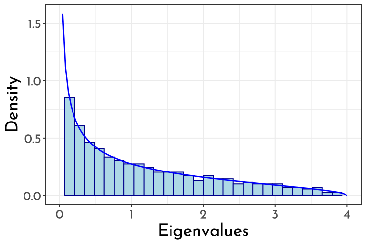
(a) Exponential(5)

(b) TN(0,1;0,10)

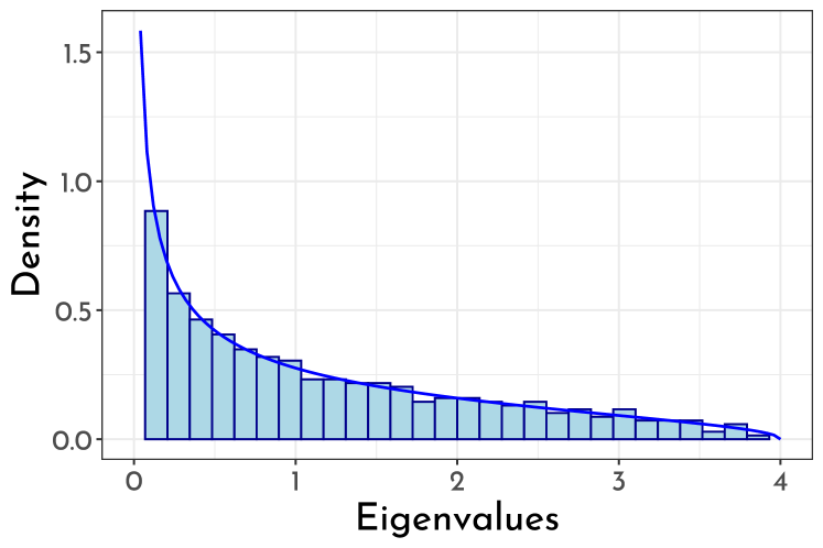
(c) Poisson(10)

Figure 1: Histograms of sample eigenvalues of $\boldsymbol{B}_{p,N}$ with $(p,n)=(500,500)$. The curves are density functions of their corresponding limiting spectral distribution.

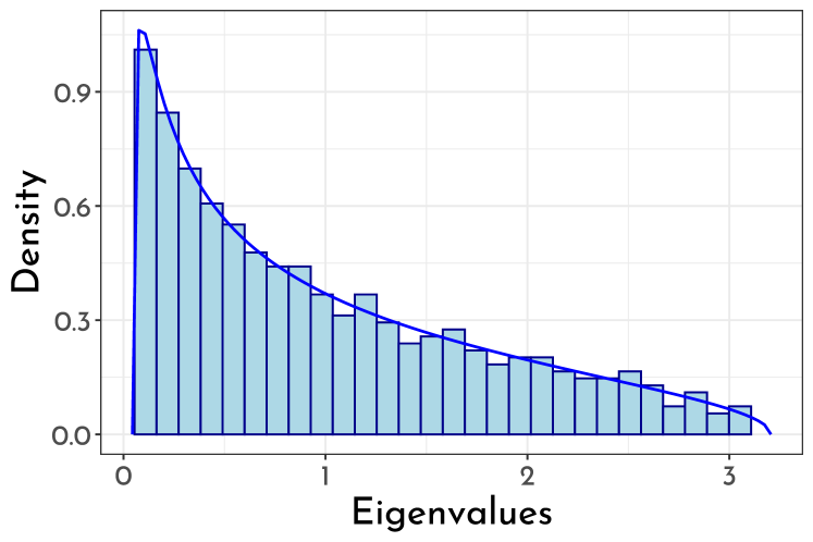
(a) Exponential(5)

(b) TN(0,1;0,10)

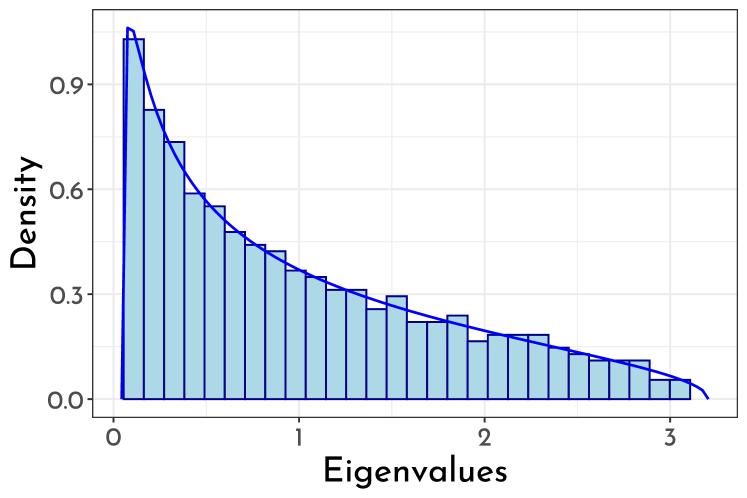
(c) Poisson(10)

Figure 2: Histograms of sample eigenvalues of $\boldsymbol{B}_{p,N}$ with $(p,n)=(500,800)$. The curves are density functions of their corresponding limiting spectral distribution.

3.2 CLT for LSS

In this section, we implement some simulation studies to examine finite-sample properties of some LSS for $\boldsymbol{B}_{p,N}$ by comparing their empirical means and variances with theoretical limiting values, as stated in Corollary 2.6.

In the following, we present the numerical simulation of CLT for LSS. First, we compare the empirical mean and variance of $G_{p,N}(x^{r})=\mathrm{tr}(\boldsymbol{B}_{p,N}^{r})-p\int x^{r}\mathop{}\!\mathrm{d}F^{c_{N}}(x)$, $r=1,2,3$, with their corresponding theoretical limits in Corollary 2.6. Two types of data distribution of $w_{ij}$ are consider:

1. $w_{ij}$ follows the exponential distribution with rate parameter $5$;

2. $w_{ij}$ follows the Chi-squared distribution with degree of freedom $1$.

Empirical mean and variance of $\{G_{p,N}(x^{r})\}$, $r=1,2,3$, are calculated for various combinations of $(p,n)$ with $p/n=3/4$ or $p/n=1$. For each pair of $(p,n)$, $2000$ independent replications are used to obtain the empirical values. Tables 1 – 2 report the empirical results for $\mathrm{Exp}(5)$ population and $\chi^{2}(1)$ population, respectively. As shown in Tables 1 – 2, the empirical mean and variance of $\{G_{p,N}(x^{r})\}$ closely match their respective theoretical limits under all scenarios. To verify the asymptotic normality of LSS, we draw the histogram of normalized LSS, $\overline{G}_{p,N}(x^{r})=(G_{p,N}(x^{r})-\mu_{r})/\sqrt{V_{r}}$, $r=1,2,3$, where $\mu_{r}$ and $V_{r}$ are defined in Corollary 2.6, and compare them with the standard normal density. Figures 3 and 4 depict the histograms of $\overline{G}_{p,N}(x^{r})$ for $\mathrm{Exp}(5)$ population with $p/n=1$ and $\chi^{2}(1)$ population with $p/n=3/4$, respectively. The histograms for the cases of $\mathrm{Exp}(5)$ population with $p/n=3/4$ and $\chi^{2}(1)$ population with $p/n=1$ exhibit similar patterns and are omitted for brevity. It can be seen from Figures 3 – 4 that all the histograms conform to the standard normal density, which fully supports our theoretical results.

Table 1: Empirical mean and variance of $G_{p,N}(x^{r})$, $r=1,2,3$, with $w_{ij}\sim\mathrm{Exp}(5)$.

			$G_{p,N}(x)$			$G_{p,N}(x^{2})$			$G_{p,N}(x^{3})$
	$p/n$	$n$	mean	var		mean	var		mean	var
Emp	$3/4$	100	-2.01	2.63		-4	36.54		-7.82	463.32
		200	-1.99	2.93		-3.85	39.73		-7.23	485.05
		300	-1.93	3.03		-3.57	40.3		-6.32	483.76
		400	-2.04	2.95		-3.98	38.78		-7.67	460.01
Theo			-2	3		-3.75	39		-6.81	457
Emp	$1$	100	-1.91	3.61		-3.83	64.09		-6.56	1064.75
		200	-1.96	3.89		-3.96	68.37		-6.91	1090.14
		300	-2.01	3.97		-4.06	68.7		-7.16	1082.72
		400	-1.98	3.71		-3.99	64.22		-7.07	1010.09
Theo			-2	4		-4	68		-7	1050

Table 2: Empirical mean and variance of $G_{p,N}(x^{r})$, $r=1,2,3$, with $w_{ij}\sim\chi^{2}(1)$.

			$G_{p,N}(x)$			$G_{p,N}(x^{2})$			$G_{p,N}(x^{3})$
	$p/n$	$n$	mean	var		mean	var		mean	var
Emp	$3/4$	100	-5.79	15.53		-24.19	888.99		-97.31	46790.03
		200	-5.96	16.74		-24.39	920.63		-96.17	45375.75
		300	-5.94	16.6		-23.75	882.92		-90.59	42487.68
		400	-5.88	17.51		-22.68	912.28		-81.2	42922.06
Theo			-6	18		-23	918		-83	41806.12
Emp	$1$	100	-5.92	20.81		-26.15	1563.02		-102.73	107846.2
		200	-5.98	23.01		-25.15	1639.95		-90.25	105467.9
		300	-5.81	21.82		-23.16	1526.34		-74.54	96864.11
		400	-6.13	23.18		-25.41	1599.96		-90.31	99475.82
Theo			-6	24		-24	1600		-80	96000

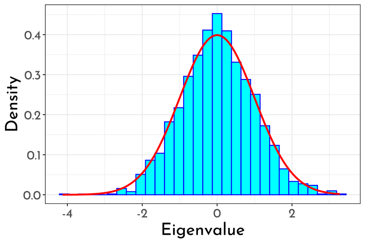
(a) $\overline{G}_{p,N}(x)$

(b) $\overline{G}_{p,N}(x^{2})$

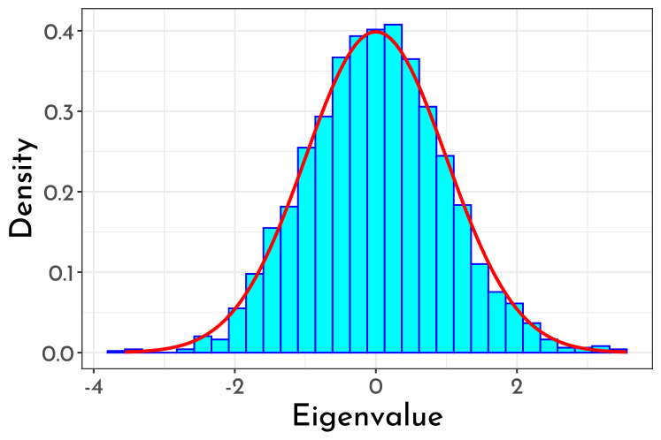
(c) $\overline{G}_{p,N}(x^{3})$

Figure 3: Histograms of normalized LSS $\overline{G}_{p,N}(x^{r})=(G_{p,N}(x^{r})-\mu_{r})/\sqrt{V_{r}}$, $r=1,2,3$, with $w_{ij}\sim\mathrm{Exp}(5)$ and $p=n=400$. The curves are density functions of the standard normal distribution.

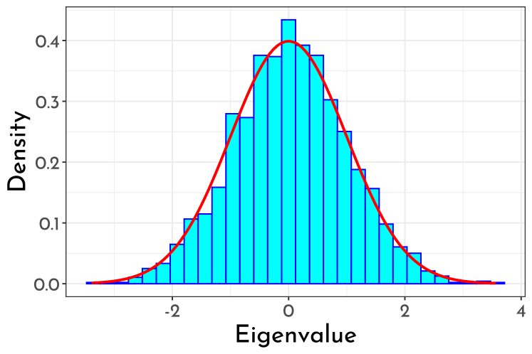
(a) $\overline{G}_{p,N}(x)$

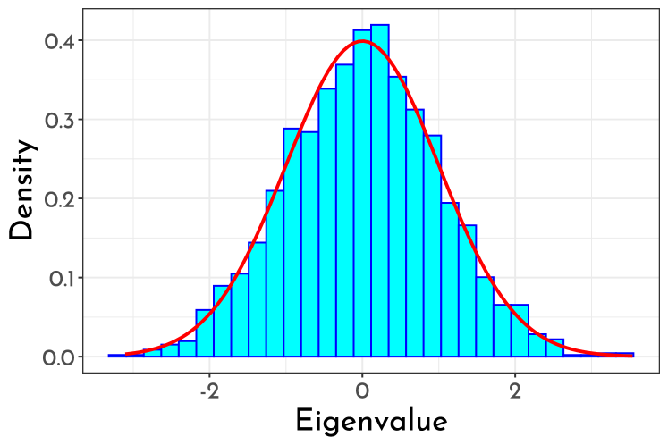
(b) $\overline{G}_{p,N}(x^{2})$

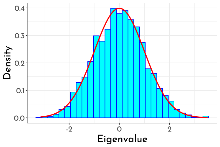
(c) $\overline{G}_{p,N}(x^{3})$

Figure 4: Histograms of normalized LSS $\overline{G}_{p,N}(x^{r})=(G_{p,N}(x^{r})-\mu_{r})/\sqrt{V_{r}}$, $r=1,2,3$, with $w_{ij}\sim\chi^{2}(1)$ and $p=300,n=400$. The curves are density functions of the standard normal distribution.

4 Proof of Theorem 2.5

In this section, we first present the difference between the CLT for centralized sample covariance $\boldsymbol{B}_{p}^{0}$ and unbiased sample covariance $\boldsymbol{B}_{p,N}$ by substitution principle in Section 4.1, where

$$\boldsymbol{B}_{p}^{0}=p^{2}\boldsymbol{S}_{n}^{0}=\frac{p^{2}}{n}(\boldsymbol{X}_{n}-\mathbb{E}\boldsymbol{X}_{n})^{\prime}(\boldsymbol{X}_{n}-\mathbb{E}\boldsymbol{X}_{n})=\frac{1}{n}\boldsymbol{Y}_{n}^{\prime}\boldsymbol{Y}_{n},\ \ \boldsymbol{B}_{p,N}=p^{2}\boldsymbol{S}_{n,N}=\frac{1}{N}(p\boldsymbol{X}_{n})^{\prime}\boldsymbol{C}_{n}(p\boldsymbol{X}_{n}),$$ (11)

and $\boldsymbol{Y}_{n}=(y_{ij})_{n\times p}$, $y_{ij}=\frac{w_{ij}}{\overline{w}_{i}}-1$ and $\overline{w}_{i}=\frac{1}{p}\sum_{j=1}^{p}w_{ij}$. By substituting the adjusted sample size $N=n-1$ for the actual sample size $n$ in the centering term, the unbiased sample covariance matrix $\boldsymbol{B}_{p,N}$ and the centralized sample covariance $\boldsymbol{B}_{p}^{0}$ share the same CLT (see, Section 4.1). The general strategy of the main proof of Theorem 2.5 is explained in the following and four major steps of the general strategy are presented in Section 4.3.

The general strategy of the proof follows the method established in Bai and Silverstein (2004) and Gao et al. (2017), with necessary adjustments for handling the sample covariance matrix of HCD, where conventional tools are not directly applicable. Our novel techniques play a pivotal role in overcoming these challenges. To begin with, we follow the strategy in Jiang (2004) to establish the LSD of $\boldsymbol{B}_{p,N}$ in Theorem 2.3. Then, we develop Proposition 2.4 to find the extreme eigenvalues of $\boldsymbol{B}_{p,N}$. Notably, these extreme eigenvalues are highly concentrated around two edges of the support, a crucial aspect for applying the Cauchy integral formula (12) and proving tightness. Given that compositional data $x_{ij}=w_{ij}/\sum_{j=1}^{p}w_{ij}$ are not i.i.d., dealing with the CLT for LSS of the unbiased sample covariance matrix $\boldsymbol{B}_{p,N}$ presents challenges. To address this, we employ the substitution principle (Zheng, Bai and Yao, 2015) to reduce the problem to the CLT for LSS of the centralized sample covariance $\boldsymbol{B}_{p}^{0}$. By substituting the adjusted sample size $N=n-1$ for the actual sample size $n$ in the centering term, both the unbiased sample covariance matrix $\boldsymbol{B}_{p,N}$ and the centralized sample covariance $\boldsymbol{B}_{p}^{0}$ share the same CLT (see Section 4.1). We then leverage the independence of samples to further study the CLT for LSS of $\boldsymbol{B}_{p}^{0}$. Specifically, we exploit the independence of samples to establish independence for $\boldsymbol{r}_{i}=\frac{1}{\sqrt{n}}\bigl{(}\frac{w_{i1}}{\overline{w}_{i}}-1,\ldots,\frac{w_{ip}}{\overline{w}_{i}}-1\bigr{)}^{\prime},i=1,2,\ldots,n$, and express $\boldsymbol{B}_{p}^{0}$ as $\boldsymbol{B}_{p}^{0}=\frac{1}{n}\boldsymbol{Y}_{n}^{\prime}\boldsymbol{Y}_{n}=\sum_{i=1}^{n}\boldsymbol{r}_{i}\boldsymbol{r}_{i}^{\prime}$. The ultimate goal is to establish the CLT for LSS of $\boldsymbol{B}_{p}^{0}$.

By the Cauchy integral formula, we have

$$\int f(x)\mathop{}\!\mathrm{d}G(x)=-\frac{1}{2\pi i}\oint_{\mathcal{C}}f(z)m_{G}(z)\mathop{}\!\mathrm{d}z$$ (12)

valid for any c.d.f $G$ and any analytic function $f$ on an open set containing the support of $G$, where $\oint_{\mathcal{C}}$ is the contour integration in the anti-clockwise direction. In our case, $G(x)=p(F^{\boldsymbol{B}_{p}^{0}}(x)-F^{c_{n}}(x))$. Therefore, the problem of finding the limiting distribution reduces to the study of $M_{p}(z)$ defined as follows:

$$M_{p}(z) =p\big{[}m_{p}(z)-m_{p}^{0}(z)\big{]}=n\big{[}\underline{m}_{p}(z)-\underline{m}_{p}^{0}(z)\big{]},$$

$$m_{p}(z) =m_{F^{\boldsymbol{B}_{p}^{0}}}(z)=\frac{1}{p}\mathrm{tr}\left[(\boldsymbol{B}_{p}^{0}-z\boldsymbol{I}_{p})^{-1}\right],\qquad m_{p}^{0}(z)=m_{F^{c_{n}}}(z),$$

$$\underline{m}_{p}(z) =m_{F^{\underline{\boldsymbol{B}}_{p}^{0}}}(z)=\frac{1}{p}\mathrm{tr}\left[(\underline{\boldsymbol{B}}_{p}^{0}-zI_{n})^{-1}\right],\qquad\underline{m}_{p}^{0}(z)=\underline{m}_{F^{c_{n}}}(z),$$

$$\underline{\boldsymbol{B}}_{p}^{0} =p^{2}\underline{\boldsymbol{S}}_{n}^{0}=\frac{p^{2}}{n}(\boldsymbol{X}_{n}-\mathbb{E}\boldsymbol{X}_{n})(\boldsymbol{X}_{n}-\mathbb{E}\boldsymbol{X}_{n})^{\prime}.$$

Note that the support of $F^{\boldsymbol{B}_{p,N}}$ is random. Fortunately, we have shown that the extreme eigenvalues of $\boldsymbol{B}_{p,N}$ are highly concentrated around two edges of the support of the limiting MP law $F^{c}(x)$ (see, Theorem 2.3, Proposition 2.4). Then the contour $\mathcal{C}$ can be appropriately chosen. Moreover, as in Bai and Silverstein (2004), by Proposition 2.4, we can replace the process $\{M_{p}(z),z\in\mathcal{C}\}$ by a slightly modified process $\{\widehat{M}_{p}(z),z\in\mathcal{C}\}$. Below we present the definitions of the contour $\mathcal{C}$ and the modified process $\widehat{M}_{p}(z)$. Let $x_{r}$ be any number greater than $\frac{\sigma^{2}}{\mu^{2}}(1+\sqrt{c})^{2}$. Let $x_{l}$ be any negative number if the left endpoint of (8) is zero. Otherwise we choose $x_{l}\in(0,\frac{\sigma^{2}}{\mu^{2}}(1-\sqrt{c})^{2})$. Now let $\mathcal{C}_{u}=\{x+iv_{0}:x\in[x_{l},x_{r}]\}$. Then we define $\mathcal{C}^{+}:=\{x_{l}+iv:v\in[0,v_{0}]\}\cup\mathcal{C}_{u}\cup\{x_{r}+iv:v\in[0,v_{0}]\}$, and $\mathcal{C}=\mathcal{C}^{+}\cup\overline{\mathcal{C}^{+}}$. Now we define the subsets $\mathcal{C}_{n}$ of $\mathcal{C}$ on which $M_{p}(\cdot)$ equals to $\widehat{M}_{p}(\cdot)$. Choose sequence $\{\varepsilon_{n}\}$ decreasing to zero satisfying for some $\alpha\in(0,1)$, $\varepsilon_{n}\geq n^{-\alpha}$. Let

$$\mathcal{C}_{l}=\left\{\begin{array}[]{ccc}\{x_{l}+iv:v\in[n^{-1}\varepsilon_{n},v_{0}]\}~{}~{}~{}~{}\mathrm{if}~{}x_{l}>0,\\ \{x_{l}+iv:v\in[0,v_{0}]\}~{}~{}~{}~{}~{}~{}~{}~{}~{}~{}\mathrm{if}~{}x_{l}<0,\end{array}\right.$$

and $\mathcal{C}_{r}=\{x_{r}+iv:v\in[n^{-1}\varepsilon,v_{0}]\}$. Then $\mathcal{C}_{n}=\mathcal{C}_{l}\cup\mathcal{C}_{u}\cup\mathcal{C}_{r}$. For $z=x+iv$, we define

$$\widehat{M}_{p}(z)=\begin{cases}M_{p}(z),&\text{ for }z\in\mathcal{C}_{n}\\ M_{p}(x_{r}+in^{-1}\varepsilon_{n}),&\text{ for }x=x_{r},v\in[0,n^{-1}\varepsilon_{n}],\text{ and if }x_{l}>0\\ M_{p}(x_{l}+in^{-1}\varepsilon_{n}),&\text{ for }x=x_{l},v\in[0,n^{-1}\varepsilon_{n}],\end{cases}$$

Most of the paper will deal with proving the following proposition.

Proposition 4.1.

Under Assumption 2.1 and 2.2, then $\widehat{M}_{p}(\cdot)$ converges weakly to a two-dimensional Gaussian process $M(\cdot)$ for $z\in\mathcal{C}$, with means

$$\mathbb{E}M(z)= -\underline{m}(z)\left[1-c\frac{\sigma^{4}}{\mu^{4}}\underline{m}^{2}(z)\Bigl{(}1+\frac{\sigma^{2}}{\mu^{2}}\underline{m}(z)\Bigr{)}^{-2}\right]^{-1}$$

$$\times\biggl{[}-z\underline{m}(z)\left(1+\frac{\sigma^{2}}{\mu^{2}}\underline{m}(z)\right)^{-1}\times\left(h_{1}m(z)+\frac{\sigma^{2}}{\mu^{2}}m(z)+\frac{\sigma^{2}}{\mu^{2}}\frac{1}{z}\right)$$

$$\qquad-cz^{2}\underline{m}^{2}(z)\left(1+\frac{\sigma^{2}}{\mu^{2}}\underline{m}(z)\right)^{-1}\left(\alpha_{1}m^{2}(z)+\alpha_{2}m^{2}(z)+2\frac{\sigma^{4}}{\mu^{4}}m^{\prime}(z)\right)$$

$$\qquad+c\frac{\sigma^{4}}{\mu^{4}}\underline{m}^{2}(z)\left(1+\frac{\sigma^{2}}{\mu^{2}}\underline{m}(z)\right)^{-3}\left(1-c\frac{\sigma^{4}}{\mu^{4}}\underline{m}^{2}(z)\left(1+\frac{\sigma^{2}}{\mu^{2}}\underline{m}(z)\right)^{-2}\right)^{-1}\biggr{]},$$ (13)

and covariance function

$$\mathrm{Cov}(M(z_{1}),M(z_{2})) =2\left[\frac{\underline{m}^{\prime}(z_{1})\underline{m}^{\prime}(z_{2})}{(\underline{m}(z_{1})-\underline{m}(z_{2}))^{2}}-\frac{1}{(z_{1}-z_{2})^{2}}\right]$$

$$\quad+c\left(\alpha_{1}+\alpha_{2}\right)\times\frac{\underline{m}^{\prime}(z_{1})\underline{m}^{\prime}(z_{2})}{(1+\sigma^{2}/\mu^{2}\underline{m}(z_{1}))^{2}(1+\sigma^{2}/\mu^{2}\underline{m}(z_{2}))^{2}}.$$ (14)

Now we explain how Theorem 2.5 follows from the above proposition. As in Bai and Silverstein (2004), with probability 1, $\left|\int f(z)(M_{p}(z)-\widehat{M}_{p}(z))\mathop{}\!\mathrm{d}z\right|\to 0$ as $n\to\infty$. Combining this observation with equation (12), Theorem 2.5 follows from Proposition 4.1. To prove Proposition 4.1, we decompose $M_{p}(z)$ into a random part $M^{(1)}_{p}(z)$ and a deterministic part $M^{(2)}_{p}(z)$ for $z\in\mathcal{C}_{n}$, that is, $M_{p}(z)=M_{p}^{(1)}(z)+M_{p}^{(2)}(z)$, where

$$M_{p}^{(1)}(z)=p\big{[}m_{p}(z)-\mathbb{E}m_{p}(z)\big{]}\quad\text{and}\quad M_{p}^{(2)}(z)=p\big{[}\mathbb{E}m_{p}(z)-m_{p}^{0}(z)\big{]}.$$

The random part contributes to the covariance function and the deterministic part contributes to the mean function. By Theorem 8.1 in Billingsley (1968), the proof of Proposition 4.1 is then complete if we can verify the following four steps:
Step 1 Truncation.
Step 2 Finite-dimensional convergence of $M_{p}^{(1)}(z)$ in distribution on $\mathcal{C}_{n}$ to a centered multivariate Gaussian random vector with covariance function given by (4.1).
Step 3 Tightness of the $M_{p}^{(1)}(z)$ for $z\in\mathcal{C}_{n}$.
Step 4 Convergence of the non-random part $M_{p}^{(2)}(z)$ to (4.1) on $z\in\mathcal{C}_{n}$.

The proof of these steps is presented in the coming sections. Before that, we introduce the substitution principle and crucial lemmas in Sections 4.1 and 4.2 respectively. The former explains the reduction of problem of the CLT for LSS of $\boldsymbol{B}_{p,N}$ to that of $\boldsymbol{B}_{p}^{0}$, while the latter provides essential lemmas for these four steps in proving the CLT for LSS of $\boldsymbol{B}_{p}^{0}$.

4.1 Substitution principle

By the Cauchy integral formula, we have

$$G_{p,N}(f) =-\frac{1}{2\pi i}\oint_{\mathcal{C}}f(z)\left[\operatorname{tr}(\boldsymbol{B}_{p,N}-z\boldsymbol{I}_{p})^{-1}-pm_{N}^{0}(z)\right]\mathop{}\!\mathrm{d}z$$ (15)

valid for any function $f$ analytic on an open set containing the support of $G_{p,N}$, where

$$m_{N}^{0}(z) \equiv m_{F^{c_{N}}}(z)=\frac{1}{\sigma^{2}/\mu^{2}(1-c_{N}-c_{N}zm_{N}^{0})-z},$$ (16)

$$\underline{m}_{N}^{0}(z) \equiv\underline{m}_{F^{c_{N}}}(z)=-\frac{1-c_{N}}{z}+cm_{N}^{0}(z),$$ (17)

$$z =-\frac{1}{\underline{m}_{N}^{0}(z)}+c_{N}\frac{\sigma^{2}/\mu^{2}}{1+\sigma^{2}/\mu^{2}\underline{m}_{N}^{0}(z)}$$ (18)

with $c_{N}=\frac{p}{N}$. To obtain the asymptotic distribution of $G_{p,N}(f)$, it is necessary to find the asymptotic distribution of $\operatorname{tr}(\boldsymbol{B}_{p,N}-z\boldsymbol{I}_{p})^{-1}-pm_{N}^{0}(z)$. To achieve this, we derive the following Lemma 4.2 whose proof is postponed to Section LABEL:pfsubstiprintr of the supplementary document.

Lemma 4.2.

Under conditions and notations in Theorem 2.5, as $n\rightarrow\infty$,

$$\operatorname{tr}(\boldsymbol{B}_{p,N}-z\boldsymbol{I}_{p})^{-1}-pm_{N}^{0}(z)=\operatorname{tr}(\boldsymbol{B}_{p}^{0}-z\boldsymbol{I}_{p})^{-1}-pm_{n}^{0}(z)+o_{P}(1).$$ (19)

By Lemma 4.2, the asymptotic distribution of $G_{p,N}(f)$ is identical to that of $G_{p}^{0}(f)$, i.e.,

$$G_{p,N}(f) =\sum_{i=1}^{p}f(\lambda_{i}(\boldsymbol{B}_{p,N}))-p\int f(x)\mathop{}\!\mathrm{d}F^{c_{N}}(x)\Longrightarrow\mathcal{N}(m(f),v(f)),$$ (20)

$$G_{p}^{0}(f) =\sum_{i=1}^{p}f(\lambda_{i}(\boldsymbol{B}_{p}^{0}))-p\int f(x)\mathop{}\!\mathrm{d}F^{c_{n}}(x)\Longrightarrow\mathcal{N}(m(f),v(f)),$$ (21)

a Guassian distribution whose parameters $m(f)$ and $v(f)$ depend only on the LSD $F^{c}(x)$ and $f$, where

$$G_{p}^{0}(f) =-\frac{1}{2\pi i}\oint_{\mathcal{C}}f(z)\left[\operatorname{tr}(\boldsymbol{B}_{p}^{0}-z\boldsymbol{I}_{p})^{-1}-pm_{n}^{0}(z)\right]\mathop{}\!\mathrm{d}z$$ (22)

and $c_{n}=\frac{p}{n}$, $m_{n}^{0}(z)=m_{F^{c_{n}}}(z)$ (note that we denote $m_{n}^{0}(z)$ as $m_{p}^{0}(z)$ in other sections except this subsection).

4.2 Some important lemmas

Before delving into the proof of the CLT for LSS, it is crucial to introduce three pivotal lemmas, representing novel contributions to this paper, that unveil concentration phenomena. Lemma 4.3 is crafted to estimate essential parameters, facilitating the derivation of estimates of any order. Concerning $\nu_{2}$ and $\nu_{12}$, the terms $h_{1}/p$ and $h_{2}/p$ emerge as non-negligible due to the multiplication by $p$ in the CLT. To address these parameters, we establish that the probability of the event $B^{c}_{p}(\epsilon)$ decays polynomially to $0$ and leverage Taylor expansion on the event $B_{p}(\epsilon)=\{\omega:|\overline{w}_{i}-\mu|\leq\epsilon,\overline{w}_{i}=\sum_{j=1}^{p}w_{ij}/p\}$ to handle the issue of dependence. The proof of the CLT for LSS relies on two pivotal steps: the moment inequality for random quadratic forms and the precise estimation of the expectation of the product of two random quadratic forms. Lemma 4.4 establishes the former step, essential for converting them into the corresponding traces, while Lemma 4.5 establishes the latter step, enabling the application of CLT for martingale differences. Both Lemma 4.4 and Lemma 4.5 heavily hinge on the estimation of parameters $\nu_{2}$, $\nu_{4}$, and $\nu_{12}$ in Lemma 4.3. The proof of Lemmas 4.3 – 4.5 are postponed to Sections LABEL:prfestsqu – LABEL:prfquadform of the supplementary document.

Lemma 4.3.

Suppose that $\boldsymbol{w}=\left(w_{1},\ldots,w_{p}\right)^{\prime}$ has i.i.d. entries with $\mathbb{E}w_{1}=\mu$, $\mathbb{E}(w_{1}-\mu)^{2}=\sigma^{2}$, and $\mathbb{E}\left|w_{1}-\mu\right|^{4}<\infty$, let $\overline{w}=\frac{1}{p}\sum_{j=1}^{p}w_{j}$, then there exists a constant $K>0$, such that for any $0<\epsilon<1/2$ and $p>0$,

$$\nu_{2}:=\mathbb{E}\Bigl{(}\frac{w_{1}}{\overline{w}}-1\Bigr{)}^{2} =\mathbb{E}\Bigl{(}\frac{w_{1}}{\mu}-1\Bigr{)}^{2}+\frac{1}{p}h_{1}+o(p^{-1}),$$ (23)

$$\nu_{12}:=\mathbb{E}\Bigl{(}\frac{w_{1}}{\overline{w}}-1\Bigr{)}^{2}\Bigl{(}\frac{w_{2}}{\overline{w}}-1\Bigr{)}^{2} =\Bigl{[}\mathbb{E}\Bigl{(}\frac{w_{1}}{\mu}-1\Bigr{)}^{2}\Bigr{]}^{2}+\frac{1}{p}h_{2}+o(p^{-1}),$$ (24)

$$\nu_{4}:=\mathbb{E}\Bigl{(}\frac{w_{1}}{\overline{w}}-1\Bigr{)}^{4} =\mathbb{E}\Bigl{(}\frac{w_{1}}{\mu}-1\Bigr{)}^{4}+o(1),$$ (25)

where

$$h_{1}=-2\frac{\mathbb{E}w_{11}^{3}}{\mu^{3}}+3\Bigl{(}\frac{\sigma^{2}}{\mu^{2}}\Bigr{)}^{2}+5\frac{\sigma^{2}}{\mu^{2}}+2,\ \ h_{2}=-8\frac{\sigma^{2}}{\mu^{2}}\frac{\mathbb{E}w_{11}^{3}}{\mu^{3}}+10\Bigl{(}\frac{\sigma^{2}}{\mu^{2}}\Bigr{)}^{3}+22\Bigl{(}\frac{\sigma^{2}}{\mu^{2}}\Bigr{)}^{2}+8\frac{\sigma^{2}}{\mu^{2}}.$$ (26)

Lemma 4.4.

Suppose that $\boldsymbol{w}=\left(w_{1},\ldots,w_{p}\right)^{\prime}$ has i.i.d. entries with $\mathbb{E}w_{1}=\mu$, $\mathbb{E}(w_{1}-\mu)^{2}=\sigma^{2}$, for any $p\times p$ matrix $\boldsymbol{A}$ and $q\geq 2$, we have there is a positive constant $K_{q}$ depending on $q$ such that

$$\mathbb{E}\Bigl{|}\boldsymbol{r}^{\prime}\boldsymbol{A}\boldsymbol{r}-\frac{1}{n}\nu_{2}\mathrm{tr}\boldsymbol{A}\Bigr{|}^{q} \leq K_{q}\Bigl{[}n^{-q}\Bigl{(}\bigl{(}\mathbb{E}\left|w_{1}\right|^{4}\mathrm{tr}(\boldsymbol{A}\boldsymbol{A}^{\prime})\bigr{)}^{q/2}+\mathbb{E}|w_{1}|^{2q}\mathrm{tr}(\boldsymbol{A}\boldsymbol{A}^{\prime})^{q/2}\Bigr{)}$$

$$\qquad\qquad+n^{q}\mathbb{P}\bigl{(}B^{c}_{p}(\epsilon)\bigr{)}\|\boldsymbol{A}\|^{q}+n^{-q}\|\boldsymbol{A}^{q}\|h_{1}^{q}\Bigr{]},$$ (27)

where $\boldsymbol{r}=\frac{1}{\sqrt{n}}(w_{1}/\overline{w}-1,\dots,w_{p}/\overline{w}-1)^{\prime}$, $h_{1}$ is in (26), $B_{p}(\epsilon)=\{\omega:|\overline{w}-u|\leq\epsilon,\overline{w}=\sum_{j=1}^{p}w_{j}/p\},$ and

$$\mathbb{P}(B^{c}_{p}(\epsilon))\leq K\epsilon^{-kq_{1}}(\sigma^{kq_{1}}p^{-kq_{1}/2}+p^{-kq_{1}+1}\mathbb{E}\left|w_{1}\right|^{kq_{1}}),$$ (28)

in which $\epsilon,k,q_{1}>0$ are constants. Furthermore, if $\|\boldsymbol{A}\|\leq K$ and $|w_{j}-\mu|<\delta_{n}\sqrt{n}$ for all $j=1,\ldots,p$, then, for any $q\geq 2$,

$$\mathbb{E}\Bigl{|}\boldsymbol{r}^{\prime}\boldsymbol{A}\boldsymbol{r}-\frac{1}{n}\nu_{2}\mathrm{tr}\boldsymbol{A}\Bigr{|}^{q}\leq K_{q}n^{-1}\delta_{n}^{2q-4}.$$

Lemma 4.5.

Suppose that $\boldsymbol{w}=\left(w_{1},\ldots,w_{p}\right)^{\prime}$ has i.i.d. entries with $\mathbb{E}w_{1}=\mu$, $\mathbb{E}(w_{1}-\mu)^{2}=\sigma^{2}$, $\boldsymbol{A}$ and $\boldsymbol{B}$ are $p\times p$ matrices , if $\|\boldsymbol{A}\|\leq K$ and $\|\boldsymbol{B}\|\leq K$, then

$$\ \ \ \ \mathbb{E}\Bigl{(}\boldsymbol{r}^{\prime}A\boldsymbol{r}-\frac{1}{n}\nu_{2}\mathrm{tr}\boldsymbol{A}\Bigr{)}\Bigl{(}\boldsymbol{r}^{\prime}\boldsymbol{B}\boldsymbol{r}-\frac{1}{n}\nu_{2}\mathrm{tr}\boldsymbol{B}\Bigr{)}$$

$$=\frac{1}{n^{2}}(\nu_{4}-3\nu_{12})\sum_{i=1}^{p}A_{ii}B_{ii}+\frac{1}{n^{2}}\nu_{12}\bigl{(}\mathrm{tr}(\boldsymbol{A}\boldsymbol{B}^{\prime})+\mathrm{tr}(\boldsymbol{A}\boldsymbol{B})\bigr{)}+\frac{1}{n^{2}}(\nu_{12}-\nu_{2}^{2})\mathrm{tr}\boldsymbol{A}\mathrm{tr}\boldsymbol{B}+o(n^{-1}).$$

4.3 CLT for LSS of the centralized sample covariance $B_{p}^{0}$

Step 1: Truncation. We begin the proof of Proposition 4.1 with the replacement of the entries of $\boldsymbol{W}_{n}$ with truncated variables. We can choose a positive sequence of $\{\delta_{n}\}$ such that

$$\delta_{n}\rightarrow 0,\quad\delta_{n}n^{1/4}\rightarrow\infty,\quad\delta_{n}^{-4}\mathbb{E}w_{11}^{4}I_{\{|w_{11}-\mu|\geq\delta_{n}\sqrt{n}\}}\rightarrow 0.$$

Let $\hat{\boldsymbol{B}}_{p}^{0}=\frac{p^{2}}{n}(\hat{\boldsymbol{X}}_{n}-\mathbb{E}\hat{\boldsymbol{X}}_{n})^{\prime}(\hat{\boldsymbol{X}}_{n}-\mathbb{E}\hat{\boldsymbol{X}}_{n})$, where $\hat{\boldsymbol{W}}_{n}$ is $n\times p$ matrix having $\hat{w}_{ij}=w_{ij}I_{\{|w_{ij}-\mu|<\delta_{n}\sqrt{n}\}}$. We then have

$$\mathbb{P}(\boldsymbol{B}_{p}^{0}\neq\hat{\boldsymbol{B}}_{p}^{0}) \leq\mathbb{P}\Big{(}\bigcup_{i\leq n,j\leq p}(|w_{ij}-\mu|\geq\delta_{n}\sqrt{n})\Big{)}\leq np\cdot\mathbb{P}(|w_{ij}-\mu|\geq\delta_{n}\sqrt{n})$$

$$\leq K\delta_{n}^{-4}\int_{\{|w_{ij}-\mu|\geq\delta_{n}\sqrt{n}\}}|w_{11}|^{4}=o(1).$$

Let $\hat{G}_{p}^{0}(x)$ be $G_{p}^{0}(x)$ with $\boldsymbol{B}_{p}^{0}$ replaced by $\hat{\boldsymbol{B}}_{p}^{0}$, then $\mathbb{P}(\hat{G}_{p}^{0}(x)\neq G_{p}^{0}(x))\leq\mathbb{P}(\boldsymbol{B}_{p}^{0}\neq\hat{\boldsymbol{B}}_{p}^{0})=o(1)$. In view of the above, we obtain

$$\int f_{j}(x)\mathop{}\!\mathrm{d}G_{p}^{0}(x)=\int f_{j}(x)\mathop{}\!\mathrm{d}\hat{G}_{p}^{0}(x)+o_{P}(1).$$

To simplify notation, we below still use $w_{ij}$ instead of $\hat{w}_{ij}$, and assume that

$$|w_{ij}-\mu|<\delta_{n}\sqrt{n},\quad\mathbb{E}w_{ij}=\mu>0,\quad\mathbb{E}|w_{ij}-\mu|^{2}=\sigma^{2},\quad\mathbb{E}|w_{ij}-\mu|^{4}<\infty.$$ (29)

Step 2: Finite dimensional convergence of $M^{(1)}_{p}(z)$ in distribution

Lemma 4.6.

Under conditions and notations in Theorem 2.5, as $p\rightarrow\infty$, for any set of $r$ points $\{z_{1},z_{2},...,z_{r}\}\bigcup\mathcal{C}$, the random vector $\bigl{(}M_{p}^{(1)}(z_{1}),\ldots,M_{p}^{(1)}(z_{r})\bigr{)}$ converges weakly to a $r$-dimensional centered Gaussian distribution with covariance function in (4.1).

We now proceed to the proof of this lemma. By the fact that a random vector is multivariate normally distributed if and only if every linear combination of its components is normally distributed, we need only show that, for any positive integer $r$ and any complex sequence ${a_{j}}$, the sum

$$\sum_{j=1}^{r}a_{j}M^{(1)}_{p}(z_{j})$$

converges weakly to a Gaussian random variable. To this end, we first decompose the random part $M^{(1)}_{p}(z)$ as a sum of martingale difference, which is given in (37). Then, we apply the martingale CLT (Lemma LABEL:billin) to obtain the asymptotic distribution of $M^{(1)}_{p}(z)$. Details of these two steps are provided in the following two parts.

Part 1: Martingale difference decomposition of $M^{(1)}_{p}(z)$. First, we introduce some notations. In the following proof, we assume that $v=\Im z\geq v_{0}>0$. Moreover, for $j=1,2,\ldots,n$, let

$$\boldsymbol{r}_{j}=\frac{1}{\sqrt{n}}\left(\frac{w_{j1}}{\overline{w}_{j}}-1,\ldots,\frac{w_{jp}}{\overline{w}_{j}}-1\right)^{\prime},\;\boldsymbol{D}(z)=\boldsymbol{B}_{p}^{0}-z\boldsymbol{I}_{p},\;\boldsymbol{D}_{j}(z)=\boldsymbol{D}(z)-\boldsymbol{r}_{j}\boldsymbol{r}_{j}^{\prime},$$

$$\beta_{j}(z)=\frac{1}{1+\boldsymbol{r}_{j}^{\prime}\boldsymbol{D}_{j}^{-1}(z)\boldsymbol{r}_{j}},\ \ \overline{\beta}_{j}(z)=\frac{1}{1+\frac{1}{n}\nu_{2}\mathrm{tr}\boldsymbol{D}^{-1}_{j}(z)},\;b_{p}(z)=\frac{1}{1+\frac{1}{n}\nu_{2}\mathbb{E}\mathrm{tr}\boldsymbol{D}_{1}^{-1}(z)},$$

$\varepsilon_{j}(z)=\boldsymbol{r}_{j}^{\prime}\boldsymbol{D}_{j}^{-1}(z)\boldsymbol{r}_{j}-\frac{1}{n}\nu_{2}\mathrm{tr}\boldsymbol{D}_{j}^{-1}(z)$ and $\delta_{j}(z)=\boldsymbol{r}_{j}^{\prime}\boldsymbol{D}_{j}^{-2}(z)\boldsymbol{r}_{j}-\frac{1}{n}\nu_{2}\mathrm{tr}\boldsymbol{D}_{j}^{-2}(z)=\frac{d}{\mathop{}\!\mathrm{d}z}\varepsilon_{j}(z)$. By Lemma 4.4, we have, for any $r\geq 2$,

$$\mathbb{E}|\varepsilon_{j}(z)|^{r}\leq\frac{K}{v^{2r}}n^{-1}\delta_{n}^{2r-4}\ \ and\ \ \mathbb{E}|\delta_{j}(z)|^{r}\leq\frac{K}{v^{2r}}n^{-1}\delta_{n}^{2r-4}.$$ (30)

It is easy to see that

$$\boldsymbol{D}^{-1}(z)-\boldsymbol{D}_{j}^{-1}(z)=-\boldsymbol{D}_{j}^{-1}(z)\boldsymbol{r}_{j}\boldsymbol{r}_{j}^{\prime}\boldsymbol{D}_{j}^{-1}(z)\beta_{j}(z),$$ (31)

where we use the formula that $\boldsymbol{A}_{1}^{-1}-\boldsymbol{A}_{2}^{-1}=\boldsymbol{A}_{2}^{-1}(\boldsymbol{A}_{2}-\boldsymbol{A}_{1})\boldsymbol{A}_{1}^{-1}$ holds for any two invertible matrices $\boldsymbol{A}_{1}$ and $\boldsymbol{A}_{2}$. Note that $|\beta_{j}(z)|$, $|\overline{\beta}_{j}(z)|$ and $|b_{n}(z)|$ are bounded by $\frac{|z|}{v}$. We also get that for any $j$,

$$\mathbb{E}(\boldsymbol{r}_{j}\boldsymbol{r}_{j}^{\prime})=\frac{1}{n}\nu_{2}\left(-\frac{1}{p-1}\boldsymbol{1}_{p}\boldsymbol{1}^{\prime}_{p}+\frac{1}{p-1}\boldsymbol{I}_{p}+\boldsymbol{I}_{p}\right).$$ (32)

Let $\mathbb{E}_{0}(\cdot)$ denote expectation and $\mathbb{E}_{j}(\cdot)$ denote conditional expectation with respect to the $\sigma$-field generated by $\boldsymbol{r}_{1},\boldsymbol{r}_{2},\ldots,\boldsymbol{r}_{j}$, where $j=1,2,\ldots,n$. Next, we write $M_{p}^{(1)}(z)$ as a sum of martingale difference sequences (MDS), and then utilize the CLT of MDS (Lemma LABEL:billin) to derive the asymptotic distribution of $M_{p}^{(1)}(z)$, which can be written as

$$p[m_{p}(z)-\mathbb{E}M_{p}(z)]=\sum^{n}_{j=1}[\mathrm{tr}(\mathbb{E}_{j}-\mathbb{E}_{j-1})\boldsymbol{D}^{-1}(z)]=-\sum^{n}_{j=1}(\mathbb{E}_{j}-\mathbb{E}_{j-1})\beta_{j}(z)\boldsymbol{r}_{j}^{\prime}\boldsymbol{D}_{j}^{-2}(z)\boldsymbol{r}_{j}.$$ (33)

Write $\beta_{j}(z)=\overline{\beta}_{j}(z)-\beta_{j}(z)\overline{\beta}_{j}(z)\varepsilon_{j}(z)=\overline{\beta}_{j}(z)-\overline{\beta}_{j}^{2}(z)\varepsilon_{j}(z)+\overline{\beta}_{j}^{2}(z)\beta_{j}(z)\varepsilon_{j}^{2}(z)$. From this and the definition of $\delta_{j}(z)$, (33) has the following expression

$$(\mathbb{E}_{j}-\mathbb{E}_{j-1})\beta_{j}(z)\boldsymbol{r}_{j}^{\prime}\boldsymbol{D}_{j}^{-2}(z)\boldsymbol{r}_{j}=(\mathbb{E}_{j}-\mathbb{E}_{j-1})\big{[}\big{(}\overline{\beta}_{j}(z)-\overline{\beta}_{j}^{2}(z)\varepsilon_{j}(z)$$

$$\ \ \ \ \ \ \ \ \ \ \ \ \ \ \ +\overline{\beta}_{j}^{2}(z)\beta_{j}(z)\varepsilon_{j}^{2}(z)\big{)}\big{(}\delta_{j}(z)+\frac{1}{n}\nu_{2}\mathrm{tr}\boldsymbol{D}_{j}^{-2}(z)\big{)}\big{]}$$

$$= -Y_{j}(z)+\mathbb{E}_{j-1}Y_{j}(z)-(\mathbb{E}_{j}-\mathbb{E}_{j-1})\big{[}\overline{\beta}_{j}^{2}(z)\big{(}\varepsilon_{j}(z)\delta_{j}(z)-\beta_{j}(z)\boldsymbol{r}_{j}^{\prime}\boldsymbol{D}_{j}^{-2}(z)\boldsymbol{r}_{j}\varepsilon_{j}^{2}(z)\big{)}\big{]},$$ (34)

where the second equality uses the fact that $(\mathbb{E}_{j}-\mathbb{E}_{j-1})\overline{\beta}_{j}(z)\mathrm{tr}\boldsymbol{D}_{j}^{-2}(z)=0$, and

$$Y_{j}(z)=-\mathbb{E}_{j}\Big{(}\overline{\beta}_{j}(z)\delta_{j}(z)-\overline{\beta}_{j}^{2}(z)\varepsilon_{j}(z)\frac{1}{n}\nu_{2}\mathrm{tr}\boldsymbol{D}_{j}^{-2}(z)\Big{)}=-\mathbb{E}_{j}\frac{\mathop{}\!\mathrm{d}}{\mathop{}\!\mathrm{d}z}\big{(}\overline{\beta}_{j}(z)\varepsilon_{j}(z)\big{)}.$$

By (30), we have

$$\mathbb{E}\Big{|}\sum^{n}_{j=1}(\mathbb{E}_{j}-\mathbb{E}_{j-1})\overline{\beta}_{j}^{2}(z)\varepsilon_{j}(z)\delta_{j}(z)\Big{|}^{2} \leq 4\sum^{n}_{j=1}\mathbb{E}\big{|}\overline{\beta}_{j}^{2}(z)\varepsilon_{j}(z)\delta_{j}(z)\big{|}^{2}=o(1),$$ (35)

here we leverage the the martingale difference property of $(\mathbb{E}_{j}-\mathbb{E}_{j-1})\overline{\beta}_{j}^{2}(z)\varepsilon_{j}(z)\delta_{j}(z)$. Thus, $\sum^{n}_{j=1}(\mathbb{E}_{j}-\mathbb{E}_{j-1})\overline{\beta}_{j}^{2}(z)\varepsilon_{j}(z)\delta_{j}(z)$ converges to $0$ in probability. By the same argument, we have

$$\sum^{n}_{j=1}(\mathbb{E}_{j}-\mathbb{E}_{j-1})\overline{\beta}_{j}^{2}(z)\beta_{j}(z)\boldsymbol{r}_{j}^{\prime}\boldsymbol{D}_{j}^{-2}(z)\boldsymbol{r}_{j}\varepsilon_{j}^{2}(z)\stackrel{{\scriptstyle i.p.}}{{\rightarrow}}0.$$ (36)

Then, equations (33) – (36) imply that

$$M^{(1)}_{p}(z)=\sum_{j=1}^{n}\{Y_{j}(z)-\mathbb{E}_{j-1}Y_{j}(z)\}+o_{P}(1),$$ (37)

where $\left\{Y_{j}(z)-\mathbb{E}_{j-1}Y_{j}(z),j=1,\ldots,n\right\}$ is a sequence of martingale difference.

Part 2: Application of martingales CLT to (37). To prove finite-dimensional convergence of $M_{p}^{(1)}(z)$, $z\in\mathcal{C}$, we need only to consider the limit of the following martingale difference decomposition:

$$\sum_{i=1}^{r}\alpha_{i}M^{(1)}_{p}(z_{i})=\sum^{r}_{i=1}\alpha_{i}\sum^{n}_{j=1}(Y_{j}(z_{i})-\mathbb{E}_{j-1}Y_{j}(z_{i}))+o(1)=\sum^{n}_{j=1}\sum^{r}_{i=1}\alpha_{i}(Y_{j}(z_{i})-\mathbb{E}_{j-1}Y_{j}(z_{i}))+o(1),$$

where $\Im(z_{i})\neq 0$, $\{\alpha_{i}:i=1,2,\ldots,r\}$ are constants. We apply the martingale CLT (Lemma LABEL:billin) to this martingale difference decomposition of $\sum_{i=1}^{r}\alpha_{i}M^{(1)}_{p}(z_{i})$. To this end, we need to check two conditions:

Condition 4.7.

$$\qquad\sum^{n}_{j=1}\mathbb{E}\left(\left|\sum^{r}_{i=1}\alpha_{i}\left(Y_{j}(z_{i})-\mathbb{E}_{j-1}Y_{j}(z_{i})\right)\right|^{2}I_{\{|\sum^{r}_{i=1}\alpha_{i}\left(Y_{j}(z_{i})+\mathbb{E}_{j-1}Y_{j}(z_{i})\right)|\geq\varepsilon\}}\right)\rightarrow 0.$$ (38)

Condition 4.8.

$$\sum^{n}_{j=1}\mathbb{E}_{j-1}\bigl{[}\bigl{(}Y_{j}(z_{1})-\mathbb{E}_{j-1}Y_{j}(z_{1})\bigr{)}\bigl{(}Y_{j}(z_{2})-\mathbb{E}_{j-1}Y_{j}(z_{2})\bigr{)}\bigr{]}$$ (39)

converges in probability to a constant.

First, we verify Condition 4.7. By Lemma 4.4, we obtain

$$\mathbb{E}|Y_{j}(z)|^{4}\leq K\mathbb{E}|\varepsilon_{j}(z)|^{4}=o\left(\frac{1}{p}\right).$$ (40)

Furthermore, by Jensen’s inequality and (40),

$$\mathbb{E}|\mathbb{E}_{j-1}Y_{j}(z)|^{4}\leq\mathbb{E}(\mathbb{E}_{j-1}|Y_{j}(z)|^{4})=\mathbb{E}|Y_{j}(z)|^{4}=o\left(\frac{1}{p}\right).$$ (41)

It follows from (40) and (41) that

$$\text{the left hand side of}\ \ \eqref{condi1eq}\leq \;K\left(\frac{1}{\varepsilon^{2}}\sum^{n}_{j=1}\mathbb{E}\left|\sum^{r}_{i=1}\alpha_{i}Y_{j}(z_{i})\right|^{4}+\frac{1}{\varepsilon^{2}}\sum^{n}_{j=1}\mathbb{E}\left|\sum^{r}_{i=1}\alpha_{i}\mathbb{E}_{j-1}Y_{j}(z_{i})\right|^{4}\right)\rightarrow 0.$$

Then, we verify Condition 4.8. Since

$$\eqref{condi2eq} =\sum^{n}_{j=1}\mathbb{E}_{j-1}[Y_{j}(z_{1})Y_{j}(z_{2})]-\sum^{n}_{j=1}[\mathbb{E}_{j-1}Y_{j}(z_{1})][\mathbb{E}_{j-1}Y_{j}(z_{2})]$$

$$=\frac{\partial^{2}}{\partial z_{1}\partial z_{2}}\Big{(}\sum^{n}_{j=1}\mathbb{E}_{j-1}\big{[}\mathbb{E}_{j}\big{(}\overline{\beta}_{j}(z_{1})\varepsilon_{j}(z_{1})\big{)}\mathbb{E}_{j}\big{(}\overline{\beta}_{j}(z_{2})\varepsilon_{j}(z_{2})\big{)}\big{]}\Big{)}$$

$$\ \ \ \ -\frac{\partial^{2}}{\partial z_{1}\partial z_{2}}\Big{(}\sum^{n}_{j=1}\big{[}\mathbb{E}_{j-1}\overline{\beta}_{j}(z_{1})\varepsilon_{j}(z_{1})][\mathbb{E}_{j-1}\overline{\beta}_{j}(z_{2})\varepsilon_{j}(z_{2})\big{]}\Big{)},$$

it is enough to consider the limits of

$$\sum^{n}_{j=1}\mathbb{E}_{j-1}\big{[}\mathbb{E}_{j}\big{(}\overline{\beta}_{j}(z_{1})\varepsilon_{j}(z_{1})\big{)}\mathbb{E}_{j}\big{(}\overline{\beta}_{j}(z_{2})\varepsilon_{j}(z_{2})\big{)}\big{]}$$ (42)

and

$$\sum^{n}_{j=1}\big{[}\mathbb{E}_{j-1}\overline{\beta}_{j}(z_{1})\varepsilon_{j}(z_{1})][\mathbb{E}_{j-1}\overline{\beta}_{j}(z_{2})\varepsilon_{j}(z_{2})\big{]}.$$ (43)

The limit of (43) is provided in the following lemma.

Lemma 4.9.

Under conditions and notations in Theorem 2.5, then

$$\sum^{n}_{j=1}\big{[}\mathbb{E}_{j-1}\overline{\beta}_{j}(z_{1})\varepsilon_{j}(z_{1})][\mathbb{E}_{j-1}\overline{\beta}_{j}(z_{2})\varepsilon_{j}(z_{2})\big{]}\stackrel{{\scriptstyle i.p.}}{{\rightarrow}}0.$$

The proof of Lemma 4.9 is postponed to Section LABEL:prfej-1term0 of the supplementary document. By Lemma 4.9, the remaining work is to consider the limit of (42). Since the following inequalities hold:

$$\big{|}\mathrm{tr}\big{(}\boldsymbol{D}^{-1}(z)-\boldsymbol{D}_{j}^{-1}(z)\big{)}\boldsymbol{A}\big{|} \leq\frac{\|\boldsymbol{A}\|}{\Im(z)},$$ (44)

$$\mathbb{E}\big{|}\frac{1}{n}\nu_{2}\mathrm{tr}\boldsymbol{D}^{-1}(z)-\mathbb{E}\frac{1}{n}\nu_{2}\mathrm{tr}\boldsymbol{D}^{-1}(z)\big{|}^{q} \leq C_{q}n^{-q/2}v_{0}^{-q},$$ (45)

$$\mathbb{E}\big{|}\overline{\beta}_{j}(z_{i})-b_{n}(z_{i})\big{|}^{2} \leq\frac{K|z_{i}|^{4}}{nv_{0}^{6}},$$ (46)

it is enough to prove that

$$b_{p}(z_{1})b_{p}(z_{2})\sum^{n}_{j=1}\mathbb{E}_{j-1}\big{[}\mathbb{E}_{j}\big{(}\varepsilon_{j}(z_{1})\big{)}\mathbb{E}_{j}\big{(}\varepsilon_{j}(z_{2})\big{)}\big{]}$$ (47)

converges to a constant in probability, which further gives the limit of (42). By Lemma 4.5, we have

$$\eqref{bprecltlim} =b_{p}(z_{1})b_{p}(z_{2})\sum_{j=1}^{n}\biggl{[}\sum_{i=1}^{p}\frac{1}{n^{2}}(\nu_{4}-3\nu_{12})\mathbb{E}_{j}(\boldsymbol{D}_{j}^{-1}(z_{1}))_{ii}\mathbb{E}_{j}(\boldsymbol{D}_{j}^{-1}(z_{2}))_{ii}$$

$$+\frac{1}{n^{2}}\nu_{12}\Bigl{(}\mathrm{tr}\left[\mathbb{E}_{j}\boldsymbol{D}_{j}^{-1}(z_{1})\mathbb{E}_{j}(\boldsymbol{D}_{j}^{-1}(z_{2}))^{\prime}\right]+\mathrm{tr}\left[\mathbb{E}_{j}\boldsymbol{D}_{j}^{-1}(z_{1})\mathbb{E}_{j}\boldsymbol{D}_{j}^{-1}(z_{2})\right]\Bigr{)}$$

$$+\frac{1}{n^{2}}(\nu_{12}-\nu_{2}^{2})\mathrm{tr}\left[\mathbb{E}_{j}\boldsymbol{D}_{j}^{-1}(z_{1})\right]\mathrm{tr}\left[\mathbb{E}_{j}\boldsymbol{D}_{j}^{-1}(z_{2})\right]\biggr{]}+o(1)=:I_{1}+I_{2}+I_{3}+I_{4}+o(1),$$ (48)

where

$$I_{1} =\frac{1}{n^{2}}(\nu_{4}-3\nu_{12})b_{p}(z_{1})b_{p}(z_{2})\sum_{j=1}^{n}\sum_{i=1}^{p}\mathbb{E}_{j}(\boldsymbol{D}_{j}^{-1}(z_{1}))_{ii}\mathbb{E}_{j}(\boldsymbol{D}_{j}^{-1}(z_{2}))_{ii},$$

$$I_{2} =\frac{1}{n^{2}}\nu_{12}b_{p}(z_{1})b_{p}(z_{2})\sum_{j=1}^{n}\mathrm{tr}\left[\mathbb{E}_{j}\boldsymbol{D}_{j}^{-1}(z_{1})\mathbb{E}_{j}(\boldsymbol{D}_{j}^{-1}(z_{2}))^{\prime}\right],$$

$$I_{3} =\frac{1}{n^{2}}\nu_{12}b_{p}(z_{1})b_{p}(z_{2})\sum_{j=1}^{n}\mathrm{tr}\left[\mathbb{E}_{j}\boldsymbol{D}_{j}^{-1}(z_{1})\mathbb{E}_{j}\boldsymbol{D}_{j}^{-1}(z_{2})\right],$$

$$I_{4} =\frac{1}{n^{2}}(\nu_{12}-\nu_{2}^{2})b_{p}(z_{1})b_{p}(z_{2})\sum_{j=1}^{n}\mathrm{tr}\left[\mathbb{E}_{j}\boldsymbol{D}_{j}^{-1}(z_{1})\right]\mathrm{tr}\left[\mathbb{E}_{j}\boldsymbol{D}_{j}^{-1}(z_{2})\right].$$

In the following Steps (i)-(iii), we derive as $p\to\infty$,

$$\frac{\partial^{2}}{\partial z_{1}\partial z_{2}}I_{1}\stackrel{{\scriptstyle i.p.}}{{\rightarrow}}c\alpha_{1}\frac{\underline{m}^{\prime}(z)\underline{m}^{\prime}(z_{2})}{\big{(}1+\frac{\sigma^{2}}{\mu^{2}}\underline{m}(z_{1})\big{)}^{2}\big{(}1+\frac{\sigma^{2}}{\mu^{2}}\underline{m}(z_{2})\big{)}^{2}},$$ (49)

$$\frac{\partial^{2}}{\partial z_{1}\partial z_{2}}I_{2},\ \frac{\partial^{2}}{\partial z_{1}\partial z_{2}}I_{3}\stackrel{{\scriptstyle i.p.}}{{\rightarrow}}\frac{\partial}{\partial z_{2}}\big{(}\frac{\partial a(z_{1},z_{2})/\partial z_{1}}{1-a(z_{1},z_{2})}\big{)}=\frac{\underline{m}^{\prime}(z_{1})\underline{m}^{\prime}(z_{2})}{(\underline{m}(z_{1})-\underline{m}(z_{2}))^{2}}-\frac{1}{(z_{1}-z_{2})^{2}},$$ (50)

$$\frac{\partial^{2}}{\partial z_{1}\partial z_{2}}I_{4}\stackrel{{\scriptstyle i.p.}}{{\rightarrow}}c\Bigl{(}h_{2}-2\frac{\sigma^{2}}{\mu^{2}}h_{1}\Bigr{)}\frac{\underline{m}^{\prime}(z_{1})\underline{m}^{\prime}(z_{2})}{\big{(}1+\frac{\sigma^{2}}{\mu^{2}}\underline{m}(z_{1})\big{)}^{2}\big{(}1+\frac{\sigma^{2}}{\mu^{2}}\underline{m}(z_{2})\big{)}^{2}}.$$ (51)

Step (i): Consider $I_{2}$ and $I_{3}$. Let $\boldsymbol{D}_{ij}(z)=\boldsymbol{D}(z)-\boldsymbol{r}_{i}\boldsymbol{r}_{i}^{\prime}-\boldsymbol{r}_{j}\boldsymbol{r}_{j}^{\prime}$, $b_{1}(z)=\frac{1}{1+\frac{1}{n}\nu_{2}\mathbb{E}\mathrm{tr}\boldsymbol{D}_{12}^{-1}(z)}$ and $\beta_{ij}(z)=\frac{1}{1+\boldsymbol{r}_{i}^{\prime}\boldsymbol{D}_{ij}^{-1}(z)\boldsymbol{r}_{i}}$. We have the equality $\boldsymbol{D}_{j}(z_{1})+z_{1}\boldsymbol{I}_{p}-\frac{n-1}{n}\nu_{2}b_{1}(z_{1})\boldsymbol{I}_{p}=\sum^{n}_{i\neq j}\boldsymbol{r}_{i}\boldsymbol{r}_{i}^{\prime}-\frac{n-1}{n}\nu_{2}b_{1}(z_{1})\boldsymbol{I}_{p}$. Multiplying by $(z_{1}\boldsymbol{I}_{p}-\frac{n-1}{n}\nu_{2}b_{1}(z)\boldsymbol{I}_{p})^{-1}$ on the left-hand side and $\boldsymbol{D}_{j}^{-1}(z_{1})$ on the right-hand side, and using $\boldsymbol{r}_{i}^{\prime}\boldsymbol{D}_{j}^{-1}(z_{1})=\beta_{ij}(z_{1})\boldsymbol{r}_{i}^{\prime}\boldsymbol{D}_{ij}^{-1}(z_{1})$, we get

$$\boldsymbol{D}_{j}^{-1}(z_{1}) =-\boldsymbol{Q}_{p}(z_{1})+\sum_{i\neq j}^{n}\beta_{ij}(z_{1})\boldsymbol{Q}_{p}(z_{1})\boldsymbol{r}_{i}\boldsymbol{r}_{i}^{\prime}\boldsymbol{D}_{ij}^{-1}(z_{1})-\frac{n-1}{n}\nu_{2}b_{1}(z_{1})\boldsymbol{Q}_{p}(z_{1})\boldsymbol{D}_{j}^{-1}(z_{1})$$

$$=-\boldsymbol{Q}_{p}(z_{1})+b_{1}(z_{1})\boldsymbol{A}(z_{1})+\boldsymbol{B}(z_{1})+\boldsymbol{C}(z_{1}),$$ (52)

where $\boldsymbol{Q}_{p}(z_{1})=\big{(}z_{1}\boldsymbol{I}_{p}-\frac{n-1}{n}\nu_{2}b_{1}(z_{1})\boldsymbol{I}_{p}\big{)}^{-1}$, $\boldsymbol{A}(z_{1})=\sum_{i\neq j}^{n}\boldsymbol{Q}_{p}(z_{1})\big{(}\boldsymbol{r}_{i}\boldsymbol{r}_{i}^{\prime}-\frac{1}{n}\nu_{2}\boldsymbol{I}_{p}\big{)}\boldsymbol{D}_{ij}^{-1}(z_{1})$, $\boldsymbol{B}(z_{1})=\sum_{i\neq j}^{n}\big{(}\beta_{ij}(z_{1})-b_{1}(z_{1})\big{)}\boldsymbol{Q}_{p}(z_{1})\boldsymbol{r}_{i}\boldsymbol{r}_{i}^{\prime}\boldsymbol{D}_{ij}^{-1}(z_{1})$, $\boldsymbol{C}(z_{1})=\frac{1}{n}\nu_{2}b_{1}(z_{1})\boldsymbol{Q}_{p}(z_{1})\sum_{i\neq j}^{n}\big{(}\boldsymbol{D}_{ij}^{-1}(z_{1})-\boldsymbol{D}_{j}^{-1}(z_{1})\big{)}$. For any real $t$, $\biggl{|}1-\frac{t}{z(1+n^{-1}\nu_{2}\mathbb{E}\mathrm{tr}\boldsymbol{D}_{12}^{-1}(z))}\biggr{|}^{-1}\leq\frac{\big{|}z\big{(}1+n^{-1}\nu_{2}\mathbb{E}\mathrm{tr}\boldsymbol{D}_{12}^{-1}(z)\big{)}\big{|}}{\Im\big{(}z(1+n^{-1}\nu_{2}\mathbb{E}\mathrm{tr}\boldsymbol{D}_{12}^{-1}(z))\big{)}}\leq\frac{|z|(1+p/(nv_{0}))}{v_{0}}$. Thus,

$$\|\boldsymbol{Q}_{p}(z_{1})\|\leq\frac{1+p/(nv_{0})}{v_{0}}.$$ (53)

For any random matrix $\boldsymbol{M}$, denote its nonrandom bound on the spectrum norm of $\boldsymbol{M}$ by $|||\boldsymbol{M}|||$. From (46), Lemma 4.4, (53) and (44), we get, for any $\boldsymbol{M}$,

$$\mathbb{E}\big{|}\mathrm{tr}\boldsymbol{B}(z_{1})\boldsymbol{M}\big{|} \leq K|||\boldsymbol{M}|||\frac{|z_{1}|^{2}(1+p/(nv_{0}))}{v_{0}^{5}}n^{1/2},\ \ \big{|}\mathrm{tr}\boldsymbol{C}(z_{1})\boldsymbol{M}\big{|}\leq|||\boldsymbol{M}|||\frac{|z_{1}|(1+p/(nv_{0}))}{v_{0}^{3}},$$ (54)

$$\mathbb{E}\big{|}\mathrm{tr}\boldsymbol{A}(z_{1})\boldsymbol{M}\big{|} \leq K\|\boldsymbol{M}\|\frac{1+p/(nv_{0})}{v_{0}^{2}}n^{1/2}.$$ (55)

Note that

$$\operatorname{tr}\mathbb{E}_{j}\big{(}\boldsymbol{A}(z_{1})\big{)}\boldsymbol{D}_{j}^{-1}(z_{2})= \operatorname{tr}\sum_{i<j}^{n}\boldsymbol{Q}_{p}(z_{1})\big{(}\boldsymbol{r}_{i}\boldsymbol{r}_{i}^{\prime}-n^{-1}\nu_{2}\boldsymbol{I}_{p}\big{)}\mathbb{E}_{j}\big{(}\boldsymbol{D}_{ij}^{-1}(z_{1})\big{)}\boldsymbol{D}_{ij}^{-1}(z_{2})$$

$$+\operatorname{tr}\sum_{i<j}^{n}\boldsymbol{Q}_{p}(z_{1})\big{(}\boldsymbol{r}_{i}\boldsymbol{r}_{i}^{\prime}-n^{-1}\nu_{2}\boldsymbol{I}_{p}\big{)}\mathbb{E}_{j}\big{(}\boldsymbol{D}_{ij}^{-1}(z_{1})\big{)}(\boldsymbol{D}_{j}^{-1}(z_{2})-\boldsymbol{D}_{ij}^{-1}(z_{2}))$$

$$+\operatorname{tr}\,\mathbb{E}_{j}\Big{(}\sum_{i>j}^{n}\boldsymbol{Q}_{p}(z_{1})\big{(}\boldsymbol{r}_{i}\boldsymbol{r}_{i}^{\prime}-\frac{1}{n}\nu_{2}\boldsymbol{I}_{p}\big{)}\boldsymbol{D}_{ij}^{-1}(z_{1})\Big{)}\boldsymbol{D}_{j}^{-1}(z_{2}),$$

therefore, by using (31), we can write

$$\mathrm{tr}\mathbb{E}_{j}\big{(}\boldsymbol{A}(z_{1})\big{)}\boldsymbol{D}_{j}^{-1}(z_{2})=A_{1}(z_{1},z_{2})+A_{2}(z_{1},z_{2})+A_{3}(z_{1},z_{2})+R(z_{1},z_{2}),$$ (56)

where

$$A_{1}(z_{1},z_{2}) =-\sum_{i<j}^{n}\beta_{ij}(z_{2})\boldsymbol{r}_{i}^{\prime}\mathbb{E}_{j}\big{(}\boldsymbol{D}_{ij}^{-1}(z_{1})\big{)}\boldsymbol{D}_{ij}^{-1}(z_{2})\boldsymbol{r}_{i}\boldsymbol{r}_{i}^{\prime}\boldsymbol{D}_{ij}^{-1}(z_{2})\boldsymbol{Q}_{p}(z_{1})\boldsymbol{r}_{i},$$ (57)

$$A_{2}(z_{1},z_{2}) =-\operatorname{tr}\sum_{i<j}^{n}\boldsymbol{Q}_{p}(z_{1})n^{-1}\nu_{2}\mathbb{E}_{j}\big{(}\boldsymbol{D}_{ij}^{-1}(z_{1})\big{)}\big{(}\boldsymbol{D}_{j}^{-1}(z_{2})-\boldsymbol{D}_{ij}^{-1}(z_{2})\big{)},$$

$$A_{3}(z_{1},z_{2}) =\operatorname{tr}\sum_{i<j}^{n}\boldsymbol{Q}_{p}(z_{1})\big{(}\boldsymbol{r}_{i}\boldsymbol{r}_{i}^{\prime}-n^{-1}\nu_{2}\boldsymbol{I}_{p}\big{)}\mathbb{E}_{j}\big{(}\boldsymbol{D}_{ij}^{-1}(z_{1})\big{)}\boldsymbol{D}_{ij}^{-1}(z_{2}),$$

$$R(z_{1},z_{2}) =\operatorname{tr}\sum_{i>j}^{n}\boldsymbol{Q}_{p}(z_{1})\Bigl{(}-\frac{1}{n(p-1)}\nu_{2}\boldsymbol{1}_{p}\boldsymbol{1}_{p}^{\prime}+\frac{1}{n(p-1)}\nu_{2}\boldsymbol{I}_{p}\Bigr{)}\mathbb{E}_{j}\bigl{(}\boldsymbol{D}_{ij}^{-1}(z_{1})\bigr{)}\boldsymbol{D}_{j}^{-1}(z_{2}),$$ (58)

and $\boldsymbol{1}_{p}$ is a $p$-dimensional vector with all elements being $1$. It is easy to see that $R(z_{1},z_{2})=O(1)$. We get from (44) and (53) that $|A_{2}(z_{1},z_{2})|\leq\frac{1+p/(nv_{0})}{v_{0}^{2}}$. Similar to (55), we have $\mathbb{E}|A_{3}(z_{1},z_{2})|\leq\frac{1+p/(nv_{0})}{v_{0}^{3}}n^{1/2}$. By similar calculation of Bai and Silverstein (2004), we get the following lemma and its proof is postponed to Section LABEL:prftrejdjdjeqmain of the supplementary document.

Lemma 4.10.

Under conditions and notations in Theorem 2.5, for any $1\leq j\leq n$,

$$\;\mathrm{tr}\big{(}\mathbb{E}_{j}\big{(}\boldsymbol{D}_{j}^{-1}(z_{1})\big{)}\boldsymbol{D}_{j}^{-1}(z_{2})\big{)}$$

$$\qquad\times\biggl{[}1-\frac{j-1}{n}\nu_{2}^{2}\underline{m}_{p}^{0}(z_{1})\underline{m}_{p}^{0}(z_{2})\frac{c_{n}}{(1+\frac{n-1}{n}\nu_{2}\underline{m}_{p}^{0}(z_{1}))(1+\frac{n-1}{n}\nu_{2}\underline{m}_{p}^{0}(z_{2}))}\biggr{]}$$

$$= \;\frac{nc_{n}}{z_{1}z_{2}}\frac{1}{(1+\frac{n-1}{n}\nu_{2}\underline{m}_{p}^{0}(z_{1}))(1+\frac{n-1}{n}\nu_{2}\underline{m}_{p}^{0}(z_{2}))}+S(z_{1},z_{2}),$$ (59)

where $\mathbb{E}|S(z_{1},z_{2})|\leq Kn^{1/2}$.

By Lemma 4.10, $I_{3}$ can be written as

$$I_{3}=a_{p}(z_{1},z_{2})\frac{1}{n}\sum^{n}_{j=1}\frac{1}{1-\frac{j-1}{n}a_{p}(z_{1},z_{2})}+A_{4}(z_{1},z_{2}),$$ (60)

where $a_{p}(z_{1},z_{2})=\nu_{2}^{2}\frac{c_{n}\underline{m}_{p}^{0}(z_{1})\underline{m}_{p}^{0}(z_{2})}{(1+\frac{n-1}{n}\nu_{2}\underline{m}_{p}^{0}(z_{1}))(1+\frac{n-1}{n}\nu_{2}\underline{m}_{p}^{0}(z_{2}))}$ and $\mathbb{E}|A_{4}(z_{1},z_{2})|\leq Kn^{-1/2}$. By Lemma 4.3, the limit of $a_{p}(z_{1},z_{2})$ is $a(z_{1},z_{2})=\frac{\sigma^{4}}{\mu^{4}}\frac{c\underline{m}(z_{1})\underline{m}(z_{2})}{\big{(}1+\frac{\sigma^{2}}{\mu^{2}}\underline{m}(z_{1})\big{)}\big{(}1+\frac{\sigma^{2}}{\mu^{2}}\underline{m}(z_{2})\big{)}}$. Thus, by (60), the in probability (i.p.) limit of $\frac{\partial^{2}}{\partial z_{2}\partial z_{1}}I_{3}$ is in (50). Similarly, we get the i.p. limit of $\frac{\partial^{2}}{\partial z_{2}\partial z_{1}}I_{2}$, which is also given by (50).

Step (ii): Consider $I_{1}$. It is enough to find the limit of $\frac{1}{n^{2}}\sum_{j=1}^{n}\sum_{i=1}^{p}\mathbb{E}_{j}(D_{j}^{-1}(z_{1}))_{ii}\mathbb{E}_{j}(D_{j}^{-1}(z_{2}))_{ii}$. By similar calculation of Gao et al. (2017), we get the following lemma and its proof is postponed to Section LABEL:prfm1I1ejdj of the supplementary document.

Lemma 4.11.

Under conditions and notations in Theorem 2.5, for any $1\leq j\leq n$,

$$\frac{1}{p}\sum_{i=1}^{p}\mathbb{E}_{j}(D_{j}^{-1}(z_{1}))_{ii}\mathbb{E}_{j}(D_{j}^{-1}(z_{2}))_{ii}\stackrel{{\scriptstyle i.p.}}{{\rightarrow}}m(z_{1})m(z_{2}).$$

By (45), the formula (2.2) of Silverstein (1995), $\underline{m}_{p}(z)=-\frac{1}{zn}\sum^{n}_{j=1}\beta_{j}(z)$, and Lemma 4.4, we have

$$|b_{p}(z)-\mathbb{E}\beta_{1}(z)|\leq Kn^{-1/2},\ \ \mathbb{E}\beta_{1}(z)=-z\mathbb{E}\underline{m}_{p}(z),\ \ |b_{p}(z)+z\underline{m}_{p}^{0}(z)|\leq Kn^{-1/2}.$$ (61)

Thus, by (61), Lemma 4.3 and Lemma 4.11, we have

$$I_{1}\stackrel{{\scriptstyle i.p.}}{{\rightarrow}} \;c\alpha_{1}z_{1}z_{2}m(z_{1})m(z_{2})\underline{m}(z_{1})\underline{m}(z_{2})=\;c\alpha_{1}\frac{\underline{m}(z_{1})\underline{m}(z_{2})}{\big{(}1+\frac{\sigma^{2}}{\mu^{2}}\underline{m}(z_{1})\big{)}\big{(}1+\frac{\sigma^{2}}{\mu^{2}}\underline{m}(z_{2})\big{)}},$$

where the equality above follows from $m(z)=-z^{-1}\big{(}1+\frac{\sigma^{2}}{\mu^{2}}\underline{m}(z)\big{)}^{-1}$. Thus, the in probability (i.p.) limit of $\frac{\partial^{2}}{\partial z_{2}\partial z_{1}}I_{1}$ is in (49).

Step (iii): Consider $I_{4}$. We have $\mathbb{E}\left|\frac{1}{p}\mathrm{tr}\mathbb{E}_{j}\boldsymbol{D}_{j}^{-1}(z_{1})\frac{1}{p}\mathrm{tr}\mathbb{E}_{j}\boldsymbol{D}_{j}^{-1}(z_{2})-m_{p}^{0}(z_{1})m_{p}^{0}(z_{2})\right|=o(1)$. By Lemma 4.3, we get

$$\lim_{p\rightarrow\infty}p(\nu_{12}-\nu_{2}^{2})=h_{2}-2\frac{\sigma^{2}}{\mu^{2}}h_{1}.$$ (62)

By (61) and (62), we have

$$I_{4}\stackrel{{\scriptstyle i.p.}}{{\rightarrow}}c\Bigl{(}h_{2}-2\frac{\sigma^{2}}{\mu^{2}}h_{1}\Bigr{)}z_{1}m(z_{1})z_{2}m(z_{2})\underline{m}(z_{1})\underline{m}(z_{2})=c\Bigl{(}h_{2}-2\frac{\sigma^{2}}{\mu^{2}}h_{1}\Bigr{)}\frac{\underline{m}(z_{1})\underline{m}(z_{2})}{\big{(}1+\frac{\sigma^{2}}{\mu^{2}}\underline{m}(z_{1})\big{)}\big{(}1+\frac{\sigma^{2}}{\mu^{2}}\underline{m}(z_{2})\big{)}}.$$

Then the in probability (i.p.) limit of the second derivative $\frac{\partial^{2}}{\partial z_{2}\partial z_{1}}I_{4}$ is in (51).

Step 3: Tightness of $M_{p}^{(1)}(z)$. To prove tightness of $M_{p}^{(1)}(z)$, it is sufficient to prove the moment condition of Billingsley (1968), i.e., $\sup_{n;z_{1},z_{2}\in\mathcal{C}_{n}}\frac{\mathbb{E}|M_{p}^{(1)}(z_{1})-M_{p}^{(1)}(z_{2})|^{2}}{|z_{1}-z_{2}|^{2}}$ is finite. Its proof exactly follows Bai and Silverstein (2004), and is postponed to Section LABEL:prftight of the supplementary document.

Step 4: Convergence of $M_{p}^{(2)}(z)$. Similar to Bai and Silverstein (2004), one can prove the inequality:

$$\mathbb{E}\big{|}\mathrm{tr}\boldsymbol{D}^{-1}_{1}(z)\boldsymbol{M}-\mathbb{E}\mathrm{tr}\boldsymbol{D}^{-1}_{1}(z)\boldsymbol{M}\big{|}^{2}\leq K\|\boldsymbol{M}\|^{2}.$$ (63)

We first present the following equations for later use, $M_{p}^{(2)}(z)=p(\mathbb{E}m_{F^{p^{2}S_{n}^{0}}}(z)-m_{F^{c_{n}}}(z))=n(\mathbb{E}\underline{m}_{p}(z)-\underline{m}_{p}^{0}(z)),\ \ \underline{m}(z)=-\frac{1-c}{z}+cm(z)$. The next step is to find $\mathbb{E}\underline{m}_{p}(z)$. From the identity (6), which is the inverse of $\underline{m}(z)$, we define

$$R_{p}(z) :=\frac{1}{\mathbb{E}\underline{m}_{p}(z)}+z-c_{n}\frac{\sigma^{2}/\mu^{2}}{1+\sigma^{2}/\mu^{2}\mathbb{E}\underline{m}_{p}(z)}=\frac{1}{\mathbb{E}\underline{m}_{p}(z)}\Bigl{(}1-c_{n}+z\mathbb{E}\underline{m}_{p}(z)+\frac{c_{n}}{1+\sigma^{2}/\mu^{2}\mathbb{E}\underline{m}_{p}(z)}\Bigr{)},$$

thus,

$$\mathbb{E}\underline{m}_{p}(z)=\Bigl{(}-z+c_{n}\frac{\sigma^{2}/\mu^{2}}{1+\sigma^{2}/\mu^{2}\mathbb{E}\underline{m}_{p}(z)}+A_{p}(z)\big{/}\mathbb{E}\underline{m}_{p}(z)\Bigr{)}^{-1},$$ (64)

where $A_{p}(z)=\frac{c_{n}}{1+\sigma^{2}/\mu^{2}\mathbb{E}\underline{m}_{p}(z)}+zc_{n}\mathbb{E}M_{p}(z)$. Note that

$$\underline{m}_{p}^{0}=\Bigl{(}-z+c_{n}\frac{\sigma^{2}/\mu^{2}}{1+\sigma^{2}/\mu^{2}\underline{m}_{p}^{0}}\Bigr{)}^{-1}.$$ (65)

From (64) and (65), we get

$$\mathbb{E}\underline{m}_{p}(z)-\underline{m}_{p}^{0}(z)=-\underline{m}_{p}^{0}(z)A_{p}(z)\Biggl{[}1-c_{n}\underline{m}_{p}^{0}(z)\mathbb{E}\underline{m}_{p}(z)\frac{(\sigma^{2}/\mu^{2})^{2}}{\bigl{(}1+\frac{\sigma^{2}}{\mu^{2}}\mathbb{E}\underline{m}_{p}(z)\bigr{)}\bigl{(}1+\frac{\sigma^{2}}{\mu^{2}}\underline{m}_{p}^{0}(z)\bigr{)}}\biggr{]}^{-1}.$$ (66)

Our next task is to investigate the limiting behavior of $nA_{p}$. Let $\widetilde{\boldsymbol{Q}}_{p}(z)=\boldsymbol{I}_{p}+\frac{\sigma^{2}}{\mu^{2}}\mathbb{E}\underline{m}_{p}(z)\boldsymbol{I}_{p}$, then

$$nA_{p} =p\frac{1}{1+\sigma^{2}/\mu^{2}\mathbb{E}\underline{m}_{p}(z)}+pz\mathbb{E}M_{p}(z)=\mathbb{E}(\beta_{1}P_{1}(z))+\mathbb{E}(\beta_{1}P_{2}(z)),$$ (67)

where

$$P_{1}(z) =\Bigl{[}n\boldsymbol{r}_{1}^{\prime}\boldsymbol{D}_{1}^{-1}(z)\widetilde{\boldsymbol{Q}}_{p}^{-1}(z)\boldsymbol{r}_{1}-\frac{\sigma^{2}}{\mu^{2}}\operatorname{tr}\left(\widetilde{\boldsymbol{Q}}_{p}^{-1}(z)\mathbb{E}\boldsymbol{D}_{1}^{-1}(z)\right)\Bigr{]},$$

$$P_{2}(z) =\Bigl{[}\frac{\sigma^{2}}{\mu^{2}}\operatorname{tr}(\boldsymbol{Q}_{p}^{-1}(z)\mathbb{E}\boldsymbol{D}_{1}^{-1}(z))-\frac{\sigma^{2}}{\mu^{2}}\operatorname{tr}\left(\boldsymbol{Q}_{p}^{-1}(z)\mathbb{E}\boldsymbol{D}^{-1}(z)\right)\Bigr{]}.$$

Since $\beta_{1}=b_{p}-b_{p}^{2}\gamma_{1}+\beta_{1}b_{p}^{2}\gamma_{1}^{2}$, where $\gamma_{1}(z)=\boldsymbol{r}_{1}^{\prime}\boldsymbol{D}_{1}^{-1}(z)\boldsymbol{r}_{1}-\frac{1}{n}\nu_{2}\mathbb{E}\operatorname{tr}\boldsymbol{D}_{1}^{-1}(z)$, we have

$$\mathbb{E}(\beta_{1}P_{1}(z))=b_{p}(z)\mathbb{E}P_{1}(z)-b_{p}^{2}(z)\mathbb{E}(\gamma_{1}P_{1}(z))+b_{p}^{2}(z)\mathbb{E}(\beta_{1}\gamma_{1}^{2}P_{1}(z)).$$ (68)

For $\mathbb{E}P_{1}(z)$, by (32), we get

$$\mathbb{E}P_{1}(z) =\frac{n}{1+\frac{\sigma^{2}}{\mu^{2}}\mathbb{E}\underline{m}_{p}(z)}\Big{(}\mathbb{E}\gamma_{1}(z)+\frac{1}{n}\Bigl{(}\nu_{2}-\frac{\sigma^{2}}{\mu^{2}}\Bigr{)}\mathbb{E}\operatorname{tr}\boldsymbol{D}_{1}^{-1}(z)\Big{)}.$$ (69)

The estimates for $\mathbb{E}(\gamma_{1}P_{1}(z))$, $\mathbb{E}(\beta_{1}\gamma_{1}^{2}P_{1}(z))$, and $\mathbb{E}(\beta_{1}P_{2}(z))$ are provided in the following lemma.

Lemma 4.12.

Under conditions and notations in Theorem 2.5, we have

$$\mathbb{E}(\gamma_{1}P_{1}(z))=n\mathbb{E}\Bigl{[}\Bigl{(}\boldsymbol{r}_{1}^{\prime}\boldsymbol{D}_{1}^{-1}(z)\boldsymbol{r}_{1}-\frac{1}{n}\nu_{2}\operatorname{tr}\boldsymbol{D}_{1}^{-1}(z)\Bigr{)}\times\Bigl{(}\boldsymbol{r}_{1}^{\prime}\boldsymbol{D}_{1}^{-1}(z)\widetilde{\boldsymbol{Q}}_{p}^{-1}(z)\boldsymbol{r}_{1}-\frac{1}{n}\nu_{2}\operatorname{tr}\left[\boldsymbol{D}_{1}^{-1}(z)\widetilde{\boldsymbol{Q}}_{p}^{-1}(z)\right]\Bigr{)}\Bigr{]}$$

$$+\frac{1}{n(p-1)}\nu_{2}^{2}\mathbb{E}\left(\operatorname{tr}\boldsymbol{D}_{1}^{-1}(z)\operatorname{tr}[\boldsymbol{D}_{1}^{-1}(z)\widetilde{\boldsymbol{Q}}_{p}^{-1}(z)]\right)-\frac{1}{n(p-1)}\nu_{2}^{2}\mathbb{E}\left(\boldsymbol{1}^{\prime}_{p}\boldsymbol{D}_{1}^{-1}(z)\boldsymbol{1}_{p}\operatorname{tr}[\boldsymbol{D}_{1}^{-1}(z)\widetilde{\boldsymbol{Q}}_{p}^{-1}(z)]\right)$$

$$\quad-\frac{\sigma^{2}/\mu^{2}}{1+\frac{\sigma^{2}}{\mu^{2}}\mathbb{E}\underline{m}_{p}(z)}\operatorname{tr}[\mathbb{E}\boldsymbol{D}_{1}^{-1}(z)]\mathbb{E}\gamma_{1}(z)+o(1),$$ (70)

and

$$\mathbb{E}(\beta_{1}(z)\gamma_{1}^{2}(z)P_{1}(z))=\;\mathbb{E}\Bigl{(}n\beta_{1}(z)\gamma_{1}^{2}(z)\boldsymbol{r}_{1}^{\prime}\boldsymbol{D}_{1}^{-1}(z)\widetilde{\boldsymbol{Q}}_{p}^{-1}(z)\boldsymbol{r}_{1}\Bigr{)}-\mathbb{E}\left(\beta_{1}(z)\gamma_{1}^{2}(z)\operatorname{tr}\left[\frac{\sigma^{2}}{\mu^{2}}\widetilde{\boldsymbol{Q}}_{p}^{-1}(z)\boldsymbol{D}_{1}^{-1}(z)\right]\right)$$

$$\qquad\qquad\qquad\qquad\ \ \ \ \ \ +\mathrm{Cov}\left(\beta_{1}(z)\gamma_{1}^{2}(z),\operatorname{tr}\left[\frac{\sigma^{2}}{\mu^{2}}\widetilde{\boldsymbol{Q}}_{p}^{-1}(z)\boldsymbol{D}_{1}^{-1}(z)\right]\right)=\;O(\delta_{n}^{2}),$$ (71)

and

$$\mathbb{E}(\beta_{1}(z)P_{2}(z))=\frac{p}{n(p-1)}\nu_{2}\frac{\sigma^{2}}{\mu^{2}}b_{p}^{2}(z)\mathbb{E}\operatorname{tr}\Bigl{[}\boldsymbol{D}_{1}^{-1}(z)\widetilde{\boldsymbol{Q}}_{p}^{-1}(z)\boldsymbol{D}_{1}^{-1}(z)\Bigr{]}+O(n^{-1/2}).$$ (72)

The proof of Lemma 4.12 is postponed to Section LABEL:prfeqs of the supplementary document. Therefore, from (67) – (72), we get

$$nA_{p}=J_{1}+J_{2}+J_{3}+o(1),$$ (73)

where

$$J_{1} =\frac{nb_{p}(z)}{1+\frac{\sigma^{2}}{\mu^{2}}\mathbb{E}\underline{m}_{p}(z)}\Big{(}\mathbb{E}\gamma_{1}(z)+\frac{1}{n}(\nu_{2}-\frac{\sigma^{2}}{\mu^{2}})\mathbb{E}\operatorname{tr}\boldsymbol{D}_{1}^{-1}(z)\Big{)}$$

$$\ \ \ \ \ \ \ \ \ \ \ \ \ \ +\left(b_{p}^{2}(z)\frac{\sigma^{2}}{\mu^{2}}\frac{1}{1+\frac{\sigma^{2}}{\mu^{2}}\mathbb{E}\underline{m}_{p}(z)}\right)\operatorname{tr}[\mathbb{E}\boldsymbol{D}_{1}^{-1}(z)]\mathbb{E}\gamma_{1}(z)$$

$$\quad-b_{p}^{2}(z)\biggl{[}\frac{1}{n(p-1)}\nu_{2}^{2}\mathbb{E}\left(\operatorname{tr}\boldsymbol{D}_{1}^{-1}(z)\operatorname{tr}[\boldsymbol{D}_{1}^{-1}(z)\widetilde{\boldsymbol{Q}}_{p}^{-1}(z)]\right)$$ (74)

$$\quad\quad\quad\quad-\frac{1}{n(p-1)}\nu_{2}^{2}\mathbb{E}\left(\boldsymbol{1}^{\prime}_{p}\boldsymbol{D}_{1}^{-1}(z)\boldsymbol{1}_{p}\operatorname{tr}[\boldsymbol{D}_{1}^{-1}(z)\widetilde{\boldsymbol{Q}}_{p}^{-1}(z)]\right)\biggr{]},$$ (75)

$$J_{2} =-nb_{p}^{2}(z)\mathbb{E}\left(\boldsymbol{r}_{1}^{\prime}\boldsymbol{D}_{1}^{-1}(z)\boldsymbol{r}_{1}-\frac{1}{n}\nu_{2}\operatorname{tr}\boldsymbol{D}_{1}^{-1}(z)\right)$$

$$\quad\qquad\times\left(\boldsymbol{r}_{1}^{\prime}\boldsymbol{D}_{1}^{-1}(z)\widetilde{\boldsymbol{Q}}_{p}^{-1}(z)\boldsymbol{r}_{1}-\frac{1}{n}\nu_{2}\operatorname{tr}[\boldsymbol{D}_{1}^{-1}(z)\widetilde{\boldsymbol{Q}}_{p}^{-1}(z)]\right),$$

$$J_{3} =\frac{p}{n(p-1)}b_{p}^{2}(z)\frac{\sigma^{2}}{\mu^{2}}\nu_{2}\mathbb{E}\mathrm{tr}[\boldsymbol{D}_{1}^{-1}(z)\widetilde{\boldsymbol{Q}}_{p}^{-1}(z)\boldsymbol{D}_{1}^{-1}(z)].$$

The limits of $J_{1}$, $J_{2}$ and $J_{3}$ are provided in the following lemma. The proof of Lemma 4.13 is postponed to Section LABEL:prfJ123limit of the supplementary document.

Lemma 4.13.

Under conditions and notation in Theorem 2.5, as $n\rightarrow\infty$,

$$J_{1}\stackrel{{\scriptstyle i.p.}}{{\rightarrow}}\biggl{(}\frac{-z\underline{m}(z)}{1+\frac{\sigma^{2}}{\mu^{2}}\underline{m}(z)}\biggr{)}\Bigl{(}\frac{\sigma^{2}}{\mu^{2}}m(z)+\frac{\sigma^{2}}{\mu^{2}}\frac{1}{z}+h_{1}m(z)\Bigr{)},$$

$$J_{2}\stackrel{{\scriptstyle i.p.}}{{\rightarrow}}-\frac{c\alpha_{1}z^{2}m^{2}(z)\underline{m}^{2}(z)}{1+\frac{\sigma^{2}}{\mu^{2}}\underline{m}(z)}-\frac{2cz^{2}m^{\prime}(z)\underline{m}^{2}(z)}{1+\frac{\sigma^{2}}{\mu^{2}}\underline{m}(z)}\frac{|\mathbb{E}|w_{1}-\mu|^{2}|^{2}}{\mu^{4}}-c(h_{2}-2\frac{\sigma^{2}}{\mu^{2}}h_{1})\frac{z^{2}m^{2}(z)\underline{m}^{2}(z)}{1+\frac{\sigma^{2}}{\mu^{2}}\underline{m}(z)},$$

$$J_{3}\stackrel{{\scriptstyle i.p.}}{{\rightarrow}}c\frac{\sigma^{4}}{\mu^{4}}\underline{m}^{2}(z)(1+\frac{\sigma^{2}}{\mu^{2}}\underline{m}(z))^{-3}\Bigl{[}1-c\frac{\sigma^{4}}{\mu^{4}}\underline{m}^{2}(z)(1+\frac{\sigma^{2}}{\mu^{2}}\underline{m}(z))^{-2}\Bigr{]}^{-1}.$$

From (66), (73), and Lemma 4.13, we get (4.1). The proof is completed.

Supplement to “On eigenvalues of sample covariance matrices based on high-dimensional compositional data”. This supplementary document contains some technical lemmas and their proofs, including proofs of Theorem 2.3, Proposition 2.4, Lemmas 4.3 – 4.5, Lemmas 4.9 – 4.13, Lemma LABEL:xdxz, Corollary 2.6, the tightness of $M_{p}^{(1)}(z)$. We also report the numerical simulation of CLT for $M_{p}(z)$ in Section LABEL:simuforcltmpz.

References

- Bai, Li and Pan (2019) {barticle}[author] \bauthor\bsnmBai, \bfnmZhidong\binitsZ., \bauthor\bsnmLi, \bfnmHuiqin\binitsH. and \bauthor\bsnmPan, \bfnmGuangming\binitsG. (\byear2019). \btitleCentral limit theorem for linear spectral statistics of large dimensional separable sample covariance matrices. \bjournalBernoulli \bvolume25. \bdoi10.3150/18-bej1038 \endbibitem
- Bai and Silverstein (2004) {barticle}[author] \bauthor\bsnmBai, \bfnmZhidong\binitsZ. and \bauthor\bsnmSilverstein, \bfnmJack W\binitsJ. W. (\byear2004). \btitleCLT for linear spectral statistics of large-dimensional sample covariance matrices. \bjournalThe Annals of Probability \bvolume32 \bpages553–605. \bdoi10.1214/aop/1078415845 \endbibitem
- Bao (2019) {barticle}[author] \bauthor\bsnmBao, \bfnmZhigang\binitsZ. (\byear2019). \btitleTracy-Widom limit for Kendall’s tau. \bjournalThe Annals of Statistics \bvolume47 \bpages3504–3532. \bdoi10.1214/18-aos1786 \endbibitem
- Billingsley (1968) {bbook}[author] \bauthor\bsnmBillingsley, \bfnmPatrick\binitsP. (\byear1968). \btitleConvergence of probability measures. \bpublisherNew York: Wiley. \endbibitem
- Cai, Liu and Xia (2014) {barticle}[author] \bauthor\bsnmCai, \bfnmTommaso\binitsT., \bauthor\bsnmLiu, \bfnmWeidong\binitsW. and \bauthor\bsnmXia, \bfnmYin\binitsY. (\byear2014). \btitleTwo‐sample test of high dimensional means under dependence. \bjournalJournal of the Royal Statistical Society: Series B (Statistical Methodology) \bvolume76. \bdoi10.1111/rssb.12034 \endbibitem
- Cao, Lin and Li (2018) {barticle}[author] \bauthor\bsnmCao, \bfnmYuanpei\binitsY., \bauthor\bsnmLin, \bfnmWei\binitsW. and \bauthor\bsnmLi, \bfnmHongzhe\binitsH. (\byear2018). \btitleTwo‐sample tests of high‐dimensional means for compositional data. \bjournalBiometrika \bvolume105 \bpages115–132. \bdoi10.1093/biomet/asx060 \endbibitem
- El Karoui (2007) {barticle}[author] \bauthor\bsnmEl Karoui, \bfnmNoureddine\binitsN. (\byear2007). \btitleTracy–Widom limit for the largest eigenvalue of a large class of complex sample covariance matrices. \bjournalThe Annals of Probability \bvolume35. \bdoi10.1214/009117906000000917 \endbibitem
- Faust et al. (2012) {barticle}[author] \bauthor\bsnmFaust, \bfnmKaroline\binitsK., \bauthor\bsnmSathirapongsasuti, \bfnmJarupon Fah\binitsJ. F., \bauthor\bsnmIzard, \bfnmJacques\binitsJ., \bauthor\bsnmSegata, \bfnmN.\binitsN., \bauthor\bsnmGevers, \bfnmDirk\binitsD., \bauthor\bsnmRaes, \bfnmJeroen\binitsJ. and \bauthor\bsnmHuttenhower, \bfnmCurtis\binitsC. (\byear2012). \btitleMicrobial Co-occurrence Relationships in the Human Microbiome. \bjournalPLoS Computational Biology \bvolume8(7) \bpagese1002606. \bdoi10.1371/journal.pcbi.1002606 \endbibitem
- Gao et al. (2017) {barticle}[author] \bauthor\bsnmGao, \bfnmJiti\binitsJ., \bauthor\bsnmHan, \bfnmXiao\binitsX., \bauthor\bsnmPan, \bfnmGuangming\binitsG. and \bauthor\bsnmYang, \bfnmYanrong\binitsY. (\byear2017). \btitleHigh dimensional correlation matrices: The central limit theorem and its applications. \bjournalJournal of the Royal Statistical Society: Series B (Statistical Methodology) \bvolume79 \bpages677–693. \bdoi10.1111/rssb.12189 \endbibitem
- Jiang (2004) {barticle}[author] \bauthor\bsnmJiang, \bfnmTiefeng\binitsT. (\byear2004). \btitleThe limiting distributions of eigenvalues of sample correlation matrices. \bjournalSankhyā: The Indian Journal of Statistics \bvolume66 \bpages35–48. \endbibitem
- Johnstone (2001) {barticle}[author] \bauthor\bsnmJohnstone, \bfnmIain M.\binitsI. M. (\byear2001). \btitleOn the distribution of the largest eigenvalue in principal components analysis. \bjournalThe Annals of Statistics \bvolume29. \bdoi10.1214/aos/1009210544 \endbibitem
- Jonsson (1982) {barticle}[author] \bauthor\bsnmJonsson, \bfnmDag\binitsD. (\byear1982). \btitleSome limit theorems for the eigenvalues of a sample covariance matrix. \bjournalJournal of Multivariate Analysis \bvolume12 \bpages1–38. \bdoi10.1016/0047-259x(82)90080-x \endbibitem
- Marčenko and Pastur (1967) {barticle}[author] \bauthor\bsnmMarčenko, \bfnmV. A.\binitsV. A. and \bauthor\bsnmPastur, \bfnmL. A.\binitsL. A. (\byear1967). \btitleDistribution of eigenvalues in certain sets of random matrices. \bjournalMathematics of the USSR-Sbornik \bvolume1 \bpages457–483. \bdoi10.1070/sm1967v001n04abeh001994 \endbibitem
- Silverstein (1995) {barticle}[author] \bauthor\bsnmSilverstein, \bfnmJ. W.\binitsJ. W. (\byear1995). \btitleStrong convergence of the empirical distribution of eigenvalues of large dimensional random matrices. \bjournalJournal of Multivariate Analysis \bvolume55 \bpages331–339. \bdoi10.1006/jmva.1995.1083 \endbibitem
- Silverstein and Bai (1995) {barticle}[author] \bauthor\bsnmSilverstein, \bfnmJ. W.\binitsJ. W. and \bauthor\bsnmBai, \bfnmZ. D.\binitsZ. D. (\byear1995). \btitleOn the empirical distribution of eigenvalues of a class of large dimensional random matrices. \bjournalJournal of Multivariate Analysis \bvolume54 \bpages175–192. \bdoi10.1006/jmva.1995.1051 \endbibitem
- Wu et al. (2011) {barticle}[author] \bauthor\bsnmWu, \bfnmGary D.\binitsG. D., \bauthor\bsnmChen, \bfnmJun\binitsJ., \bauthor\bsnmHoffmann, \bfnmChristian\binitsC., \bauthor\bsnmBittinger, \bfnmKyle\binitsK., \bauthor\bsnmChen, \bfnmYing-Yu\binitsY.-Y., \bauthor\bsnmKeilbaugh, \bfnmSue A.\binitsS. A., \bauthor\bsnmBewtra, \bfnmMeenakshi\binitsM., \bauthor\bsnmKnights, \bfnmDan\binitsD., \bauthor\bsnmWalters, \bfnmWilliam A.\binitsW. A., \bauthor\bsnmKnight, \bfnmRob\binitsR., \bauthor\bsnmSinha, \bfnmRohini\binitsR., \bauthor\bsnmGilroy, \bfnmErin\binitsE., \bauthor\bsnmGupta, \bfnmKernika\binitsK., \bauthor\bsnmBaldassano, \bfnmRobert N.\binitsR. N., \bauthor\bsnmNessel, \bfnmLisa C.\binitsL. C., \bauthor\bsnmLi, \bfnmHongzhe\binitsH., \bauthor\bsnmBushman, \bfnmFrederic D.\binitsF. D. and \bauthor\bsnmLewis, \bfnmJames D.\binitsJ. D. (\byear2011). \btitleLinking Long-Term Dietary Patterns with Gut Microbial Enterotypes. \bjournalScience \bvolume334 \bpages105 - 108. \bdoi10.1126/science.1208344 \endbibitem
- Yin and Krishnaiah (1983) {barticle}[author] \bauthor\bsnmYin, \bfnmY. Q\binitsY. Q. and \bauthor\bsnmKrishnaiah, \bfnmP. R\binitsP. R. (\byear1983). \btitleA limit theorem for the eigenvalues of product of two random matrices. \bjournalJournal of Multivariate Analysis \bvolume13 \bpages489–507. \bdoi10.1016/0047-259x(83)90035-0 \endbibitem
- Zhang (2007) {barticle}[author] \bauthor\bsnmZhang, \bfnmLixin\binitsL. (\byear2007). \btitleSpectral analysis of large dimentional random matrices. \endbibitem
- Zheng, Bai and Yao (2015) {barticle}[author] \bauthor\bsnmZheng, \bfnmShurong\binitsS., \bauthor\bsnmBai, \bfnmZhidong\binitsZ. and \bauthor\bsnmYao, \bfnmJianfeng\binitsJ. (\byear2015). \btitleSubstitution principle for CLT of linear spectral statistics of high-dimensional sample covariance matrices with applications to hypothesis testing. \bjournalThe Annals of Statistics \bvolume43 \bpages546–591. \bdoi10.1214/14-AOS1292 \endbibitem