Graph Attention-Based Symmetry Constraint Extraction for Analog Circuits

Abstract

In recent years, analog circuits have received extensive attention and are widely used in many emerging applications. The high demand for analog circuits necessitates shorter circuit design cycles. To achieve the desired performance and specifications, various geometrical symmetry constraints must be carefully considered during the analog layout process. However, the manual labeling of these constraints by experienced analog engineers is a laborious and time-consuming process. To handle the costly runtime issue, we propose a graph-based learning framework to automatically extract symmetric constraints in analog circuit layout. The proposed framework leverages the connection characteristics of circuits and the devices’ information to learn the general rules of symmetric constraints, which effectively facilitates the extraction of device-level constraints on circuit netlists. The experimental results demonstrate that compared to state-of-the-art symmetric constraint detection approaches, our framework achieves higher accuracy and lower false positive rate.

I Introduction

The demands for analog integrated circuits (ICs) are increasing rapidly in various fields, such as consumer electronics, medical electronics, smart cars, and other emerging applications. The growing demand for analog integrated circuits necessitates an expedited design process. To ensure optimal functionality and performance, well-defined constraints (symmetry, matching, etc.) need to be satisfied to guide the layout design process. For example, differential topology is often used in analog circuit design to reject common-mode noise and enhance the robustness of the circuit. In order to prevent these topological devices from mismatching due to size or asymmetry in the layout design and reduce the performance of the circuit, it is necessary to annotate the constraints in advance. Fig. 1 shows a layout example of a Bandgap reference circuit with and without satisfying symmetric constraints. In terms of temperature coefficient (TC) and power supply rejection ratio (PSRR), smaller values represent better performance, indicating that symmetric matching results are more advantageous.

Over the past decade, progress on automated analog IC layout design tools has been relatively slow, with many tools relying on the domain knowledge of experienced engineers. As a result, analog IC layout design still remains a highly manual and expensive task, especially in the face of complex and diverse analog circuits with high design flexibility. Researchers have proposed sensitivity analysis-based methods to detect constraints [1, 2, 3]. Using circuit simulation and sensitivity analysis, the key components that impact performance are identified, and then constraint conditions are generated based on these components. Although the sensitivity analysis-based approaches can automatically identify critical constraints, due to the computational effort and time-consuming simulation of sensitivity analysis, these methods are limited to small system-level circuits. Moreover, some works [4, 5, 6] attempt to convert circuit netlists into graphs and search for subgraphs in a designed database to infer the constraint matching for new designs. However, they require a sufficient number of valid and accurate circuits in the database, and thus are not suitable for increasingly complex analog circuits. In addition, by adopting signal flow analysis to convert analog circuits into simple bipartite graphs, symmetric constraints can be extracted through graph isomorphism algorithms, and matching constraints are further identified through primitive cell recognition with signal flow analysis [7, 8, 9, 10]. Similarly, an S³DET flow is presented to detect system symmetry constraints by leveraging spectral graph analysis and graph centrality [11]. However, these methods strongly rely on the similarity threshold parameters and face generalization challenges.

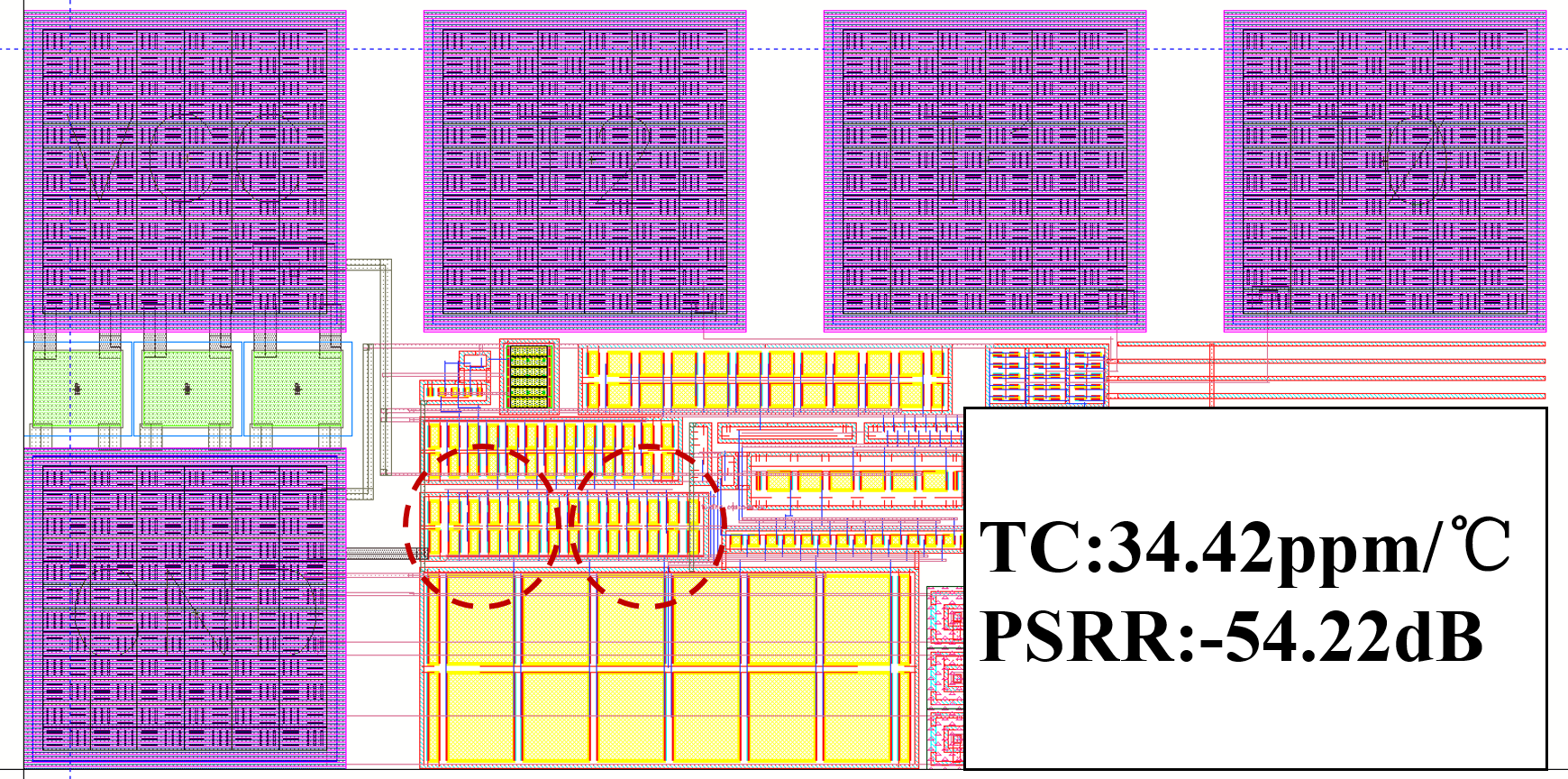
((a))

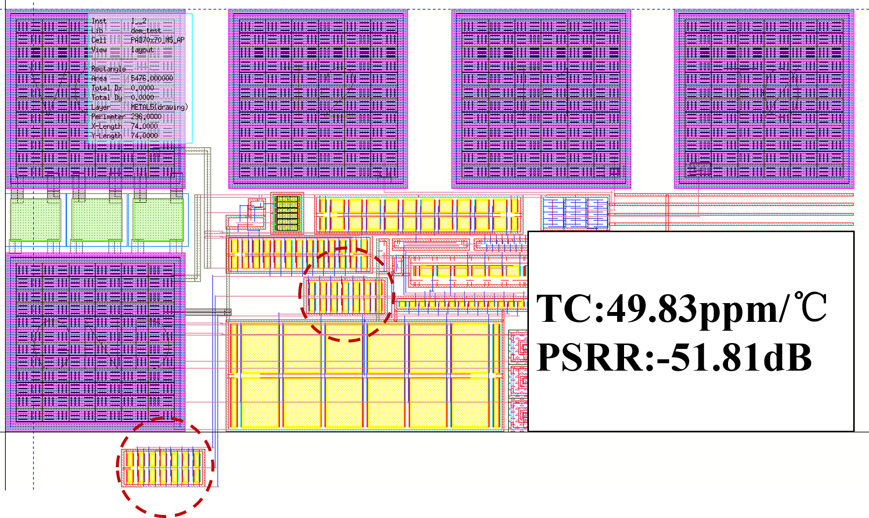
((b))

Figure 1: Layout of a Bandgap reference circuit with (a) accurate symmetric constraints and (b) a symmetric constraint removed.

With the development of artificial intelligence (AI) technology, there is a trend toward automated extraction of layout constraints for analog ICs based on deep learning algorithms. Kunal et al. [12] utilize a graph neural network (GNN) to handle multiple levels of symmetry hierarchies. However, the function of the GNN in the work is only to solve the graph edit distance (GED) to measure graph similarity, ignoring the adjacent topology at the device-level, and thus cannot effectively extract device-level constraints. The work [13] presents a simple and effective methodology to identify symmetric matching. It first represents device instances and corresponding pins in the circuit as nodes of a circuit graph, and then embeds the types of devices and pins as node features. Through training a GraphSAGE model [14], adjacent information is aggregated into node embeddings, which are adopted to identify whether two nodes are symmetric. Although the approach improves the accuracy of symmetry constraint extraction, it cannot detect the unpaired constraints with more than two devices, which is not reasonable in analog circuits. Besides, Chen et al. [15] propose a gated graph neural network (GGNN)-based method leveraging unsupervised learning to detect symmetric constraints in analog circuits. Since the GGNN aggregates neighboring node features with the convolution operation, the final embedding of each node contains information from its neighboring sub-graph. Based on the node embedding, the cosine similarity of the two nodes is computed as a criterion for symmetry. But the circuit netlist is converted as a heterogeneous directed multigraph, and the computation overhead of the GGNN is tremendously high.

To address these issues, we propose a novel graph-based learning framework to automatically extract layout constraints of analog circuits. Since the edges in netlist graph have different pin connections, an edge-augmented graph attention network (EGAT) is proposed to extract the netlist information. Compared with the traditional graph neural network, which focuses on node-level features, the proposed EGAT pays more attention to the interaction with node and edge features. By utilizing graph neural networks, our framework can analyze existing circuits and learn general rules of symmetry constraints, which in turn generalizes to new unseen circuits. Our main contributions are summarized as follows:

• An edge-augmented graph attention network (EGAT)-based learning framework is proposed to extract the netlist information effectively and measure the similarity of paired devices according to the resulting embeddings.

• A new graph representation for an analog circuit is built to model various analog circuit elements.

• Suitable circuit features are designed to realize information interaction with nodes and edges. Meanwhile, an extra feature is introduced to distinguish differential pairs and current mirrors in analog circuits.

• Several post-processing rules are developed to significantly reduce the false positive rate.

• Experimental results on typical analog circuit datasets demonstrate that the proposed graph learning framework achieves $>93\%$ TPR and $<1\%$ FPR, significantly outperforming S³DET-dl [11] and the recent GNN-based extraction approach [13] by a large margin.

The rest of the paper is organized as follows. Section II gives the preliminaries and formulates the symmetric constraint extraction problem. Section III describes the details of our proposed graph learning framework. Section IV presents the experimental results, followed by the conclusions in Section V.

II Preliminaries

In this section, the backgrounds of symmetric constraints in analog circuit layouts and graph neural networks are offered, and then we give the problem formulation.

II-A Symmetric Constraints in Analog Circuit Layout

In analog circuit systems, layout symmetry constraints significantly impact circuit performance. Based on the simple fact that the circuit netlist is a graph, we represent the netlist of an analog circuit as a directed graph $G=(V,E)$. $V$ denotes the nodes in the graph, representing circuit devices such as resistors, capacitors, transistors, etc., while $E$ describes the interconnection relationships among devices. For any pairwise combination, we need to detect the symmetrical device pair $(v_{i},v_{j})$ ($v_{i},v_{j}\in V$), which should be placed symmetrically on the centerline of the layout. Fig. 2 depicts a typical operational transconductance amplifier (OTA) circuit consisting of multiple pairs of symmetrically matched devices, i.e., $(v_{0},v_{1},v_{2})$, $(v_{3},v_{4})$, $(v_{5},v_{6},v_{7})$, $(v_{8},v_{9})$, $(v_{10},v_{11})$, $(v_{12},v_{13})$, $(v_{15},v_{16})$, and $(v_{17},v_{18},v_{20},v_{21})$.

Figure 2: A typical OTA circuit.

II-B Graph Neural Network

In recent years, traditional deep learning methods have achieved great success in extracting features from Euclidean space data. However, there exists a large number of practical application scenarios, where data are generated from non-Euclidean domains and are represented as graphs with complex relationships and interdependency between objects. To handle the complexity of graph data, the graph neural network is developed over the past few years. For example, graph convolutional network (GCN) [16] promotes convolutional operations from traditional data, such as images, to graph data. The main idea is to generate the representation of a node $v_{i}$ by aggregating its own features with its neighbors’ features. The GCN model is the basis of many complex graph neural network structures, including GraphSAGE network [14] and graph generative networks [17]. But different from the GCN model, the GraphSAGE network adopts sampling to achieve a fixed number of neighbors for each node. As a result, the efficiency of information interaction is improved.

In many sequence-based tasks, attention mechanisms have become almost de facto standards, which allow the model to focus on the most relevant parts of the input to make decisions. When an attention mechanism is adopted to calculate a representation of a single sequence, it is considered as a self-attention [18]. Based on the attention mechanism, graph attention network (GAT) [19] is developed to learn the relative weights between two connected nodes. Besides, in order to increase the expressive capability of the GAT model, the multi-head attention is performed for the node embeddings. Fig. 3 depicts the simple aggregation process in GAT network. But the traditional GAT model only focuses on node-level features and cannot achieve feature interaction between nodes and edges. To tackle the problem, an edge channel is introduced in [20] to explicitly obtain the structural information of a graph. Inspired by [18] and [20], an edge-augmented graph attention network (EGAT)-based learning framework is proposed in this work to pay more attention to the interaction with node and edge features.

Figure 3: The illustration of the graph attention mechanism on node 0 with its neighborhood, where $\bm{n}_{i}$ denotes the feature of node $i$. Different arrow colors and styles refer to independent attention computations (multi-head process). Based on the calculated attention score $s_{0j}$, the feature of the neighboring node $j$ is aggregated in node 0. Then, the aggregated features in each head are concatenated or averaged to achieve the final embedding $\hat{\bm{n}_{0}}$.

II-C Problem Formulation

In this work, we formulate the symmetric constraint extraction as a binary classification problem. Several comprehensive measurements are defined to evaluate the detection quality, including true positive rate (TPR), false positive rate (FPR), positive predictive value (PPV), accuracy (ACC), and F₁-score.

Definition 1 (TPR).

TPR is the number of true positive results divided by the number of all positive results as:

$$\textrm{TPR}=\frac{\textrm{TP}}{\textrm{TP}+\textrm{FN}}$$ (1)

where TP and FN are the number of the true positive and the false negative results.

Definition 2 (FPR).

FPR is the number of false positive results divided by the number of all negative results as:

$$\textrm{FPR}=\frac{\textrm{FP}}{\textrm{FP}+\textrm{TN}}$$ (2)

where FP and TN denote the number of the false positive and the true negative results.

Definition 3 (PPV).

PPV is the number of true positive results divided by the number of all predicted positive results as:

$$\textrm{PPV}=\frac{\textrm{TP}}{\textrm{TP}+\textrm{FP}}$$ (3)

Definition 4 (ACC).

ACC measures the proportion of correctly predicted samples to all samples, representing the overall accuracy of the prediction.

$$\textrm{ACC}=\frac{\textrm{TP}+\textrm{TN}}{\textrm{TP}+\textrm{FP}+\textrm{TN}+\textrm{FN}}$$ (4)

Definition 5 (F₁-score).

F₁-score reflects the balance of the model in positive and negative case classification.

$$\textrm{F}_{1}=\frac{2\textrm{TP}}{2\textrm{TP}+\textrm{FP}+\textrm{FN}}$$ (5)

Based on the above metrics, we define the symmetric constraint extraction problem as follows.

Problem 1 (Symmetric Constraint Extraction).

Given that various analog circuit netlists are labeled with symmetry pairs, the goal is to train a graph learning model to detect the symmetry pairs from the new circuit netlist, yielding higher TPR, PPV, ACC, F₁-scores, and lower FPR.

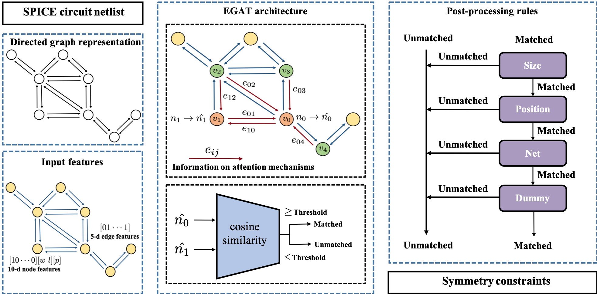
Figure 4: The diagram of the proposed EGAT-based symmetry constraint extraction framework.

III Proposed Graph Learning Framework

To extract symmetric constraints in analog circuits, we propose a graph learning-based framework as illustrated in Fig. 4, which consists of four main components, namely 1) directed graph representation, 2) input features, 3) edge-augmented graph attention network (EGAT) architecture, and 4) post-processing rules. In the directed graph representation stage, we convert the analog circuit netlist into a graph with bi-directional edges. Then, we utilize partial information of the devices (type, size, etc.) as node features and embed the connection relationship of the devices as edge features, which are then fed to the EGAT network architecture. Next, the proposed EGAT network effectively generates node embeddings, which are adopted to predict the probabilities of symmetry constraint. Finally, in the post-processing stage, several processing rules are designed to rectify the potential symmetry pair errors in EGAT recognition to improve accuracy. The detailed techniques are described below.

III-A Directed Graph Representation

In this section, we first explain how to represent a SPICE circuit netlist as a directed graph. For analog circuits, devices and IO ports are nodes of the graph, while the nets connecting devices or IO ports are recognized as edges. For a partial structure of the OTA circuit in Fig. 2 (blue dashed lines), $v_{3}$, $v_{4}$, $v_{8}$, and $v_{9}$ are the devices, $V_{dd}$ is the power IO port, and $net_{0}$, $net_{1}$, $net_{2}$, and $net_{3}$ refer to the nets. Since different connection directions between nodes indicate varying connection information, bi-directional edges between any two nodes are constructed in the graph. The corresponding directed graph representation is depicted in Fig. 5.

III-B Input Features

After the directed graph construction, we define an initial feature vector for each node. Since the size and type of the node are important factors for effectively identifying symmetric constraints, we convert the node type (i.e., NMOS, PMOS, NPN, PNP, diode, passive, IO) into a unique one-hot representation of a 7-dimensional vector. Moreover, the size information (length and width) of the node is represented as a 2-dimensional vector. Note that, the IO node’s size is set to a default value of -1, while the sizes of other nodes are normalized with values between [0,1]. Because many differential pairs and current mirrors exist in the analog circuit, and the main difference between them is the connection relation of the gates, an extra 1-dimensional feature is introduced to make the network perceive the connection difference. The 1-dimensional feature is set to 1 when the gate port of the node is connected to the IO port and 0 otherwise. After obtaining the vector representations of three parts, we concatenate them into a 10-dimensional vector as the final node feature. In addition, a 5-dimensional multi-hot vector is encoded for edges to represent the connection information. The first four dimensions indicate the connections to the gate port, drain port, source port of MOS, and passive device, while the last dimension denotes other possible pin connections (NPN, PNP, etc.). Fig. 5 illustrates the construction process of edge features. For example, node $v_{3}$ connects to the gate port of node $v_{4}$, and thus the feature for the edge from node $v_{3}$ pointing to $v_{4}$ is [1,0,0,0,0]. Table I summarizes the initial features and dimensions of nodes and edges, which are concatenated into vector representations and then passed to the downstream graph network.

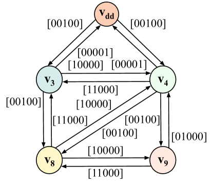
Figure 5: The directed graph representation for the partial circuit structure in Fig. 2. The edge connections are as follows: node $v_{3}$ is connected to the gate port of node $v_{4}$, the source port of node $v_{8}$, and the power port $V_{dd}$; node $v_{4}$ is connected to the gate and drain ports of node $v_{3}$, the source ports of nodes $v_{8}$ and $v_{9}$, and the power port $V_{dd}$; node $v_{8}$ is connected to the gate and drain ports of node $v_{3}$, and the gate ports of nodes $v_{4}$ and $v_{9}$; node $v_{9}$ is connected to the drain port of node $v_{4}$, and the gate and drain ports of node $v_{8}$.

TABLE I: Designed features of nodes and edges in the directed graph representing the analog circuit netlist.

Type	Feature Description	Dimension
Node	One-hot representation for device type	7
	Length and width of device	2
	Connection relationship of gate port	1
Edge	Connection information between pins	5

III-C EGAT Architecture

Based on the input node and edge features, the developed EGAT network further extracts the embeddings of nodes and edges. In order to increase the expressive capability of the model, an edge-augmented attention mechanism is performed for each node. Each layer $l$ in the EGAT consists of four calculation processes: layer normalization, attention score calculation, node embedding update, and edge embedding update, as shown in Fig. 6.

Layer Normalization (LN) [21] plays a crucial role in standardizing inputs, avoiding the exploding or vanishing gradients, and accelerating the training process. The calculation process of LN is as follows.

$$\mu^{l}=\frac{1}{{n}^{l}}\sum_{i=1}^{{n}^{l}}{x_{i}}^{l},\ (\sigma^{l})^{2}=\frac{1}{{n}^{l}}\sum_{i=1}^{{n}^{l}}({x_{i}}^{l}-\mu^{l})^{2},$$ (6)

$$\bm{\hat{x}}^{l}=\frac{\bm{x}^{l}-\mu^{l}}{\sqrt{(\sigma^{l})^{2}+\epsilon}},\ \mathrm{LN}_{\bm{\alpha},\bm{\beta}}(\bm{x}^{l})=\bm{\alpha}\odot\bm{\hat{x}}^{l}+\bm{\beta},$$

where $\bm{x}^{l}$ is the input of the $l$-th layer, and $n^{l}$ refers to the number of neurons in the $l$-th layer. $\mu^{l}$ and $\sigma^{l}$ represent the mean and the standard deviation of the input data, respectively. Besides, $\epsilon$ is a small constant, while $\bm{\alpha}$ and $\bm{\beta}$ are learnable parameters with the same dimension as $\bm{x}^{l}$. $\odot$ is the Hadamard product. In this work, we first perform the LN on the initial features as follows.

$$\bm{\hat{n}}^{l}=\mathrm{LN}_{\bm{\alpha},\bm{\beta}}(\bm{n}^{l}),\ \ \bm{\hat{e}}^{l}=\mathrm{LN}_{\bm{\alpha},\bm{\beta}}(\bm{e}^{l}),$$ (7)

where $\bm{n}^{l}$ and $\bm{e}^{l}$ are the embeddings of all nodes and edges in the $l$-th layer. As the $\mathrm{LN}$ technique enables the model to adapt to various inputs, the model can generalize to new unseen netlists.

Then the multi-head attention mechanism is performed over the learned node representations produced by $\mathrm{LN}$. The attention score of node $v_{i}$ with its neighbouring node $v_{j}$ are computed as follows.

$$\bm{a}_{ij}^{l}=\mathrm{reshape}((\bm{W}_{i}^{l}\hat{\bm{n}}_{i}^{l})\odot({\bm{W}_{j}^{l}}\hat{\bm{n}}_{j}^{l}))+\bm{W}_{e}^{l}\hat{\bm{e}}_{ij}^{l},$$ (8)

$$s_{ij}^{l}=\frac{\mathrm{exp}{(\bm{b}^{l^{\top}}\bm{a}_{ij}^{l})}}{\sum\limits_{j\in\mathcal{N}_{i}}{\mathrm{exp}(\bm{b}^{l^{\top}}\bm{a}_{ij}^{l})}},$$

where $\hat{\bm{n}}_{i}^{l}\in{\mathbb{R}^{d_{n}}}$, $\hat{\bm{n}}_{j}^{l}\in{\mathbb{R}^{d_{n}}}$ and $\hat{\bm{e}}_{ij}^{l}\in{\mathbb{R}^{d_{e}}}$ are the embeddings of node $v_{i}$, node $v_{j}$ and the corresponding edge. $\bm{W}_{i}^{l}\in{\mathbb{R}^{d_{n}\times d_{n}}}$, $\bm{W}_{j}^{l}\in{\mathbb{R}^{d_{n}\times d_{n}}}$, $\bm{W}_{e}^{l}\in{\mathbb{R}^{d_{e}\times d_{e}}}$ and $\bm{b}^{l}\in{\mathbb{R}^{d_{e}}}$ denote learning parameters. $\mathrm{reshape}(\cdot)$ refers to the reshape operations. Besides, $\mathcal{N}_{i}$ represents the neighborhoods of node $v_{i}$ in the graph. In reality, due to the multi-head attention mechanism, the above calculation is decomposed in multiple heads. The calculated attention score $s_{ij}^{l}$ indicates the importance of node $v_{j}$’s embedding to node $v_{i}$.

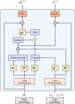
Figure 6: The architecture of the EGAT network.

On the basis of the attention scores, the node embeddings are updated by the weighted average pooling operation. To further enhance the representation ability of the model, we use an MLP to carry out the non-linear transformation of the pooled node embeddings. Besides, the residual connection is performed to facilitate training networks [22]. The final node representation is updated as:

$$\bm{n}_{i}^{l+1}=\mathrm{MLP_{n}}(\bm{n}_{i}^{l}+\widetilde{\bm{W}}^{l}\sum_{j\in\mathcal{N}_{i}}{s_{ij}^{l}\cdot\mathrm{concat}(\bm{W}_{k}^{l}\hat{\bm{n}}_{j}^{l},\widehat{\bm{W}}_{e}^{l}\hat{\bm{e}}_{ij}^{l})}),\\$$ (9)

where $\bm{W}_{k}^{l}\in{\mathbb{R}^{d_{n}\times d_{n}}}$, $\widehat{\bm{W}}_{e}^{l}\in{\mathbb{R}^{d_{e}\times d_{e}}}$ and $\widetilde{\bm{W}}^{l}\in{\mathbb{R}^{(d_{n}+d_{e})\times d_{n}}}$ refer to learning weight vectors. $\mathrm{concat}(\cdot)$ represents the concatenation operation. $\mathrm{MLP_{n}}(\cdot)$ denotes a non-linear transformation with input dimension $d_{n}$ and output dimension $d_{n}$.

Similarly, the edge representation is also updated with a residual connection as follows:

$$\bm{e}_{ij}^{l+1}=\mathrm{MLP_{e}}(\bm{e}_{ij}^{l}+\bm{a}_{ij}^{l}),$$ (10)

where $\mathrm{MLP_{e}}(\cdot)$ refers to another non-linear transformation with input dimension $d_{e}$ and output dimension $d_{e}$, and $\bm{a}_{ij}^{l}$ is the intermediate feature calculated in Equation 8.

As demonstrated above, the proposed EGAT network differs from the traditional attention method in GAT network [19] in that edge features are introduced to calculate attention scores, which are further adopted to update both node and edge features. As a result, the information interactions between nodes and edges are realized. Since the edge features reflect the pin connectivity between nodes, by incorporating the edge feature into the calculation of the attention score, the symmetric matching pairs can be distinguished effectively. Therefore, EGAT makes full use of the characteristics of the netlist graph for the symmetric constraint extraction in analog circuits.

Based on the node embeddings generated by the EGAT architecture, we should provide a predicted similarity score for each candidate symmetry pair $(v_{i},v_{j})$ ($v_{i},v_{j}\in V$). As the symmetric constraint extraction is formulated as a binary classification problem, labels are annotated in advance, where the symmetric and asymmetric node pairs are labeled as 1 and -1 respectively. To match with the labels, the $\mathrm{cosine}$ similarity function is adopted to predict the probabilities of symmetry constraint.

$$\mathrm{similarity}=\frac{\bm{n}_{i}\cdot\bm{n}_{j}}{|\bm{n}_{j}||\bm{n}_{j}|},$$ (11)

where $\bm{n}_{i}$ and $\bm{n}_{j}$ are the embeddings of nodes $v_{i}$ and $v_{j}$ produced by the EGAT.

Due to the utilization of the $\mathrm{cosine}$ similarity function, the binary cross-entropy loss [23] originally used to infer results in the range [0,1] is no longer valid. To accommodate this, the logistics loss function is employed for the output label with 1 and -1 as:

$$loss=\log{(1+e^{-gs})},$$ (12)

where $gs$ is the product of the ground truth and the similarity score, which reflects the accuracy and the confidence level of prediction. That is, when $gs\geq 0$, the prediction is correct, and the larger the value, the higher the confidence level. On the contrary, when $gs<0$, the prediction is incorrect, and the smaller the value, the lower the confidence level.

Algorithm 1 The Pseudo-code of Device Position Calculation

Input: A directed graph $G$ for a circuit.

Output: The position $p_{n}$ of each device.

1:              $\triangleright$ Assign weights for edges

2:for each edge $e$ in $G$ do

3:     Get two devices connected by $e$ as $d_{i}$ and $d_{j}$;

4:     if $d_{i}$ and $d_{j}$ are passive devices then

5:         Set the weight of $e$ to 0;

6:     else if $d_{i}$ or $d_{j}$ is a passive device then

7:         Set the weight of $e$ to 0.5;

8:     else

9:         Set the weight of $e$ to 1;

10:     end if

11:end for

12:              $\triangleright$ Find the device position

13:for each node $n$ in $G$ do

14:     if $n$ is a PMOS then

15:         Calculate the shortest path from Power node to $n$;

16:         $p_{n}$ = the weighted length of the path;

17:     else if $n$ is a NMOS then

18:         Calculate the shortest path from GND node to $n$;

19:         $p_{n}$ = the weighted length of the path;

20:     else

21:         $p_{n}$ = $0$.

22:     end if

23:end for

III-D Post-Processing Rules

Although the graph learning framework can annotate the symmetry constraints, a case still exists where asymmetric pairs are identified as symmetry constraints. Thus, we further develop several post-processing rules to reduce the false positive rate (FPR).

The first rule is that the symmetric pairs must have the same type and size. Although the designed features of nodes in the neural network contain the type and size information, some device pairs with varying sizes are incorrectly recognized as symmetric pairs after the EGAT recognition. Thus, the first post-processing rule can rectify the potential symmetry pair errors.

Moreover, we observe that symmetric device pairs tend to have identical device positions, as defined below.

Definition 6 (Device Position).

For each PMOS device, we find the shortest path from the Power node to the device. Conversely, for each NMOS device, the shortest path from the GND node to the device is calculated. The weighted length of the shortest path refers to the device position.

Algorithm 1 depicts the process of determining the positions of the devices in an analog circuit. Fig. 7 shows the device positions of the OTA circuit in Fig. 2. It can be seen that symmetric devices exhibit the same device positions.

Additionally, based on the fact that devices lacking a shared net connection cannot be matched, another post-processing rule is designed to eliminate wrongly identified symmetric pairs without shared nets.

Finally, dummies are generally added to reduce the mismatch between transistor pairs or fill in missing parts of the layout. Thus, dummies contain no actual functionality and are designed purely for the performance and stability of the circuit layout, which are also unnecessary constraints that we need to eliminate.

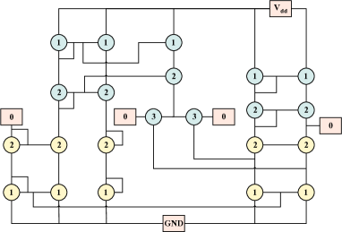
Figure 7: The illustration of device positions, where the green and yellow circles represent PMOS and NMOS devices and the pink rectangle denotes IO ports.

IV Experimental Results

IV-A Simulation Setup

The proposed graph learning framework is implemented in Python with the Pytorch library [24], and we execute it on a Linux server with the Intel Xeon Gold 6254 CPU and Nvidia Tesla V100 GPU. The proposed EGAT architecture includes a three-layer network with five attention heads. The threshold for the similarity score calculated in Equation 11 is set to 0.6. That is, if the similarity score of a valid pair is greater than 0.6, the pair will be annotated as a symmetry constraint. Unlike the most commonly used threshold of 0.9 or higher, the low threshold ensures that more symmetric pairs are correctly identified, despite potentially resulting in a higher false alarm rate. But the developed post-processing can effectively eliminate these misidentified pairs. During the training, each batch consists of 256 valid pairs. Besides, the adaptive moment estimation (Adam) optimizer [25] is adopted to train the network models. We will release the detailed codes soon.

IV-B Dataset Generation

To demonstrate the effectiveness and scalability of our proposed graph learning framework, we conduct comprehensive experiments on real-world analog circuits. Specifically, 20 circuits are designed by experienced analog engineers under TSMC 180$nm$ technology, covering various functional types, including operational transconductance amplifier (OTA), comparator (COMP), and bandgap reference circuit. The OTA circuit is commonly employed as a signal-processing component and is widely used in analog front-end applications. The COMP circuit facilitates comparison between analog and reference signals, subsequently generating digital signals or switching control signals based on the comparison results. The COMP circuit is valued for its high speed, accuracy, and common mode rejection ratio (CMRR), and its device parameters significantly impact the performance of the entire circuit. A Bandgap reference circuit is designed to provide precise and PVT (process, supply voltage, temperature) insensitive reference voltages, which is a critical component in analog circuit design.

Based on these 20 circuits, two datasets are constructed, the first of which contains all circuits named Hybrid, while the second includes only the OTA circuits denoted OTA. As described in Section III-A, the SPICE circuit netlist can be represented as a directed graph, where devices and IO ports are nodes, and the nets are recognized as edges. We extract all the necessary information from the SPICE files to generate graph feature embeddings. In our dataset, we define a valid pair as one that matches the type rule. In addition, we roughly divide each dataset into training and testing sets in a 3:1 ratio at the circuit level. The graph learning-based model is trained only on the training set. This ensures that the tested circuits are totally unseen to the network model, eliminating the possibility of information leaking from the testing set to the training set. The statistics on the circuit graphs are listed in Table II.

TABLE II: Statistics of the datasets.

Dataset	#Circuits	#Nodes	#Edges	#Valid pairs
Hybrid	20	724	4916	3768
OTA	15	496	3208	2817

IV-C Baselines Description

To verify the superiority of the proposed framework, we compare our framework with two state-of-the-art symmetric constraint detection methods, including S³DET [11] and ASPDAC’21 [13]. The S³DET algorithm leverages spectral graph analysis and graph centrality to detect system-level symmetry constraints. Thanks to the modifications by Lin et al. [13], the algorithm adapts to the device-level symmetry constraint detection, subsequently renaming it S³DET-dl. In ASPDAC’21, a GraphSAGE model is exploited to aggregate adjacent information into node embeddings, which are adopted to identify whether two nodes are symmetric.

IV-D Comparison with Baselines

We compare our framework with S³DET-dl [11] and ASPDAC’21 [13] on the two datasets. To ensure a fair comparison, all the parameters of the SOTA works are set the same as those in these original papers. Table III lists the experimental results. The evaluation metrics TPR, FPR, PPV, ACC, and F₁-score are defined in Section II-C. Column “Training time” represents the total training time on all training circuits. Meanwhile, column “Inference time” denotes the average inference time on each tested circuit, which also contains the post-processing time. We emphasize the better results in bold. As shown in the table, the proposed EGAT framework significantly outperforms S³DET-dl and ASPDAC’21 in all metrics. For example, compared with ASPDAC’21, the proposed EGAT improves the TPR, PPV, ACC, and F₁-score by $19.49\%$, $49.77\%$, $13.68\%$, and $38.25\%$, respectively, while the FPR is reduced by $12.89\%$ on the Hybrid dataset. Meanwhile, on the OTA dataset, the proposed EGAT framework achieves $100\%$ TPR and $99.8\%$ ACC. Moreover, the training and inference time expenses are still less than those of S³DET-dl and ASPDAC’21. In the layout automation of analog circuits, constraint extraction is the first stage where higher TPR and lower FPR values can alleviate the difficulties and computational costs of the subsequent placement and routing, significantly reducing the overall design complexity. More importantly, since the circuits vary considerably in Hybrid and OTA datasets, the experimental results also demonstrate that our framework can generalize to different types of analog circuits.

TABLE III: Comparison with state of the arts on Hybrid and OTA datasets (time unit: $s$).

Dataset	Model	TPR	FPR	PPV	ACC	F1 score	Training time	Inference time
Hybrid	S3DET-dl [11]	0.7019	0.4110	0.3676	0.6176	0.3254	-	0.6185
	ASPDAC’21 [13]	0.7404	0.1383	0.4470	0.8457	0.5575	320.52	0.1434
	EGAT	0.9353	0.0094	0.9447	0.9825	0.9400	61.04	0.0621
OTA	S3DET-dl [11]	0.4498	0.2732	0.3068	0.6680	0.2673	-	0.6515
	ASPDAC’21 [13]	0.9063	0.1891	0.3480	0.8204	0.5028	317.19	0.1221
	EGAT	1.0000	0.0021	0.9804	0.9980	0.9901	55.11	0.1189

IV-E Ablation Study

An ablation study is performed to investigate how different post-processing rules affect the performance. Fig. 8 summarizes the contribution of the post-processing rules. “EGAT” represents the framework without any post-processing rules, “R₁” refers to the framework only with the size-based rule, “R_1,2” stands for the framework with the size-based and device position rules, “R_1,2,3” denotes the framework without the dummy-based rule, while “Full” is our framework with entire post-processing rules. The histogram shows that comparing the framework only with EGAT model, the post-processing rules reduce 10.68% of the false positive rate and get 9.05% further improvement on accuracy.

Another ablation study is performed on the graph learning framework to investigate how the number of network layers in the EGAT model affects the performance. Fig. 9 records the changes of TPR and F₁-score on the Hybrid dataset with respect to the model’s layer numbers. As illustrated in the histogram, with the network depth increasing, TPR and F₁-score get saturated and then decreases gradually. Thus, it is reasonable to set the layer numbers of the EGAT model to 3.

Figure 8: Comparisons of (a) ACC and (b) FPR of different post-processing rules (Hybrid dataset).

Figure 9: Comparisons of (a) TPR and (b) F₁-score of different layer numbers of the EGAT model (Hybrid dataset).

V Conclusion

In this paper, we have proposed a graph learning framework to automatically extract symmetric constraints in analog circuits, which effectively combines edge information in a graph with attentional mechanisms. Suitable circuit features are designed to guide the network model to achieve information interaction with devices. Besides, several post-processing rules are developed to significantly reduce the false positive rate. Experimental results show that, compared with the SOTA implementations, our approach produces better performance. In the future, we will extend the framework to recognize system-level symmetries in analog circuits.

References

- [1] U. Choudhury and A. Sangiovanni-Vincentelli, “Constraint generation for routing analog circuits,” in ACM/IEEE Design Automation Conference (DAC), 1991, pp. 561–566.
- [2] E. Malavasi, E. Charbon, E. Felt, and A. Sangiovanni-Vincentelli, “Automation of ic layout with analog constraints,” IEEE Transactions on Computer-Aided Design of Integrated Circuits and Systems (TCAD), vol. 15, no. 8, pp. 923–942, 1996.
- [3] E. Charbon, E. Malavasi, and A. Sangiovanni-Vincentelli, “Generalized constraint generation for analog circuit design,” in IEEE/ACM International Conference on Computer-Aided Design (ICCAD), 1993, pp. 408–414.
- [4] S. Bhattacharya, N. Jangkrajarng, R. Hartono, and C.-J. Shi, “Hierarchical extraction and verification of symmetry constraints for analog layout automation,” in IEEE/ACM Asia and South Pacific Design Automation Conference (ASPDAC). IEEE, 2004, pp. 400–405.
- [5] P.-H. Wu, M. P.-H. Lin, T.-C. Chen, C.-F. Yeh, X. Li, and T.-Y. Ho, “A novel analog physical synthesis methodology integrating existent design expertise,” IEEE Transactions on Computer-Aided Design of Integrated Circuits and Systems (TCAD), vol. 34, no. 2, pp. 199–212, 2014.
- [6] P.-H. Wu, M. P.-H. Lin, and T.-Y. Ho, “Analog layout synthesis with knowledge mining,” in European Conference on Circuit Theory and Design (ECCTD), 2015, pp. 1–4.
- [7] Q. Hao, S. Chen, X. Hong, Y. Su, S. Dong, and Z. Qu, “Constraints generation for analog circuits layout,” in International Conference on Communications, Circuits and Systems (ICCCAS), 2004, pp. 1334–1338.
- [8] Z. Zhou, S. Dong, X. Hong, Q. Hao, and S. Chen, “Analog constraints extraction based on the signal flow analysis,” in International Conference on ASIC (ASICON), 2005, pp. 825–828.
- [9] T. Massier, H. Graeb, and U. Schlichtmann, “The sizing rules method for CMOS and bipolar analog integrated circuit synthesis,” IEEE Transactions on Computer-Aided Design of Integrated Circuits and Systems (TCAD), vol. 27, no. 12, pp. 2209–2222, 2008.
- [10] M. Eick, M. Strasser, K. Lu, U. Schlichtmann, and H. E. Graeb, “Comprehensive generation of hierarchical placement rules for analog integrated circuits,” IEEE Transactions on Computer-Aided Design of Integrated Circuits and Systems (TCAD), vol. 30, no. 2, pp. 180–193, 2011.
- [11] M. Liu, W. Li, K. Zhu, B. Xu, Y. Lin, L. Shen, X. Tang, N. Sun, and D. Z. Pan, “DET: Detecting system symmetry constraints for analog circuits with graph similarity,” in IEEE/ACM Asia and South Pacific Design Automation Conference (ASPDAC), 2020, pp. 193–198.
- [12] K. Kunal, J. Poojary, T. Dhar, M. Madhusudan, R. Harjani, and S. S. Sapatnekar, “A general approach for identifying hierarchical symmetry constraints for analog circuit layout,” in IEEE/ACM International Conference on Computer-Aided Design (ICCAD), 2020, pp. 1–8.
- [13] X. Gao, C. Deng, M. Liu, Z. Zhang, D. Z. Pan, and Y. Lin, “Layout symmetry annotation for analog circuits with graph neural networks,” in IEEE/ACM Asia and South Pacific Design Automation Conference (ASPDAC), 2021, pp. 152–157.
- [14] W. Hamilton, Z. Ying, and J. Leskovec, “Inductive representation learning on large graphs,” in Conference on Neural Information Processing Systems (NIPS), 2017, pp. 1025–1035.
- [15] H. Chen, K. Zhu, M. Liu, X. Tang, N. Sun, and D. Z. Pan, “Universal symmetry constraint extraction for analog and mixed-signal circuits with graph neural networks,” in ACM/IEEE Design Automation Conference (DAC), 2021, pp. 1243–1248.
- [16] T. N. Kipf and M. Welling, “Semi-supervised classification with graph convolutional networks,” arXiv preprint arXiv:1609.02907, 2016.
- [17] M. Simonovsky and N. Komodakis, “GraphVAE: Towards generation of small graphs using variational autoencoders,” in International Conference on Artificial Neural Networks (ICANN), 2018, pp. 412–422.
- [18] A. Vaswani, N. Shazeer, N. Parmar, J. Uszkoreit, L. Jones, A. N. Gomez, Ł. Kaiser, and I. Polosukhin, “Attention is all you need,” in Conference on Neural Information Processing Systems (NIPS), 2017, pp. 1–11.
- [19] P. Veličković, G. Cucurull, A. Casanova, A. Romero, P. Lio, and Y. Bengio, “Graph attention networks,” arXiv preprint arXiv:1710.10903, 2017.
- [20] M. S. Hussain, M. J. Zaki, and D. Subramanian, “Global self-attention as a replacement for graph convolution,” in ACM International Conference on Knowledge Discovery and Data Mining (KDD), 2022, pp. 655–665.
- [21] J. L. Ba, J. R. Kiros, and G. E. Hinton, “Layer normalization,” arXiv preprint arXiv:1607.06450, 2016.
- [22] K. He, X. Zhang, S. Ren, and J. Sun, “Deep residual learning for image recognition,” in IEEE Conference on Computer Vision and Pattern Recognition (CVPR), 2016, pp. 770–778.
- [23] C. M. Bishop and N. M. Nasrabadi, Pattern recognition and machine learning. Springer, 2006, vol. 4, no. 4.
- [24] A. Paszke, S. Gross, S. Chintala, G. Chanan, E. Yang, Z. DeVito, Z. Lin, A. Desmaison, L. Antiga, and A. Lerer, “Automatic differentiation in PyTorch,” in NIPS Workshop, 2017.
- [25] D. P. Kingma and J. Ba, “Adam: a method for stochastic optimization,” arXiv preprint arXiv:1412.6980, 2014.