Constraint-Informed Learning for Warm Starting Trajectory Optimization

Abstract

Future spacecraft and surface robotic missions require increasingly capable autonomy stacks for exploring challenging and unstructured domains and trajectory optimization will be a cornerstone of such autonomy stacks. However, the nonlinear optimization solvers required remain too slow for use on relatively resource constrained flight-grade computers. In this work, we turn towards amortized optimization, a learning-based technique for accelerating optimization run times, and present TOAST: Trajectory Optimization with Merit Function Warm Starts. Offline, using data collected from a simulation, we train a neural network to learn a mapping to the full primal and dual solutions given the problem parameters. Crucially, we build upon recent results from decision-focused learning and present a set of decision-focused loss functions using the notion of merit functions for optimization problems. We show that training networks with such constraint-informed losses can better encode the structure of the trajectory optimization problem and jointly learn to reconstruct the primal-dual solution while also yielding improved constraint satisfaction. Through numerical experiments on a Lunar rover problem, we demonstrate that TOAST outperforms benchmark approaches in terms of both computation times and network prediction constraint satisfaction.

1 Introduction

Surface rovers have a rich history of use in planetary exploration and on-board autonomy has played a critical role in enabling new scientific discoveries. For example, Mars rover missions such as NASA’s Curiosity and Perseverance have driven tens of kilometers through their mission lifetimes and autonomous driving capabilities such as  Enhanced AutoNav (ENav) have played a crucial part in enabling the rovers to carry out valuable in situ measurements and scientific operations (Rankin et al., 2020; Verma et al., 2023). However, current rover missions operate at relatively low driving speeds, allowing ENav to utilize a simple search-based approach that outputs geometric paths without consideration to high-fidelity dynamics, state, and actuator constraints of the full system. Instead, future missions that call for operating at significantly faster speeds will require planners that include a trajectory optimization layer and allow for the rover to plan trajectories that fully satisfy kinodynamic constraints.

One bottleneck for aerospace applications is that despite the tremendous breakthroughs in on-board numerical optimization solvers, flight-grade computers are significantly resource constrained and typically lack the computing power to be able to solve trajectory optimization problems at the speeds required for real-time operation (Eren et al., 2017). In recent years, a promising approach that has emerged has been that of amortized optimization (Amos, 2023), an area of work that seeks to use data-driven methods to learn a problem-solution mapping and significantly reduce the runtimes required to solve challenging nonlinear optimization problems online. Despite this progress, one shortcoming of such amortized optimization methods is that they disregard the downstream physical and safety constraints of the control task while predicting solutions on-board. In this work, we seek to bridge this gap and develop an amortized optimization approach for solving trajectory optimization problems on resource-constrained planetary rover missions with the following desiderata in mind:

1. Performant: The controller should yield high quality or near optimal solutions with respect to some task metric.

2. Decision-focused: The amortized optimization approach should be cognizant of the constraints enforced by the controller downstream.

3. Generalizable: The solution approach should not be tailored to a specific problem formulation and be applicable to a host of future missions requiring on-board trajectory optimization.

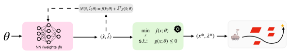
Figure 1: Schematic of the TOAST approach for learning warm starts using task-relevant merit functions. The problem parameters $\theta$ are used to make a prediction for the warm start to the optimization problem (shown in green). The neural network (shown in pink) with parameters $\phi$ used to generate this prediction is trained offline to minimize the task-relevant merit function associated with the optimization problem using offline data.

Related work: In recent years, there has been a flurry of work on applying data-driven and amortized optimization-based techniques, or learning to predict the solutions to similar instances of the same problem, for accelerating solution times for optimization problems (Kotary et al., 2021; Cauligi et al., 2022b). These techniques approach the problem of accelerating solution times for numerical optimization-based control through the lens of parametric programming, a technique to build a function $f:\theta\rightarrow x^{*}$ that maps the parameters, or context $\theta\subseteq\Theta$, of an optimization problem, $\mathcal{P}(\theta)$, to its solution, $x^{*}(\theta)\in{\mathbf{R}}^{n_{x}}$ (Dua et al., 2008). This is accomplished by sampling $\theta$ representative of the problems of interest, solving for the $x^{*}$ corresponding to these $\Theta$, and then training an approximation $\hat{f}$ via supervised learning (Amos, 2023).

Applications of amortized optimization have shown tremendous promise in the field of control. The authors in (Tang et al., 2018; Chen et al., 2022; Sambharya et al., 2023) propose using a neural network to warm start solutions for a  quadratic program (QP)-based  model predictive control (MPC) controller. Additional works have studied extensions for quickly solving non-convex optimal control problems online. In (Ichnowski et al., 2020), the authors train a neural network to learn the problem solution mapping for a non-convex robotic grasp optimization problem solved using  sequential quadratic programming (SQP). The authors in (Briden et al., 2024) train a transformer neural network to learn a mapping between problem parameters to the set of active tight constraints and final times and were shown to reduce solution times for a powered descent guidance problem by more than an order of magnitude. However, the problem formulations in these works neglect how the learned mapping is utilized and the provided warm starts are agnostic of the underlying structure of the trajectory optimization problem.

Statement of Contributions: In this work, we introduce Trajectory Optimization with Merit Function Warm Starts (TOAST), a framework designed to bridge the gap in the aforementioned fields of amortized optimization and nonlinear trajectory optimization. In the offline phase of the TOAST framework, a neural network is trained to map the problem parameters to the time-varying policy associated with a non-convex trajectory optimization problem. Crucially, this neural network is trained with a decision-focused loss function that jointly learns minimizing both the reconstruction error and the feasibility of the prediction by using the merit function associated with the underlying trajectory optimization problem. Online, the network is used to make a prediction for the full state and control trajectories for a new problem and this prediction used to warm start the trajectory optimization solver. We show through numerical simulations on a surface rover trajectory planning problem that our proposed TOAST approach outperforms benchmark amortized optimization approaches in terms of improved constraint satisfaction.

2 Preliminaries

2.1 Learning a Solution Map

Given a vector of problem parameters $\theta\in{\mathbf{R}}^{n_{p}}$, a parametric  optimal control problem (OCP) can be written as

$$\begin{array}[]{ll}\underset{x_{0:N},u_{0:N}}{\textrm{minimize}}\!\!\!&\sum_{t=0}^{N}g_{t}(x_{t},u_{t};\theta)\\ \text{subjectto}\!\!\!&x_{0}=x_{\textrm{init}}(\theta)\\ &x_{t+1}=\psi_{t}(x_{t},u_{t};\theta),\quad t=0,\dots,N-1\\ &f_{t,i}(x_{t},u_{t};\theta)\leq 0,\quad\;\;\;\,t=0,\dots,N,i=1,\dots,n_{\mathrm{f}},\\ \end{array}$$ (1)

where the state $x_{t}\in{\mathbf{R}}^{n_{x}}$ and control $u_{t}\in{\mathbf{R}}^{n_{u}}$ are the continuous decision variables. Here, the stage cost $g_{t}(\cdot)$ and terminal cost $g_{N}(\cdot)$ are assumed to be convex functions, but the dynamical constraints $\phi_{t}(\cdot)$ and inequality constraints $f_{t,i}(\cdot)$ are assumed smooth but possibly non-convex. The objective function and constraints are functions of the parameter vector $\theta\in\Theta$, where $\Theta\subseteq{\mathbf{R}}^{n_{p}}$ is the admissible set of parameters.

In the context of robotics, the OCP is typically solved in a receding horizon fashion as the controller replans periodically, wherein the problem size typically stays fixed, but only the problem parameters $\theta$ vary between repeated optimization calls. This setting motivates learning function $f$ that maps problem parameters $\theta$ to the optimal solution $x^{*}$ for the OCP, as the learned mapping can be utilized directly (e.g., imitation learning) or as a warm start initialization for the solver.

2.2 Decision-Focused Learning

Although amortized optimization has emerged as nascent area of research for improving the computational efficiency of optimal control problems, an often overlooked component of the supervised learning techniques used for amortized optimization is the loss function. The loss functions used in amortized optimization forgo utilizing the underlying structure of the trajectory optimization problem or solver. In this work, we seek to instead build upon recent contributions in the area of decision-focused learning (Wilder et al., 2019; Mandi et al., 2023). While learning based approaches typically use a traditional catalog of loss functions to train a neural network, decision-focused learning is a paradigm that integrates the learning with the usage or “decision making” of the model being deployed. To extend these approaches to amortized optimization, we turn to the solution techniques used for solving constrained optimization to formalize the concept of decision-focused losses and consider merit functions, which are a scalar-valued function of problem variables that indicates whether a new iterate is better or worse than the current iterate, with the goal of minimizing a given function (Nocedal and Wright, 2006). Although a candidate merit function for unconstrained optimization problems is simply the objective function, a merit function for a constrained optimization problem must balance the minimization of the cost function with a measure of constraint violation. For example, an admissible merit function for eq:nlp is the penalty function of the form $\phi(x,\mu)=f(x)+\mu\sum_{i\in\mathcal{E}}|c_{i}(x)|+\mu\sum_{i\in\mathcal{I}}[c_{i}(x)]^{-}$, where $[c_{i}(x)]^{-}=\max\{0,-c_{i}(x)\}$ (we refer the reader to (Nocedal and Wright, 2006) for a more exhaustive discussion and examples of merit functions). TOAST generalizes this definition of a merit function to develop a set of decision-focused loss function formulations to facilitate effective warm-starts for online MPC.

3 Technical Approach

In this work, we seek to learn a solution mapping $f(\theta)$ that maps problem parameters $\theta$ to the optimizer $z^{*}=(x^{*},u^{*})$, where $x$ are the state trajectories and $u$ are the control inputs. This can be accomplished by approximating the solution map $f(\theta)$ using a deep neural network $f_{\phi}(\theta)$, wherein $\phi$ are the neural network parameters to be learned. By formulating this problem as a parametric machine learning problem, a dataset $\mathcal{D}=((\theta_{i},z_{i}))_{i=1}^{n}$, a parameterized function class $f_{\phi}$, and a loss function $L(z,f_{\phi}(\theta))$ are user-specified and the goal of the learning framework is to compute $\phi$ such that the expected risk on unseen data is minimized, $\min_{\phi}\mathbb{E}[L(z,f_{\phi}(\theta))]$. Note that the minimum of the expected risk over unseen data cannot be computed, since we do not have access to all unseen data. Assuming the training set is a sufficient representation of the unseen data, $\min_{\phi}L(z,f_{\phi}(\theta))$, the empirical risk (training loss) will well-represent the expected risk (test loss).

If $\hat{z}$ denotes the full primal solution prediction $(\hat{x},\hat{u})$, then the “vanilla” approach to accomplish this would be to simply model $f_{\phi}(\cdot)$ as a regressor and output a prediction $\hat{z}$ for the full primal solution, i.e., $f_{\phi}(\theta)=\hat{z}$. However, this approach has the shortcoming that predicting the full primal solution $\hat{z}\in{\mathbf{R}}^{N(n_{x}+n_{u})}$ can be challenging to supervise due to the large output dimensionality and current approaches do indeed scale poorly with increasing state dimension and time horizon (Chen et al., 2022; Zhang et al., 2019).

Rather than learning the full mapping from $\theta$ to $\hat{z}$, we instead learn a time-varying policy $\pi_{\tau}(\cdot)$, i.e.,

$$\{u_{\tau}\}_{\tau=0}^{N}=\{\pi_{\tau}(\theta)\}_{\tau=0}^{N}.$$

Given $x_{0}=x_{\textrm{init}}(\theta)$, the state prediction $\hat{x}$ is recovered by simply forward propagating the dynamics:

$$\hat{x}_{t+1}=\psi_{t}(\hat{x}_{t},\hat{u}_{t};\theta),\quad t=0,\dots,N-1.\\$$

We note that our proposed approach is closely related to the area of solving model-based trajectory optimization for imitation learning, an area of research that has extensive heritage (Reske et al., 2021; Tagliabue et al., 2022; Cauligi et al., 2022a). However, we eschew the imitation learning terminology since our proposed approach still relies on running numerical optimization online, thereby preserving any guarantees of the underlying solver. We also note connections to shooting methods (Betts, 1998; Kelly, 2017), wherein the number of decision variables in a trajectory optimization problem is reduced by only optimizing over the controls $\{u_{t}\}_{t=0}^{N}$. As is well known however, shooting methods often struggle to find solutions for problems with challenging state constraints, but TOAST addresses this challenge by jointly predicting the dual variables for improved constraint satisfaction predictions. We discuss our proposed approach to generate predictions that better satisfy system constraints in the next section.

3.1 Merit Functions for Warm Starts

Let $\hat{z}(\theta)=(\hat{x},\hat{u})$ be the initial prediction for the continuous decision variables of eq:nlp by a neural network model $f_{\phi}(\theta)$ for problem parameters $\theta$. The standard training loss for updating the parameters $\phi$ of the model would be the  mean-squared-error (MSE) loss function $L_{\text{MSE}}=\min_{\phi}\frac{1}{|\mathcal{D}|}\sum_{i=1}^{|\mathcal{D}|}\|\hat{z}_{i}(\theta)-z_{i}^{*}\|_{2}^{2}$, where $\mathcal{D}$ is the training set of tuples $\{(\theta_{i},z_{i}^{*})\}_{i=1}^{|\mathcal{D}|}$ constructed by solving eq:nlp to optimality.

One shortcoming of using the MSE for training the neural network is that it neglects the use of the prediction $\hat{z}$ downstream with the optimal control problem. For example, two predictions $\hat{z}_{1}$ and $\hat{z}_{2}$ may be equivalent in $\ell_{2}$-distance from the optimal solution $z^{*}$ for some problem parameters $\theta$, but lead to drastically different solution times because of better constraint satisfaction by one of the predictions allowing for the numerical optimizer to converge more quickly to a local minimum. When comparing MSE loss to the set of TOAST merit functions, detailed below, we will benchmark our results against both MSE and Primal MSE. Where MSE loss computes the mean-squared-error of the state, control input, and dual variables and Primal MSE loss computes the mean-squared-error of the state and control decision variables only.

In this work, we motivate the use of merit functions as decision-focused loss functions for use in supervising a problem-solution map for constrained optimization problems. Instead of using the standard MSE loss, we instead seek to generate better solution predictions $\hat{z}$ that allow for faster convergence online by explicitly penalizing system constraint violations. To accomplish this, we propose the following set of merit functions:

1. Lagrangian Loss

   $$L_{\mathcal{L}}=\min_{\phi}\frac{1}{|\mathcal{D}|}\sum_{i=1}^{|\mathcal{D}|}(\mathcal{L}(z^{*};\theta)-\mathcal{L}(\hat{z};\theta))^{2},$$ (2)

   where $\mathcal{L}(\hat{z};\theta)=f(\hat{z};\theta)+\hat{\lambda}^{T}g(\hat{z};\theta)$ is the Lagrangian associated with eq:nlp evaluated at $\hat{z}$, $f$ is the cost function for the optimization problem, $\hat{\lambda}$ are the dual multipliers, and $g$ is a vector of constraints. Equality constraints are not shown in this formulation since all equality constraints are separated into two inequality constraints in the numerical examples.

2. Lagrangian with Gradient Loss

   $$L_{\nabla\mathcal{L}}=\min_{\phi}\frac{\beta_{\mathcal{L}}}{|\mathcal{D}|}\sum_{i=1}^{|\mathcal{D}|}(\mathcal{L}(z^{*};\theta)-\mathcal{L}(\hat{z};\theta))^{2}+\beta_{\mathcal{\nabla L}}(\nabla_{z}\mathcal{L}(\hat{z}_{i};\theta))^{2}.$$ (3)

   This loss function follows from adding in the stationarity condition of the KKT conditions for optimization problems Boyd and Vandenberghe (2004); Nocedal and Wright (2006). Instead of using the stationarity condition alone, it was instead added to Lagrangian loss since learning with $(\nabla_{z}\mathcal{L}(\hat{z}_{i};\theta))^{2}$ only often led to maximization, instead of minimization of the loss during learning. The parameters $\beta_{\mathcal{L}}$ and $\beta_{\mathcal{\nabla L}}$ are adjustable multipliers for scaling each quantity. For the numerical experiments in this work, $\beta_{\mathcal{L}}=0.1$ and $\beta_{\mathcal{\nabla L}}=0.01$.

3. Lagrangian MSE Loss

   $$L_{\mathcal{L}\text{MSE}}=\min_{\phi}\frac{\beta_{\mathcal{L}}}{|\mathcal{D}|}\sum_{i=1}^{|\mathcal{D}|}(\mathcal{L}(z^{*};\theta)-\mathcal{L}(\hat{z};\theta))^{2}+\frac{1}{|\mathcal{D}|}\sum_{i=1}^{|\mathcal{D}|}\|\hat{z}_{i}(\theta)-z_{i}^{*}\|_{2}^{2}.$$ (4)

   Lagrangian MSE loss is motivated by the regularization of the MSE loss. Consider the estimate $\mathbb{E}[(\hat{z}_{i}(\theta)-z_{i}^{*})^{2}]$ which can be decomposed into the sum of $\text{Var}[\hat{z}_{i}(\theta)]+(\mathbb{E}[\hat{z}_{i}(\theta)-z_{i}^{*}])^{2}$, the sum of the variance of the predictions and the squared bias of the predictions vs. targets. Given that with an unbiased estimator $\mathbb{E}[\hat{z}]=z$, a high variance could result in a large error. When the estimates are outputs from a NN, we can include a bias term in the loss function, in our case we have the Lagrangian $\frac{1}{|\mathcal{D}|}\sum_{i=1}^{|\mathcal{D}|}(\mathcal{L}(z^{*};\theta)-\mathcal{L}(\hat{z};\theta))^{2}$, which biases MSE loss towards constraint satisfaction. Similar to the use of ridge regression in the loss function to reduce overfitting.

4 Numerical Experiments

In this section, we validate TOAST in numerical experiments and focus on the surface rover trajectory optimization problem. The neural network architectures were implemented using the PyTorch machine learning library (Paszke et al., 2017) with the ADAM optimizer (Kingma and Ba, 2015) for training. The optimization problems are modeled using CasADi (Andersson et al., 2019) and solved using the IPOPT sequential quadratic programming library (Wächter and Biegler, 2006). To benchmark our proposed approach, we compare our decision-focused merit function against vanilla MSE and Primal MSE loss functions for training LSTM and feedforward NN architectures, as well as the vanilla and collision-penalizing LSTM and feedforward architectures in (Sabol et al., 2022). The code for our algorithm will be made available after receiving approval for public release.

To implement the decision-focused loss functions eq:loss_lag_diff- eq:loss_lag_diff_mse, the Lagrangian and Lagrangian gradient functions were automatically defined using CasADi’s symbolic framework and integrated into PyTorch via AutoGrad classes. When training with dual variables, since PyTorch often returns very large dual variable values (on the order of $1e^{6}$), clipping is used to prevent instabilities or exploding gradients (Haeser et al., 2021). Clipping was chosen instead of an alternative data standardization process since it maintains the physical information of whether a constraint is active or inactive. IPOPT was chosen as the solver since both primal and dual guesses can be provided to the solver and it can be applied to nonconvex optimization problems. In practice, we found that providing warm start initializations for the dual variables alone did not affect the solve time for IPOPT. Both the LSTM and Feedforward NN architectures have three layers and 128 neurons.

4.1 Surface Rover Problem

We model the dynamics of a lunar rover OCP using the bicycle kinematics model given by (Liu et al., 2018). In this model, the state $z\in{\mathbf{R}}^{6}$ consists of the configuration of the center point of the rear axle of the vehicle in a fixed world frame $(x,y,\theta)$, the steering-wheel angle $\delta$, and the longitudinal speed and acceleration $v$ and $\alpha$, respectively (Liu et al., 2018). The control $u\in{\mathbf{R}}^{2}$ consists of the steering angle control input $\delta_{\mathrm{in}}$ and acceleration control input $\alpha_{\mathrm{in}}$. The discrete-time update equation is approximated using a backward Euler rule.

The MPC formulation of the lunar rover OCP is then given by:

$$\begin{array}[]{ll}\underset{z_{0:N},u_{0:N}}{\textrm{minimize}}\!\!\!&\sum_{t=0}^{N-1}\omega_{\text{jerk}}(\delta_{t+1}-\delta_{t})^{2}+\sum_{t=0}^{N}\omega_{\text{acc}}\alpha_{t}^{2}\\ \text{subjectto}\!\!\!&z_{0}=z_{\textrm{init}}(\theta)\\ &z_{t+1}\leq\psi_{t}(z_{t},u_{t};\theta),\quad t=0,\dots,N-1\\ &z_{t+1}\geq\psi_{t}(z_{t},u_{t};\theta),\quad t=0,\dots,N-1\\ &z_{\min}\leq z_{i}\leq z_{\max},\quad\;\;\;\,t=0,\dots,N,\\ &u_{\min}\leq u_{i}\leq u_{\max},\quad\;\;\;\,t=0,\dots,N-1,\\ &r_{\text{dist}}^{2}-[(x_{t}-r_{\text{obs}_{i},x})^{2}+(y_{t}-r_{\text{obs}_{i},y})^{2}]\leq 0,\quad\;\;\;\,t=0,\dots,N-1,i=1,\dots,n_{\text{obs}},\\ \end{array}$$ (5)

where the cost function minimizes jerk and acceleration over the trajectory and $\omega_{\text{jerk}}$ and $\omega_{\text{acc}}$ are scaling factors. The dynamics are decomposed into two inequality constraints to allow for only non-negative duality multipliers. In addition to upper and lower bound constraints for the state and control inputs, collision avoidance constraints are also formulated for every obstacle. The parameters used in this model were drawn from the Endurance-A Lunar rover mission concept studied in the most recent Planetary Decadal survey (National Academies of Sciences, Engineering, and Medicine, 2022; Keane et al., 2022).

4.2 Loss Function Sensitivity

To understand the loss landscape for the merit functions in Eqns. eq:loss_lag_diff- eq:loss_lag_diff_mse, a preliminary sensitivity analysis was conducted. A simple solution to the optimal control problem, eq:lunar rover ocp, was computed with $N=4$ discretization nodes and two randomly distributed obstacles. Using the resulting $(x^{*},u^{*},\lambda^{*})$ and clipping $\lambda^{*}\leq 1$, one hundred perturbations were created equidistantly between the values of $1e^{-6}$ and $1e^{-2}$ to slightly alter the decision variable values at the optimal solution. The sensitivity is then defined as $\frac{L}{\delta}$, where $L$ is the evaluated loss function and $\delta$ as the perturbation scale. The overall sensitivity computations include a combined norm term in the denominator which is the sum of the norms of the differences between perturbed solutions. Figure 2 shows the sensitivity of each loss function to perturbations in the state $x$, control input $u$, and dual variables $\lambda$.

Figure 2: Sensitivity analysis comparing loss functions: Lagrangian loss shows a hyperplane of low overall sensitivity over the perturbation scale; MSE-based losses decrease from high to low sensitivity across perturbation scales. Lagrangian MSE loss integrates MSE and Primal MSE’s sensitivity to $u$ with the Lagrangian’s sensitivity to $x$ and $\lambda$.

As is expected, we see that the MSE and Primal MSE loss, where MSE loss computes the mean-squared-error of the state, control input, and dual variables and Primal MSE loss computes the mean-squared-error of the state and control decision variables only, demonstrated the same sensitivity distribution over $x$ and $u$. The inclusion of dual variables $\lambda$ in the MSE prediction likely reduced overall sensitivity due to the included dual variables attaining values less than or equal to one. For the Lagrangian loss, we see that the largest degree of sensitivity was to the dual variables and, in contrast to MSE and Primal MSE, the Lagrangian loss was not sensitive to changes in the control. Overall, the Lagrangian loss on this perturbation scale forms a hyperplane with a slight amount of noise as the perturbation scale increases. When the Lagrangian gradient is added in, and the multipliers $\beta_{\mathcal{L}}$ and $\beta_{\mathcal{\nabla L}}$ are included in the loss, sensitivity is extremely low for all decision variables. Finally, Lagrangian MSE appears to blend the sensitivity to $u$ of the MSE and Primal MSE losses and the sensitivity to $x$ and $\lambda$ from the Lagrangian. The Lagrangian MSE loss function is the only loss function which maintains the approximately monotonically decreasing shape of the MSE loss for overall sensitivity. High sensitivity near the optimal solution for MSE, Primal MSE, and Lagrangian MSE losses could accelerate convergence to minima during training; the areas close to the optimal solution are more responsive to adjustments in the training process, potentially leading to more efficient learning. Conversely, the low overall sensitivity of the Lagrangian and Lagrangian with Gradient to small perturbations is advantageous for training or testing on adversarial examples.  (Szegedy et al., 2014) observe that small adversarial perturbations on input images can change the NN’s prediction. Therefore, since Lagrangian-based merit functions are less susceptible to minor input perturbations, they may be more robust to adversarial examples. Future work will further explore decision-focused learning in adversarial settings.

4.3 Application: Lunar Rover MPC

To apply TOAST for the Lunar Rover MPC optimal control problem, two neural network architectures were formulated: a RNN-based LSTM and a Feedforward NN. For each neural network, we sampled a training dataset, consisting of 7200 samples for the LSTM NN and 1200 samples for the FF NN, with problem parameters (initial and goal states and five obstacles) sampled from Eqn. eq:lunar rover ocp with $N=61$. Obstacles were generated along the heading and cross-track defined by the randomly-generated start and goal states. The train-test split for this problem is $80:20$.

To analyze the tradeoff between cost minimization and constraint satisfaction in the trained LSTM and Feedforward NNs, the image of the cost difference vs. constraint satisfaction is plotted in Figures 4-4. From the KKT conditions, the optimal solution meets the complementary slackness condition, shown as the vertical green line. The red region on each plot indicates the location of infeasible dual variable predictions ($\hat{\lambda}<0$). Lastly, note that predictions of the dual variables computed from the Primal MSE loss are random, since they are not included in the loss function computation.

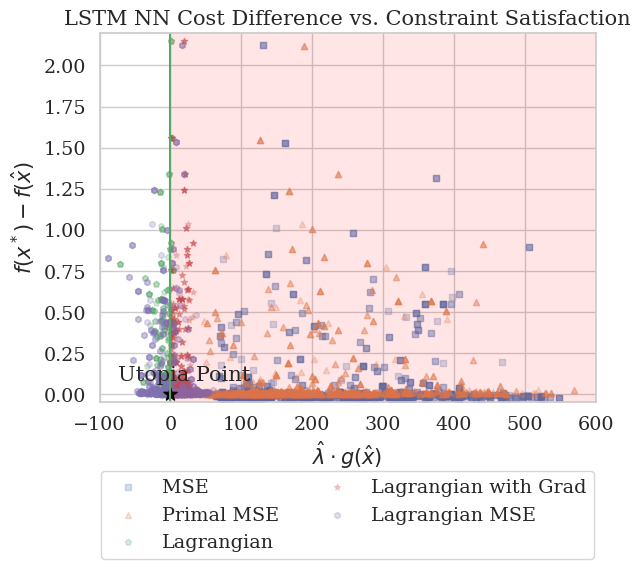
Figure 3: Cost difference vs. constraint satisfaction for TOAST LSTM predictions on test data.

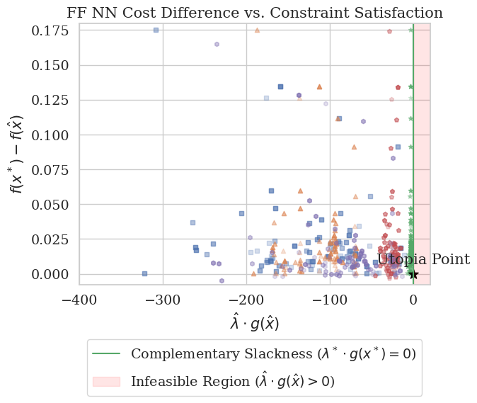
Figure 4: Cost difference vs. constraint satisfaction for TOAST feedforward predictions on test data.

We see immediately that, while close in cost prediction, primal MSE predictions are largely infeasible for the LSTM NN. Lagrangian loss-trained predictions demonstrate predictions which are the closest to meeting the complementary slackness condition, with Lagrangian with Grad and Lagrangian MSE close in constraint satisfaction.

Timing results from applying the LSTM and Feedforward trained NNs to the online inference problem are plotted in Figure 5. Overall, the Lagrangian-regularized MSE merit function and the Primal MSE are close in dominating performance. Lagrangian MSE has more than a 2 second improvement in mean computation time over MSE (4 vs. 6.22 seconds) for the Feedforward architecture and Primal MSE is just 190 ms less than the mean computation time for Lagrangian MSE for the LSTM architecture (2.78 vs. 2.97 seconds). When compared to the full SQP, all merit functions in the TOAST software architecture provide warm-starts which offer a significant reduction in computation time. With the decision-focused merit functions offering up to a 63% reduction in mean runtime for the LSTM NN and a 54% reduction in mean runtime for the Feedforward NN. Benchmarking against the MSE-based and collision-penalizing spacecraft swarm trajectory planning problem for 10 spacecraft, both warm start techniques reduce the 20 second mean solve time to less than 5 seconds (Sabol et al., 2022). While our implementation using 50 more timesteps and less than 8000 training samples has 2.97 and 4 second runtimes. Which we conclude are comparable with the mean warm-started runtimes provided by (Sabol et al., 2022).

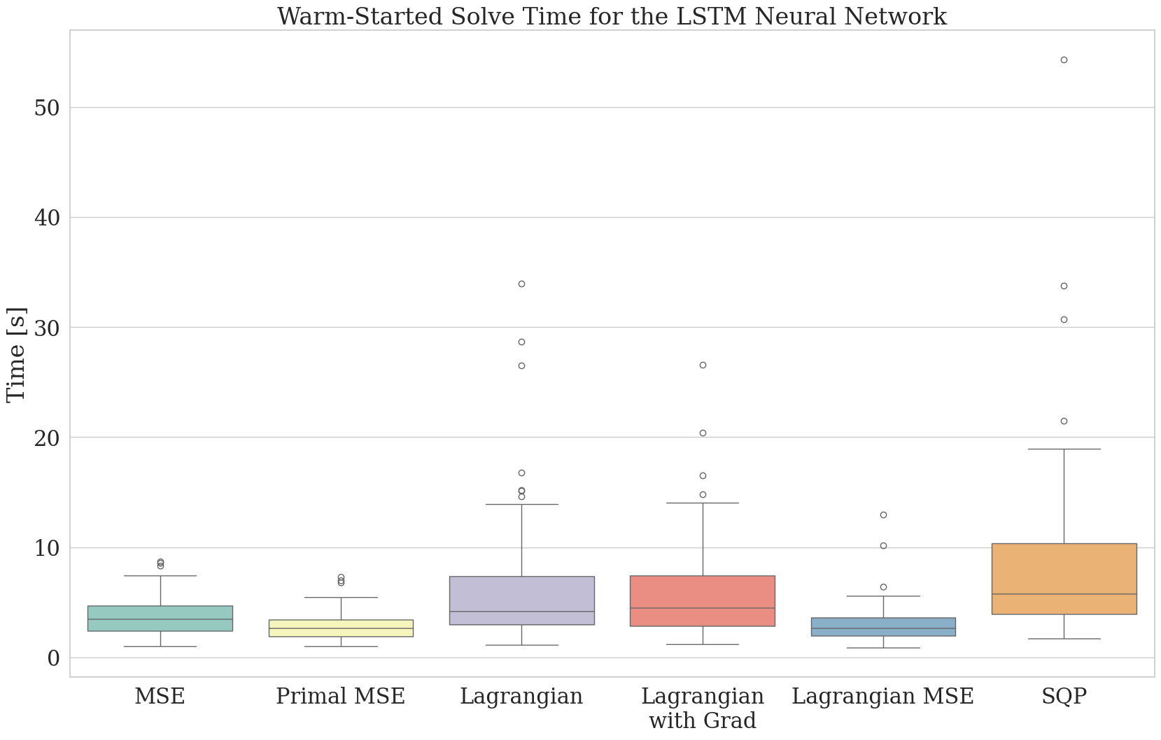
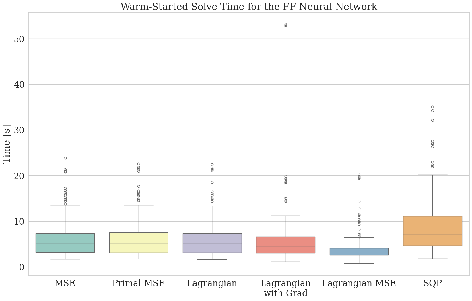
Figure 5: Computation time for test dataset warm-starts using TOAST. Both the LSTM NN and Feedforward NN provide more than a 5 second speedup from the SQP.

Table 1 shows the performance metrics for each loss function and the LSTM and Feedforward NN architectures, where CV is the percent of violated constraints, AD the average degree of constraint violation, and AD the mean $\pm$ the standard deviation. While the Feedforward NN denotes the Primal MSE loss as the merit function with the least state error, Lagrangian MSE achieves the minimum state error and Lagrangian with Grad achieves the minimum control error for the LSTM NN. These results show that with an LSTM architecture, regularizing the MSE loss term using the Lagrangian may improve decision variable prediction accuracy, in addition to constraint satisfaction. The Lagrangian with Grad NN achieves the least percent of violated constraints, $11.21\%$, as well as the smallest degree of violation, $8.59$, for the LSTM NN. For the Feedforward NN, Lagrangian MSE dominates in constraint satisfaction, achieving $1.21\%$ violated constraints and an $11.66$ degree of constraint violation, at the cost of a larger state error. Benchmarking against the NN architectures in (Sabol et al., 2022), the average number of collisions increase by 0.043-0.114 for the FF NNs and increase by 0.092 for one of the LSTM NNs when collision-penalization is applied. In contrast, TOAST reliably decreases constraint violation by $0.65\%-5.33\%$ for the LSTM NN and by $5.67\%-8.21\%$ for the Feedforward NN, when compared to vanilla MSE loss. Therefore, we have shown that decision-focused merit functions effectively learn trajectory predictions and feasibility.

Table 1: Performance Metrics for LSTM and FF Neural Networks

Architecture	Metric	LSTM	FF
MSE	CV (%) / AD	16.54 / 22.95 $\pm$ 2.12	9.42 / 17.95 $\pm$ 5.47
	MSE (State / Control)	3.53 / 0.032	0.157 / 0.00093
Primal MSE	CV (%) / AD	13.85 / 14.07 $\pm$ 5.98	12.56 / 15.73 $\pm$ 5.04
	MSE (State / Control)	0.068 / 0.033	0.122 / 0.005
Lagrangian	CV (%) / AD	15.89 / 11.00 $\pm$ 5.95	3.75 / 11.79 $\pm$ 3.42
	MSE (State / Control)	1.06 / 0.033	0.981 / 0.0035
Lagrangian w/ Grad	CV (%) / AD	11.21 / 8.59 $\pm$ 2.54	2.21 / 11.75 $\pm$ 3.48
	MSE (State / Control)	0.809 / 0.032	0.973 / 0.0008
Lagrangian MSE	CV (%) / AD	13.90 / 13.61 $\pm$ 5.95	1.21 / 11.66 $\pm$ 3.37
	MSE (State / Control)	0.068 / 0.032	1.01 / 0.00079

5 Conclusion

By employing a two-step process of offline supervision and online inference using decision-focused merit functions, TOAST computes a learned mapping biased towards constraint satisfaction. Three merit functions were designed for training: Lagrangian Loss, Lagrangian with Gradient Loss, and Lagrangian MSE Loss. After applying TOAST to learn the time-varying policy of lunar rover MPC, benchmarking results demonstrate the expected distributional shifts towards constraint satisfaction on test data and over a 5 second speedup. Future work will include new NN architectures, including a Transformer NN, and extend decision-focused learning to the problem of learning for nonconvex powered descent guidance trajectory generation.

6 Acknowledgments

The authors would like to thank Breanna Johnson and Dan Scharf for their discussions during the development of this work. This research was carried out at the Jet Propulsion Laboratory, California Institute of Technology, under a contract with the National Aeronautics and Space Administration and funded through the internal Research and Technology Development program. This work was supported in part by a NASA Space Technology Graduate Research Opportunity 80NSSC21K1301.

References

- Amos (2023) B. Amos. Tutorial on amortized optimization. Foundations and Trends in Machine Learning, 16(5):732, 2023.
- Andersson et al. (2019) J. A. E. Andersson, J. Gillis, G. Horn, J. B. Rawlings, and M. Diehl. CasADi: A software framework for nonlinear optimization and optimal control. Mathematical Programming Computation, 11(1):1–36, 2019.
- Betts (1998) J. T. Betts. Survey of numerical methods for trajectory optimization. AIAA Journal of Guidance, Control, and Dynamics, 21(2):193–207, 1998.
- Boyd and Vandenberghe (2004) S. Boyd and L. Vandenberghe. Convex Optimization. Cambridge Univ. Press, 2004.
- Briden et al. (2024) J. Briden, T. Gurga, B. Johnson, A. Cauligi, and R. Linares. Improving computational efficiency for powered descent guidance via transformer-based tight constraint prediction. In AIAA Scitech Forum, 2024.
- Cauligi et al. (2022a) A. Cauligi, A. Chakrabarty, S. Di Cairano, and R. Quirynen. PRISM: Recurrent neural networks and presolve methods for fast mixed-integer optimal control. In Learning for Dynamics & Control, 2022a.
- Cauligi et al. (2022b) A. Cauligi, P. Culbertson, E. Schmerling, M. Schwager, B. Stellato, and M. Pavone. CoCo: Online mixed-integer control via supervised learning. IEEE Robotics and Automation Letters, 7(2):1447–1454, 2022b.
- Chen et al. (2022) S. W. Chen, T. Wang, N. Atanasov, V. Kumar, and M. Morari. Large scale model predictive control with neural networks and primal active sets. Automatica, 135:109947, 2022.
- Dua et al. (2008) P. Dua, K. Kouramas, V. Dua, and E. N. Pistikopoulos. MPC on a chip - recent advances on the application of multi-parametric model-based control. Computers & Chemical Engineering, 32(4-5):754–765, 2008.
- Eren et al. (2017) U. Eren, A. Prach, B. B. Koçer, S. V. Raković, E. Kayacan, and B. Açikmese. Model predictive control in aerospace systems: Current state and opportunities. AIAA Journal of Guidance, Control, and Dynamics, 40(7):1541–1566, 2017.
- Haeser et al. (2021) G. Haeser, O. Hinder, and Y. Ye. On the behavior of Lagrange multipliers in convex and nonconvex infeasible interior point methods. Mathematical Programming, 186:257–288, 2021.
- Ichnowski et al. (2020) J. Ichnowski, Y. Avigal, V. Satish, and K. Goldberg. Deep learning can accelerate grasp-optimized motion planning. Science Robotics, 5(48):1–12, 2020.
- Keane et al. (2022) J. T. Keane, S. M. Tikoo, and J. Elliott. Endurance: Lunar South Pole-Atken Basin traverse and sample return rover. Technical report, National Academy Press, 2022.
- Kelly (2017) M. Kelly. An introduction to trajectory optimization: How to do your own direct collocation. SIAM Review, 59(4):849 – 904, 2017.
- Kingma and Ba (2015) D. P. Kingma and J. L. Ba. Adam: A method for stochastic optimization. In Int. Conf. on Learning Representations, 2015.
- Kotary et al. (2021) J. Kotary, F. Fioretto, P. Van Hentenryck, and B. Wilder. End-to-end constrained optimization learning: A survey. In Int. Joint Conf. on Artificial Intelligence, 2021.
- Liu et al. (2018) P. Liu, B. Paden, and U. Ozguner. Model predictive trajectory optimization and tracking for on-road autonomous vehicles. In Proc. IEEE Int. Conf. on Intelligent Transportation Systems, 2018.
- Mandi et al. (2023) J. Mandi, J. Kotary, S. Berden, M. Mulamba, V. Bucarey, T. Guns, and F. Fioretto. Decision-focused learning: Foundations, state of the art, benchmark and future opportunities, 2023. Available at https://arxiv.org/abs/2307.13565.
- National Academies of Sciences, Engineering, and Medicine (2022) National Academies of Sciences, Engineering, and Medicine. Origins, worlds, and life: A decadal strategy for planetary science and astrobiology 2023–2032. Technical report, National Academy Press, 2022.
- Nocedal and Wright (2006) J. Nocedal and S. J. Wright. Numerical Optimization. Springer, second edition, 2006.
- Paszke et al. (2017) A. Paszke, S. Gross, S. Chintala, G. Chanan, E. Yang, Z. DeVito, Z. Lin, A. Desmaison, L. Antiga, and A. Lerer. Automatic differentiation in PyTorch. In Conf. on Neural Information Processing Systems - Autodiff Workshop, 2017.
- Rankin et al. (2020) A. Rankin, M. Maimone, J. Biesiadecki, N. Patel, D. Levine, and O. Toupet. Driving Curiosity: Mars Rover mobility trends during the first seven years. In IEEE Aerospace Conference, 2020.
- Reske et al. (2021) A. Reske, J. Carius, Y. Ma, F. Farshidian, and M. Hutter. Imitation learning from MPC for quadrupedal multi-gait control. In Proc. IEEE Conf. on Robotics and Automation, 2021.
- Sabol et al. (2022) A. Sabol, K. Yun, M. Adil, C. Choi, and R. Madani. Machine learning based relative orbit transfer for swarm spacecraft motion planning. In IEEE Aerospace Conference, 2022.
- Sambharya et al. (2023) R. Sambharya, G. Hall, B. Amos, and B. Stellato. End-to-end learning to warm-start for real-time quadratic optimization. In Learning for Dynamics & Control, 2023.
- Szegedy et al. (2014) C. Szegedy, W. Zaremba, I. Sutskever, J. Bruna, D. Erhan, I. Goodfellow, and R. Fergus. Intriguing properties of neural networks, 2014. Available at https://arxiv.org/abs/1312.6199.
- Tagliabue et al. (2022) A. Tagliabue, D.-K. Kim, M. Everett, and J. P. How. Demonstration-efficient guided policy search via imitation of robust tube MPC. In Proc. IEEE Conf. on Robotics and Automation, 2022.
- Tang et al. (2018) G. Tang, W. Sun, and K. Hauser. Learning trajectories for real-time optimal control of quadrotors. In IEEE/RSJ Int. Conf. on Intelligent Robots & Systems, 2018.
- Verma et al. (2023) V. Verma, M. W. Maimone, D. M. Gaines, R. Francis, T. A. Estlin, S. R. Kuhn, G. R. Rabideau, S. A. Chien, M. McHenry, E. J. Graser, A. L. Rankin, and E. R. Thiel. Autonomous robotics is driving Perseverance rover’s progress on Mars. Science Robotics, 8(80):1–12, 2023.
- Wächter and Biegler (2006) A. Wächter and L. T. Biegler. On the implementation of an interior-point filter line-search algorithm for large-scale nonlinear programming. Mathematical Programming, 106(1):25–57, 2006.
- Wilder et al. (2019) B. Wilder, B. Dilkina, and M. Tambe. Melding the data-decisions pipeline: Decision-focused learning for combinatorial optimization. In Proc. AAAI Conf. on Artificial Intelligence, 2019.
- Zhang et al. (2019) X. Zhang, M. Bujarbaruah, and F. Borrelli. Safe and near-optimal policy learning for model predictive control using primal-dual neural networks. In American Control Conference, 2019.