Abstract

Generative Flow Networks (GFNs) have emerged as a powerful tool for sampling discrete objects from unnormalized distributions, offering a scalable alternative to Markov Chain Monte Carlo (MCMC) methods. While GFNs draw inspiration from maximum entropy reinforcement learning (RL), the connection between the two has largely been unclear and seemingly applicable only in specific cases. This paper addresses the connection by constructing an appropriate reward function, thereby establishing an exact relationship between GFNs and maximum entropy RL. This construction allows us to introduce maximum entropy GFNs, which, in contrast to GFNs with uniform backward policy, achieve the maximum entropy attainable by GFNs without constraints on the state space.

1 Introduction

Generative Flow Networks (GFNs) have recently emerged as a scalable method for sampling discrete objects from high-dimensional unnormalized distributions. They transform the complexity of navigating such spaces into a sequential decision-making problem, wherein each sequence of actions yields a unique object. Although the notion of framing "inference" as a control problem has been previously explored (Fleming and Mitter,, 1981; Buesing et al.,, 2020), Bengio et al., (2021) observe that a naive approach based on soft Q-learning (SQL; Haarnoja et al.,, 2017) and maximum entropy reinforcement learning (RL) tends to favor large objects disproportionately. To counter this, they introduced GFNs, a novel RL-inspired method.

While Bengio et al., (2021) established the exact equivalence between GFNs and SQL for tree-structured problems, GFNs have primarily been explored outside the theoretical confines of RL. This is due to the ambiguity over how this connection could be applicable more generally. Our work aims to bridge this knowledge gap by developing a valid GFN-like method purely from an RL standpoint. The crucial insight is that the sampling bias, identified by Bengio et al., (2021), can be mitigated by formulating a suitable reward function. Combined with the smooth Bellman equation, this leads to samples from the target distribution. We illustrate that this reward function can be efficiently obtained as the solution to an auxiliary dynamic programming problem, the number of paths leading to a specific node. Our resulting approaches, termed generative SQL, can further be interpreted as an instantiation of the concept of general value functions (Sutton et al.,, 2011; White,, 2015).

By leveraging our newly forged theoretical connection, we find the backward policy of a GFN whose forward policy corresponds to generative SQL, which we refer to as the maximum entropy backward and can be calculated using the same dynamic program used for generative SQL. We prove that maximum entropy GFNs, GFNs that use the maximum entropy backward, indeed achieve the upper bound of entropy possible for a GFN—a claim hinted at in prior research under stringent conditions (Zhang et al.,, 2022).

Additionally, we reveal that applying Path Consistent Learning (PCL; Nachum et al.,, 2017) on our proposed reward yields “trajectory-balance” for maximum entropy GFNs.

The principal contributions of this paper are as follows:

1. We propose a reward function with the property that, once incorporated within the smooth Bellman equations, leads to policies capable of sampling from the given target distribution.

2. We provide a formulation backward policy for GFNs with the same policy as the solution of the smooth Bellman equations.

3. We show that GFNs constructed in this manner have a unique solution- unlike traditional GFNs- and provably reach the maximum entropy in the general case.

4. We demonstrate through experiments that maximum entropy GFNs enhance the exploration of intermediate states and achieve better results in a hard graph-building environment.

2 Background and Notation

We provide a list of notation in Table LABEL:tab:notation and a list of abbreviations in Table LABEL:tab:abrev in the appendix.

A Markov decision process (MDP) is a tuple $(\mathcal{S},\mathcal{S}_{0},\mathcal{T},\mathcal{A},\mathds{A},T,\mathbb{P}_{0})$ where $\mathcal{S}$ is the set of states, $\mathcal{S}_{0}\subset\mathcal{S}$ is the set of initial states, and $\mathcal{T}\subset\mathcal{S}$ is the set of terminal states. Furthermore, $\mathcal{A}$ is the set of actions, the action mask $\mathds{A}:\mathcal{S}\rightarrow P(\mathcal{A})$, where $P$ is the power set function, is a function that defines the set of actions available at the state $s$, and $T:\mathcal{S}\times\mathcal{A}\rightarrow\mathcal{S}$ is the deterministic transition function that defines the next state given the current state and actions. The initial state of the trajectories is sampled from $\mathbb{P}_{0}:\Delta(\mathcal{S}_{0})$ where $\Delta(\mathcal{\mathcal{missing}}S_{0})$ denotes the set of all distributions over the set $\mathcal{S}_{0}$. We deviate the notation from that of Sutton and Barto, (2018) or Bengio et al., (2023) to both find a notation that helps us bridge the two topics and, at the same time, reflect the underlying assumptions and implementations better.

In the context of GFNs, Bengio et al., (2021) assume that there is a unique initial state $\mathcal{S}_{0}=\{s_{0}\}.$ Also central to the definition of GFNs is the parent function $\text{Parent}:\mathcal{S}\rightarrow P(\mathcal{S}\times\mathcal{A})$. It returns the set of state action pairs $(s,a)$ that reach a state $s^{\prime}$. It can be thought of as the generalized inverse of $T$ and is defined as

$$\text{Parent}(s^{\prime})=\{(s,a)\in\mathcal{S}\times\mathcal{A}|a\in\mathds{A}(s)\wedge T(s,a)=s^{\prime}\}.$$

Furthermore, GFNs assume that the transition function $T$ is acyclic (Bengio et al.,, 2021), which means it is impossible to reach a state from itself. We refer to MDPs with acyclic transition functions as acyclic MDPs for brevity. An essential consequence of the acyclicity assumption is that any regularized dynamic program (DP) converges and has a unique solution (Mensch and Blondel,, 2018).

For acyclic MDPs, we define the marginal state distribution $\mu_{\pi}:\mathcal{S}\rightarrow\mathbb{R}$ as the probability of passing through a state using the policy $\pi$. The marginal $\mu_{\pi}(s)$ can be calculated with dynamic programming for deterministic acyclic MDPs using the following recursion:

$$\mu_{\pi}(s^{\prime})=\sum_{\mathclap{(s,a)\in\text{Parent}(s^{\prime})}}\mu(s)\pi(a|s).$$

We note that $\mu(s)=\mathbb{P}_{0}(s)$ for all $s\in\mathcal{S}_{0}$ and $\sum_{s\in\mathcal{T}}\mu_{\pi}(s)=1$. We call a state “reachable” if there exists a sequence of actions leads to that state from a state in $\mathcal{S}_{0}$ whose initial probability $\mathbb{P}_{0}$ is greater than zero. If this property holds globally, we say that MDP is reachable.

Given an unnormalized distribution on the terminal states $\tilde{p}:\Delta(\mathcal{T})$ called the target, our goal is to find a policy $\pi:\mathcal{S}\rightarrow\Delta(\mathcal{A})$ such that the probability of reaching a terminal state $t\in\mathcal{T}$ is proportional to $\tilde{p}(t)$. For simplicity, we assume that $\tilde{p}$ is zero for all non-terminal states. We denote the normalized version of $\tilde{p}$ as $p$ and write the normalizing constant of the target or the partition function as $Z$.

2.1 Generative Flow Networks

GFNs enforce that for all terminal states $t\in\mathcal{T}$, the probability of ending the trajectory in $t$, i.e., $\mu(t)$, is proportional to $\tilde{p}$. In other words, the policy samples in proportion to $\tilde{p}$. They are built around the idea that the MDP is acyclic, i.e., no state can reach itself and that only one initial state $s_{0}$ exists. Concretely, any Markovian policy $\pi$ that samples terminal states in proportion to $\tilde{p}$ fits the detailed balance (DB) constraints

$$F(s)\pi(a|s)=q(s,a|s^{\prime})F(s^{\prime}),$$ (DB)

for all transition triplets $s^{\prime}=T(s,a)$, and where $q:\mathcal{S}\rightarrow\Delta(\mathcal{S}\times\mathcal{A})$ is the backward policy and $F:\mathcal{S}\rightarrow\mathbb{R}_{\geq 0}$ is the state flow function and is assumed to be equal to $\tilde{p}(t)$ for all terminal states $t\in\mathcal{T}$. The state flow and marginal are linked $F(s)/F(s_{0})=\mu(s)$. Any $\pi$ and $\tilde{p}$ uniquely identify the backward policy and the state flow function. Furthermore, for any $\pi$, $q$, and $F$ that fit (DB), $\pi$ samples in proportion to $\tilde{p}$ (Bengio et al.,, 2023).

Detailed balance (DB) is not the only formulation possible for a GFN; Trajectory Balance (TB; Malkin et al.,, 2022) is obtained by multiplying the (DB) constraint over a trajectory i.e.

$$Z\prod_{t=0}^{T-1}\pi(a_{t}|s_{t})=\tilde{p}(s_{T})\prod_{t=0}^{T-1}q(s_{t},a_{t}|s_{t+1}),$$ (TB)

where $Z$ is shorthand for $F(s_{0})$. Additional formulations for GFNs, including Bengio et al., (2021)’s original constraint, are included in Appendix LABEL:appen:gfn.

Bengio et al., (2021) propose minimizing the residual of a GFN constraint like (DB), which can admit an infinite number of solutions (see Appendix LABEL:appen:gfn). On the other hand, for any strictly concave function, there is only a unique GFN that maximizes that function. One example of a strictly concave function is the flow entropy, defined as

$$\mathbb{H}(\pi)=\mathbb{E}\left[\sum_{t=0}^{T-1}H(\pi(\cdot|s_{t}))\right]=\sum_{s\in\mathcal{S}}\mu_{\pi}(s)H(\pi(\cdot|s)),$$

where $H(\pi)=-\sum_{a\in\mathds{A}(s)}\pi(a|s)\log\pi(a|s)$ is the entropy. In Section 3.1, we not only show that flow entropy is strictly concave, we show it is equal to the entropy of the policy. Flow entropy was first introduced by Zhang et al., (2022) where they showed that for a restrictive class of MDPs setting the backward to be uniform on the parents (i.e., $q(s,a|s^{\prime})=1/|\text{Parent}(s^{\prime})|$) maximizes the flow entropy. However, Zhang et al., (2022) restrict the class of MDPs they analyze so much as to exclude the drug design MDP of Bengio et al., (2021). Concretely, Zhang et al., (2022) look at MDPs where the state is a vector of values and placeholders, and each action sets a placeholder to a value. For instance, the state could be $(\star,\star,0)$, for the placeholder $\star$, and the action “set element $0$ to $1$” would yield the state $(1,\star,0)$. While many MDPs used on GFNs add elements to placeholders, this definition is much more restrictive. Zhang et al., (2022)’s construction can be relaxed to having MDPs with finite and fixed horizons where the transition function is layered, meaning that there exists a partitioning of the state space $\mathcal{L}_{0},\mathcal{L}_{1},\mathcal{L}_{2},\ldots,\mathcal{L}_{n}$ where $\mathcal{L}_{0}=\mathcal{S}_{0}$, $\mathcal{L}_{n}=\mathcal{T}$ and the parents of any set in layer $\mathcal{L}_{i}$ is in $\mathcal{L}_{i-1}$ for $i\geq 1$. Furthermore, they assume that the number of actions in layer $\mathcal{L}_{i}$ is $n-i$. These assumptions are restrictive; for instance, adding the constraint that the number of ones is always less than the number of zeros invalidates the assumptions.

2.2 Soft Q-learning

Given a reward function over transitions $R:\mathcal{S}\times\mathcal{A}\rightarrow\mathbb{R}$, terminal reward $R_{\mathcal{T}}:\mathcal{T}\rightarrow\mathbb{R}$, along with the discount factor $\gamma\in(0,1]$, we can derive two fundamental functions: the state value function $V(s)$, and the state-action value function $Q(s,a)$. The state value function $V(s)$ represents the maximum discounted reward obtainable from the state $s$, while the state-action value function $Q(s,a)$ represents the maximum discounted reward from state $s$ when taking the action $a$. The Bellman equation (Bellman,, 1954) articulates the relationship between the $V$ and $Q$ functions. This equation can be formulated as:

$$Q(s,a) =R(s,a)+\gamma V(T(s,a)),$$ (1a)

$$V(s) =\max_{a\in\mathds{A}(s)}Q(s,a).$$ (1b)

We assume that the value of the V function is the terminal reward at the terminal states, i.e., $V(t)=R_{\mathcal{T}}(t)$ for all $t\in\mathcal{T}$.

If we augment the reward with the entropy or an i.i.d. Gumbel term to the maximum in (1b), we obtain the soft (smooth) Bellman equation (Rust,, 1987; Todorov,, 2006; Ziebart et al.,, 2008; Peters et al.,, 2010; Rawlik et al.,, 2012; Fosgerau et al.,, 2013; Van Hoof et al.,, 2015; Fox et al.,, 2016; Nachum et al.,, 2017; Haarnoja et al.,, 2017; Geist et al.,, 2019; Garg et al.,, 2023)

$$Q(s,a) =R(s,a)+\gamma V(T(s,a))$$ (2a)

$$V(s) =\max_{\pi\in\Delta(\mathds{A}(s))}\mathbb{E}_{a\sim\pi}[Q(s,a)-\tau\log\pi_{a}],$$ (2b)

at temperature $\tau$. If $\gamma$ is less than one, the soft Bellman equation will have a unique solution (Geist et al.,, 2019). However, the existence of a unique solution is not guaranteed in the undiscounted case, i.e., where $\gamma=1$. Mai and Frejinger, (2022, Remark 2) give a sufficient condition for the existence of a unique solution. In the acyclic case, Mensch and Blondel, (2018) showed that the soft Bellman equation has a unique solution. We note that there cannot be more than one solution to the equations as entropy is strictly concave.

Given a Q function, the value function $V$ is equal to $V(s)=\tau\log\sum_{a\in\mathds{A}(s)}\exp(Q(s,a)/\tau),$ and the policy is $\pi(a|s)=\frac{\exp(Q(s,a)/\tau)}{\sum_{a^{\prime}\in\mathds{A}(s)}\exp\left(Q(s,a^{\prime})/\tau\right)}=\exp\left(Q(s,a)/\tau-V(s)/\tau\right).$ Taking the log on both sides of this expression is the basis for Path consistency learning (PCL) (Nachum et al.,, 2017), which aims to enforce a temporal consistency between the policy and value function over multiple steps. For deterministic MDPs, Path Consistency Learning enforces

$$V(s_{i})+\sum_{t=i}^{j-1}\tau\gamma^{t-i}(\tau\log\pi(a_{t}|s_{t})-R(s_{t},a_{t}))\\ =\gamma^{j-i}V(s_{j})$$ (3)

instead of the soft Bellman equation over a sub trajectory ${s}_{i},\allowbreak{a}_{i},\allowbreak\ldots,\allowbreak{s}_{j-1},\allowbreak{a}_{j-1},\allowbreak{s}_{j}$. We note that the relationship between (TB) and (DB) is reminiscent of (3) and (2).

In the remainder of this paper, we assume $\tau=1$ and $\gamma=1$ for clarity unless explicitly stated.

A key property we use in our proofs is that the probability of a trajectory can be determined using the value function of its starting and ending states, along with the rewards accrued throughout that trajectory. This is further demonstrated in the following proposition.

Proposition 1.

(Fosgerau et al.,, 2013) in deterministic entropy regularized MDPs with no discounting we have $\log\mathbb{P}({s}_{i},\allowbreak{a}_{i},\allowbreak\ldots,\allowbreak{s}_{j-1},\allowbreak{a}_{j-1},\allowbreak{s}_{j})=\sum_{t=i}^{j-1}\log\pi(a_{t}|s_{t})=V(s_{j})+\sum_{t=i}^{j-1}R(s_{t},a_{t})-V(s_{i})$.

By Proposition 1, the likelihood of trajectories that share initial and terminal states is proportional to the exponent of their reward difference. If there are no intermediate rewards, they have the same probability. This property is important for our proofs.

3 From Soft Q-Learning to Maximum entropy Generative flow networks

In this section, we derive a policy that reaches terminal states in proportion to an unnormalized distribution $\tilde{p}$ by constructing an appropriate reward under the soft Bellman equations. As a reminder, we assume an acyclic deterministic MDP with only one initial state. The acyclicity assumption reflects that we are building complex discrete objects by accumulation of primitive parts. As for the assumption of a single initial state, it simply reflects the fact that we start over every time. These assumptions mirror the assumptions of GFNs. All proofs are in the appendix.

If we set $R(s,a)=0$ and $R_{\mathcal{T}}(s_{T})=\tilde{p}(s_{T})$, the return for a trajectory ${s}_{0},\allowbreak{a}_{0},\allowbreak\ldots,\allowbreak{s}_{T-1},\allowbreak{a}_{T-1},\allowbreak{s}_{T}$ is $\tilde{p}(s_{T})$. By Proposition 1, the likelihood of taking the trajectory is proportional to $\exp\tilde{p}(s_{T})$. Thus, we can estimate the probability of sampling any terminal state, given the number of trajectories that lead to that state.

Proposition 2.

[Proposition 1 in][]bengio2021flow For a terminal state $t\in\mathcal{T}$ and the numer of trajectories starting at $s_{0}$ that terminate in $t$, $n(t)$, the probability of a trajectory terminating in $t$, if we set the terminal reward $R_{\mathcal{T}}(t)$ to $\tilde{p}(t)$ and have no intermediate reward, is proportional to $n(t)\exp(\tilde{p}(t))$.

We include the proof since it is more concise than the one in Bengio et al., (2021). In the next proposition, we modify our reward function such that SQL samples terminal states in proportion to $\tilde{p}$.

Proposition 3.

For terminal reward $R_{\mathcal{T}}(t)=\log\tilde{p}(t)-\log n(t)$, the probability of reaching the state $t$ is proportional to $\tilde{p}(t)$.

Definition 1.

We call soft Q-Learning with the rewards $R(s,a)=0$ and terminal rewards $R_{\mathcal{T}}(s)=\log\tilde{p}(s)-\log n(s)$ generative soft Q-learning or GSQL.

In Appendix LABEL:appen:n we show that it is possible to calculate $n(s)$ for certain MDPs with combinatorial structures but in general $n(s)$ can be calculated using DP.

Theorem 1.

The number of trajectories $n(s)$ satisfies

$$n(s)=\sum_{(s^{\prime},a^{\prime})\in\text{Parent}(s)}n(s^{\prime}),$$ (4)

and $n(s_{0})=1$.

For most MDPs, the recursion of Theorem 1 is not tractable as the size of the DP table grows exponentially with respect to the horizon. Instead, we advocate learning $n$. Using the inverted MDP defined below, we show that we can leverage entropy regularized RL methods to learn $n$.

Definition 2.

The inverse of an MDP

$$(\mathcal{S},\mathcal{S}_{0},\mathcal{T},\mathcal{A},\mathds{A},T)$$

is an MDP

$$(\mathcal{S},\mathcal{T},\mathcal{S}_{0},\mathcal{S}\times\mathcal{A},\text{Parent},\bar{T})$$

where the set of actions is the set of state action pairs of the original MDP, the action mask function is the set of parents, and the inverted dynamics $\bar{T}$ undoes the action such that $\bar{T}(s^{\prime},(s,a))=s$. We omit $\mathbb{P}_{0}$ because it does not affect the calculations.

Note that the inverse MDP is implicitly present in the definition of GFNs as the backward policy is defined on the inverted MDP and that the inverse of the inverted MDP is the original MDP. Every trajectory ${s}_{0},\allowbreak{a}_{0},\allowbreak\ldots,\allowbreak{s}_{T-1},\allowbreak{a}_{T-1},\allowbreak{s}_{T}$ in the original MDP has a corresponding trajectory $s_{T},(s_{T-1},a_{T-1}),s_{T-1},\ldots,(s_{0},a_{0}),s_{0}$ in the inverted MDP. Using the inverted MDP, the dependence of $n(s)$ on the parents becomes a dependence on the children, giving rise to a formulation that uses a Bellman equation.

It is convenient to learn $\log n$ both for numerical purposes and for the synergy it has with Soft Q-learning. In the log space, the sum in (4) is replaced by a log-sum-exp. Indeed, as the following proposition shows, $\log n$, denoted as $l$, fits the soft Bellman equation.

Proposition 4.

Let $l(s)=\log n(s)$, then $l$ is the value function of the soft Bellman equation in the inverted MDP with the rewards set to zero for all states and transitions.

Figure 1: Comparison of maximum entropy and uniform backward. Left: uniform backward policy, middle: MDP, right: maximum entropy gflownet. The numbers are the probabilities of the policies at state $s_{0}$ and $s_{2}$.

Proposition 4 allow us to use standard entropy regularized RL tools to learn $n$. This allows us to assert that learning $n$ is not harder than learning the GFN. Indeed, as shown in the experiment section, it is often easier. Any constraint like the soft Bellman equation and PCL can be used. If PCL is used, let $\log q((s,a)|s^{\prime})=l(s)-l(s^{\prime})$, the PCL equation becomes $l(s_{j})+\sum_{t=i}^{j-1}\log q((s_{t},a_{t})|s_{t+1})=l(s_{i})$. We revisit this $q$ in Section 3.2. Notice how the value of the initial state in the trajectories is on the right-hand side, not the left-hand side, as we are using a consistency equation on the inverted MDP.

The next proposition shows that the value initial state $s_{0}$ of GSQL equals the logarithm of total flow $\log F(s_{0})$ or $\log Z$. We begin with a lemma that shows that the value of every state $s$ is the log-sum-exp of all trajectories that pass through $s$. Using trajectories instead of terminal states allows us to not run into issues when a state is the descendent of multiple states that are not the descent of each other.

Lemma 1.

In finite acyclic MDPs with $R(s,a)=0$, $V(s)$ is equal to the log-sum-exp of the reward of all trajectories that start at $s$.

Equipped with Lemma 1, we can show the following proposition for GSQL.

Proposition 5.

The value function of the initial state is equal to the logarithm of the partition function, i.e., $V(s_{0})=\log\sum_{s\in\mathcal{T}}\tilde{p}(s)=\log Z$.

3.1 A different definition of flow entropy

This subsection shows that flow entropy equals entropy over trajectories and that GSQL achieves maximum entropy. We define the trajectory entropy as follows:

Definition 3.

The trajectory entropy $H$ is the entropy over a set of trajectories and is defined as

$$H(\pi)=\mathbb{E}\left[\sum_{t=0}^{T-1}\log\pi(a_{t}|s_{t})\right]$$ (5)

for Markovian policies.

The definition is trivially extendable to non-Markovian policies as it is the entropy of the distribution over trajectories. The following proposition shows that $\mathbb{H}$ and $H$ are, in fact, equal.

Proposition 6.

The trajectory entropy and flow entropy are equal for Markovian policies, i.e., $\mathbb{H}(\pi)=H(\pi)$.

Theorem 2.

GSQL achieves the maximum entropy a policy sampling in proportion to the target can achieve.

The uniqueness of the maximum entropy GFN is derived from the following concavity proof.

Proposition 7.

Markovian entropy is strictly concave and thus the maximum entropy GFN is unique.

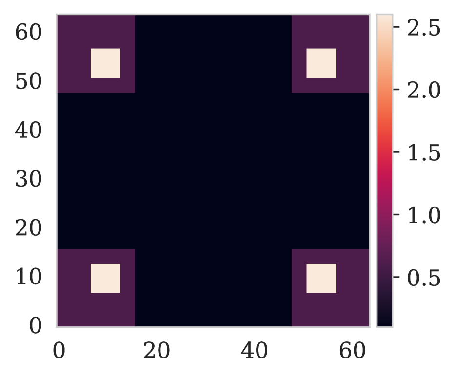
(a) $\tilde{p}$

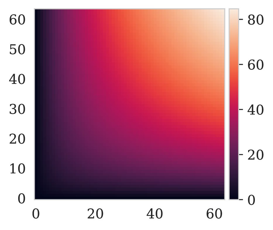
(b) $l$

(c) uniform $\mu$

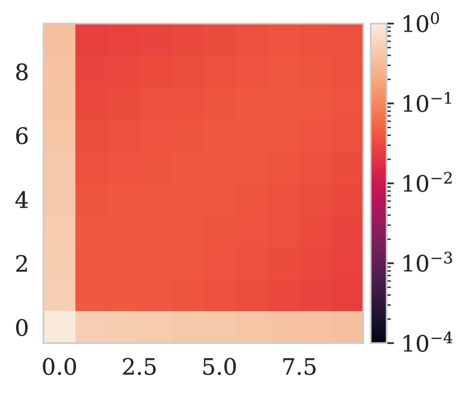
(d) uniform $\mu$ zoomed

(e) maxent $\mu$

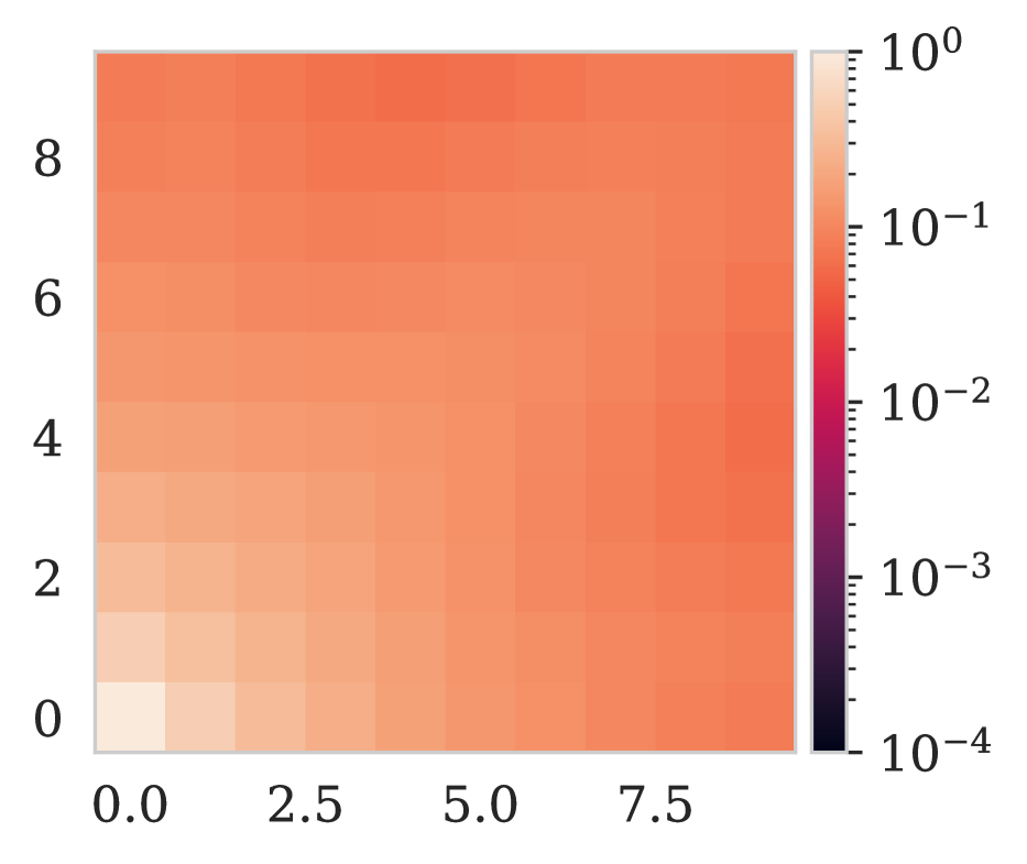
(f) maxent $\mu$ zoomed

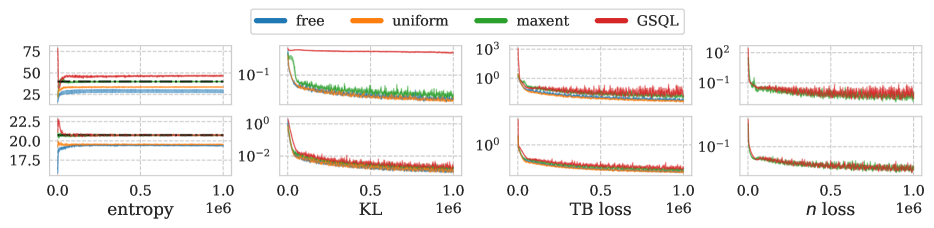
Figure 2: From left to right, target, $l$, and marginal of the uniform backward and maximum entropy GFNs for the $64^{2}$ grid. Note the log scale colors for $\mu$ and the non-smooth partitioning of the flow around the bottom and left edges with the uniform backward policy.

Figure 3: Various metrics for the hypergrid experiments. The top row is for the $64^{2}$ grid and the bottom row is for the $8^{4}$ grid. The black line shows the maximum entropy which is attained by both maxent and GSQL in the $8^{4}$ grid. Note the log y-scale for plots other than entropy.

3.2 The backward of GSQL

As mentioned in the introduction, for a fixed policy and $\tilde{p}$, we can uniquely identify the backward policy $q$. The following identifies the backward policy of GSQL.

Theorem 3.

The backward policy $q$ of the policy of GSQL is

$$q(s,a|s^{\prime})=n(s)/n(s^{\prime}).$$ (6)

The backward proposed here can be used to train maximum entropy GFNs.

Remark 1.

The backward policy $q$ gives a uniform distribution over all backward trajectories leading to $s_{0}$, given $s_{T}\in\mathcal{T}$.

Remark 2.

For a sub trajectory ${s}_{i},\allowbreak{a}_{i},\allowbreak\ldots,\allowbreak{s}_{j-1},\allowbreak{a}_{j-1},\allowbreak{s}_{j}$, $\prod_{t=i}^{j-1}q(s_{t},a_{t}|s_{t+1})=n(s_{i})/n(s_{j})$.

Remark 3.

We find the uniform backward if the number of paths to all parent nodes is equal. This can happen if the MDP is layered and the number of parents is the same for all nodes in all layers. Thus, the maximum entropy backward subsumes the uniform backward.

Note that the uniform backward is not always maximum entropy. For instance, as shown in Appendix LABEL:appen:n, it is not for any of the MDPs we analyze.

One major difference between GSQL and maximum entropy GFNs is what happens if $n$ is not learned to high fidelity. If $n(s)$ is greater than zero, then maximum entropy GFNs will still be GFNs yet GSQL does not have this property.

Lastly, unlike the uniform backward policy, the maximum entropy backward relaxes the reachability assumption. This is because $n$ is zero for unreachable states. However, this may require sampling backward trajectories similar to Zhang et al., (2022), which is beyond the scope of this work.

3.3 Remarks on PCL

Nachum et al., (2017) showed that if (3) holds for all sub-trajectories of a certain length, then the soft Bellman equation holds and vice versa. We extend the result to full trajectories.

Proposition 8.

If PCL holds for all sub-trajectories reaching a terminal state (${s}_{i},\allowbreak{a}_{i},\allowbreak\ldots,\allowbreak{s}_{T-1},\allowbreak{a}_{T-1},\allowbreak{s}_{T}$), all trajectories starting at an initial state (${s}_{0},\allowbreak{a}_{0},\allowbreak\ldots,\allowbreak{s}_{i-1},\allowbreak{a}_{i-1},\allowbreak{s}_{i}$), or all full trajectories (${s}_{0},\allowbreak{a}_{0},\allowbreak\ldots,\allowbreak{s}_{T-1},\allowbreak{a}_{T-1},\allowbreak{s}_{T}$), then it holds for all sub-trajectories. We call these conditions the terminal, initial, and trajectory PCL conditions, respectively.

We can use PCL to calculate $n$ using Proposition 4.

Proposition 9.

Given $n$, maximum entropy GFNs with (TB) and GSQL with trajectory 3 have the same residual and gradient.

4 Experiments

This section is divided into three subsections, each focusing on MDPs that do not follow the assumptions of Zhang et al., (2022). They help illustrate that it is not hard to find MDPs where the uniform backward is not maximum entropy. We compare maximum entropy GFNs and GSQL with GFNs with uniform and learned backward policies.

Appendix LABEL:appen:exp presents all experiment details, pseudocode, and further experiments.

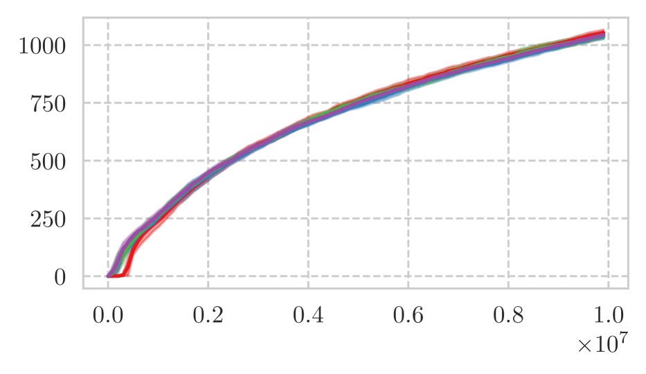
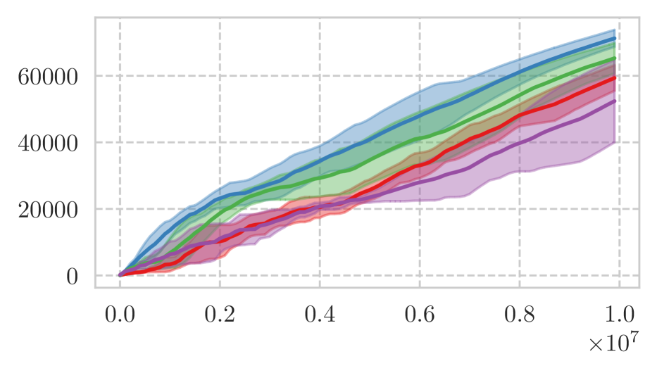
(a) number of modes found

(b) policy loss

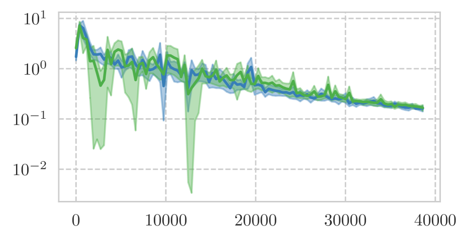
(c) $n$ loss

Figure 4: Experiment statistics. Confidence intervals show the IQM. From top to bottom, the rows belong to the sEH and QM9 experiments.

4.1 A simple MDP

In the MDP presented in Figure 1, there are three paths from the initial state $s_{0}$ to the destination $s_{T}$: $s_{0},s_{1},s_{T}$, $s_{0},s_{2},s_{1},s_{T}$, and $s_{0},s_{2},s_{T}$. The uniform backward gives $q(s_{1}|s_{T})=q(s_{2}|s_{T})=q(s_{0}|s_{1})=q(s_{2}|s_{1})=1/2$; thus, the paths have probabilities 0.25, 0.25, and 0.5, respectively, yielding an entropy of $3/2\log 2$. The maximum entropy GFN yields the backward $q(s_{1}|s_{T})=2/3$ and $q(s_{2}|s_{T})=1/3$ since there are 2 paths from $s_{1}$ but only one path from $s_{2}$. Furthermore, $q(s_{2}|s_{1})=q(s_{0}|s_{1})=1/2$, since only one path per parent exists. The entropy is $\log 3$, which is the maximum entropy.

4.2 Hypergrid

We now focus on the hypergrid domain from Bengio et al., (2021). The state is a vector that starts at $0$. At each step, the agent can increase one of the components of the vector by one, i.e., move one step in one of the directions or terminate the episode. The agent is in a bounded box, and the target function is given by

for the indicator function $\mathbb{I}$ and the ratio of the current position and the maximum allowed position in component $i$, $s_{i}$. In Figure 3, for a $64\times 64$ grid, we show the target, the logarithm of the number of paths $l$, and the marginal distribution of uniform backward policy and the maximum entropy GFNs. First, note that $l$ gets very big. We cannot store $n=\exp(l)$ as a 64-bit integer as $n$ for the top right corner is $(2\times 63)!/63!/63!$. Second, notice how the maximum entropy GFN distributes the flow more evenly and does not accumulate flow on the bottom and left edges.

We test the models on the $64^{2}$ and $8^{4}$ hypergrids to reach terminal states in proportion to (7). The results can be seen in Figure 3. In the $64^{2}$ experiments, GSQL failed to reach all modes but worked fine on the $8^{4}$ grid, whereas maximum entropy GFN successfully learns to sample in proportion to the target. The failure of GSQL is minor as it can be alleviated with added exploration, yet it illustrates the difference between GSQL and maximum entropy GFNs. Indeed, maximum entropy GFNs, unlike GSQL, are GFNs regardless of the quality of the estimated $n$. We note that since GSQL fails to learn the target distribution in the $64^{2}$ experiment, the fact that its entropy is higher than the maximum entropy is irrelevant.

Table 1: KL divergence of the policy of different models on small sEH task of Shen et al., (2023). The cells show the average KL divergence between the row and column policies.

		free	uniform	maxent		GSQL
	$n$			known	learned	known	learned
free		$0.32$ p m 0.06	$12.61$ p m 0.23	$11.03$ p m 0.23	$11.27$ p m 0.23	$11.13$ p m 0.23	$11.29$ p m 0.22
uniform		$10.69$ p m 0.37	$0.08$ p m 0.01	$0.38$ p m 0.01	$0.41$ p m 0.01	$0.39$ p m 0.01	$0.40$ p m 0.02
maxent	known	$10.02$ p m 0.37	$0.45$ p m 0.01	$0.05$ p m 0.01	$0.09$ p m 0.01	$0.08$ p m 0.01	$0.10$ p m 0.01
	learned	$9.83$ p m 0.36	$0.53$ p m 0.03	$0.09$ p m 0.01	$0.05$ p m 0.01	$0.10$ p m 0.01	$0.07$ p m 0.01
GSQL	known	$10.22$ p m 0.37	$0.56$ p m 0.02	$0.10$ p m 0.01	$0.12$ p m 0.01	$0.09$ p m 0.01	$0.12$ p m 0.01
	learned	$9.94$ p m 0.37	$0.52$ p m 0.01	$0.11$ p m 0.01	$0.09$ p m 0.01	$0.11$ p m 0.01	$0.08$ p m 0.01

4.3 Molecule design

In this section, we examine the sEH task of Bengio et al., (2021) and the QM9 task of Jain et al., (2023). We use a tree-building MDP in the sEH (Jin et al.,, 2018) and a graph-building MDP in the QM9 experiments. In the tree-building environment, every state is a tree, and each action either adds a node and connects it to an existing node or sets an attribute on each edge. In the sEH experiments, each node represents a fragment (collection of atoms), and edge features show the place of connection of two fragments. In the graph-building environment, every state is a connected graph (every node is reachable from every other node), and actions either add a new node and edge or set the attribute on edge.

The graph-building environment is more expressive than the tree-building environment. However, unlike the tree-building environment, the graph-building environment can lead to molecules that cannot exist and are invalid.

The tree-building MDP is much more structured, and we can calculate $n$ for each state directly to verify that we are, in fact, learning (see Appendix LABEL:appen:n). Figure 5 shows the mean squared error between the predicted $\log n$ and the real $\log n$. The difference between the learned $n$ and the ground truth is small.

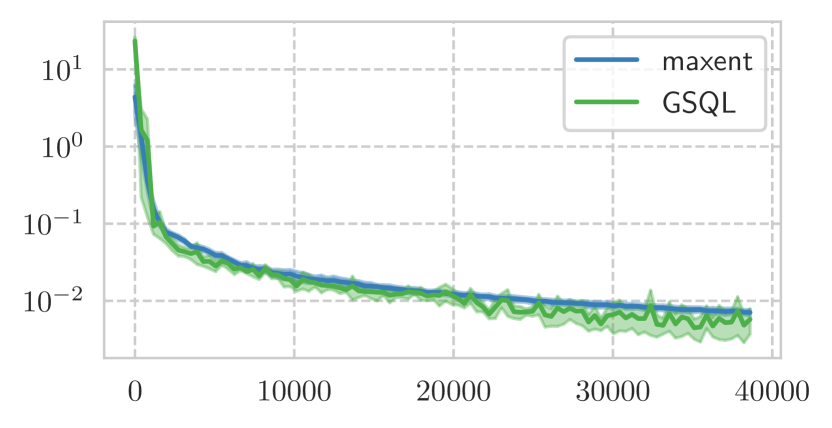
Figure 5: MSE of the learned $n$ and the ground truth in the sEH experiments.

We show the KL divergence between the policies found using different methods in Table 1 when trained using the small sEH MDP of Shen et al., (2023). Notice how GFNs with free backward policy have a higher KL divergence among themselves than the other policies. Indeed, this results from the GFN constraints having infinite feasible solutions for this MDP. As expected, GSQL and maximum entropy GFNs find close policies. We also note that they are close regardless of whether $n$ is given or learned. Lastly, as shown by the higher KL divergence between the GFNs with uniform backward policy and maximum entropy GFNs, the other two find different policies.

Next, we focus on the full sEH task; we show the GFN and $n$ losses in the top row of Figure 4(b) and Figure 4(c). Not only $n$ is learnable, but it is also is easier to learn than the policy constraint as the reward is always zero. As shown in the top row of Figure 4(a), GFNs with free backward policy start finding modes with a short lag. We show some statistics after training in Table 2. The top $K$ statistics are the same for all policies thus we can infer that all models are GFNs regardless of the backward but not using a free backward policy helps at the initial phase of the training and using maximum entropy backward policy policy increases the entropy. We refer to Appendix LABEL:appen:exp for a definition of the top $K$ statistics.

Our last set of experiments focuses on the QM9 experiments. While we calculated $n$ for the sEH experiments, we do not do so here as it is prohibitively expensive to do via the general recursion, and we could not find a combinatorial structure to exploit. As shown in the second row of Figure 4(b) and Figure 4(c), it is harder than the sEH experiment, but the $n$ objective is still easier than the policy objective. The bottom row of Figure 4(a) shows that maxent GFNs outperform GSQL, and GSQL outperforms the other two GFNs. Table 3 shows some statistics. We note that we put a hard limit of 100,000 modes as the cost of finding modes grows quadratically. In this experiment, maxent GFN and GSQL backward find more modes. Again, the key takeaway is that as we deviate more from the assumptions of Zhang et al., (2022), the performance of GFNs with uniform backward worsen.

Table 2: sEH experiment results.

model	$n$	entropy	diverse top $K$ reward	top $K$ diversity	top $K$ reward	modes with $\tilde{p}\geq 1$	modes with $\tilde{p}\geq 0.875$
free	none	$77.92$ p m 0.02	$1.03$ p m 0.00	$0.46$ p m 0.00	$1.03$ p m 0.00	$1049.90$ p m 5.66	$3378.00$ p m 24.30
uniform	none	$77.27$ p m 0.02	$1.03$ p m 0.00	$0.46$ p m 0.00	$1.03$ p m 0.00	$1042.90$ p m 5.21	$3318.30$ p m 31.15
GSQL	learned	$78.42$ p m 0.02	$1.03$ p m 0.00	$0.46$ p m 0.00	$1.03$ p m 0.00	$1043.90$ p m 7.18	$3446.50$ p m 40.27
	known	$78.39$ p m 0.01	$1.03$ p m 0.00	$0.46$ p m 0.00	$1.03$ p m 0.00	$1036.60$ p m 7.74	$3379.90$ p m 29.55
maxent	learned	$78.41$ p m 0.03	$1.03$ p m 0.00	$0.46$ p m 0.00	$1.03$ p m 0.00	$1035.70$ p m 5.56	$3417.60$ p m 32.82
	known	$78.41$ p m 0.02	$1.03$ p m 0.00	$0.46$ p m 0.00	$1.03$ p m 0.00	$1042.50$ p m 5.98	$3344.00$ p m 44.67

Table 3: QM9 experiment results.

model	entropy	diverse top $K$ reward	top $K$ diversity	top k reward	modes with $\tilde{p}\geq 1.125$	modes with $\tilde{p}\geq 1$
free	$93.41$ p m 0.24	$1.20$ p m 0.00	$0.83$ p m 0.00	$1.20$ p m 0.00	$60\,465$ p m 2157	$100\,000$ p m 0
uniform	$89.96$ p m 7.61	$1.19$ p m 0.01	$0.81$ p m 0.04	$1.19$ p m 0.01	$52\,865$ p m 4481	$100\,000$ p m 0
GSQL	$98.59$ p m 0.30	$1.19$ p m 0.00	$0.84$ p m 0.00	$1.19$ p m 0.00	$63\,909$ p m 2730	$100\,000$ p m 0
maxent	$98.22$ p m 0.11	$1.20$ p m 0.00	$0.83$ p m 0.00	$1.20$ p m 0.00	$71\,339$ p m 1468	$100\,000$ p m 0

5 Conclusion

This work showed an equivalence between entropy-regularized RL and GFNs. Concretely, we showed that using the number of trajectories to each terminal state, we can create a reward such that the probability of reaching terminal states of entropy-regularized RL is proportional to an unnormalized distribution. We use the equivalence to show the equivalence of (TB) and (3) for a specific class GFNs and entropy regularized RL with our proposed reward.

Building on top of our proposed extension of entropy regularized RL, we introduced maximum entropy GFNs, subsuming the uniform backward policy of Zhang et al., (2022). A benefit of our model is that it automatically falls back to the uniform backward policy whenever the uniform backward policy is maximum entropy. We showed that we can learn $n$ using the soft Bellman equation on the inverted MDP, as calculating it via the recursion may be too expensive, and a combinatorial structure may be hard to identify, as is the case with the graph-building environment used in the QM9 experiments. We then verified that $n$ is indeed learnable empirically.

While we mirror the assumptions of Bengio et al., (2021), our analysis is limited to undiscounted MDPs with deterministic transitions and only one initial state. Solving the same problem with stochastic transitions may be of interest (e.g. Pan et al.,, 2023) but is more complex. For instance, while the reachability of the terminal states guarantees a solution in the deterministic case, a solution may not exist in the stochastic formulation of Pan et al., (2023). Jiralerspong et al., (2023)’s formulation for GFNs in stochastic MDPs overcome the feasibility issue of Pan et al., (2023)’s formulation and maximum entropy GFNs may help relax the tree assumption of Jiralerspong et al., (2023) yet maintain their equilibrium results. However, it is unclear how to define the corresponding inverse MDP properly.

With our equivalence results, many RL algorithm like Munchausen Vieillard et al., (2020) are now directly applicable to GFNs. Future work will look at the improvements those methods can bring.

Derman et al., (2021) pointed out that entropy-regularized RL is equivalent to a particular robust reinforcement learning formulation. However, it is unclear how such a result would apply meaningfully here as the uncertainty set that Derman et al., (2021) proposes would give non-zero reward to transitions, something we cannot have with GFNs.

Current GFN environments are too structured. Most non-toy environments have many of the features Zhang et al., (2022) require. For instance, the MDPs we analyze are all layered but do not have the same number of parents. In the sEH experiment, the bulk of the high-reward molecules are in the final layer. We expect as the MDPs used become more and more complex, maximum entropy GFNs shine more as they did in QM9 experiment compared to the sEH experiment.

Acknowledgments

We thank Nikolay Malkin for helpful discussions around uniform backward GFNs. This research was supported by compute resources provided by Calcul Quebec (calculquebec.ca), the BC DRI Group, the Digital Research Alliance of Canada (alliancecan.ca), and Mila (mila.quebec).

References

- Bellman, (1954) Bellman, R. (1954). The theory of dynamic programming. Bulletin of the American Mathematical Society, 60(6):503–515.
- Bengio et al., (2021) Bengio, E., Jain, M., Korablyov, M., Precup, D., and Bengio, Y. (2021). Flow network based generative models for non-iterative diverse candidate generation. Advances in Neural Information Processing Systems, 34:27381–27394.
- Bengio et al., (2023) Bengio, Y., Lahlou, S., Deleu, T., Hu, E. J., Tiwari, M., and Bengio, E. (2023). Gflownet foundations. Journal of Machine Learning Research, 24(210):1–55.
- Buesing et al., (2020) Buesing, L., Heess, N., and Weber, T. (2020). Approximate inference in discrete distributions with monte carlo tree search and value functions. In Chiappa, S. and Calandra, R., editors, The 23rd International Conference on Artificial Intelligence and Statistics, AISTATS 2020, 26-28 August 2020, Online [Palermo, Sicily, Italy], volume 108 of Proceedings of Machine Learning Research, pages 624–634. PMLR.
- Deleu et al., (2022) Deleu, T., Góis, A., Emezue, C., Rankawat, M., Lacoste-Julien, S., Bauer, S., and Bengio, Y. (2022). Bayesian structure learning with generative flow networks. In Uncertainty in Artificial Intelligence, pages 518–528. PMLR.
- Derman et al., (2021) Derman, E., Geist, M., and Mannor, S. (2021). Twice regularized mdps and the equivalence between robustness and regularization. Advances in Neural Information Processing Systems, 34:22274–22287.
- Fleming and Mitter, (1981) Fleming, W. H. and Mitter, S. K. (1981). Optimal control and nonlinear filtering for nondegenerate diffusion processes. Technical Report ADA117069, Brown University, Lefschetz Center for Dynamical Systems, Providence, RI. Approved for public release.
- Fosgerau et al., (2013) Fosgerau, M., Frejinger, E., and Karlstrom, A. (2013). A link based network route choice model with unrestricted choice set. Transportation Research Part B: Methodological, 56:70–80.
- Fox et al., (2016) Fox, R., Pakman, A., and Tishby, N. (2016). Taming the noise in reinforcement learning via soft updates. In Proceedings of the Thirty-Second Conference on Uncertainty in Artificial Intelligence, UAI’16, page 202–211. AUAI Press.
- Garg et al., (2023) Garg, D., Hejna, J., Geist, M., and Ermon, S. (2023). Extreme q-learning: Maxent rl without entropy. In The Eleventh International Conference on Learning Representations.
- Geist et al., (2019) Geist, M., Scherrer, B., and Pietquin, O. (2019). A theory of regularized markov decision processes. In International Conference on Machine Learning, pages 2160–2169. PMLR.
- Haarnoja et al., (2017) Haarnoja, T., Tang, H., Abbeel, P., and Levine, S. (2017). Reinforcement learning with deep energy-based policies. In International conference on machine learning, pages 1352–1361. PMLR.
- Hiriart-Urruty and Lemaréchal, (2004) Hiriart-Urruty, J.-B. and Lemaréchal, C. (2004). Fundamentals of convex analysis. Springer Science & Business Media.
- Hoda et al., (2010) Hoda, S., Gilpin, A., Peña, J., and Sandholm, T. (2010). Smoothing Techniques for Computing Nash Equilibria of Sequential Games. Mathematics of OR, 35(2):494–512.
- Huber, (1992) Huber, P. J. (1992). Robust estimation of a location parameter. In Breakthroughs in statistics: Methodology and distribution, pages 492–518. Springer.
- Jain et al., (2023) Jain, M., Raparthy, S. C., Hernández-García, A., Rector-Brooks, J., Bengio, Y., Miret, S., and Bengio, E. (2023). Multi-objective gflownets. In International Conference on Machine Learning, pages 14631–14653. PMLR.
- Jin et al., (2018) Jin, W., Barzilay, R., and Jaakkola, T. (2018). Junction tree variational autoencoder for molecular graph generation. In International conference on machine learning, pages 2323–2332. PMLR.
- Jiralerspong et al., (2023) Jiralerspong, M., Sun, B., Vucetic, D., Zhang, T., Bengio, Y., Gidel, G., and Malkin, N. (2023). Expected flow networks in stochastic environments and two-player zero-sum games. arXiv preprint arXiv:2310.02779.
- Kim et al., (2023) Kim, M., Yun, T., Bengio, E., Zhang, D., Bengio, Y., Ahn, S., and Park, J. (2023). Local search gflownets. arXiv preprint arXiv:2310.02710.
- Landrum et al., (2023) Landrum, G., Tosco, P., Kelley, B., Ric, Cosgrove, D., sriniker, gedeck, Vianello, R., NadineSchneider, Kawashima, E., N, D., Jones, G., Dalke, A., Cole, B., Swain, M., Turk, S., AlexanderSavelyev, Vaucher, A., Wójcikowski, M., Take, I., Probst, D., Ujihara, K., Scalfani F., V., Godin, G., Lehtivarjo, J., Walker, R., Pahl, A., Berenger, F., jasondbiggs, and strets123 (2023). Rdkit.
- Madan et al., (2023) Madan, K., Rector-Brooks, J., Korablyov, M., Bengio, E., Jain, M., Nica, A. C., Bosc, T., Bengio, Y., and Malkin, N. (2023). Learning gflownets from partial episodes for improved convergence and stability. In International Conference on Machine Learning, pages 23467–23483. PMLR.
- Mai and Frejinger, (2022) Mai, T. and Frejinger, E. (2022). Undiscounted recursive path choice models: Convergence properties and algorithms. Transportation Science, 56(6):1469–1482.
- Malkin et al., (2022) Malkin, N., Jain, M., Bengio, E., Sun, C., and Bengio, Y. (2022). Trajectory balance: Improved credit assignment in gflownets. In Advances in Neural Information Processing Systems.
- Mensch and Blondel, (2018) Mensch, A. and Blondel, M. (2018). Differentiable dynamic programming for structured prediction and attention. In International Conference on Machine Learning, pages 3462–3471. PMLR.
- Nachum et al., (2017) Nachum, O., Norouzi, M., Xu, K., and Schuurmans, D. (2017). Bridging the gap between value and policy based reinforcement learning. Advances in neural information processing systems, 30.
- Pan et al., (2023) Pan, L., Zhang, D., Jain, M., Huang, L., and Bengio, Y. (2023). Stochastic generative flow networks. arXiv preprint arXiv:2302.09465.
- Paszke et al., (2019) Paszke, A., Gross, S., Massa, F., Lerer, A., Bradbury, J., Chanan, G., Killeen, T., Lin, Z., Gimelshein, N., Antiga, L., et al. (2019). Pytorch: An imperative style, high-performance deep learning library. Advances in neural information processing systems, 32.
- Peters et al., (2010) Peters, J., Mulling, K., and Altun, Y. (2010). Relative entropy policy search. Proceedings of the AAAI Conference on Artificial Intelligence, 24(1):1607–1612.
- Ramakrishnan et al., (2014) Ramakrishnan, R., Dral, P. O., Rupp, M., and Von Lilienfeld, O. A. (2014). Quantum chemistry structures and properties of 134 kilo molecules. Scientific data, 1(1):1–7.
- Rawlik et al., (2012) Rawlik, K., Toussaint, M., and Vijayakumar, S. (2012). On stochastic optimal control and reinforcement learning by approximate inference. Proceedings of Robotics: Science and Systems VIII.
- Rust, (1987) Rust, J. (1987). Optimal replacement of gmc bus engines: An empirical model of harold zurcher. Econometrica: Journal of the Econometric Society, pages 999–1033.
- Shen et al., (2023) Shen, M. W., Bengio, E., Hajiramezanali, E., Loukas, A., Cho, K., and Biancalani, T. (2023). Towards understanding and improving gflownet training. In Proceedings of the 40th International Conference on Machine Learning, ICML’23.
- Shwartz, (2001) Shwartz, A. (2001). Death and discounting. IEEE Transactions on Automatic Control, 46(4):644–647.
- Sutton and Barto, (2018) Sutton, R. S. and Barto, A. G. (2018). Reinforcement learning: An introduction. MIT press.
- Sutton et al., (2011) Sutton, R. S., Modayil, J., Delp, M., Degris, T., Pilarski, P. M., White, A., and Precup, D. (2011). Horde: A scalable real-time architecture for learning knowledge from unsupervised sensorimotor interaction. In The 10th International Conference on Autonomous Agents and Multiagent Systems-Volume 2, pages 761–768.
- Todorov, (2006) Todorov, E. (2006). Linearly-solvable markov decision problems. Advances in neural information processing systems, 19.
- Van Hoof et al., (2015) Van Hoof, H., Peters, J., and Neumann, G. (2015). Learning of non-parametric control policies with high-dimensional state features. In Artificial Intelligence and Statistics, pages 995–1003. PMLR.
- Vieillard et al., (2020) Vieillard, N., Pietquin, O., and Geist, M. (2020). Munchausen reinforcement learning. Advances in Neural Information Processing Systems, 33:4235–4246.
- White, (2015) White, A. (2015). Developing a predictive approach to knowledge.
- Zhang et al., (2022) Zhang, D., Malkin, N., Liu, Z., Volokhova, A., Courville, A., and Bengio, Y. (2022). Generative flow networks for discrete probabilistic modeling. In International Conference on Machine Learning, pages 26412–26428. PMLR.
- Ziebart et al., (2008) Ziebart, B. D., Maas, A., Bagnell, J. A., and Dey, A. K. (2008). Maximum entropy inverse reinforcement learning. In Proceedings of the Twenty-Third AAAI Conference on Artificial Intelligence, volume 8, pages 1433–1438.