Vector Multispaces and Multispace Codes

Abstract

Basic algebraic and combinatorial properties of finite vector spaces in which individual vectors are allowed to have multiplicities larger than $1$ are derived. An application in coding theory is illustrated by showing that multispace codes that are introduced here may be used in random linear network coding scenarios, and that they in fact generalize standard subspace codes (defined in the set of all subspaces of $\mathbb{F}_{q}^{n}$) and extend them to an infinitely larger set of parameters. In particular, in contrast to subspace codes, multispace codes of arbitrarily large cardinality and minimum distance exist for any fixed $n$ and $q$.

1 Introduction

The aim of this note is to introduce and study a natural generalization of the notion of vector space, obtained by allowing the individual vectors to have multiplicities larger than $1$. Despite being an obvious linear analog of a multiset, this notion, termed multispace, does not seem to have been studied previously in linear algebra [7]. Our main motivation for introducing it is the fact that it offers the possibility of extending the so-called subspace codes [5, 9], defined in the set of all subspaces of a given finite vector space, to a much larger (in fact infinitely larger) set of parameters.

Terminology and notation

Let $U$ be a universe. A multiset $M$ over $U$ is a pair $(U,\mu_{M})$, where $\mu_{M}\colon U\to\{0,1,2,\ldots\}$ is a multiplicity function, i.e., $\mu_{M}(a)$ is the multiplicity of an element $a\in U$ in $M$. The underlying set of $M$ is defined as $\underline{M}=\operatorname{supp}\mu_{M}=\{a\in U:\mu_{M}(a)>0\}$. In cases when $\mu_{M}(U)\subseteq\{0,1\}$, $M$ is identified with its underlying set $\underline{M}$. The size, or cardinality, of a multiset $M$ is the sum of the multiplicities of all its elements, $|M|=\sum_{a\in U}\mu_{M}(a)$. The intersection and union of two multisets $M_{1}=(U,\mu_{M_{1}})$, $M_{2}=(U,\mu_{M_{2}})$, are the multisets $M_{1}\cap M_{2}=(U,\min\{\mu_{M_{1}},\mu_{M_{2}}\})$ and $M_{1}\cup M_{2}=(U,\max\{\mu_{M_{1}},\mu_{M_{2}}\})$, respectively. We say that $M_{1}$ is contained in $M_{2}$, written $M_{1}\subseteq M_{2}$, if $\mu_{M_{1}}\leqslant\mu_{M_{2}}$.

A multiset can also be specified (somewhat informally) by explicitly listing all its elements. For example, we think of $M=\{\mskip-6.0mu\{a,a,b,b,b\}\mskip-6.0mu\}$, $a\neq b$, also written as $M=\{\mskip-6.0mu\{a^{2},b^{3}\}\mskip-6.0mu\}$, as a multiset with $\underline{M}=\{a,b\}$, $\mu_{M}(a)=2,\mu_{M}(b)=3$, and $|M|=5$. Given another multiset $M^{\prime}=\{\mskip-6.0mu\{a^{3},b^{1},c^{2}\}\mskip-6.0mu\}$, we have $M\cap M^{\prime}=\{\mskip-6.0mu\{a^{2},b^{1}\}\mskip-6.0mu\}$ and $M\cup M^{\prime}=\{\mskip-6.0mu\{a^{3},b^{3},c^{2}\}\mskip-6.0mu\}$.

Throughout the paper, $q$ is assumed to be a prime power, $\mathbb{F}_{q}$ denotes the field with $q$ elements, and $\mathbb{F}^{n}_{q}$ the $n$-dimensional vector space over $\mathbb{F}_{q}$. The set of all subspaces of $\mathbb{F}_{q}^{n}$ is denoted by $\mathcal{P}_{q}(n)$ (the so-called projective space), and the set of all $k$-dimensional subspaces of $\mathbb{F}_{q}^{n}$ by $\mathcal{G}_{q}(n,k)$ (the so-called Grassmannian). The cardinality of $\mathcal{G}_{q}(n,k)$ is expressed through the Gaussian, or $q$-binomial, coefficients [8, Section 24]:

$$\left|\mathcal{G}_{q}(n,k)\right|=\binom{n}{k}_{\!q}=\frac{(q^{n}-1)\cdots(q^{n-k+1}-1)}{(q^{k}-1)\cdots(q-1)},$$ (1.1)

where it is understood that $\binom{n}{0}_{\!q}=1$, and $\binom{n}{k}_{\!q}=0$ when $k<0$ or $k>n$.

The $\mathbb{F}_{q}$-linear span of a set $B\subseteq\mathbb{F}_{q}^{n}$, which is the set of all vectors in $\mathbb{F}_{q}^{n}$ that can be obtained as a linear combination of those in $B$ (with coefficients from $\mathbb{F}_{q}$), is denoted by $\operatorname{span}_{q}(B)$.

2 Vector Multispaces

Definition 2.1.

Let $B=\{\mskip-6.0mu\{b_{1},\ldots,b_{m}\}\mskip-6.0mu\}$ be a multiset over $\mathbb{F}_{q}^{n}$ ($b_{i}$’s are not necessarily all distinct). The $\mathbb{F}_{q}$-linear multispan of $B$, denoted $\operatorname{mspan}_{q}(B)$, is defined as the multiset over $\mathbb{F}_{q}^{n}$ in which the multiplicity of an element $v$ is equal to the number of different $m$-tuples $(\alpha_{1},\ldots,\alpha_{m})\in\mathbb{F}_{q}^{m}$ satisfying $\sum_{i=1}^{m}\alpha_{i}b_{i}=v$. If $B$ is empty, we define $\operatorname{mspan}_{q}(B)=\{0\}$.

It follows from the definition that

$$\left|\operatorname{mspan}_{q}(B)\right|=q^{|B|}.$$ (2.1)

Definition 2.2.

A multiset $W$ over $\mathbb{F}_{q}^{n}$ is said to be a multispace over $\mathbb{F}_{q}^{n}$ if there exists a multiset $B$ such that $W=\operatorname{mspan}_{q}(B)$. We then say that $W$ is generated by $B$ and define the rank of $W$ as $\operatorname{rank}(W)=|B|=\log_{q}\!|W|$ and the dimension of $W$ as $\dim(W)=\dim(\operatorname{span}_{q}(B))$.

We denote the collection of all rank-$m$ multispaces over $\mathbb{F}_{q}^{n}$ by $\mathcal{M}_{q}(n,m)$, and the collection of all multispaces over $\mathbb{F}_{q}^{n}$ by $\mathcal{M}_{q}(n)=\bigcup_{m=0}^{\infty}\mathcal{M}_{q}(n,m)$.

A multispace $W$ over $\mathbb{F}_{q}^{n}$ is a subspace of $\mathbb{F}_{q}^{n}$, i.e., the multiplicity of each element in $W$ is $1$, if and only if it is generated by a set of linearly independent vectors. In that case, and only in that case, we have $\operatorname{rank}(W)=\dim(W)$. The following claim, which states that a multispace is uniquely determined by its underlying space and its rank, is a generalization of this fact.

Proposition 2.3.

A multiset $W$ over $\mathbb{F}_{q}^{n}$ is a multispace if and only if the following two conditions hold: (i) $\underline{W}$ is a subspace of $\mathbb{F}_{q}^{n}$, (ii) every element of $W$ has multiplicity $q^{t}$, for some nonnegative integer $t$. Furthermore, $t=\operatorname{rank}(W)-\dim(W)$.

Proof.

Let $W$ be a multispace over $\mathbb{F}_{q}^{n}$. Condition (i) follows directly from Definitions 2.1 and 2.2: if $W$ is generated by $B$, then $\underline{W}=\operatorname{span}_{q}(B)\in\mathcal{P}_{q}(n)$. To establish condition (ii) it suffices to show that every element in $W$ has the same multiplicity; since $|W|=q^{\operatorname{rank}(W)}$ and $|\underline{W}|=q^{\dim(W)}$, it will follow that this multiplicity is $|W|/|\underline{W}|=q^{\operatorname{rank}(W)-\dim(W)}$. Suppose that $W$ is generated by $B=\{\mskip-6.0mu\{b_{1},\ldots,b_{m}\}\mskip-6.0mu\}$, $b_{i}\in\mathbb{F}_{q}^{n}$, where $m=\operatorname{rank}(W)$. Let $\alpha=(\alpha_{1},\ldots,\alpha_{m})\in\mathbb{F}_{q}^{m}$ be an $m$-tuple of coefficients that produces a vector $v\in\underline{W}$, i.e., $\sum_{i=1}^{m}\alpha_{i}b_{i}=v$. Then it is obvious that the $m$-tuple $\alpha+\beta$, where $\beta\in\mathbb{F}_{q}^{m}$, produces $v$ as well if and only if the $m$-tuple $\beta$ produces $0$. This implies that, if the vector $0$ has multiplicity $s$ in $W$, then so does every other vector from $\underline{W}$.

For the converse statement, let $B^{\prime}=\{b_{1},\ldots,b_{\dim(\underline{W})}\}$ be a basis of $\underline{W}$, and consider the multiset $B=\{\mskip-6.0mu\{\underbrace{0,\ldots,0}_{t},b_{1},\ldots,b_{\dim(\underline{W})}\}\mskip-6.0mu\}$. Then $\operatorname{mspan}_{q}(B)$ is a multispace whose underlying space is $\underline{W}$ and in which the multiplicity of each element is $q^{t}$, which is precisely $W$. Hence, $W$ is a multispace of rank $\dim(\underline{W})+t$, as claimed. $\blacksquare$

Note that the generating set for $W$ could have also been obtained from the basis of $\underline{W}$ by adding to this basis any $\operatorname{rank}(W)-\dim(W)$ vectors from $\underline{W}$, not necessarily $\operatorname{rank}(W)-\dim(W)$ copies of the $0$ vector. Many different multisets generate the same multispace. For example, a simple class of transformations of the generating multiset that preserve the resulting multispace are the full-rank linear transformations.

Proposition 2.4.

Let $\boldsymbol{b}=(b_{1},\ldots,b_{m})$, $b_{i}\in\mathbb{F}_{q}^{n}$. Let $T$ be an $m\times m$ full-rank matrix over $\mathbb{F}_{q}$, and let $\boldsymbol{b^{\prime}}=\boldsymbol{b}T$. Denote by $B$ the multiset of elements of $\boldsymbol{b}$, i.e., $B=\{\mskip-6.0mu\{b_{1},\ldots,b_{m}\}\mskip-6.0mu\}$, and likewise $B^{\prime}=\{\mskip-6.0mu\{b^{\prime}_{1},\ldots,b^{\prime}_{m}\}\mskip-6.0mu\}$. Then $\operatorname{mspan}_{q}(B)=\operatorname{mspan}_{q}(B^{\prime})$.

Proof.

Clearly, $\operatorname{rank}(\operatorname{mspan}_{q}(B))=\operatorname{rank}(\operatorname{mspan}_{q}(B^{\prime}))=m$. Furthermore, since $\boldsymbol{b^{\prime}}$ is obtained from $\boldsymbol{b}$ by a full-rank linear transformation, we necessarily have $\operatorname{span}_{q}(B)=\operatorname{span}_{q}(B^{\prime})$. This means that the multispaces $\operatorname{mspan}_{q}(B)$ and $\operatorname{mspan}_{q}(B^{\prime})$ have the same rank and the same underlying space, and so, by Proposition 2.3, they must be equal. $\blacksquare$

The following proposition gives an algebraic characterization of multispaces. Let $\mathbb{F}_{q^{\ell}}$ be an extension field of $\mathbb{F}_{q}$. A polynomial of the form

$$L(x)=\sum_{i=0}^{d}\alpha_{i}x^{q^{i}}$$ (2.2)

with $\alpha_{i}\in\mathbb{F}_{q^{\ell}}$ is called a linearized polynomial, or $q$-polynomial, over $\mathbb{F}_{q^{\ell}}$ [6, Chapter 3]. Such a polynomial is a linear operator on any extension field $\mathbb{F}$ of $\mathbb{F}_{q^{\ell}}$ (here extension field is thought of as a vector space over the base field).

Proposition 2.5.

$W$ is a multispace over $\mathbb{F}_{q}^{n}$ if and only if it is the multiset of all roots of a linearized polynomial over a subfield $\mathbb{F}_{q^{\ell}}$ of $\mathbb{F}_{q^{n}}$, for some $\ell|n$.

Proof.

Let $L(x)$ be a linearized polynomial over $\mathbb{F}_{q^{\ell}}$, and suppose that an extension field $\mathbb{F}_{q^{n}}$ of $\mathbb{F}_{q^{\ell}}$ contains all the roots of $L(x)$. Then, by [6, Theorem 3.50], every root has the same multiplicity, which is of the form $q^{t}$, and the roots form a vector subspace of $\mathbb{F}_{q^{n}}$ (where $\mathbb{F}_{q^{n}}$ is regarded as a vector space over $\mathbb{F}_{q}$). By Proposition 2.3, this means that the multiset of all roots of $L(x)$ is a multispace over $\mathbb{F}_{q}^{n}$.

Conversely, let $W$ be a multispace over $\mathbb{F}_{q}^{n}$, and denote $t=\operatorname{rank}{W}-\dim{W}$. Then

$$L(x)=\prod_{v\in W}(x-v)=\prod_{v\in\underline{W}}(x-v)^{q^{t}}$$ (2.3)

is a linearized polynomial over $\mathbb{F}_{q^{n}}$ (where, again, the vectors in $\mathbb{F}_{q}^{n}$ are identified with elements of $\mathbb{F}_{q^{n}}$) [6, Theorem 3.52]. It is easy to see that the multiset of roots of $L(x)$ is precisely $W$. $\blacksquare$

We next consider the properties of the partially ordered set $(\mathcal{M}_{q}(n),\subseteq)$. Recall [1] that a poset $(P,\preceq)$ is said to be a lattice if every two elements $x,y\in P$ have a greatest lower bound, denoted $x\land y$ (that is, $x\land y\preceq x$, $x\land y\preceq y$, and any other element $w$ satisfying $w\preceq x$, $w\preceq y$, also satisfies $w\preceq x\land y$), and a least upper bound, denoted $x\lor y$. The lattice is graded if there exists a function $r\colon P\to\mathbb{Z}$ such that, if $y$ covers $x$ (meaning that $x\preceq y$ and there exists no $z$ satisfying $x\prec z\prec y$), then $r(y)=r(x)+1$. A lattice is modular if $x\prec y$ implies $x\lor(z\land y)=(x\lor z)\land y$.

Proposition 2.6.

The poset $(\mathcal{M}_{q}(n),\subseteq)$ is a graded modular lattice.

Proof.

Consider two multispaces $W_{1},W_{2}\in\mathcal{M}_{q}(n)$. By definition of multiset intersection, $W_{1}\cap W_{2}$ is a multiset whose underlying set is $\underline{W_{1}\cap W_{2}}=\underline{W_{1}}\cap\underline{W_{2}}$ and in which the multiplicity of each element from $\underline{W_{1}\cap W_{2}}$ is $\min\!\left\{q^{\operatorname{rank}(W_{1})-\dim(W_{1})},\,q^{\operatorname{rank}(W_{2})-\dim(W_{2})}\right\}$. Since the underlying set is in fact a subspace of $\mathbb{F}_{q}^{n}$, and each element has multiplicity of the form $q^{t}$, it follows from Proposition 2.3 that $W_{1}\cap W_{2}$ is a multispace of rank

$$\operatorname{rank}(W_{1}\cap W_{2})$$ (2.4)

$$=\dim\!\left(\underline{W_{1}}\cap\underline{W_{2}}\right)+\min\!\big{\{}\operatorname{rank}(W_{1})-\dim(W_{1}),\,\operatorname{rank}(W_{2})-\dim(W_{2})\big{\}}.$$

Furthermore, it is easy to see that any multispace that is contained in both $W_{1}$ and $W_{2}$ is also contained in $W_{1}\cap W_{2}$. Consequently, the greatest lower bound on $W_{1}$ and $W_{2}$ in the poset $(\mathcal{M}_{q}(n),\subseteq)$, denoted $W_{1}\land W_{2}$, exists and is given by $W_{1}\cap W_{2}$.

The least upper bound on $W_{1}$ and $W_{2}$ in the poset $(\mathcal{M}_{q}(n),\subseteq)$ exists as well – it is the multispace, denoted $W_{1}\lor W_{2}$, with the underlying space $\underline{W_{1}\lor W_{2}}=\underline{W_{1}}+\underline{W_{2}}$ and rank

$$\operatorname{rank}(W_{1}\lor W_{2})$$ (2.5)

$$=\dim\!\left(\underline{W_{1}}+\underline{W_{2}}\right)+\max\!\big{\{}\operatorname{rank}(W_{1})-\dim(W_{1}),\,\operatorname{rank}(W_{2})-\dim(W_{2})\big{\}}.$$

To see this, note that (1) if a multispace contains both $W_{1}$ and $W_{2}$, then its underlying space must contain both $\underline{W_{1}}$ and $\underline{W_{2}}$, and hence also $\underline{W_{1}}+\underline{W_{2}}$, and (2) the multiplicity of elements in any multispace containing both $W_{1}$ and $W_{2}$ is at least $\max\!\big{\{}q^{\operatorname{rank}(W_{1})-\dim(W_{1})},\\ q^{\operatorname{rank}(W_{2})-\dim(W_{2})}\big{\}}$.

We next show that the lattice $(\mathcal{M}_{q}(n),\subseteq)$ is graded, the rank function being precisely $\operatorname{rank}(\cdot)$ from Definition 2.2. Suppose that $W_{2}$ covers $W_{1}$, meaning that $W_{1}\subseteq W_{2}$ and there exists no $W_{3}\in\mathcal{M}_{q}(n)$ such that $W_{1}\subsetneq W_{3}\subsetneq W_{2}$, and recall that the multiplicities of the elements in $W_{i}$ are $q^{\operatorname{rank}(W_{i})-\dim(W_{i})}$, $i=1,2$ (Proposition 2.3). Then either $\underline{W_{2}}=\underline{W_{1}}$, or $\underline{W_{2}}$ covers $\underline{W_{1}}$ in the lattice $(\mathcal{P}_{q}(n),\subseteq)$. In the first case we must have $q^{\operatorname{rank}(W_{2})-\dim(W_{2})}=q^{\operatorname{rank}(W_{1})-\dim(W_{1})+1}$, and hence $\operatorname{rank}(W_{2})=\operatorname{rank}(W_{1})+1$ (since $\dim(W_{2})=\dim(W_{1})$ by assumption). In the second case we must have $q^{\operatorname{rank}(W_{2})-\dim(W_{2})}=q^{\operatorname{rank}(W_{1})-\dim(W_{1})}$, and again $\operatorname{rank}(W_{2})=\operatorname{rank}(W_{1})+1$ (since $\dim(W_{2})=\dim(W_{1})+1$ by assumption).

One can see from (2.4), (2.5), and the fact that $\dim(V_{1}\cap V_{2})+\dim(V_{1}+V_{2})=\dim(V_{1})+\dim(V_{2})$ for arbitrary vector spaces $V_{1},V_{2}$, that the following relation holds for any $W_{1},W_{2},\in\mathcal{M}_{q}(n)$:

$$\operatorname{rank}(W_{1}\land W_{2})+\operatorname{rank}(W_{1}\lor W_{2})=\operatorname{rank}(W_{1})+\operatorname{rank}(W_{2}).$$ (2.6)

This implies that $(\mathcal{M}_{q}(n),\subseteq)$ is a metric lattice [1, Section X.2], and hence also a modular lattice [1, Chapter X, Theorem 2]. The proof is complete. $\blacksquare$

The well-known linear lattice $(\mathcal{P}_{q}(n),\subseteq)$ is a finite sublattice of $(\mathcal{M}_{q}(n),\subseteq)$; see Figure 1 for an illustration.

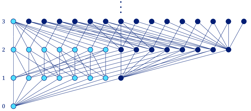
Figure 1: Hasse diagram of the set of all multispaces over $\mathbb{F}_{2}^{3}$ of rank up to $3$, partially ordered by inclusion. Subspaces of $\mathbb{F}_{2}^{3}$ are represented by light-blue nodes.

Proposition 2.7.

The number of multispaces of rank $m$ over $\mathbb{F}_{q}^{n}$ is given by

$$\left|\mathcal{M}_{q}(n,m)\right|=\sum_{k=0}^{m}\binom{n}{k}_{\!q}.$$ (2.7)

The number of multispaces covered by $W$, $\operatorname{rank}(W)\geqslant 1$, in $(\mathcal{M}_{q}(n),\subseteq)$ is

$$\mathbbm{1}(\operatorname{rank}(W)>\dim(W))+\sum_{i=0}^{\dim(W)-1}q^{i}.$$ (2.8)

The number of multispaces that cover $W$ in $(\mathcal{M}_{q}(n),\subseteq)$ is

$$1+\sum_{i=0}^{n-\dim(W)-1}q^{i}.$$ (2.9)

Proof.

By Proposition 2.3, a multispace is uniquely determined by its underlying space and its rank. In other words, every subspace of $\mathbb{F}_{q}^{n}$ of dimension $1,\ldots,m$ is the underlying space of a unique multispace of rank $m$. This fact, together with (1.1), implies (2.7).

Let us show (2.8). If $\operatorname{rank}(W)=\dim(W)$, then $W$ is a subspace of $\mathbb{F}_{q}^{n}$ and hence the multispaces it covers are the $(\dim(W)-1)$-subspaces of $W$, of which there are $\binom{\dim(W)}{\dim(W)-1}_{\!q}=\binom{\dim(W)}{1}_{\!q}=\frac{q^{\dim(W)}-1}{q-1}$ (see (1.1)). If $\operatorname{rank}(W)>\dim(W)$, then there are $\binom{\dim(W)}{1}_{\!q}+1$ multispaces of rank $\operatorname{rank}(W)-1$ covered by $W$: $\binom{\dim(W)}{1}_{\!q}$ multispaces having as the underlying space a $(\dim(W)-1)$-subspace of $\underline{W}$ and in which the multiplicity of each element is $q^{\operatorname{rank}(W)-\dim(W)}$, and $1$ multispace with $\underline{W}$ as the underlying space and with the multiplicity of each element being $q^{\operatorname{rank}(W)-\dim(W)-1}$.

(2.9) is shown in a similar way. There are $\binom{n-\dim(W)}{1}_{\!q}+1$ multispaces of rank $\operatorname{rank}(W)+1$ covering $W$: $\binom{n-\dim(W)}{1}_{\!q}$ multispaces having as the underlying space a $(\dim(W)+1)$-superspace of $\underline{W}$ and in which the multiplicity of each element is $q^{\operatorname{rank}(W)-\dim(W)}$, and $1$ multispace having $\underline{W}$ as the underlying space and with the multiplicity of each element being $q^{\operatorname{rank}(W)-\dim(W)+1}$. $\blacksquare$

Note that $\left|\mathcal{M}_{q}(n,m)\right|$ does not depend on $m$ when $m\geqslant n$, i.e.,

$$\left|\mathcal{M}_{q}(n,m)\right|=\left|\mathcal{M}_{q}(n,n)\right|=\left|\mathcal{P}_{q}(n)\right|,\quad\forall m\geqslant n.$$ (2.10)

In fact, every segment of the lattice $(\mathcal{M}_{q}(n),\subseteq)$ involving multispaces of rank $m>n$ and $m+1$, namely $(\mathcal{M}_{q}(n,m)\cup\mathcal{M}_{q}(n,m+1),\subseteq)$, is an identical copy of the segment $(\mathcal{M}_{q}(n,n)\cup\mathcal{M}_{q}(n,n+1),\subseteq)$.

A natural metric can be associated with a lattice satisfying (2.6) [1, Chapter X], namely:

$$d(W_{1},W_{2}) =\operatorname{rank}(W_{1}\lor W_{2})-\operatorname{rank}(W_{1}\land W_{2})$$ (2.11)

$$=2\operatorname{rank}(W_{1}\lor W_{2})-\operatorname{rank}(W_{1})-\operatorname{rank}(W_{2})$$

$$=\operatorname{rank}(W_{1})+\operatorname{rank}(W_{2})-2\operatorname{rank}(W_{1}\land W_{2}).$$

This distance can also be interpreted as the length of the shortest path from $W_{1}$ to $W_{2}$ in the Hasse diagram of $(\mathcal{M}_{q}(n),\subseteq)$. The next claim examines how the distance between two multispaces relates to the distance between their underlying spaces.

Proposition 2.8.

For any $W_{1},W_{2}\in\mathcal{M}_{q}(n)$,

$$d(W_{1},W_{2})\geqslant d\!\left(\underline{W_{1}},\underline{W_{2}}\right),$$ (2.12)

with equality if and only if $\operatorname{rank}(W_{1})-\operatorname{rank}(W_{2})=\dim(W_{1})-\dim(W_{2})$.

For any $W_{1},W_{2}\in\mathcal{M}_{q}(n,m)$,

$$d(W_{1},W_{2})=d(\underline{W_{1}},\underline{W_{2}})+|\dim(W_{1})-\dim(W_{2})|$$ (2.13)

and, consequently,

$$d(\underline{W_{1}},\underline{W_{2}})\leqslant d(W_{1},W_{2})\leqslant 2d(\underline{W_{1}},\underline{W_{2}}),$$ (2.14)

where equality on the left-hand side holds if and only if $\dim(W_{1})=\dim(W_{2})$, and the one on the right-hand side holds if and only if $\underline{W_{1}}\subsetneq\underline{W_{2}}$ or $\underline{W_{2}}\subsetneq\underline{W_{1}}$.

Proof.

From (2.4) we have

$$\operatorname{rank}(W_{1}\cap W_{2})$$ (2.15)

$$=\dim\!\left(W_{1}\cap W_{2}\right)+\min\!\big{\{}\operatorname{rank}(W_{1})-\dim(W_{1}),\,\operatorname{rank}(W_{2})-\dim(W_{2})\big{\}}$$

$$\leqslant\dim\!\left(W_{1}\cap W_{2}\right)+\frac{1}{2}\big{(}\operatorname{rank}(W_{1})-\dim(W_{1})+\operatorname{rank}(W_{2})-\dim(W_{2})\big{)}$$

and hence

$$d(W_{1},W_{2}) =\operatorname{rank}(W_{1})+\operatorname{rank}(W_{2})-2\operatorname{rank}(W_{1}\land W_{2})$$ (2.16)

$$\geqslant\dim(W_{1})+\dim(W_{2})-\dim(W_{1}\cap W_{2})$$

$$=\dim\!\left(\underline{W_{1}}\right)+\dim\!\left(\underline{W_{2}}\right)-\dim\!\left(\underline{W_{1}}\cap\underline{W_{2}}\right)$$

$$=d\!\left(\underline{W_{1}},\underline{W_{2}}\right).$$

Equality in (2.16), or equivalently (2.15), holds if and only if $\operatorname{rank}(W_{1})-\dim(W_{1})+\operatorname{rank}(W_{2})-\dim(W_{2})=2\min\{\operatorname{rank}(W_{1})-\dim(W_{1}),\,\operatorname{rank}(W_{2})-\dim(W_{2})\}$,i.e., $\operatorname{rank}(W_{1})-\dim(W_{1})=\operatorname{rank}(W_{2})-\dim(W_{2})$.

When $W_{1},W_{2}\in\mathcal{M}_{q}(n,m)$, we have $\min\{\operatorname{rank}(W_{1})-\dim(W_{1}),\,\operatorname{rank}(W_{2})-\dim(W_{2})\}=m-\max\{\dim(W_{1}),\,\dim(W_{2})\}$. Suppose, without loss of generality, that $\dim(W_{1})\geqslant\dim(W_{2})$. We then have

$$d(W_{1},W_{2}) =2\big{(}m-\operatorname{rank}(W_{1}\land W_{2})\big{)}$$ (2.17)

$$=2\big{(}\max\{\dim(W_{1}),\,\dim(W_{2})\}-\dim\!\left(\underline{W_{1}}\cap\underline{W_{2}}\right)\big{)}$$

$$=2\big{(}\dim\!\left(\underline{W_{1}}\right)-\dim\!\left(\underline{W_{1}}\cap\underline{W_{2}}\right)\big{)}$$

$$=\dim\!\left(\underline{W_{1}}\right)+\dim\!\left(\underline{W_{2}}\right)-2\dim\!\left(\underline{W_{1}}\cap\underline{W_{2}}\right)+\dim\!\left(\underline{W_{1}}\right)-\dim\!\left(\underline{W_{2}}\right)$$

$$=d(\underline{W_{1}},\underline{W_{2}})+|\dim(W_{1})-\dim(W_{2})|.$$

Inequalities (2.14) are now obvious. $\blacksquare$

The graph $\Gamma_{q}(n,m)$ associated with the metric space $(\mathcal{M}_{q}(n,m),d)$ is obtained by joining by an edge any two nodes/multispaces that are at distance $2$ (the distance between multispaces of the same rank is necessarily even, see (2.13)). The graph $\Gamma_{q}(n,m)$ contains as subgraphs the Grassmann graphs corresponding to $(\mathcal{G}_{q}(n,k),d)$, $k=1,\ldots,m$. Unlike Grassmann graphs, however, $\Gamma_{q}(n,m)$ is not distance-regular.

3 Multispace Codes

In this section we illustrate an application of multispaces in coding theory. The main purpose of this discussion is to present the framework for multispace codes and their applications, leaving a more in depth investigation of such codes for future work.

Subspace codes are codes in $\mathcal{P}_{q}(n)$; when restricted to $\mathcal{G}_{q}(n,k)$, they are called constant-dimension subspace codes. These objects were introduced in [5] as appropriate constructs for error correction in communication channels that deliver to the receiver random linear combinations of the transmitted vectors from $\mathbb{F}_{q}^{n}$. A practical instantiation of such a channel would be a network whose nodes/routers forward on their outgoing links random linear combinations of the incoming vectors/packets, a paradigm known as ‘random linear network coding’ [3]. Given a channel of this kind, one naturally comes to the idea that information the transmitter is sending should be encoded in an object that is invariant (with high probability) under random linear transformations, namely a vector subspace of $\mathbb{F}_{q}^{n}$. A code for such a channel should therefore be defined in $\mathcal{P}_{q}(n)$ and should, as always, satisfy certain minimum distance requirements in order for the receiver to be able to correct a certain number of errors. The way of measuring the distance between subspaces depends on the details of the model, but the most common choice is precisely the metric (2.11). In the described setting, the transmitter would typically send a basis of the selected codeword/subspace through the channel, and the receiver’s task would be to reconstruct the codeword from the received vectors.

We propose the use of codes in $\mathcal{M}_{q}(n)$ for the same purpose. The scenario we have in mind is the following: the transmitter sends a generating multiset $B$ of the selected codeword/multispace $W$ (over $\mathbb{F}_{q}^{n}$), and the channel delivers to the receiver a multiset $B^{\prime}$ of random linear combinations of the transmitted vectors. Note that multiple copies of the same packet/vector can easily be generated, so the assumption that the transmitter sends a multiset of vectors is physically well-justified and quite natural in this context. The scenario just described was in fact the motivation for defining multispaces as in Definition 2.2. It follows from Proposition 2.4 that, if the channel action is represented by a full-rank $\operatorname{rank}(W)\times\operatorname{rank}(W)$ matrix, then the transmitted multispace is preserved in the channel, i.e., the receiver will reconstruct it perfectly from the received multiset $B^{\prime}$. In general, however, the channel may introduce errors. We next show that two reasonable types of errors in this context – deletions and dimension-reductions – result in the received multispace that is at a bounded distance, depending only on the number of errors, from the transmitted multispace. Consequently, one can design a code in $\mathcal{M}_{q}(n)$ that is guaranteed to correct a given number of errors by specifying its minimum distance with respect to the metric (2.11).

Proposition 3.1.

Let $\boldsymbol{b^{\prime}}=\boldsymbol{b}T$, where $\boldsymbol{b}=(b_{1},\ldots,b_{m})$, $\boldsymbol{b^{\prime}}=(b^{\prime}_{1},\ldots,b^{\prime}_{m^{\prime}})$, $b_{i},b^{\prime}_{i}\in\mathbb{F}_{q}^{n}$, and $T$ is an $m\times m^{\prime}$ matrix over $\mathbb{F}_{q}$. Denote also $B=\{\mskip-6.0mu\{b_{1},\ldots,b_{m}\}\mskip-6.0mu\}$, $B^{\prime}=\{\mskip-6.0mu\{b^{\prime}_{1},\ldots,b^{\prime}_{m}\}\mskip-6.0mu\}$.
(1) If $m^{\prime}=m-s$ and $\operatorname{rank}T=m^{\prime}$, then $d(\operatorname{mspan}_{q}(B),\operatorname{mspan}_{q}(B^{\prime}))=s$.
(2) If $m^{\prime}=m$ and $\operatorname{rank}T=m-s$, then $d(\operatorname{mspan}_{q}(B),\operatorname{mspan}_{q}(B^{\prime}))\leqslant 2s$.

Proof.

We think of $B$, $B^{\prime}$ as the transmitted and the received multisets of vectors, respectively, and of $W=\operatorname{mspan}_{q}(B)$, $W^{\prime}=\operatorname{mspan}_{q}(B^{\prime})$ as the corresponding multispaces.

(1) The channel action (i.e., the action of the operator $T$) can in this case be thought of as first transforming $\boldsymbol{b}$ to $\boldsymbol{\tilde{b}}$ by a full-rank $m\times m$ matrix, and then transforming $\boldsymbol{\tilde{b}}$ to $\boldsymbol{b^{\prime}}$ by deleting $s$ of the former’s coordinates. We know from Proposition 2.4 that $W=\tilde{W}$. Also, it is straightforward to see that deleting $s$ elements of the generating multiset $\tilde{B}$, i.e., $B^{\prime}\subseteq\tilde{B}$, $|B^{\prime}|=|\tilde{B}|-s$, results in a multispace $W^{\prime}$ which is contained in $\tilde{W}$ and whose rank is $\operatorname{rank}(W^{\prime})=\operatorname{rank}(\tilde{W})-s$. Therefore, under the stated assumptions, $W\land W^{\prime}=W^{\prime}$, and hence $d(W,W^{\prime})=s$.

(2) This scenario corresponds to the case when the channel delivers $m$ vectors to the receiver (as many as were transmitted), but the transformation is not full-rank. A simple linear algebra shows that, under these assumptions, $\dim(W^{\prime})\geqslant\dim(W)-s$. Since also $W^{\prime}\subseteq W$ and $\operatorname{rank}(W)=\operatorname{rank}(W^{\prime})=m$, we conclude from Proposition 2.8 that $d(W,W^{\prime})\leqslant 2s$. $\blacksquare$

The main advantage of the transition from subspaces to multispaces that is proposed here is that the code space is in the latter case infinitely larger – $\mathcal{M}_{q}(n)$ instead of $\mathcal{P}_{q}(n)$. In particular, if the parameters $n$ and $q$ (which, in the network coding scenario, correspond to packet length and alphabet size, respectively) are fixed, subspace codes are necessarily bounded, both in cardinality and minimum distance. This fact stands in sharp contrast to most other communication scenarios in which codes of arbitrarily large cardinality and minimum distance exist even over a fixed alphabet. With multispaces on the other hand, taking, say, $\bigcup_{j=0}^{m}\mathcal{M}_{q}(n,j)$ as the code space, one can consider the asymptotic regime $m\to\infty$ even if $n$ and $q$ are fixed. In this regime the size of the code space scales as

$$\sum_{j=0}^{m}|\mathcal{M}_{q}(n,j)|\;\sim\;m\cdot\sum_{k=0}^{n}\binom{n}{k}_{\!q}$$ (3.1)

(see (2.7)) and is unbounded.

To conclude the paper, we again emphasize that the aim of the brief discussion in this section was to introduce the notion of multispace codes – a generalization of subspace codes – and argue that they can be used in the same scenarios as subspace codes, with an important advantage that they are capable of achieving larger (in some cases infinitely larger) information rates. Further work on the subject would entail devising concrete constructions of codes in $\bigcup_{j=0}^{m}\mathcal{M}_{q}(n,j)$ having a desired minimum distance, and deriving bounds on the parameters of optimal such codes (similar to those in, e.g., [2]). We note that certain bounds, namely sphere-packing and Singleton bounds, on codes in modular lattices have already been studied in [4].