High fidelity two-qubit quantum state tomography of Electron-¹⁴N hybrid spin register in diamond

Abstract

We report here on a major improvement of the control and characterization capabilities of ¹⁴N nuclear spin of single NV centers in diamond, as well as on a new method that we have devised for characterizing quantum states, i.e. quantum state tomography using Rabi experiments. Depending on whether we use amplitude information or phase information from Rabi experiments, we define two sub-methods namely Rabi amplitude quantum state tomography (RAQST) and Rabi phase quantum state tomography (RPQST). The advantage of Rabi-based tomography methods is that they lift the requirement of unitary operations used in other methods in general and standard methods in particular. On one hand, this does not increase the complexity of the tomography experiments in large registers, and on the other hand, it decreases the error induced by MW irradiation. We used RAQST and RPQST to investigate the quality of various two-qubit pure states in our setup. As expected, test quantum states show very high fidelity with the theoretical counterpart. The best fidelity, i.e. 0.9995, is achieved for state $|{\psi}\rangle=0.9008|{00}\rangle+(-0.1556-0.4054i)|{-11}\rangle$ using RPQST. We tested our method on a total of three two-qubit pure states and found an average fidelity of 0.9973 using RPQST and 0.9856 using RAQST.

I Introduction

The importance of quantum computation (QC) is boosting by recent demonstrations towards the quantum advantage Arute et al. (2019); Zhong et al. (2020); Ristè et al. (2017); Morvan et al. (2023) as well as by approaching applications ranging from science and technology to daily life Andreas et al. (2021). This has motivated researchers for the experimental implementation of various quantum algorithms in search for the most efficient methodologies for characterizing quantum systems. These algorithms, typically known as the quantum state tomography and quantum process tomography, are at the heart of engineering favorable quantum states. There are various quantum computing architectures Nielsen and Chuang (2010), some of which have shown encouraging growth in achieving intermediate-scale quantum registers and in the deployment of noisy intermediate-scale quantum computers. The solid-state spin-based architecture, which has been considered highly interesting due to its compatibility with microelectronic systems, still needs to demonstrate its potential. Among all available solid-state spin-based candidates for QC, the nitrogen-vacancy (NV) center in diamond is in the lead, thanks to its peculiar characteristics such as room temperature initialization and detection using optical pumping, better coherence time to gate time ratio, and ultimately important miniaturizing abilities Stolze and Suter (2008). Besides the scalability, an important requirement of a quantum circuit is the ability to apply gates with a small enough error to allow the application of error correction codes. Here, solid-state spin systems turned out to be more suitable for fault-tolerant computation due to their weak coupling with the environment and a robust electromagnetic field control Hanson et al. (2008). These characteristics make NV centers an eligible candidate for desktop QC if the scalability bottleneck can be broken Fehler et al. (2019). This important scalability issue is addressed in ongoing works, particularly by trying to couple close NV spins using different pathways, like optically mediated coupling based on spin-photon interface or reading dipole-dipole coupling electrically Siyushev et al. (2019); Ruf et al. (2021).

Moreover the scalability only is not sufficient. The first step in developing such quantum computers is improving fidelity of two-qubit gates. To take full advantage of the NV solid state quantum register, here we focus on deterministic qubit state engineering. In particular, we develop novel quantum state tomography and control techniques in order to reach the highest fidelity. The aim of the current work is two-fold: 1) demonstrating the state-of-the-art control, noise minimization, and error mitigation by high-fidelity state preparation, 2) presenting a new scheme for quantum state tomography with the aim of minimizing the number of experiments.
In NV center systems, the availability of additional nuclear spins allows to make use of a relatively easier approach in achieving a larger spin register and also a nuclear spin network coupled through dipolar-dipolar interaction and addressed using electron-nuclear spin gates. We use this electron-nuclear spin gate to address nuclear spin states in order to be able to dress spin states.

An NV center is a point defect in the diamond lattice consisting of a substitutional nitrogen atom and a neighboring vacancy. It can be neutral, NV⁰, negatively, NV^- or positively NV⁺ charged. The NV^- has a spin triplet ground state - two of its electrons are unpaired. NV^- (further referred to as "NV" in this article ) possesses an electron spin and a ¹⁴N nuclear spin, both of which are spin 1 systems forming a 9-dimensional Hilbert space of e-¹⁴N composite spin systems. Exploiting universal control and careful readout of only the desired subspace, it is possible to prepare an arbitrary quantum state over a reduced 4-dimensional Hilbert space corresponding to two two-level spin subsystems, of which the electronic spin is used as a probe by measuring optically detected magnetic resonance. The e-¹⁴N hybrid spin system Hamiltonian, along with experimental details, are described in the Sec. III. The e-¹⁴N spin systems described here are connected through the longitudinal part of the hyperfine coupling defined by the last term of the Eq. 10 in Sec. III. Taking the initialization procedure from Chakraborty et al. (2017) as a base, we modify and optimize the sequence that allows us to initialize both electron and nuclear spins to $m_{s}=0,m_{I}=0$ signified as the $|{0,0}\rangle$ state. We further prepare an arbitrary initial single-qubit state on the nuclear spin and entangle it with the NV electron spin-qubit. Further on, we tomograph the two-qubit quantum state using a novel Quantum State Tomography (QST) method to characterize the full quantum state, discussed below II.

Quantum state tomography (QST) reveals full information about the quantum state on which tomography is performed. For the pure quantum state, QST reveals information about the tilt angle $\theta$ and phase $\phi$ in the quantum state described in Eq. 3, while for the mixed state, QST reveals information about the population and off-diagonal coherence terms. The best fidelity we could achieve for our two-qubit pure quantum state among all our test quantum states is 0.9995 and to the best of our knowledge is the highest quoted fidelity prepared using electron-nuclear two-qubit spin gates, even though we do not use advanced techniques such as optimal control theory and dynamical decoupling (DD) for protection against decoherence. The new methodology that we have devised for QST involves just two Rabi experiments used to characterize the quantum state. We call this method Rabi Quantum State Tomography (RQST). Furthermore, RQST has two variants: Rabi amplitude quantum state tomography (RAQST) and Rabi phase quantum state tomography (RPQST) depending on whether amplitude or phase information of the Rabi oscillation is used for extracting quantum state parameters.

II Rabi quantum state tomography

The most general qubit quantum state $|{\psi}\rangle$ can be described in the Pauli operator basis $\{\mathbb{I},\sigma_{x},\sigma_{y},\sigma_{z}\}$ as

$$\rho = \frac{1}{2}(\mathbb{I}+(\langle{\sigma_{x}}\rangle\sigma_{x}+\langle{\sigma_{y}}\rangle\sigma_{y}+\langle{\sigma_{z}}\rangle\sigma_{z})$$ (1)

$$= \frac{1}{2}(\mathbb{I}+(n_{x}\sigma_{x}+n_{y}\sigma_{y}+n_{z}\sigma_{z})$$ (2)

Here, $n_{x}$, $n_{y}$, and $n_{z}$ are the coordinates of the Bloch vector tip. The characterization of the quantumm state is equivalent to calculating the coordinates of the point coinciding with the tip of the Bloch sphere, i.e. $n_{x}$, $n_{y}$, and $n_{z}$. Alternatively, the pure state $|{\psi}\rangle$ is described as

$$|{\psi}\rangle=\cos{\frac{\theta}{2}}|{0}\rangle+e^{i\phi}\sin{\frac{\theta}{2}}|{1}\rangle.$$ (3)

where quantities $\theta$ and $\phi$ are respectively the azimuthal and polar angle in the Bloch sphere representation.

The standard method of QST of an arbitrary dimension state involves the readout of all directly observable terms (for NV centers, this means $\sigma_{z}$ terms of the electron spin state), followed by the transfer of unobservable terms (for NV centers $\langle{\sigma_{x}}\rangle$ and $\langle{\sigma_{y}}\rangle$ for electron spin and all nuclear spin terms) into observable terms and reading them out. In our radically different approach, we use two Rabi experiments to determine the quantum state fully. There are multiple ways to extract $\langle{\sigma_{x}}\rangle$, $\langle{\sigma_{y}}\rangle$, $\langle{\sigma_{z}}\rangle$ from Rabi experiments. In particular, our first RAQST method uses the amplitudes of the Rabi oscillations for quantum state reconstruction and the second method (RPQST) uses only the phases of the X and Y Rabi oscillations for quantum state reconstruction.

Figure 1: Bloch sphere representation of unknown state $|{\psi}\rangle$ with Cartesian coordinates system, let’s call it state coordinates $n_{x},n_{y},n_{z}$ and spherical coordinate system $\theta$ and $\phi$. The pure state is represented by the Bloch vector with the tip of the vector on the surface of the Bloch sphere and the mixed state is represented by the Bloch vector with the tip inside the Bloch sphere.

The spherical geometry of the Bloch sphere gives rise to the following relations between state coordinates

$$n_{x}^{2} = \left(\frac{A_{y}}{A_{\text{ref}}}\right)^{2}-n_{z}^{2},$$ (4)

$$n_{y}^{2} = \left(\frac{A_{x}}{A_{\text{ref}}}\right)^{2}-n_{z}^{2},$$

$$n_{z}^{2} = \left(\frac{A_{x}}{A_{\text{ref}}}\right)^{2}+\left(\frac{A_{y}}{A_{\text{ref}}}\right)^{2}-1.$$

Here $A_{x}$, $A_{y}$ are the amplitudes of the rabi oscillations around x- and y-axes respectively. $A_{ref}$ is the amplitude of the rabi oscillation performed on an eigenstate. However, Eq. 4 does not uniquely specify the coordinates but rather narrows down possibilities to 8 points on the Bloch sphere, as can be seen on figure 2. Additional information has to be obtained from the phase of the Rabi oscillations (see supplementary information). The link between these phases and the Rabi oscillations depend on the link between measured PL and the base states on the Bloch sphere.

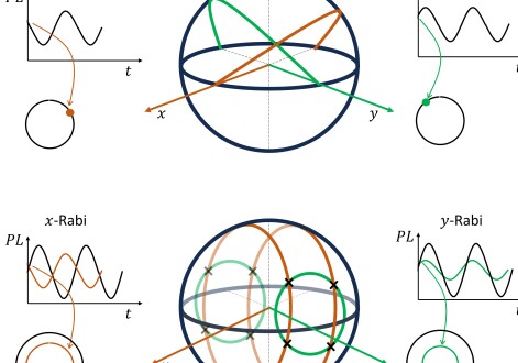
Figure 2: Schematic presentation of the quantum state tomography (QST) based on the Rabi cycle. In the center is the Bloch sphere, a single point on which represents a superposition state of two-level system unequivocally. First Rabi measurement (left) narrows down the possibilities to a single (brown) line. The intersection point with the similar (green) line from a 90° shifted Rabi measurement (right) is the result of the tomography. (a) Phase Rabi QST. (b) Amplitude Rabi QST.

After considering this phase information we can uniquely determine coordinates $\{n_{x},n_{y},n_{z}\}$. The azimuthal angle $\theta$ and the polar angle $\phi$ used in the Eq. 3 are related with the coordinates $n_{x}$, $n_{y}$, and $n_{z}$ by the following formulae:

$$\theta=\operatorname{\tan^{-1}}{\left(\frac{\sqrt{n_{x}^{2}+n_{y}^{2}}}{n_{z}}\right)}+\frac{\pi}{2}$$ (5)

$$\phi=\pi-\operatorname{\tan^{-1}}{\left(\frac{n_{x}}{n_{y}}\right)}-\frac{n_{y}}{|n_{y}|}\frac{\pi}{2}.$$ (6)

Figure 3: Figure consists of a Bloch sphere picture, top view, x-Rabi, and y-Rabi. Subplots for x-Rabi and y-Rabi are depicting initial phases $\alpha$ and $\beta$, showing their relation with $\phi$ and $\theta$

.

RAQST requires a reference Rabi experiment to learn the largest Rabi amplitude, as the Bloch sphere is normalized. Comparison of amplitudes ($A_{x}$ and $A_{y}$) of x-Rabi and y-Rabi measurements of an unknown state with the reference ($A_{\text{ref}}$) gives information about the state. In order to overcome the requirement of a reference experiment in RAQST we develop the RPQST method.

Rabi phase tomography (RPQST) does not require a reference measurement, also it requires only the phases of the two Rabi oscillations to identify the Bloch vector coordinates completely, as can be seen on figure 2. Figure 3 introduces angles $\alpha$ and $\beta$, which are extracted directly from Rabi measurements. We exploit the advantage of spherical geometry of the Bloch sphere to derive the relation between the angles $\theta$ and $\phi$ of the state to be tomograph with the phases of Rabi oscillations $\alpha$ and $\beta$, that is

$$\theta=\frac{\cos{\alpha}}{|\cos{\alpha}|}[|\operatorname{\tan^{-1}}(\frac{\tan{\alpha}}{\cos{\phi}})|-\frac{\pi}{2}]+\frac{\pi}{2}$$ (7)

$$\phi=\pi-\operatorname{\tan^{-1}}(\frac{\tan{\beta}}{\tan{\alpha}})-\frac{\sin{\alpha}}{|\sin{\alpha}|}\frac{\pi}{2}$$ (8)

Experimentally, both RAQST and RPQST have their advantages and drawbacks. For example, because RAQST uses a reference measurement, the obtained coordinates can be verified using this redundant information. On the other hand, the amplitude of the Rabi oscillations is susceptible to experimental conditions. For example, when measuring on a single defect, it can drift out of focus during one of the three Rabi measurements. This means that the amplitude of that particular measurement will be lower than it should be. The phase of the Rabi measurements is less affected by this sample drift and is, therefore, more useful when it’s difficult to keep the defect in focus.

In the following, we provide a quantum circuit describing our method for initializing the two-qubit hybrid spin register to state $|{0,0}\rangle$ (upper trace of Fig. 4) and a quantum circuit for our QST method (lower trace of Fig. 4). We also describe all the gates used as conditional operations in their operator form.

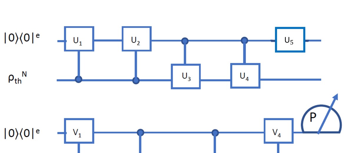
Figure 4: Upper trace: Quantum circuit for initialization of electron-nuclear spin two-qubit hybrid register to the state $|{0,0}\rangle$. Lower trace: Preparation of nuclear spin qubit to the state $|{\psi}\rangle$ and operation for performing Rabi Oscillation for a given phase $\zeta$.

The operators used in the circuit for initialization of the nuclear states to state $|{0,0}\rangle$ in the upper trace of Fig. 4 are given as follows.
$U_{1}:\operatorname{I_{3}}\otimes|{0}\rangle\langle{0}|+\operatorname{I_{3}}\otimes|{1}\rangle\langle{1}|+(|{1}\rangle\langle{0}|+|{0}\rangle\langle{1}|+|{-1}\rangle\langle{-1}|)\otimes|{-1}\rangle\langle{-1}|$

$U_{2}\colon\operatorname{I_{3}}\otimes|{0}\rangle\langle{0}|+\operatorname{I_{3}}\otimes|{-1}\rangle\langle{-1}|+(|{1}\rangle\langle{1}|+|{-1}\rangle\langle{0}|+|{0}\rangle\langle{-1}|)\otimes|{1}\rangle\langle{1}|$

$U_{3}\colon|{-1}\rangle\langle{-1}|\otimes\operatorname{I_{3}}+|{-1}\rangle\langle{-1}|\otimes\operatorname{I_{3}}+|{1}\rangle\langle{1}|\otimes(|{0}\rangle\langle{-1}|+|{-1}\rangle\langle{0}|+|{1}\rangle\langle{1}|)$

$U_{4}\colon|{1}\rangle\langle{1}|\otimes\operatorname{I_{3}}+|{0}\rangle\langle{0}|\otimes\operatorname{I_{3}}+|{-1}\rangle\langle{-1}|\otimes(|{0}\rangle\langle{1}|+|{1}\rangle\langle{0}|+|{-1}\rangle\langle{-1}|)$

$U_{5}\colon(|{0}\rangle\langle{0}|+|{0}\rangle\langle{1}|+|{0}\rangle\langle{-1}|)\otimes\operatorname{I_{3}}$
After the initialization of the electron-nuclear spin system to the state $|{0,0}\rangle$, the lower part of the circuit (see Fig. 4) illustrates the preparation of the state to be tomographed followed by a definite phase Rabi experiment. Here, we first transfer electron spin from state $|{0}\rangle$ to $|{-1}\rangle$ conditional to the nuclear spin state $|{0}\rangle$ using operator
$V_{1}\colon(|{-1}\rangle\langle{0}|+|{0}\rangle\langle{-1}|+|{1}\rangle\langle{1}|)|{0}\rangle\langle{0}|+\operatorname{I_{3}}\otimes|{1}\rangle\langle{1}|+\operatorname{I_{3}}\otimes|{-1}\rangle\langle{-1}|$.
We apply conditional gate operations for the preparation of the desired quantum state $|{\psi}\rangle$ on the nuclear spin and for executing nuclear Rabi operations. These two operations are limited to the nuclear spin subspace (i.e., $|{1}\rangle$, $|{0}\rangle$) of the electron spin subspace $|{-1}\rangle$ in the two-dimensional Hilbert space. The measurement is carried out in the $|{0}\rangle$ electron spin subspace. We can then consider the dynamics of the two-qubit register effectively limited to the subspace ($|{0,1}\rangle,|{0,0}\rangle,|{-1,1}\rangle,|{-1,0}\rangle$) to describe the dynamics without loss of generality. After the application of the $V_{1}$ operator, the quantum system is in the state $|{-1,0}\rangle$. We then prepare a quantum state $|{\psi}\rangle$ with tilt angle $\theta$ and phase $\phi$ by using operator $V_{2}$ as shown in the lower trace of Fig. 4. The state now becomes

$$\cos{\frac{\theta}{2}}|{0,0}\rangle+e^{i\phi}\sin{\frac{\theta}{2}}|{-1,1}\rangle$$ (9)

Furthermore, parametric gate $V_{3}$ is used for applying the Rabi operation conditional to electron spin subspace $|{-1}\rangle$, and ultimately nuclear and electron spin states are entangled by selectively flipping the electron spin state while nuclear spin is in state $|{0}\rangle$ only. This is modeled as a controlled operation $V_{4}$, controlled by nuclear spin states and electron spin as the target. The electron spin population is then read out using the standard procedure, i.e. using an optical detection pulse. As an example, the tomography experiments (x and y-phase Rabi experiments combined) 6 and the reconstructed density matrices Fig. 7 for the state $|{\psi}\rangle=0.9008|{-1,0}\rangle+(-0.1556-0.4054i)|{-1,1}\rangle$ for $\theta=51.48^{o}$ and $\phi=249^{o}$. We have performed a few more experiments in order to examine the efficacy of our tomography method and the fidelity results are illustrated in the table Tab. IV while the details of the experimental results are provided in the supplementary material Shukla et al. (2022). Operations $V_{2}$ and $V_{3}$ are defined as follows:
$V_{2}$$:|{0}\rangle\langle{0}|\otimes\operatorname{I_{3}}+|{1}\rangle\langle{1}|\otimes\operatorname{I_{3}}+|{-1}\rangle\langle{-1}|\otimes e^{(-\iota\theta I_{\phi})}$, where $I_{\phi}=\cos{\phi}I_{x}+\sin{\phi}I_{y}$.
$V_{3}$$:|{0}\rangle\langle{0}|\otimes\operatorname{I_{3}}+|{1}\rangle\langle{1}|\otimes\operatorname{I_{3}}+|{-1}\rangle\langle{-1}|\otimes e^{(-\iota\theta(t)I_{\zeta})}$.
In the above $I_{x},I_{y}$ are spin angular momentum operators for a two-level system.

III Experimental implementation of Rabi quantum state tomography

We demonstrate the Rabi tomography method on the nuclear spin of an NV center. The electron-nuclear system of the NV center without considering strain is described by the Hamiltonian

$$H=2\pi\hbar(DS_{z}^{2}+\gamma_{e}B_{o}S_{z}+PI_{z}^{2}+\gamma_{N}B_{o}I_{z}+AS_{z}I_{z})$$ (10)

Here, D is the zero-field splitting (ZFS), $\gamma_{e}B_{o}$ is the Zeeman splitting of electron spins, P is the quadrupolar splitting, $\gamma_{N}B_{o}$ is the Zeeman splitting of nuclear spins, A is the longitudinal part of the hyperfine coupling between electron and ¹⁴N nuclear spin. The three levels of the electron spin-1 system are the lowest vibronic levels out of which a two-level system can be derived, say $m_{s}=0$ for the ground vibronic state and $m_{s}=1$ for the excited vibronic state. The optical response of the NV center depends on the respective population of these states, which allows to perform the readout operation. Similarly, the qubit subspace {$m_{I}=0,m_{I}=1\}$ from the nuclear spin state space can be derived. The respective population of nuclear states, however, has no influence on the optical response, therefore the nuclear spin state is not considered directly observable. These two pairs of states are the computational states in our algorithm. Quantum mechanically these two populations are comprised of expectation values of the $\sigma_{z}$ operator. Thus, $\sigma_{z}$ of the electron spin is the directly observable term which we determine through Rabi.

In order to demonstrate the validity of tomography results we perform it on a known arbitrary state of the nuclear spin. This means that the state has to be prepared in advance. The first step to state preparation is initialization to the eigenstate. While the electron spin can be initialized to $m_{S}=0$ with a laser pulse, the nuclear spin does not have such an intrinsic initializing mechanism. On the contrary, a strong enough laser pulse can destroy the initialization of the nuclear spin, making the three states of the nuclear spin triplet equally populated. We choose as a procedure for nuclear spin initialization a sequence of transition selective pulses Chakraborty et al. (2017). Figure 5-top shows the principle of the sequence operation. A laser pulse initializes the electron spin, two microwave (MW) pulses drive two-electron spin transitions, and then the radio-frequency (RF) pulse drives two nuclear spin transitions, followed by another shorter laser pulse, which initializes electron spin to $m_{S}=0$ again. The duration of the last laser pulse is crucial since it has to preserve the nuclear spin polarization. MW and RF pulses have to exactly invert the population (a $\pi$-pulse), therefore the optimal duration, as well as the exact frequency of these pulses, also had to be determined in advance (See supplementary material Shukla et al. (2022) for details of initialization and optimization of optical and RF pulses).

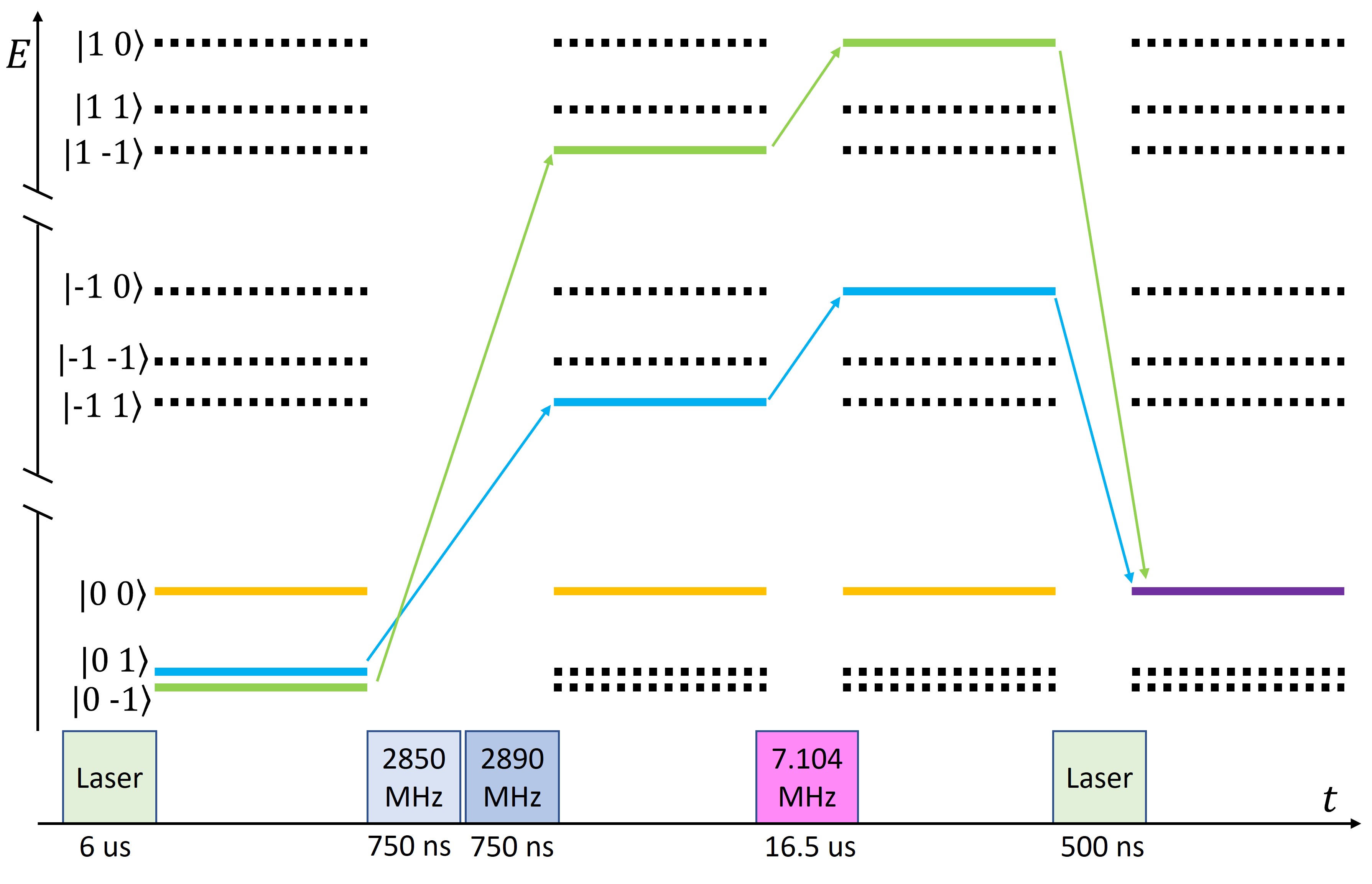
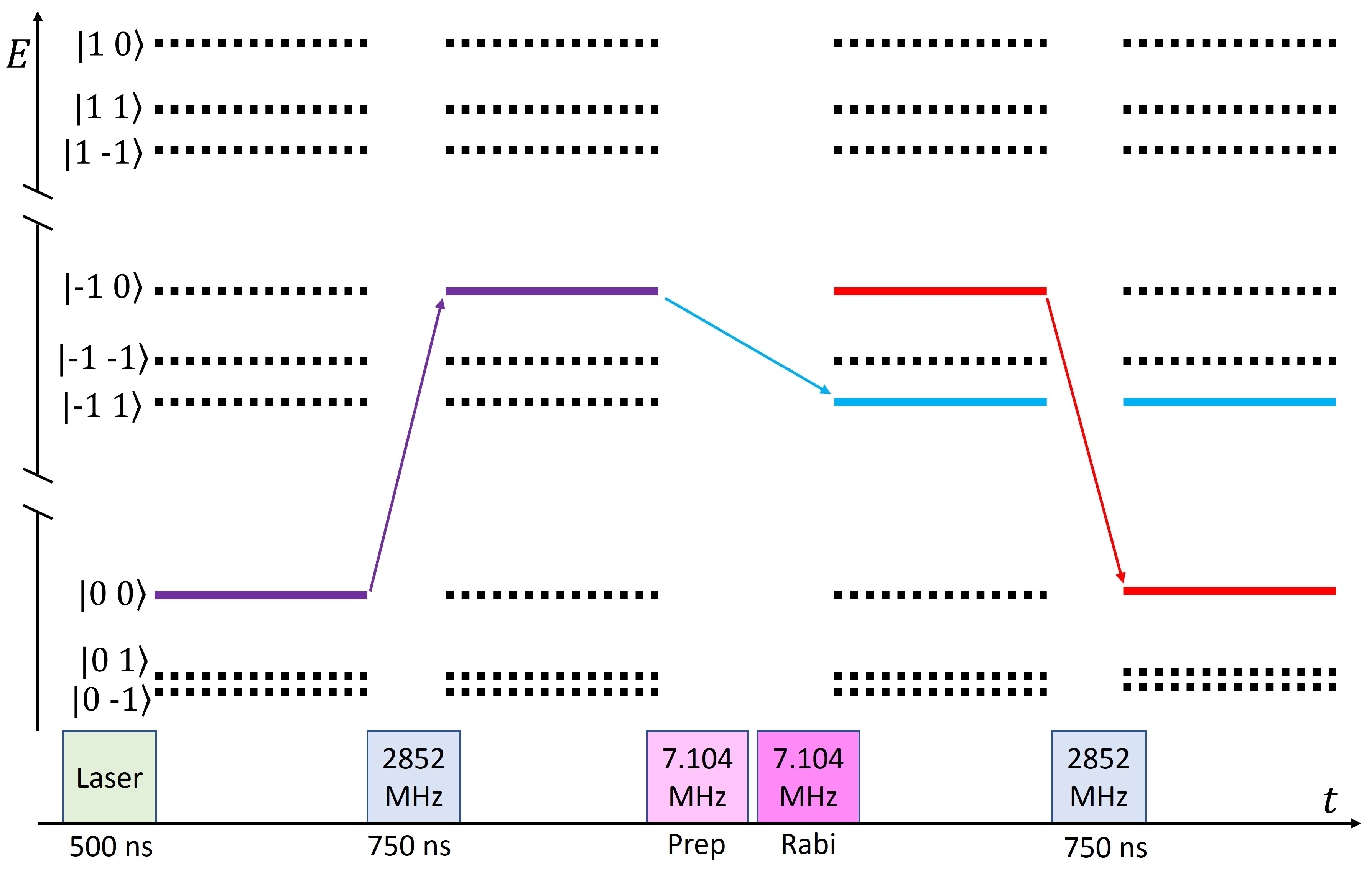
Figure 5: Action of the elements of the initialization (top) and Rabi tomography (bottom) sequences on NV center states. The states are written in the format $|{m_{S},m_{I}}\rangle$. Dashed lines represent empty states, and solid-colored lines represent populated states. Different coloring of the states is to guide the eye. The 7.11 MHz RF pulses in the Rabi tomography sequence are the preparation of an arbitrary state (Prep) and the pulse of variable duration that performs the Rabi cycle (Rabi). The two RF pulses are not phase-matched, but have a well defined phase difference.

Once the nuclear spin is initialized to the eigenstate, an arbitrary state needs to be prepared. For that reason, we drive the transition between $m_{I}=0$ and $m_{I}=1$ for an arbitrary period of time with the preparation RF pulse. At $m_{s}=0$ the nuclear levels $m_{I}=1$ and $m_{I}=-1$ are not well resolved, therefore preceding the preparation pulse is the electron spin transition $m_{S}=0$ to $m_{S}=-1$ (figure 5-bottom). Once the state has been prepared to an arbitrary state, an x-phase or y-phase RF pulse of varying duration drives the Rabi cycle between $m_{I}=0$ and $m_{I}=1$. After that, the population of $|{-1,0}\rangle$ (in the notation $|{m_{S},m_{I}}\rangle$) is transferred to $|{0,0}\rangle$ with the MW pulse, where it can be read. The full sequence has to be repeated for each duration of the Rabi pulse to obtain the Rabi oscillations signal.

IV Results and discussion

First, the RAQST protocol is tested using a generic state

$$|{\psi}\rangle=\cos\left(\frac{\theta}{2}\right)|{0}\rangle+e^{i\phi}\sin\left(\frac{\theta}{2}\right)|{1}\rangle$$ (11)

with $\theta=58.41^{\circ}$ and $\phi=249^{\circ}$. The theoretical density operator for this state is

$$\rho_{th}=\frac{1}{2}\left[\begin{array}[]{cc}1.52&-0.31+0.80i\\ -0.31-0.80i&0.48\\ \end{array}\right]$$

Using the amplitudes of the recorded Rabi cycles (figure 6), the values $\theta=50.3479^{\circ}$ and $\phi=242.0980^{\circ}$ are found. Thus, the experimental recovered density operator using the amplitude of Rabi oscillations is

$$\rho_{exp,A}=\frac{1}{2}\left[\begin{array}[]{cc}1.64&-0.36+0.68i\\ -0.36-0.68i&0.36\\ \end{array}\right]$$

While the density operator recovered with the phase of Rabi oscillations is

$$\rho_{exp,P}=\frac{1}{2}\left[\begin{array}[]{cc}1.49&-0.3209+0.81i\\ -0.32-0.8120i&0.45\\ \end{array}\right].$$

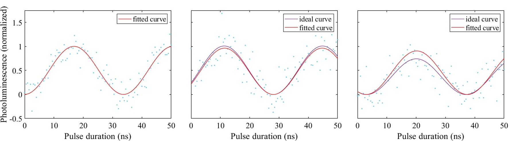
Figure 6: Nuclear Rabi tomography experiment results for the state ($\theta=58.41^{\circ}$, $\phi=249^{\circ}$) and the reference measurement. Experimental data is fitted (red) and expanded with the Rabi oscillations to be expected (purple) for the ideal state ($\theta=58.41^{\circ}$, $\phi=249^{\circ}$). The amplitudes of the theoretically expected and experimentally measured Rabi oscillations differ to a higher degree than their respective phases, leading to the lower fidelity obtained with RAQST.

The measured density operators both look quite similar to the ideal case $\rho_{th}$, which can be seen in the 3D bar plot of these density operators Fig. 7. The fidelity, $F$, of the different density operators is calculated via the formula

$$F=\frac{\text{Tr}(\rho_{th}\rho_{exp})}{\sqrt{\text{Tr}(\rho_{th}^{2})\text{Tr}(\rho_{exp}^{2})}}\,.$$ (12)

Using the obtained density operators, a fidelity of $F_{A}=0.9927$ is determined for the presented RAQST measurement and a fidelity of $F_{P}=0.9995$ is for the presented RPQST.

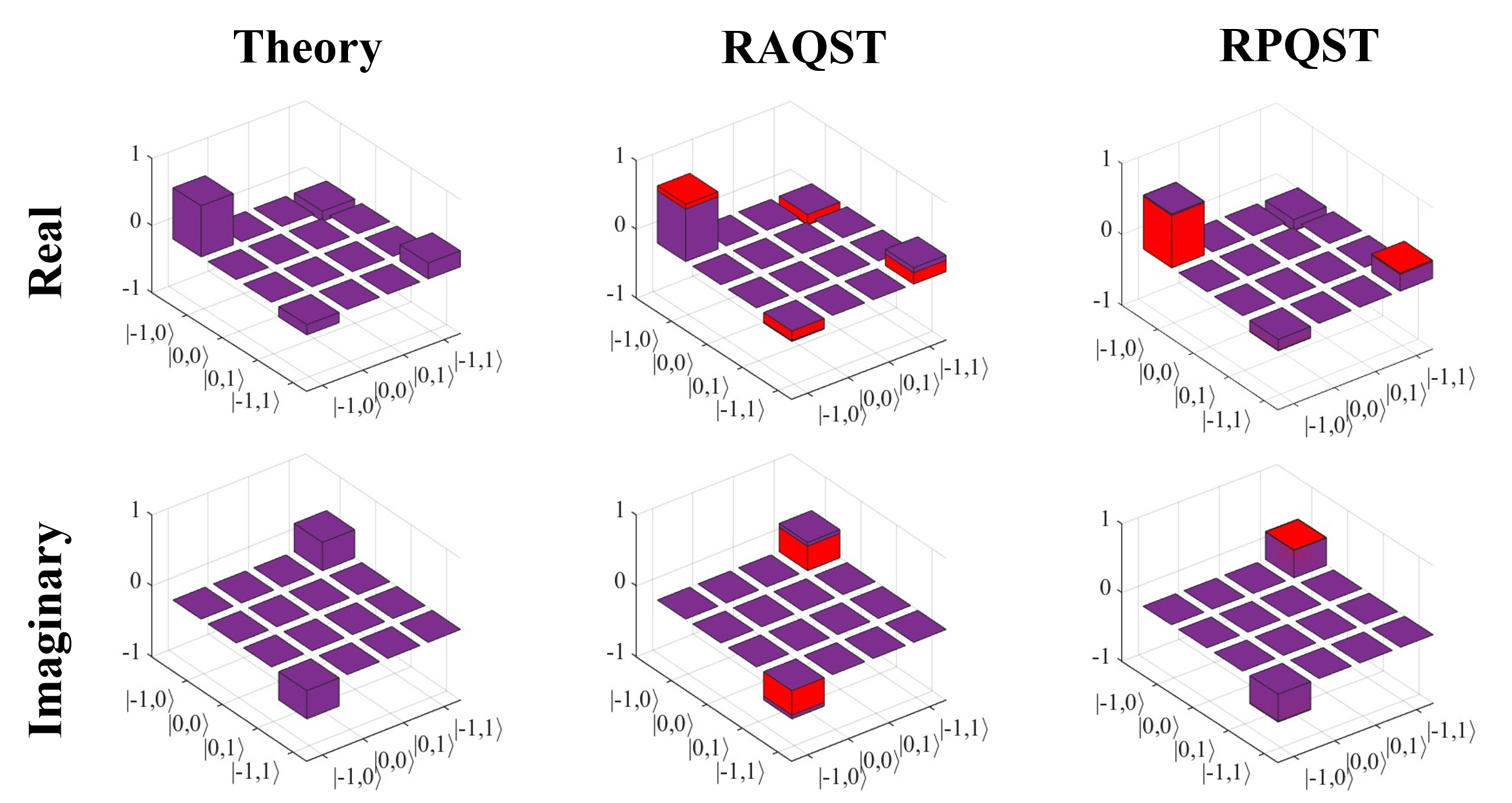
Figure 7: Real and imaginary parts of the expected density operator (Theory), for which the corresponding state parameters are ($\theta=58.41^{\circ}$ and $\phi=249^{\circ}$) and we have obtained the best fidelity, i.e. 0.9995. We also show the experimentally observed density matrices using method RAQST and method RPQST and compare them with the theoretical ideal. For this, in the last two columns, theoretical density matrix elements are plotted in purple and experimental ones in red. When the experimentally obtained values are larger, the bars are shown as purple with red on top (as on the bottom right). Vice versa, the bars are shown as red with purple on top (as in the middle figure of the bottom row).

The RAQST and RPQST measurements were performed for two other states. The error $\Delta$ on the measured angles $\theta$ and $\phi$ as well as fidelity $F$ for all three states are shown in the table:

	($58^{\circ},249^{\circ}$)	($137^{\circ},53^{\circ}$)	($88^{\circ},270^{\circ}$)
$(\Delta\theta,\Delta\phi)_{A}$	($8^{\circ},7^{\circ}$)	($4^{\circ},13^{\circ}$)	($12^{\circ},10^{\circ}$)
$F_{A}$	0.9919	0.9935	0.9806
$(\Delta\theta,\Delta\phi)_{P}$	($3^{\circ},1^{\circ}$)	($0^{\circ},10^{\circ}$)	($6^{\circ},3^{\circ}$)
$F_{P}$	0.9995	0.9963	0.9962

V Conclusion and discussion

We have devised a novel method for QST with two variants RAQST and RPQST involving Rabi experiments. Our method not only involves simple experiments, but also RPQST reduces the number of experiments from 3ⁿ to 2ⁿ for an n-qubit size register, which greatly reduces experimental time contrary to standard methods. Even in the case of RAQST, the routine $\pi$-pulse calibration experiment can be used as the reference experiment and then the time complexity in RAQST also scales as 2ⁿ. We systematically obtain very high fidelities above 0.996 by RPQST in all experiments for two-qubit hybrid spin states, with the best being 0.9995, which shows our ability of quantum state engineering with an excellent control. Moreover, RPQST outperforms RAQST as it suppresses systematic experimental errors. Our work puts a step forward towards fault-tolerant quantum computation using the electron-nuclear (e-¹⁴N) spin hybrid system in diamond which will eventually place NV center-based solid state spin-qubit systems among the prestigious group of error correction viable quantum computing architectures. We believe that such a good control of our hybrid system will allow us to have high-quality single-qubit and two-qubit quantum gates. Though, we have demonstrated our new method for QST using ODMR, the work on photoelectric detection of magnetic resonance (PDMR)Bourgeois et al. (2020) QST is an ongoing venture. The PDMR-QST will be an unavoidable tool for achieving high-fidelity state engineering in a scalable dipole-dipole coupled NV spin register desirable for fault-tolerant programmable quantum computers. Further enhancement of fidelity is possible by characterising types of noises and systematic errors and suppressing the decoherence effect by using dynamical decoupling pulses. Moreover, we are working on numerically designed pulses using optimal control theory to get rid of systematic errors in the implementation. In addition, we are also improving the hardware for suppressing inhomogeneity in the microwave control field. We report our method, control techniques, and experimental results believing that it will be helpful for the NV center-based quantum information processing community for further improving the methods and in building quantum information processing applications using NV center hybrid system at room temperature.

References

- Arute et al. (2019) F. Arute, K. Arya, R. Babbush, D. Bacon, J. C. Bardin, R. Barends, R. Biswas, S. Boixo, F. G. Brandao, D. A. Buell, et al., Nature 574, 505 (2019).
- Zhong et al. (2020) H.-S. Zhong, H. Wang, Y.-H. Deng, M.-C. Chen, L.-C. Peng, Y.-H. Luo, J. Qin, D. Wu, X. Ding, Y. Hu, et al., Science 370, 1460 (2020).
- Ristè et al. (2017) D. Ristè, M. P. Da Silva, C. A. Ryan, A. W. Cross, A. D. Córcoles, J. A. Smolin, J. M. Gambetta, J. M. Chow, and B. R. Johnson, npj Quantum Information 3, 16 (2017).
- Morvan et al. (2023) A. Morvan, B. Villalonga, X. Mi, S. Mandra, A. Bengtsson, P. Klimov, Z. Chen, S. Hong, C. Erickson, I. Drozdov, et al., arXiv preprint arXiv:2304.11119 (2023).
- Andreas et al. (2021) B. Andreas, B. Guillaume, J. Binder, B. Thierry, H. Ehm, T. Ehmer, M. Erdmann, G. Norbert, H. Philipp, M. Hess, et al., EPJ Quantum Technology 8 (2021).
- Nielsen and Chuang (2010) M. A. Nielsen and I. L. Chuang, Quantum computation and quantum information (Cambridge university press, 2010).
- Stolze and Suter (2008) J. Stolze and D. Suter, Quantum computing: a short course from theory to experiment (John Wiley & Sons, 2008).
- Hanson et al. (2008) R. Hanson, V. Dobrovitski, A. Feiguin, O. Gywat, and D. Awschalom, Science 320, 352 (2008).
- Fehler et al. (2019) K. G. Fehler, A. P. Ovvyan, N. Gruhler, W. H. P. Pernice, and A. Kubanek, ACS Nano 13, 6891 (2019), pMID: 31184854, https://doi.org/10.1021/acsnano.9b01668 .
- Siyushev et al. (2019) P. Siyushev, M. Nesladek, E. Bourgeois, M. Gulka, J. Hruby, T. Yamamoto, M. Trupke, T. Teraji, J. Isoya, and F. Jelezko, Science 363, 728 (2019).
- Ruf et al. (2021) M. Ruf, N. H. Wan, H. Choi, D. Englund, and R. Hanson, Journal of Applied Physics 130 (2021).
- Chakraborty et al. (2017) T. Chakraborty, J. Zhang, and D. Suter, New Journal of Physics 19, 073030 (2017).
- Shukla et al. (2022) A. Shukla, B. Carmans, M. Petrov, and M. Nesladek, “Supplementary material for high fidelity quantum state tomography of 14N nuclear spin in diamond,” (2022).
- Bourgeois et al. (2020) E. Bourgeois, M. Gulka, and M. Nesladek, Advanced Optical Materials 8, 1902132 (2020).