Dimension-free comparison estimates for suprema of some canonical processes

Abstract

We obtain error approximation bounds between expected suprema of canonical processes that are generated by random vectors with independent coordinates and expected suprema of Gaussian processes. In particular, we obtain a sharper proximity estimate for Rademacher and Gaussian complexities. Our estimates are dimension-free, and depend only on the geometric parameters and the numerical complexity of the underlying index set.

2020 Mathematics Subject Classification. Primary: 60G15; Secondary: 68Q87.

Keywords and phrases. Rademacher complexity, Stein’s method, Sudakov minoration, Gibbs’ measures.

1 Introduction

Expected suprema of canonical processes play a very important role in geometric functional analysis and asymptotic convex geometry [AAGM15], and recently in high-dimensional statistics and machine learning [BM02], [RV08], [ALMT14], [TH15], [OT18]. On the other hand, even for most prototypical canonical processes (such as Gaussian and Rademacher processes), understanding their expected suprema could be a highly non-trivial endeavour [Tal87],[BL14]. Consequently, in many theoretical and practical studies, it is very useful to be able to compare expected suprema of different stochastic processes (without having to estimate them directly). In this paper, we study the class of canonical processes $\{\xi_{t}\}_{t\in T}$ of the form

$$\xi_{t}:=\langle\xi,t\rangle=\sum_{i=1}^{n}t_{i}\xi_{i},$$

where $\xi$ is a random vector on $\mathbb{R}^{n}$ with independent coordinates and $T\subset\mathbb{R}^{n}$ is finite. We are interested in the quantity $\mathbb{E}\sup_{t\in T}\xi_{t}$. More precisely, given a canonical process $\{\xi_{t}\}_{t\in T}$, we are interested in comparing its expected supremum $\mathbb{E}\sup_{t\in T}\xi$ with that of the canonical Gaussian process $\{\langle G,t\rangle\}_{t\in T}$ where $G=(g_{1},g_{2},\ldots,g_{n})$ is a standard Gaussian random vector on $\mathbb{R}^{n}$ (that is, $g_{i}$ are i.i.d. $\mathcal{N}(0,1)$ random variables for $1\leq i\leq n$).

In the Gaussian case, the expected behavior of the supremum of a process is very well understood and intimately tied to the geometry of the index set $(T,d)$, where $d$ is the usual Euclidean metric on $\mathbb{R}^{n}$, that is, $d(t,s):=\|t-s\|_{2}=(\sum_{i=1}^{n}|t_{i}-s_{i}|^{2})^{1/2}$. In fact, the celebrated Fernique-Talagrand majorizing measure theorem [Tal87] fully characterizes the expected supremum of a canonical Gaussian process in terms of the geometry of the underlying index set. We refer the reader to [Tal21, Chapter 2], [Tal01], and [Tal96] for a more general and thorough analysis on suprema of Gaussian processes.

Given that we understand the class of canonical Gaussian processes very well, the main idea is to establish a comparison principle between the expected supremum of a canonical Gaussian process and expected supremum of a canonical process that one wish to understand, thereby leveraging the rich theory already developed about canonical Gaussian processes to gain insights into the behavior of expected suprema of other stochastic processes.

These ideas were used by Talagrand in [Tal02] in studying universality in Sherrington-Kirkpatrick (SK) model, a very important model in the theory of Spin glasses [Tal03], [CH06]. Chatterjee in [Cha05] also used a similar idea for studying error bound in Sudakov-Fernique inequality. Before moving further, let us introduce some notation:

(1.1) $$g(T):=\mathbb{E}\sup_{t\in T}\langle G,t\rangle$$

and is called the Gaussian complexity of the set $T$. A random vector on $\mathbb{R}^{n}$ with i.i.d. Rademacher (symmetric Bernoulli) coordinates $\epsilon_{i}$ is denoted by $\mathcal{E}=(\epsilon_{1},\epsilon_{2},\ldots,\epsilon_{n})$. Let $\mathcal{E}_{t}:=\langle\mathcal{E},t\rangle=\sum_{i=1}^{n}t_{i}\epsilon_{i}$   for $t\in T$. We define

(1.2) $$r(T):=\mathbb{E}\sup_{t\in T}\langle\mathcal{E},t\rangle$$

and is called the Rademacher complexity of the set $T$. Here and elsewhere, $C>0$ and $L>0$ denote universal constants, not necessarily the same at each occurrence.

The following comparison “principle" was proven by Talagrand in [Tal02]:

Theorem 1.1 (Talagrand).

Let $T\subset\mathbb{R}^{n}$ be finite, $R_{\infty}(T):=\sup_{t\in T}\|t\|_{\infty}$ , and $R_{2}(T):=\sup_{t\in T}\|t\|_{2}$ . Then, there exists an absolute constant C such that

$$\left|r(T)-g(T)\right|\leq C\sqrt{R_{2}R_{\infty}}(\log|T|)^{3/4}.$$

Analogous to the proof of lower bound for Gaussian complexity $g(T)$ in the majorizing measure theorem [Tal01], the proof of the lower bound for Rademacher complexity $r(T)$ in the Latala-Bednorz theorem is based on two fundamental facts, namely, the (sub-gaussian) concentration and the Sudakov minoration for Rademacher processes [BL14]. Having theorem 1.1 at our disposal, one can recover the Sudakov minoration for Rademacher processes :

Corollary 1.2 (Sudakov minoration for Rademacher process).

There exists a universal constant $C>0$ with the following property. Let $T\subset\mathbb{R}^{n}$ be finite and such that $\|u-v\|_{2}\geq a>0$ for all $u,v\in T$ whenever $u\neq v$, and let $R_{2}(T)=\sup_{t\in T}\|t\|_{2}$. Suppose that

$$\|t\|_{\infty}\leq Ca^{2}/(R_{2}\sqrt{\log|T|}),\quad\forall t\in T.$$

Then, we have

(1.3) $$r(T)\geq Ca\sqrt{\log|T|}.$$

Remark 1.3.

It is well known (see e.g., [Ver18, Chapter 2]) that due to sub-gaussian behavior one has $\left\lvert g(T)\right\rvert$, $\left\lvert r(T)\right\rvert$ $\leq$ $CR_{2}\sqrt{\log|T|},$ and so Theorem 1.1 is of interest only when its right-hand side is smaller than this quantity. That is, when $R_{\infty}\sqrt{\log|T|}\leq R_{2}$.

The above Theorem 1.1 together with Remark 1.3 can be intuitively understood as a consequence of the Central Limit Theorem: In general, tails of $\sum_{i=1}^{n}t_{i}\epsilon_{i}$ could be very different from the tails of $\sum_{i=1}^{n}t_{i}g_{i}$. However, when each of the components $t_{i}$ of $t$ is small compared to $\left\lVert t\right\rVert_{2}$ (that is, when $R_{\infty}\sqrt{\log|T|}\leq R_{2}$), then by the Central limit theorem, the random variable $\sum_{i=1}^{n}t_{i}\epsilon_{i}$ will resemble more like a Gaussian random variable.

With the above understanding, one can then look to generalize to other distributions. More precisely, one should expect tighter bounds for $\left\lvert\mathbb{E}\sup_{t\in T}\langle\xi,t\rangle-g(T)\right\rvert$ whenever the components $t_{i}$ of $t$ are small compared to $\left\lVert t\right\rVert_{2}$ and $R_{\infty}\sqrt{\log|T|}\leq R_{2}$ replaced by a similar condition depending on the distribution of $\xi$. This brings us to our contributions in this paper. First, let us introduce the following notation: For a random vector $\xi=(\xi_{1},\xi_{2},\ldots,\xi_{n})$ on $\mathbb{R}^{n}$, define

(1.4) $$c_{\xi}(T):=\mathbb{E}\sup_{t\in T}\langle\xi,t\rangle=\mathbb{E}\sup_{t\in T}\sum_{i=1}^{n}t_{i}\xi_{i}$$

for $t\in T$, where $T\subset\mathbb{R}^{n}$ is finite. The quantity $c_{\xi}(T)$ can be interpreted analogously as measuring geometrical complexity of $T$ with respect to the distribution of the random vector $\xi$.

In this paper, we derive upper estimates for the quantity $\left\lvert c_{\xi}(T)-g(T)\right\rvert$ under various relaxed assumptions (than Theorem 1.1) on the random vector $\xi$. More precisely:

• In Corollary 3.4, we derive upper estimates on $\left\lvert c_{\xi}(T)-g(T)\right\rvert$ under independence and mild moment assumptions on the coordinates of $\xi$, and no further distributional assumption on $\xi$.

• In Theorem 3.8, we generalize and sharpen Talagrand’s Theorem 1.1 by replacing $\sqrt{R_{2}R_{\infty}}$ with a sharper quantity $R_{4}(T):=\sup_{t\in T}\left\lVert t\right\rVert_{4}$.

• All our estimates for $\left\lvert c_{\xi}(T)-g(T)\right\rvert$ depend only on the geometric parameters and numerical complexity (namely, $\log|T|$) of the underlying index set $T$. This is in line with the popular anticipation that “size” of a “nearly” Gaussian process must be related with the geometry of the underlying metric space $(T,d)$ [Tal21, Chapter 1]. Importantly, there is no explicit dependence on the dimension $n$, and hence dimension-free in the title.
  

Our method of proof is inspired by Talagrand’s interpolation technique in [Tal02] wherein a clever hands-on interpolation is being used to compare $\sum_{i=1}^{n}t_{i}\epsilon_{i}$ with $\sum_{i=1}^{n}t_{i}g_{i}$ for $t\in T$. We use a similar idea based on Stein’s method by integrating tools from Ornstein-Uhlenbeck semigroup with the tools from theory of Spin glasses and Gibbs’ measures to construct a more natural and refined interpolation between $c_{\xi}(T)$ and $g(T)$. Thus, in particular, leading to a sharper estimate in terms of $R_{4}$ than in Theorem 1.1in [Tal02].

Rest of the paper is organized as follows:

• In Section 2 we provide necessary background material on Gibbs’ measures and Ornstein-Uhlenbeck semigroup (Stein’s method).

• In section 3 we present our advertised results (namely Corollary 3.4 and Theorem 3.8): We provide full proofs and discussions on various aspects of the proofs.

• Section 4: In sub-section 4.1, we provide a picture, figure 1, facilitating a visual comparison between our Theorem 3.8 and Talagrand’s Theorem 1.1. Additionally, in 4.1.1, we provide examples witnessing $R_{4}\ll\sqrt{R_{2}R_{\infty}}$ in the context of Theorem 3.8 and Talagrand’s Theorem 1.1. In sub-section 4.2.1, as an application of our results, we discuss universality for order-m tensors. In sub-section 4.2.2, we discuss generalizations of our results when the index set $T$ is equipped with an arbitrary probability measure $\mu$.

2 Background material

2.1 Smooth approximation and Gibbs’ measures

Let $\beta>0$ and $T\subset\mathbb{R}^{n}$ be finite. Recall the so-called log-partition function $F_{\beta}$ defined by

$$F_{\beta}(x)=\frac{1}{\beta}\log\left(\sum_{t\in T}e^{\beta\langle x,t\rangle}\right).$$

Partial differentiation with respect to $x_{i}$ yields

(2.1) $$\partial_{i}F_{\beta}(x)=\frac{\sum_{t\in T}e^{\beta\langle x,t\rangle}t_{i}}{\sum_{t\in T}e^{\beta\langle x,t\rangle}}.$$

If we consider the probability measures (called Gibbs’ measures in statistical physics; cf. [Bar16] for applications in discrete mathematics) $\left\{\mu_{x}\mid x\in\mathbb{R}^{n}\right\}$ on $T$ assigning mass

(2.2) $$\mu_{x}(\{t\})=\frac{e^{\beta\langle x,t\rangle}}{\sum_{t\in T}e^{\beta\langle x,t\rangle}},\quad t\in T,$$

then the latter derivative can be expressed as an expectation with respect to this measure, that is,

(2.3) $$\partial_{i}F_{\beta}(x)=\mathbb{E}_{\mu_{x}}[\ell_{i}],\quad\ell_{i}(t)=\langle t,e_{i}\rangle=t_{i}.$$

We have the following:

Lemma 2.1 (Properties of $F_{\beta}$).

Let $T\subset\mathbb{R}^{n}$ be a finite set and let $\beta>0$. Then, we have the following properties:

1. $F_{\beta}$ is convex.

2. $F_{\beta}$ is Lipschitz. For all $x$ we have

   $$\|\nabla F_{\beta}(x)\|_{2}\leq R_{2}(T).$$

3. For all $x\in\mathbb{R}^{n}$ one has

   (2.4) $$\max_{t\in T}\langle x,t\rangle\leq F_{\beta}(x)\leq\max_{t\in T}\langle x,t\rangle+\frac{\log|T|}{\beta}.$$

Proof.

1. The 2nd order partial derivatives of $F_{\beta}$ are given by

   $$\partial_{ij}F_{\beta}(x)=\mathbb{E}_{\mu_{x}}[\ell_{i}\ell_{j}]-\mathbb{E}_{\mu_{x}}[\ell_{i}]\cdot\mathbb{E}_{\mu_{x}}[\ell_{j}]=[{\rm Cov}(\ell_{i},\ell_{j})]_{\mu_{x}}.$$

2. Let $\|u\|_{2}=1$. Then, we may write

   $$\langle\nabla F_{\beta}(x),u\rangle=\sum_{i}u_{i}\partial_{i}F_{\beta}(x)=\mathbb{E}_{\mu_{x}}[\langle\cdot,u\rangle]\leq\max_{t\in T}\langle t,u\rangle\leq R_{2}(T),$$

   Since $u$ was arbitrary the result follows.

3. Since $\beta>0$, we may write

   $$\exp\left(\beta\max_{t\in T}\langle x,t\rangle\right)\leq\sum_{t\in T}e^{\beta\langle x,t\rangle}\leq|T|e^{\beta\max_{t\in T}\langle x,t\rangle}.$$

   Applying logarithm and dividing by $\beta$ gives the result. $\hfill\quad\Box$
   

Lemma 2.2 (Bounds for higher derivatives of $F_{\beta}$).

Let $T\subset\mathbb{R}^{n}$ be finite and let $F_{\beta}$ as above. Then, for all $x\in\mathbb{R}^{n}$ we have the following bounds:

(2.5) $$|\partial_{i}^{(3)}F_{\beta}(x)|\leq 6\beta^{2}\mathbb{E}_{\mu_{x}}[|\ell_{i}|^{3}],\quad|\partial_{i}^{(4)}F_{\beta}(x)|\leq 26\beta^{3}\mathbb{E}_{\mu_{x}}[\ell_{i}^{4}].$$

In particular,

(2.6) $$|\partial_{i}^{(3)}F_{\beta}(x)|\leq 6\beta^{2}\max_{t\in T}|t_{i}|^{3},\quad|\partial_{i}^{(4)}F_{\beta}(x)|\leq 26\beta^{3}\max_{t\in T}|t_{i}|^{4}.$$

Proof. It is straightforward to check that

$$\partial_{i}^{(2)}F_{\beta}(x)=\beta{\rm Var}_{\mu_{x}}[\ell_{i}].$$

Similarly, we get

$$\partial_{i}^{(3)}F_{\beta}(x)=\beta^{2}\mathbb{E}_{\mu_{x}}[\ell_{i}^{3}]-3\beta^{2}\mathbb{E}_{\mu_{x}}[\ell_{i}]\cdot\mathbb{E}_{\mu_{x}}[\ell_{i}^{2}]+2\beta^{2}\left(\mathbb{E}_{\mu_{x}}[\ell_{i}]\right)^{3}=\beta^{2}\mathbb{E}_{\mu_{x}}\left[(\ell_{i}-\mathbb{E}_{\mu_{x}}[\ell_{i}])^{3}\right],$$

and

$$\partial_{i}^{(4)}F_{\beta}(x) =\beta^{3}\mathbb{E}_{\mu_{x}}[\ell_{i}^{4}]-4\beta^{3}\mathbb{E}_{\mu_{x}}[\ell_{i}^{3}]\cdot\mathbb{E}_{\mu_{x}}[\ell_{i}]-3\beta^{3}\left(\mathbb{E}_{\mu_{x}}[\ell_{i}^{2}]\right)^{2}+12\beta^{3}\left(\mathbb{E}_{\mu_{x}}[\ell_{i}]\right)^{2}\cdot\mathbb{E}_{\mu_{x}}[\ell_{i}^{2}]-6\beta^{3}\left(\mathbb{E}_{\mu_{x}}[\ell_{i}]\right)^{4}$$

$$=\beta^{3}\mathbb{E}_{\mu_{x}}\left[(\ell_{i}-\mathbb{E}_{\mu_{x}}[\ell_{i}])^{4}\right]-3\beta^{3}\left({\rm Var}_{\mu_{x}}[\ell_{i}]\right)^{2}.$$

Therefore, triangle inequality and Hölder’s inequality yield

$$|\partial_{i}^{(3)}F_{\beta}(x)| \leq 6\beta^{2}\mathbb{E}_{\mu_{x}}[|\ell_{i}|^{3}],$$

and

$$|\partial_{i}^{(4)}F_{\beta}(x)| \leq 26\beta^{3}\mathbb{E}_{\mu_{x}}[\ell_{i}^{4}],$$

as desired.

The “in particular” case follows from the simple fact that $\mathbb{E}_{\mu_{x}}\left[\left\lvert f\right\rvert\right]\leq\max_{t\in T}|f(t)|$. $\hfill\quad\Box$

2.2 Stein’s method

Consider the distance between probability distributions $\mu$ and $\mu_{0}$ on $\mathbb{R}^{n}$ of the form

(2.7) $$d_{{\cal H}}(\mu,\mu_{0}):=\sup_{h\in\mathcal{H}}|\mathbb{E}_{\mu}h-\mathbb{E}_{\mu_{0}}h|,$$

where $\mathcal{H}$ is a set of test functions. Such distances are called integral probability metrics. As described in [Cha14], one of the goals of Stein’s method is to obtain explicit bounds on the distance between a probability distribution $\mu$ of interest and a usually very well-understood approximating distribution $\mu_{0}$, often called the target distribution. A test function $h$ is connected to the distribution of interest through a Stein Equation

(2.8) $$h(x)-\mathbb{E}_{\mu_{0}}h=\mathcal{T}f(x),$$

where $\mathcal{T}$ is a Stein’s operator for the distribution $\mu_{0}$ along with an associated Stein’s class $\mathcal{T(F)}$ of functions such that

$$\mathbb{E}_{\mu_{0}}[\mathcal{T}f(Z)]=0\quad\text{for all}\quad f\in\mathcal{T(F)}\quad\iff\quad Z\sim\mu_{0}.$$

Hence the distance (2.7) can be bounded using

$$d_{\mathcal{H}}(\mu,\mu_{0})\leq\sup_{f\in\mathcal{F}(\mathcal{H})}|\mathbb{E}_{\mu}\mathcal{T}f(X)|,$$

where $\mathcal{F}(\mathcal{H})=\{f_{h}\mid h\in\mathcal{H}\}$ is the set of solutions of the Stein equation (2.8) for the test functions $h\in\mathcal{H}$.

For a more in depth and comprehensive understanding of Stein’s method, we refer the reader to [Ste72], [CGS11], and [Cha14]. Since the basic ingredient for materializing the normal (Gaussian) approximation in the Stein’s method is Ornstein-Uhlenbeck (OU) semigroup [BGL14], we next recall some of the important definitions and results in this context:

2.2.1 Ornstein–Uhlenbeck (OU) semigroup

Definition 2.3 (OU semigroup).

Let $P_{t}:L^{1}(\gamma_{n})\to L^{1}(\gamma_{n})$ be defined by

(2.9) $$(P_{t}f)(x):=\mathbb{E}f(e^{-t}x+\sqrt{1-e^{-2t}}G),$$

where $\enspace t\geq 0$, $\enspace G\sim N({\bf 0},I_{n})$, and $\,\gamma_{n}$ is the standard Gaussian measure on $\mathbb{R}^{n}$.

The generator $L$ associated with the semigroup $P_{t}$, that is, $Lf=\lim_{t\to 0^{+}}\frac{P_{t}f-f}{t}$ is given by

$$Lu(x)=\Delta u(x)-\langle x,\nabla u(x)\rangle$$

for $u\in C^{2}$. It is known that $P_{t}f$ solves the following boundary value problem:

$$\begin{cases}Lu(x,t)=\partial_{t}u(x,t)\\ u(x,0)=f(x).\end{cases}$$

We also define (formally) the following operator:

(2.10) $$({\mathscr{P}}f)(x):=\int_{0}^{\infty}\left(P_{t}f(x)-\mathbb{E}f(G)\right)\,dt,\quad x\in\mathbb{R}^{n}.$$

Note that the right-hand side converges for Lipschitz maps $f$. Indeed;

$$|P_{t}f(x)-\mathbb{E}[f(G)]| =|\mathbb{E}[f(e^{-t}x+\sqrt{1-e^{-2t}}G)-f(G)]|$$

$$\leq\|f\|_{\rm Lip}\mathbb{E}\left\|e^{-t}x-\frac{e^{-2t}}{1+\sqrt{1-e^{-2t}}}G\right\|$$

$$\leq e^{-t}\|f\|_{\rm Lip}\left(\|x\|+\mathbb{E}\|G\|\right).$$

Given $f\in L^{1}(\gamma_{n})$ and $x\in\mathbb{R}^{n}$, we may write

(2.11) $$f(x)-\mathbb{E}f(G) =-\int_{0}^{\infty}\frac{d}{dt}P_{t}f(x)\,dt=-\int_{0}^{\infty}LP_{t}f(x)\,=-{\mathscr{P}}Lf(x)=-L{\mathscr{P}}f(x),$$

where the last equality follows from the dominated convergence theorem.

Also, recall that

(2.12) $$\partial_{i}^{(k)}{\mathscr{P}}f(x)=\int_{0}^{\infty}e^{-tk}P_{t}(\partial_{i}^{(k)}f)(x)\,dt.$$

For proofs of (2.11) and (2.12), and for other details with respect to Ornstein-Uhlenbeck (OU) semigroup, we refer the reader to [BGL14, Chapter 1].

3 Main Results

Lemma 3.1.

Let $\xi=(\xi_{1},\ldots,\xi_{n})$ be a random vector with independent coordinates, with $\mathbb{E}\xi_{i}=0$ and $\mathbb{E}\xi_{i}^{2}=1$. We have the following formulae:

1. If $\mathbb{E}|\xi_{i}|^{3}<\infty$ for all $i\leq n$, then for any $C^{3}$-smooth function $f:\mathbb{R}^{n}\to\mathbb{R}$ we have

   (3.1) $$\mathbb{E}\left[Lf(\xi)\right]=\sum_{i=1}^{n}\mathbb{E}\left[\xi_{i}\int_{0}^{1}\partial_{i}^{(3)}f(\xi^{(i)}+s\xi_{i}e_{i})\,ds\right]-\sum_{i=1}^{n}\mathbb{E}\left[\xi_{i}^{3}\int_{0}^{1}(1-s)\partial_{i}^{(3)}f(\xi^{(i)}+s\xi_{i}e_{i})\,ds\right].$$

2. If, additionally, $\mathbb{E}\xi_{i}^{3}=0$ and $\mathbb{E}\xi_{i}^{4}<\infty$ for all $i\leq n$, then for any $C^{4}$-smooth function $f:\mathbb{R}^{n}\to\mathbb{R}$ we have

   (3.2) $$\begin{split}\mathbb{E}\left[Lf(\xi)\right]=\sum_{i=1}^{n}\mathbb{E}\left[\xi_{i}^{2}\int_{0}^{1}(1-s)\partial_{i}^{(4)}f(\xi^{(i)}+s\xi_{i}e_{i})\,ds\right]-\sum_{i=1}^{n}\mathbb{E}\left[\frac{\xi_{i}^{4}}{2}\int_{0}^{1}(1-s)^{2}\partial_{i}^{(4)}f(\xi^{(i)}+s\xi_{i}e_{i})\,ds\right].\end{split}$$

Proof. We shall demonstrate the proof of (3.2). We work similarly for (3.1). Recall that $L$ acts as follows:

(3.3) $$Lf(\xi)=\Delta f(\xi)-\sum_{i=1}^{n}\xi_{i}\partial_{i}f(\xi).$$

Using Taylor’s approximation theorem for $\partial_{i}f(\xi)$, and writing $\xi^{(i)}$ for $\xi-\xi_{i}e_{i}$, we get

$$\partial_{i}f(\xi)-\partial_{i}f(\xi^{(i)})=\xi_{i}\partial^{(2)}_{i}f(\xi^{(i)})+\xi^{2}_{i}\frac{1}{2}\partial^{(3)}_{i}f(\xi^{(i)})+\frac{1}{2!}\int_{0}^{\xi_{i}}(\xi_{i}-s)^{2}\partial_{i}^{(4)}f(\xi^{(i)}+se_{i})ds.$$

Using the substitution $s\to s\xi_{i}$, and multiplying both sides by $\xi_{i}$, we derive

$$\xi_{i}(\partial_{i}f(\xi)-\partial_{i}f(\xi^{(i)}))=\xi_{i}^{2}\partial_{i}^{(2)}f(\xi^{(i)})+\frac{\xi_{i}^{3}}{2}\partial_{i}^{(3)}f(\xi^{(i)})+\frac{\xi_{i}^{4}}{2}\int_{0}^{1}(1-s)^{2}\partial_{i}^{(4)}f(\xi^{(i)}+s\xi_{i}e_{i})\,ds.$$

Now using (3.3), we may write

$$Lf(\xi)=\Delta f(\xi)-\sum_{i=1}^{n}\xi_{i}(\partial_{i}f(\xi)-\partial_{i}f(\xi^{(i)}))-\sum_{i=1}^{n}\xi_{i}\partial_{i}f(\xi^{(i)}).$$

Taking expectations on both sides, and using the fact that $\xi_{i}$ are independent and satisfy the assumptions of (2), we obtain

(3.4) $$\mathbb{E}[Lf(\xi)]=\mathbb{E}\left[\hskip 2.84526pt\sum_{i=1}^{n}(\partial_{i}^{(2)}f(\xi)-\partial_{i}^{(2)}f(\xi^{(i)}))-\frac{1}{2}\sum_{i=1}^{n}\xi_{i}^{4}\int_{0}^{1}(1-s)^{2}\partial_{i}^{(4)}f(\xi^{(i)}+s\xi_{i}e_{i})\,ds\right].$$

Notice that using the Taylor’s approximation theorem for $\partial_{i}^{(2)}f(\xi)$, we obtain

$$\partial_{i}^{(2)}f(\xi)-\partial_{i}^{(2)}f(\xi^{(i)})=\xi_{i}\partial_{i}^{(3)}f(\xi^{(i)})+\int_{0}^{\xi_{i}}(\xi_{i}-s)\partial_{i}^{(4)}f(\xi^{(i)}+se_{i})\,ds.$$

Plugging this into (3.4), we get

$$\mathbb{E}[Lf(\xi)] =\sum_{i=1}^{n}\mathbb{E}\left[\xi_{i}^{2}\int_{0}^{1}(1-s)\partial_{i}^{(4)}f(\xi^{(i)}+s\xi_{i}e_{i})\,ds-\frac{\xi_{i}^{4}}{2}\int_{0}^{1}(1-s)^{2}\partial_{i}^{(4)}f(\xi^{(i)}+s\xi_{i}e_{i})\,ds\right],$$

as claimed. The proof is complete. $\hfill\quad\Box$

Remark 3.2.

We note in passing that one could use Lemma 3.1 to derive universality properties for various problems in communications, statistical learning, and random matrix theory by choosing the function $f$ in Lemma 3.1 appropriately as in [KM11].

Using the integral representation in Lemma 3.1 we may already get a (weaker) error approximation bound. Namely, this bound will depend on the following (geometric) parameter associated with the set $T$,

$$\|(e_{1},\ldots,e_{n})\|_{\ell_{p}(T)}:=\left(\sum_{i=1}^{n}\max_{t\in T}|\langle t,e_{i}\rangle|^{p}\right)^{1/p},$$

for $p=3$ or $p=4$ according to as employing (3.1) or (3.2). Namely, we have the following:

Proposition 3.3.

Let $T$ be a bounded subset of $\mathbb{R}^{n}$. Let $\xi=(\xi_{1},\ldots,\xi_{n})$ be a random vector with independent coordinates such that $\mathbb{E}\xi_{i}=0$ and $\mathbb{E}\xi_{i}^{2}=1$. We have the following cases:

1. If $\sigma_{3}^{3}:=\max_{i\leq n}\mathbb{E}|\xi_{i}|^{3}<\infty$, then for all $\beta>0$ we have

   (3.5) $$|\mathbb{E}F_{\beta}(\xi)-\mathbb{E}F_{\beta}(G)|\leq C\beta^{2}\sigma_{3}^{3}\|(e_{1},\ldots,e_{n})\|_{\ell_{3}(T)}^{3}.$$

2. Furthermore, if $\mathbb{E}\xi_{i}^{3}=0$ for all $i\leq n$ and $\sigma_{4}^{4}:=\max_{i\leq n}\mathbb{E}\xi_{i}^{4}<\infty$, then, for all $\beta>0$ we have

   (3.6) $$|\mathbb{E}F_{\beta}(\xi)-\mathbb{E}F_{\beta}(G)|\leq C\beta^{3}\sigma_{4}^{4}\|(e_{1},\ldots,e_{n})\|_{\ell_{4}(T)}^{4},$$

   where $C>0$ is a universal constant.

Proof. Using Stein’s method we may write as follows:

$$\mathbb{E}F_{\beta}(\xi)-\mathbb{E}F_{\beta}(G)=-\mathbb{E}_{\xi}\left[{\mathscr{P}}LF_{\beta}(\xi)\right]=-\mathbb{E}_{\xi}\left[L{\mathscr{P}}F_{\beta}(\xi)\right].$$

Applying Lemma 3.1 for “$f={\mathscr{P}}F_{\beta}$”, we infer

(3.7) $$\begin{split}\mathbb{E}F_{\beta}(\xi)-\mathbb{E}F_{\beta}(G)=-\sum_{i=1}^{n}\mathbb{E}\left[\xi_{i}^{2}\int_{0}^{1}(1-s)\partial_{i}^{(4)}{\mathscr{P}}F_{\beta}(\xi^{(i)}+s\xi_{i}e_{i})\,ds\right]+\sum_{i=1}^{n}\mathbb{E}\left[\frac{\xi_{i}^{4}}{2}\int_{0}^{1}(1-s)^{2}\partial_{i}^{(4)}{\mathscr{P}}F_{\beta}(\xi^{(i)}+s\xi_{i}e_{i})\,ds\right].\end{split}$$

In view of (2.12) we have

(3.8) $$\partial_{i}^{(4)}{\mathscr{P}}F_{\beta}(\xi^{(i)}+s\xi_{i}e_{i})=\int_{0}^{\infty}e^{-4t}P_{t}(\partial_{i}^{(4)}F_{\beta})(\xi^{(i)}+s\xi_{i}e_{i})\,dt.$$

Note that

(3.9) $$P_{t}(\partial_{i}^{(4)}F_{\beta})(\xi^{(i)}+s\xi_{i}e_{i})=\mathbb{E}_{g}\left[\partial_{i}^{(4)}F_{\beta}\left(e^{-t}(\xi^{(i)}+s\xi_{i}e_{i})+\sqrt{1-e^{-2t}}g\right)\right].$$

From Lemma 2.2 we conclude that

(3.10) $$|\partial_{i}^{(4)}F_{\beta}\left(e^{-t}(\xi^{(i)}+s\xi_{i}e_{i})+\sqrt{1-e^{-2t}}g\right)|\leq 26\beta^{3}\max_{t\in T}|t_{i}|^{4},$$

a.s. Therefore, combining the latter pointwise estimate with all the above we infer that

(3.11) $$\left|\mathbb{E}F_{\beta}(\xi)-\mathbb{E}F_{\beta}(G)\right|\leq\frac{26\beta^{3}}{4}\sum_{i=1}^{n}\mathbb{E}\xi_{i}^{2}\max_{t\in T}|t_{i}|^{4}+\frac{26\beta^{3}}{8}\sum_{i=1}^{n}\mathbb{E}\xi_{i}^{4}\max_{t\in T}|t_{i}|^{4}\leq\frac{39\beta^{3}}{4}\sigma_{4}^{4}\sum_{i=1}^{n}\max_{t\in T}|t_{i}|^{4}.$$

The proof is complete. $\hfill\quad\Box$

Corollary 3.4.

Let $T$ be a finite subset of $\mathbb{R}^{n}$ and let $\xi=(\xi_{1},\ldots,\xi_{n})$ be a random vector with independent coordinates such that $\mathbb{E}\xi_{i}=0$ and $\mathbb{E}\xi^{2}=1$ for all $i\leq n$. We have the following assertions:

1. If $\sigma_{3}^{3}:=\max_{i\leq n}\mathbb{E}|\xi_{i}|^{3}<\infty$, then

   (3.12) $$\left|\mathbb{E}\sup_{t\in T}\langle\xi,t\rangle-g(T)\right|\leq C\sigma_{3}\|(e_{i})_{i\leq n}\|_{\ell_{3}(T)}(\log|T|)^{2/3}.$$

2. Moreover, if $\mathbb{E}\xi_{i}^{3}=0$ and $\sigma_{4}^{4}:=\max_{i\leq n}\mathbb{E}|\xi_{i}|^{4}<\infty$, then

   (3.13) $$\left|\mathbb{E}\sup_{t\in T}\langle\xi,t\rangle-g(T)\right|\leq C\sigma_{4}\|(e_{i})_{i\leq n}\|_{\ell_{4}(T)}(\log|T|)^{3/4},$$

where $C>0$ is a universal constant.

Proof. We only prove (2): By virtue of Lemma 2.1 we have

$$\left|\mathbb{E}\sup_{t\in T}\langle\xi,t\rangle-g(T)\right|\leq\frac{\log|T|}{\beta}+\left|\mathbb{E}F_{\beta}(\xi)-\mathbb{E}F_{\beta}(G)\right|.$$

Invoking Proposition 3.3 we obtain

$$\left|\mathbb{E}\sup_{t\in T}\langle\xi,t\rangle-g(T)\right|\leq\frac{\log|T|}{\beta}+C\beta^{3}\sigma_{4}^{4}\|(e_{i})_{i}\|_{\ell_{4}(T)}^{4},$$

for all $\beta>0$. We optimize with respect to $\beta$ by choosing $\beta=\frac{(\log|T|)^{1/4}}{\sigma_{4}\ell_{4}(T)}$ . $\hfill\quad\Box$

For establishing the announced (stronger) error approximation bound in terms of $R_{4}(T)$, we assume additionally that the random variables are uniformly bounded. Under this assumption one may bound in a more efficient way the $\mathbb{E}_{\mu_{x}}[\ell_{i}^{4}]$, and thereby the $|\partial^{(4)}F_{\beta}(x)|$. Toward this end, we shall need the following technical result which also appeared in [Tal02]. Since its proof is short we reproduce it here for reader’s convenience.

Lemma 3.5.

Let $T\subset\mathbb{R}^{n}$ be bounded and let $\beta>0$. For any $x=(x_{1},\ldots,x_{i},\ldots x_{n})\in\mathbb{R}^{n}$ and $x^{\prime}=(x_{1},\ldots,x_{i}^{\prime},\ldots,x_{n})$ we have

(3.14) $$\mathbb{E}_{\mu_{x}}[\ell_{i}^{4}]\leq e^{2\beta R_{\infty}|x_{i}-x_{i}^{\prime}|}\mathbb{E}_{\mu_{x^{\prime}}}[\ell_{i}^{4}].$$

Proof. Let $\psi(x)=\mathbb{E}_{\mu_{x}}[\ell_{i}^{4}]$. Applying the Fundamental Theorem of Calculus we obtain

$$\log\psi(x)-\log\psi(x^{\prime})=\int_{x_{i}^{\prime}}^{x_{i}}(\partial_{i}\log\psi)(x^{(i)}+se_{i})\,ds,$$

where $x^{(i)}=(x_{1},\ldots,x_{i-1},0,x_{i+1},\ldots,x_{n})$. On the other hand

$$\partial_{i}\psi(z)=\beta\mathbb{E}_{\mu_{z}}[\ell_{i}^{5}]-\beta\mathbb{E}_{\mu_{z}}[\ell_{i}^{4}]\cdot\mathbb{E}_{\mu_{z}}[\ell_{i}],$$

for all $z$. Thereby, we get

$$|\partial_{i}\psi(z)|\leq 2\beta R_{\infty}\mathbb{E}_{\mu_{z}}[\ell_{i}^{4}]=2\beta R_{\infty}\psi(z).$$

Combing the latter estimate with the identity the result follows. $\hfill\quad\Box$

The next result is the counterpart of Proposition 3.3 in the case of uniformly bounded random variables. More precisely, we have the following:

Proposition 3.6.

Let $T\subset\mathbb{R}^{n}$ be bounded and let $\beta>0$. Then, for any random vector $\xi=(\xi_{1},\ldots,\xi_{n})$ with independent coordinates, where $\mathbb{E}\xi_{i}=\mathbb{E}\xi_{i}^{3}=0$, $\mathbb{E}\xi_{i}^{2}=1$ and $|\xi_{i}|\leq M$ a.s. for all $i\leq n$, we have that

(3.15) $$\left|\mathbb{E}F_{\beta}(\xi)-\mathbb{E}F_{\beta}(G)\right|\leq 4\beta^{3}M^{4}R_{4}^{4}e^{2\beta MR_{\infty}}.$$

Proof. The first half of the argument is the same as in Proposition 3.3. It starts differentiating at the point where we bound $|\partial_{i}^{(4)}F_{\beta}(\cdot)|$. Recall that Lemma 2.2 yields the (pointwise) bound

(3.16) $$\left|\partial_{i}^{(4)}F_{\beta}\left(e^{-t}(\xi^{(i)}+s\xi_{i}e_{i})+\sqrt{1-e^{-2t}}g\right)\right|\leq 26\beta^{3}\mathbb{E}_{\mu_{z_{i}}}[\ell_{i}^{4}],$$

a.s., where $z_{i}=e^{-t}(\xi^{(i)}+s\xi_{i}e_{i})+\sqrt{1-e^{-2t}}g$. If we set $z=e^{-t}\xi+\sqrt{1-e^{-2t}}g$, an appeal to Lemma 3.5 (applied for “$x^{\prime}=z$” and “$x=z_{i}$”) yields the (almost sure) bound

(3.17) $$\mathbb{E}_{\mu_{z_{i}}}[\ell_{i}^{4}]\leq e^{2\beta(1-s)R_{\infty}e^{-t}|\xi_{i}|}\mathbb{E}_{\mu_{z}}[\ell_{i}^{4}]\leq e^{2\beta MR_{\infty}}\mathbb{E}_{\mu_{z}}[\ell_{i}^{4}].$$

Thus, (3.16) and (3.17) imply that

(3.18) $$\left|\partial_{i}^{(4)}F_{\beta}\left(e^{-t}(\xi^{(i)}+s\xi_{i}e_{i})+\sqrt{1-e^{-2t}}g\right)\right|\leq 26\beta^{3}e^{2\beta MR_{\infty}}\mathbb{E}_{\mu_{z}}[\ell_{i}^{4}],$$

for all $\xi$, and for all $0\leq s\leq 1$ and $t\geq 0$. Taking into account (3.8), (3.9), and (3.18) we obtain

(3.19) $$|\partial_{i}^{(4)}{\mathscr{P}}F_{\beta}(\xi^{(i)}+\tau\xi_{i}e_{i})|\leq 26\beta^{3}e^{2\beta MR_{\infty}}\int_{0}^{\infty}e^{-4s}\mathbb{E}_{g}\mathbb{E}_{\mu_{e^{-s}\xi+\sqrt{1-e^{-2s}}g}}[\ell_{i}^{4}]\,ds.$$

Finally, combining (3.19) with (3.7) we obtain

$$\left|\mathbb{E}F_{\beta}(\xi)-\mathbb{E}F_{\beta}(G)\right| \leq 26\beta^{3}M^{3}e^{2\beta MR_{\infty}}\int_{0}^{1}(1-\tau)\left(\int_{0}^{\infty}e^{-4s}\mathbb{E}_{g}\mathbb{E}_{\mu_{e^{-s}\xi+\sqrt{1-e^{-2s}}g}}[\|t\|_{4}^{4}]\,ds\right)\,d\tau$$

$$\hfill+\frac{26\beta^{3}}{2}M^{4}e^{2\beta MR_{\infty}}\int_{0}^{1}(1-\tau)^{2}\left(\int_{0}^{\infty}e^{-4s}\mathbb{E}_{\xi,g}\mathbb{E}_{\mu_{e^{-s}\xi+\sqrt{1-e^{-2s}}g}}[\|t\|_{4}^{4}]\,ds\right)\,d\tau$$

$$\leq\frac{27}{4}\beta^{3}M^{4}R_{4}^{4}e^{2\beta MR_{\infty}},$$

where we have used the fact that $M\geq(\mathbb{E}\xi_{i}^{2})^{1/2}=1$. The proof is complete. $\hfill\quad\Box$

Remark 3.7.

In estimate (3.17), instead of using Lemma 3.5, one might hope to show that there is a “majorant" probability measure $\nu$ (independent of $i$) on $T$ such that

$$\mathbb{E}_{\mu_{z_{i}}}[\ell_{i}^{4}]\leq C\,\mathbb{E}_{\nu}[\ell_{i}^{4}]$$

for all $i\in\{1,2,\ldots,n\}$ and for some universal constant $C>0$, thereby implying that

(3.20) $$\sum_{i=1}^{n}\mathbb{E}_{\mu_{z_{i}}}[\ell_{i}^{4}]\leq\sum_{i=1}^{n}C\,\mathbb{E}_{\nu}[\ell_{i}^{4}]\leq C\,R_{4}^{4},$$

and hence sharpening Proposition 3.6 (by removing exponential dependence on $R_{\infty}$). We next show that such a “majorant" measure $\nu$ does not exist in general.

First notice that in estimate (3.17), one may assume without loss of generality that $z_{i}=\xi^{(i)}+s\xi_{i}e_{i}$. Also, we see that in (3.20), right-hand side does not depend on $\xi$, or $\beta>0$ and $s\in[0,1]$. For $\theta>0$, consider the set $T_{\theta}=\big{\{}-\theta e_{j}\,|\,1\leq j\leq n\}$, where $\{e_{j}\}_{j=1}^{n}$ is the canonical basis in $\mathbb{R}^{n},$ and assume $\xi_{i}$ are $i.i.d.$ Rademacher random variables . We get

$$\mathbb{E}_{\mu_{\xi^{(i)}+s\xi_{i}e_{i}}}[\ell_{i}^{4}] =\sum_{j=1}^{n}[\ell_{i}(-\theta e_{j})]^{4}\,\,\,\frac{e^{\beta\langle-\theta e_{j},\,\xi^{(i)}+s\xi_{i}e_{i}\rangle}}{\sum_{j=1}^{n}e^{\beta\langle-\theta e_{j},\,\xi^{(i)}+s\xi_{i}e_{i}\rangle}}$$

$$=\theta^{4}\,\,\,\frac{e^{-\beta\theta s\xi_{i}}}{e^{-\beta\theta\xi_{1}}+....+e^{-\beta\theta s\xi_{i}}+....+e^{-\beta\theta\xi_{n}}}$$

$$=\theta^{4}\frac{e^{-\theta/2}}{e^{-\theta}+....+e^{-\theta/2}+...+e^{-\theta}}$$

for $\xi_{i}=1$, $\beta=1$, and $s=1/2$.

Plugging the above in 3.20 and choosing $\theta$ large enough, we get

$$\sum_{i=1}^{n}\mathbb{E}_{\mu_{\xi^{(i)}+s\xi_{i}e_{i}}}[\ell_{i}^{4}]\asymp n\theta^{4}\asymp nR_{4}^{4}(T_{\theta}),$$

and hence (3.20) cannot hold for any universal constant $C>0$.

We are now ready to prove our main result:

Theorem 3.8.

Let $T\subset\mathbb{R}^{n}$ be a finite set. Then, for any random vector $\xi=(\xi_{1},\ldots,\xi_{n})$ with independent coordinates where $\mathbb{E}\xi_{i}=\mathbb{E}\xi_{i}^{3}=0$, $\mathbb{E}\xi_{i}^{2}=1$, and $|\xi|\leq M$ a.s. we have

(3.21) $$\left|\mathbb{E}\sup_{t\in T}\langle\xi,t\rangle-g(T)\right|\leq C\max\left\{MR_{4}(\log|T|)^{3/4},MR_{\infty}\log|T|\right\},$$

where $C>0$ is a universal constant.

Proof. By virtue of Lemma 2.1 we have

$$\left|\mathbb{E}\sup_{t\in T}\langle\xi,t\rangle-g(T)\right|\leq\frac{\log|T|}{\beta}+4\beta^{3}M^{4}R_{4}^{4}e^{2\beta MR_{\infty}},$$

for any $\beta>0$. We choose

$$\beta=\min\left\{(MR_{\infty})^{-1},\frac{(\log|T|)^{1/4}}{MR_{4}}\right\}$$

to conclude. $\hfill\quad\Box$

Remark 3.9.

One may dispose the assumption $\mathbb{E}\xi^{3}=0$ in Theorem 3.8 and obtain the following weaker comparison estimate:

$$\left|\mathbb{E}\sup_{t\in T}\langle\xi,t\rangle-g(T)\right|\leq C\max\left\{MR_{3}(\log|T|)^{2/3},MR_{\infty}\log|T|\right\},$$

where $C>0$ is some universal constant.

4 Discussions and further remarks

4.1 Discussion: Theorem 1.1 versus Theorem 3.8

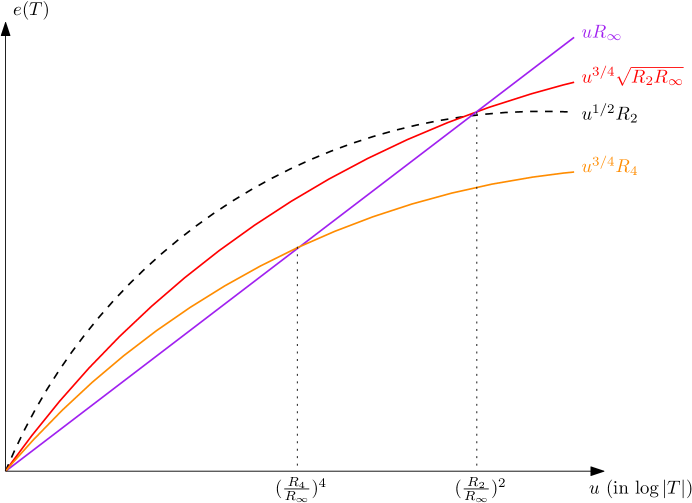
Figure 1: Phase transition in error bound

In this subsection we discuss the refinement on the proximity bound

$$e(T):=|r(T)-g(T)|,$$

where $r(T)$ and $g(T)$ are Rademacher and Gaussian complexities of T, respectively.

Let us define the following curves (associated with $T$):

(4.1) $$k(u)=u^{1/2}R_{2},\quad{\color[rgb]{1,0,0}t(u)=u^{3/4}\sqrt{R_{2}R_{\infty}}},\quad{\color[rgb]{1,.5,0}s_{1}(u)=u^{3/4}R_{4}},\quad{\color[rgb]{.75,0,.25}s_{2}(u)=uR_{\infty}}.$$

We shall introduce the following threshold values:

(4.2) $$u_{1}\equiv u_{1}(T):=(R_{4}/R_{\infty})^{4},\quad u_{2}:=(R_{2}/R_{\infty})^{2}.$$

Note that for any bounded set $T\subset\mathbb{R}^{n}$ we have $u_{1}(T)\leq u_{2}(T)\leq n$.

Recall that due to the fact that both processes $\{\langle\mathcal{E},t\rangle\}_{t\in T}$ and $\{\langle G,t\rangle\}_{t\in T}$ are sub-gaussian with constants approximately equal to $R_{2}(T)$ we readily get the (trivial) bound ^1.3 :

(4.3) $$|r(T)-g(T)|\leq CR_{2}\sqrt{\log|T|}.$$

Therefore, the error bound $t(u)$, ($u=\log|T|$) offered by Theorem 3.8 improves upon the trivial one when $u\ll u_{2}$. In view of $R_{4}\leq\sqrt{R_{2}R_{\infty}}$, one may check that in this range we have $s(u):=\max\{s_{1}(u),s_{2}(u)\}\leq t(u)$. More precisely, if $R_{4}=\delta\sqrt{R_{2}R_{\infty}}$, with $\delta\ll 1$ the window $[u_{1},u_{2}]=[\delta^{4}u_{2},u_{2}]$ of phase transition starts appearing where

$$s(u)=\begin{cases}s_{1}(u),&u\leq u_{1}\\ s_{2}(u),&u_{1}<u\leq u_{2}.\end{cases}$$

This refined error bound is illustrated in the Figure 1 above. Note that this is a dynamic phenomenon which depends on the index set $T$ and fades down as $u_{1}(T)\to u_{2}(T)$. However, the relative position of the aforementioned curves/parameters persists for each $T$.

Remark 4.1.

As in Theorem 1.1 we always have (due to sub-gaussian behavior [Ver18, Chapter 7]) that $\left\lvert g(T)\right\rvert$, $\left\lvert\mathbb{E}\sup_{t\in T}\langle\xi,t\rangle\right\rvert$ $\leq$ $CMR_{2}\sqrt{\log|T|}$ , and hence Theorem 3.8 is of interest only when its right-hand side is smaller than this quantity, that is, when

$$R_{4}\big{(}\log|T|\big{)}^{1/4}\,,\,R_{\infty}\big{(}\log|T|\big{)}^{1/2}\leq R_{2}.$$

Remark 4.2.

Notice that one cannot hope to generalize Talagrand’s Theorem 1.1 to include $\xi_{i}$ with sub-exponential tails. To see this, choose $T=\big{\{}e_{i}\mid 1\leq i\leq n\big{\}}$, that is, the canonical basis in $\mathbb{R}^{n}$, and $\xi_{i}$ to be $i.i.d.$ Laplace (two-sided exponential) distribution, that is, each $\xi_{i}$ has the density $\frac{1}{2}e^{-\left\lvert x\right\rvert}$ where $x\in\mathbb{R}$  . Then, the left-hand side of Theorem 1.1 is of the order $\log n$ whereas the right-hand side is of the order ${(\log n)}^{3/4}$.

4.1.1 Examples

In this subsection we construct a family of finite sets $T\subset\mathbb{R}^{n}$ for a wide spectrum of cardinalities with the additionally property $(R_{4}/R_{\infty})^{4}\ll(R_{2}/R_{\infty})^{2}$.

Consider any $A\subset\{-1,1\}^{n}$ such that $|A|=2^{k}$, where $k\ll n$. For a decreasing sequence of positive numbers $d_{1}>d_{2}>\ldots>d_{n}>0$ we consider the diagonal matrix

$$D:={\rm diag}(d_{1},\ldots,d_{n})=\begin{pmatrix}d_{1}&&&\\ &d_{2}&&\\ &&\ddots&\\ &&&d_{n}\end{pmatrix}.$$

Write $d$ for the vector $(d_{1},\ldots,d_{n})$ and set $T_{d}:=D(A)$, and notice that, for every $t\in T_{d}$, $t_{i}=\pm d_{i}$, and so $\left\lvert t_{i}\right\rvert=d_{i}$. Therefore, we get $\|t\|_{p}=\|d\|_{p}$ for all $p>0$, and thus

(4.4) $$u_{1}(T_{d})=(R_{4}/R_{\infty})^{4}=(\|d\|_{4}/\|d\|_{\infty})^{4},$$

(4.5) $$u_{2}(T_{d})=(R_{2}/R_{\infty})^{2}=(\|d\|_{2}/\|d\|_{\infty})^{2},$$

and $\log|T_{d}|\asymp k$. Taking into account the above features, we may construct subsets $T_{d}\subset\mathbb{R}^{n}$ with the property that $\log|T_{d}|<(R_{2}/R_{\infty})^{2}$ and $(R_{4}/R_{\infty})^{4}\ll(R_{2}/R_{\infty})^{2}$. For example, fix $k<\sqrt{n}$ and take $d_{j}\sim j^{-1/4}$ for $j\leq n$.

4.2 Further remarks

4.2.1 Universality

Talagrand in [Tal02] proved that the energy of the ground state of the Sherrington-Kirkpatrick’s (SK) model does not change when the Gaussian interactions $g_{ij}$ are replaced by Rademacher (symmetric Bernoulli) $\eta_{ij}$ interactions. In particular, he proved the following:

Corollary 4.3 (Talagrand).

Consider i.i.d. standard Gaussian random variables $(g_{ij})_{1\leq i<j\leq N}$ and i.i.d. Rademacher random variables $(\eta_{ij})_{1\leq i<j\leq N}$. Then

$$\left\lvert\frac{1}{N^{3/2}}\mathbb{E}\,\sup\sum_{1\leq i<j\leq N}g_{ij}\sigma_{i}\sigma_{j}-\frac{1}{N^{3/2}}\mathbb{E}\,\sup\sum_{1\leq i<j\leq N}\eta_{ij}\sigma_{i}\sigma_{j}\right\rvert\leq CN^{-1/4},$$

where the supremum is over $\sigma=(\sigma_{1},\sigma_{2},....,\sigma_{N})\in\{-1,1\}^{N}$.

Here, each $\sigma$ is interpreted as a configuration of an $N$-spin physical system. Above Corollary 4.3 was later generalized by Carmona and Hu in [CH06] to other interactions (environments) beyond Rademacher interactions $\eta_{ij}$.

Corollary 4.4 (Carmona and Hu).

Let $(g_{ij})_{1\leq i<j\leq N}$ be i.i.d. standard Gaussian random variables, and let $(\eta_{ij})_{1\leq i<j\leq N}$ be independent with $\mathbb{E}\eta_{ij}=0$ and $\mathbb{E}\eta_{ij}^{2}=1$. We have the following assertions:

1. If $\mu_{3}^{3}:=\max_{1\leq i<j\leq N}\mathbb{E}\left\lvert\eta_{ij}\right\rvert^{3}<\infty$, then

   (4.6) $$\left\lvert\frac{1}{N^{3/2}}\mathbb{E}\,\sup\sum_{1\leq i<j\leq N}g_{ij}\sigma_{i}\sigma_{j}-\frac{1}{N^{3/2}}\mathbb{E}\,\sup\sum_{1\leq i<j\leq N}\eta_{ij}\sigma_{i}\sigma_{j}\right\rvert\leq C\mu_{3}N^{-1/6}$$

2. Moreover, if $\mathbb{E}\eta_{ij}^{3}=0$ and $\mu_{4}^{4}:=\max_{1\leq i<j\leq N}\mathbb{E}\left\lvert\eta_{ij}^{4}\right\rvert<\infty$, then

   (4.7) $$\left\lvert\frac{1}{N^{3/2}}\mathbb{E}\,\sup\sum_{1\leq i<j\leq N}g_{ij}\sigma_{i}\sigma_{j}-\frac{1}{N^{3/2}}\mathbb{E}\,\sup\sum_{1\leq i<j\leq N}\eta_{ij}\sigma_{i}\sigma_{j}\right\rvert\leq C\mu_{4}N^{-1/4}$$

where $C>0$ is a universal constant.

We next show that the above results are special cases of a more general universality principle for the following random order-m tensors:

Corollary 4.5.

Let $\sigma=(\sigma_{1},\sigma_{2},\dots,\sigma_{N})\in\{-1,1\}^{N}\subset\mathbb{R}^{N}$ and define a random order-m tensor as follows:

$$(i_{1},i_{2},\dots,i_{m})\mapsto\eta_{i_{1}i_{2}....i_{m}}\prod_{j=1}^{m}\sigma_{i_{j}}$$

where $1\leq i_{1}<i_{2}<\dots<i_{m}\leq N$, and $1<m<(N-1)$. Let $g_{i_{1}i_{2}....i_{m}}$ be $i.i.d.$ standard Gaussian random variables, and let $\eta_{i_{1}i_{2}....i_{m}}$ be independent with $\mathbb{E}\,\eta_{i_{1}i_{2}....i_{m}}=0$ and $\mathbb{E}\,{\eta_{i_{1}i_{2}....i_{m}}^{2}}=1$.

1. If $\mu_{3}^{3}:=\max_{1\leq i_{1}<i_{2}<\dots<i_{m}\leq N}\mathbb{E}\left\lvert\eta_{i_{1}i_{2}....i_{m}}\right\rvert^{3}<\infty$, then

   $$\left\lvert\frac{1}{{\binom{N}{m}}^{1/2}N^{1/2}}\mathbb{E}\sup_{\sigma}\sum_{1\leq i_{1}<i_{2}<\dots<i_{m}\leq N}\eta_{i_{1}i_{2}....i_{m}}\prod_{j=1}^{m}\sigma_{i_{j}}-\frac{1}{{\binom{N}{m}}^{1/2}N^{1/2}}\mathbb{E}\sup_{\sigma}\sum_{1\leq i_{1}<i_{2}<\dots<i_{m}\leq N}g_{i_{1}i_{2}....i_{m}}\prod_{j=1}^{m}\sigma_{i_{j}}\right\rvert\leq C\mu_{3}\Bigg{(}{\frac{N}{\binom{N}{m}}}\Bigg{)}^{1/6}.$$

2. Moreover, if $\mathbb{E}\eta_{i_{1}i_{2}....i_{m}}^{3}=0$, and $\mu_{4}^{4}:=\max_{1\leq i_{1}<i_{2}<\dots<i_{m}\leq N}\mathbb{E}\left\lvert\eta_{i_{1}i_{2}....i_{m}}\right\rvert^{4}<\infty$, then

   $$\left\lvert\frac{1}{{\binom{N}{m}}^{1/2}N^{1/2}}\mathbb{E}\sup_{\sigma}\sum_{1\leq i_{1}<i_{2}<\dots<i_{m}\leq N}\eta_{i_{1}i_{2}....i_{m}}\prod_{j=1}^{m}\sigma_{i_{j}}-\frac{1}{{\binom{N}{m}}^{1/2}N^{1/2}}\mathbb{E}\sup_{\sigma}\sum_{1\leq i_{1}<i_{2}<\dots<i_{m}\leq N}g_{i_{1}i_{2}....i_{m}}\prod_{j=1}^{m}\sigma_{i_{j}}\right\rvert\leq C\mu_{4}\Bigg{(}{\frac{N}{\binom{N}{m}}}\Bigg{)}^{1/4},$$

where $C>0$ is a universal constant.

Proof. Use Corollary 3.4 with $T=\Bigg{\{}\bigg{(}\frac{\prod_{j=1}^{m}\sigma_{i_{j}}}{{\binom{N}{m}}^{1/2}N^{1/2}}\bigg{)}_{1\leq i_{1}<i_{2}<\dots<i_{m}\leq N}\,\,\,\Big{|}\,\,\,\sigma=(\sigma_{1},....,\sigma_{N})\in\{-1,1\}^{N}\Bigg{\}}$.

We refer the reader to [Tal03, Chapter 2] for an interpretation of the above result in the context of Spin glasses.

4.2.2 A more general setting

Let us note that the results in Section 3 can be formulated for an arbitrary measure $\mu$ supported on the index set $T$. To see this note that for a finite set $T$ we may write

$$F_{\beta}(x)=\frac{1}{\beta}\log\left(\sum_{t\in T}e^{\beta\langle x,t\rangle}\right)=\frac{\log|T|}{\beta}+\frac{1}{\beta}\log\left(\int_{T}e^{\beta{\langle x,t\rangle}}\,d\nu(t)\right),$$

where $\nu$ is the uniform probability measure on $T$. The latter integral is an appropriate re-scaling of the logarithmic Laplace transform of $\nu$. Recall that for a probability measure $\mu$ on $\mathbb{R}^{n}$ the logarithmic Laplace transform of $\mu$ is defined by

(4.8) $$\Lambda_{\mu}(\xi)\stackrel{{\scriptstyle\rm def}}{{=}}\log\left(\int_{\mathbb{R}^{n}}e^{\langle\xi,x\rangle}\,d\mu(x)\right),\quad\xi\in\mathbb{R}^{n}.$$

We refer the reader to [LaW08] and the references therein for background information on the log-Laplace transform. With this notation the corresponding Gibbs’ measure is given by

(4.9) $$\frac{d\mu_{\xi}}{d\mu}(t)=\frac{e^{\langle\xi,t\rangle}}{\int e^{\langle\xi,t\rangle}\,d\mu(t)}.$$

Thus, differentiation under the integral sign yields

(4.10) $$\nabla\Lambda_{\mu}(\xi)=(\mathbb{E}_{\mu_{\xi}}[\ell_{i}])_{i=1}^{n},\quad{\rm Hess}\,\Lambda_{\mu}(\xi)={\rm Cov}(\mu_{\xi}).$$

See e.g., [Kla06, KM12] for details. Furthermore, Lemma 2.2 becomes as follows:

Lemma 4.6.

Let $\mu$ be a probability measure supported on the bounded $T\subset\mathbb{R}^{n}$. Then,

(4.11) $$\left|\frac{\partial^{3}}{\partial\xi_{i}^{3}}\Lambda_{\mu}(\xi)\right|\leq 6\mathbb{E}_{\mu_{\xi}}\left[|\ell_{i}|^{3}\right]\leq 6\max_{t\in T}|t_{i}|^{3},\quad\left|\frac{\partial^{4}}{\partial\xi_{i}^{4}}\Lambda_{\mu}(\xi)\right|\leq 26\mathbb{E}_{\mu_{\xi}}\left[|\ell_{i}|^{4}\right]\leq 26\max_{t\in T}|t_{i}|^{4}.$$

Using the above Lemma, one can prove the following extension of Proposition 3.3:

Proposition 4.7.

Let $T\subset\mathbb{R}^{n}$ be a bounded set and let be $\mu$ be a probability measure on $T$. Let $\xi=(\xi_{1},\ldots,\xi_{n})$ be a random vector with independent coordinates such that $\mathbb{E}\xi_{i}=0$ and $\mathbb{E}\xi_{i}^{2}=1$. We have the following cases:

1. If $\sigma_{3}^{3}:=\max_{i\leq n}\mathbb{E}|\xi_{i}|^{3}<\infty$, then we have

   (4.12) $$\left|\mathbb{E}\Lambda_{\mu}(\xi)-\mathbb{E}\Lambda_{\mu}(G)\right|\leq C\sigma_{3}^{3}\|(e_{1},\ldots,e_{n})\|_{\ell_{3}(T)}^{3}.$$

2. Furthermore, if $\mathbb{E}\xi_{i}^{3}=0$ for all $i\leq n$ and $\sigma_{4}^{4}:=\max_{i\leq n}\mathbb{E}\xi_{i}^{4}<\infty$, then we have

   (4.13) $$\left|\mathbb{E}\Lambda_{\mu}(\xi)-\mathbb{E}\Lambda_{\mu}(G)\right|\leq C\sigma_{4}^{4}\|(e_{1},\ldots,e_{n})\|_{\ell_{4}(T)}^{4},$$

   where $C>0$ is a universal constant.
   

One may generalize Lemma 3.5 to the following:

Lemma 4.8.

Let $T\subset\mathbb{R}^{n}$ be bounded and let $\mu$ be a probability measure supported on $T$. For any $f:T\to[0,\infty)$ we may define $\psi(x)=\log\mathbb{E}_{\mu_{x}}[f]$. Then, for all $x,y\in\mathbb{R}^{n}$, we have

$$|\psi(x)-\psi(y)|\leq\sup_{t\in T}|\langle t,x-y\rangle|.$$

In particular, $|\psi(x)-\psi(y)|\leq R_{\infty}(T)\|x-y\|_{1}$ for all $x,y\in\mathbb{R}^{n}$.

Using the above lemma along with Lemma 4.6, one may obtain the following extension of Proposition 3.6 :

Proposition 4.9.

Let $T\subset\mathbb{R}^{n}$ be bounded and let $\mu$ be a probability measure supported on $T$. Then, for any random vector $\xi=(\xi_{1},\ldots,\xi_{n})$ with independent coordinates, where $\mathbb{E}\xi_{i}=\mathbb{E}\xi_{i}^{3}=0$, $\mathbb{E}\xi_{i}^{2}=1$ and $|\xi_{i}|\leq M$ a.s. for all $i\leq n$, we have that

(4.14) $$\left|\mathbb{E}\Lambda_{\mu}(\xi)-\mathbb{E}\Lambda_{\mu}(G)\right|\leq CM^{4}R_{4}^{4}(T)e^{MR_{\infty}(T)},$$

where $C>0$ is a universal constant.

References

- [AAGM15] Shiri Artstein-Avidan, Apostolos Giannopoulos, and Vitali D. Milman. Asymptotic geometric analysis. Part I, volume 202 of Mathematical Surveys and Monographs. American Mathematical Society, Providence, RI, 2015.
- [ALMT14] Dennis Amelunxen, Martin Lotz, Michael B McCoy, and Joel A Tropp. Living on the edge: Phase transitions in convex programs with random data. Information and Inference: A Journal of the IMA, 3(3):224–294, 2014.
- [Bar16] Alexander Barvinok. Combinatorics and complexity of partition functions, volume 30 of Algorithms and Combinatorics. Springer, Cham, 2016.
- [BGL14] Dominique Bakry, Ivan Gentil, and Michel Ledoux. Analysis and geometry of Markov diffusion operators, volume 348 of Grundlehren der mathematischen Wissenschaften [Fundamental Principles of Mathematical Sciences]. Springer, Cham, 2014.
- [BL14] Witold Bednorz and Rafal Latala. On the boundedness of Bernoulli processes. Ann. of Math. (2), 180(3):1167–1203, 2014.
- [BM02] Peter L Bartlett and Shahar Mendelson. Rademacher and gaussian complexities: Risk bounds and structural results. Journal of Machine Learning Research, 3(Nov):463–482, 2002.
- [CGS11] Louis H. Y. Chen, Larry Goldstein, and Qi-Man Shao. Normal approximation by Stein’s method. Probability and its Applications (New York). Springer, Heidelberg, 2011.
- [CH06] Philippe Carmona and Yueyun Hu. Universality in sherrington–kirkpatrick’s spin glass model. In Annales de l’Institut Henri Poincare (B) Probability and Statistics, volume 42, pages 215–222. Elsevier, 2006.
- [Cha05] Sourav Chatterjee. An error bound in the sudakov-fernique inequality. arXiv preprint math/0510424, 2005.
- [Cha14] Sourav Chatterjee. A short survey of Stein’s method. In Proceedings of the International Congress of Mathematicians—Seoul 2014. Vol. IV, pages 1–24. Kyung Moon Sa, Seoul, 2014.
- [Kla06] B. Klartag. On convex perturbations with a bounded isotropic constant. Geom. Funct. Anal., 16(6):1274–1290, 2006.
- [KM11] Satish Babu Korada and Andrea Montanari. Applications of the lindeberg principle in communications and statistical learning. IEEE transactions on information theory, 57(4):2440–2450, 2011.
- [KM12] Bo’az Klartag and Emanuel Milman. Centroid bodies and the logarithmic Laplace transform—a unified approach. J. Funct. Anal., 262(1):10–34, 2012.
- [LaW08] R. Latał a and J. O. Wojtaszczyk. On the infimum convolution inequality. Studia Math., 189(2):147–187, 2008.
- [OT18] Samet Oymak and Joel A Tropp. Universality laws for randomized dimension reduction, with applications. Information and Inference: A Journal of the IMA, 7(3):337–446, 2018.
- [RV08] Mark Rudelson and Roman Vershynin. On sparse reconstruction from Fourier and Gaussian measurements. Comm. Pure Appl. Math., 61(8):1025–1045, 2008.
- [Ste72] Charles Stein. A bound for the error in the normal approximation to the distribution of a sum of dependent random variables. In Proceedings of the Sixth Berkeley Symposium on Mathematical Statistics and Probability (Univ. California, Berkeley, Calif., 1970/1971), Vol. II: Probability theory, pages 583–602. Univ. California Press, Berkeley, CA, 1972.
- [Tal87] Michel Talagrand. Regularity of Gaussian processes. Acta Math., 159(1-2):99–149, 1987.
- [Tal96] Michel Talagrand. Majorizing measures: the generic chaining. The Annals of Probability, 24(3):1049–1103, 1996.
- [Tal01] Michel Talagrand. Majorizing measures without measures. Annals of probability, pages 411–417, 2001.
- [Tal02] Michel Talagrand. Gaussian averages, Bernoulli averages, and Gibbs’ measures. Random Structures & Algorithms, 21(3-4):197–204, 2002.
- [Tal03] Michel Talagrand. Spin glasses: a challenge for mathematicians, volume 46 of Ergebnisse der Mathematik und ihrer Grenzgebiete. 3. Folge. A Series of Modern Surveys in Mathematics. Cavity and mean field models. [Results in Mathematics and Related Areas. 3rd Series. A Series of Modern Surveys in Mathematics]. Springer-Verlag, Berlin, 2003.
- [Tal21] Michel Talagrand. Upper and lower bounds for stochastic processes—decomposition theorems, volume 60 of Ergebnisse der Mathematik und ihrer Grenzgebiete. 3. Folge. A Series of Modern Surveys in Mathematics [Results in Mathematics and Related Areas. 3rd Series. A Series of Modern Surveys in Mathematics]. Springer, Cham, second edition, ©2021.
- [TH15] Christos Thrampoulidis and Babak Hassibi. Isotropically random orthogonal matrices: Performance of lasso and minimum conic singular values. In 2015 IEEE International Symposium on Information Theory (ISIT), pages 556–560, 2015.
- [Ver18] Roman Vershynin. High-dimensional probability: An introduction with applications in data science, volume 47. Cambridge university press, 2018.