Equilibrium parametric amplification in Raman-cavity hybrids

Abstract

Parametric resonances and amplification have led to extraordinary photo-induced phenomena in pump-probe experiments. While these phenomena manifest themselves in out-of-equilibrium settings, here, we present the striking result of parametric amplification in equilibrium. In particular, we demonstrate that quantum and thermal fluctuations of a Raman-active mode amplifies light inside a cavity, at equilibrium, when the Raman mode frequency is twice the cavity mode frequency. This noise-driven amplification leads to the creation of an unusual parametric Raman polariton, intertwining the Raman mode with cavity squeezing fluctuations, with smoking gun signatures in Raman spectroscopy. In the resonant regime, we show the emergence of not only quantum light amplification but also localization and static shift of the Raman mode. Apart from the fundamental interest of equilibrium parametric amplification our study suggests a resonant mechanism for controlling Raman modes and thus matter properties by cavity fluctuations. We conclude by outlining how to compute the Raman-cavity coupling, and suggest possible experimental realizations.

Introduction.- Driving condensed matter with light provides a methodology of controlling its properties in an active, dynamic fashion, in contrast to the established, static methods, as reflected in recent scientific studies A. de la Torre, D. M. Kennes, M. Claassen, S. Gerber, J. W. McIver, and M. A. Sentef (2021); Basov et al. (2017); Bloch et al. (2022); Kennes and Rubio (2023). In this effort, driving matter with laser light has proved to be a remarkably versatile tool in engineering properties of quantum materials such as controlling ferro-electricity Nova et al. (2019), magnetism Disa et al. (2023); Siegrist et al. (2019); Beaulieu et al. (2021); Boström et al. (2020), superconductivity Mitrano et al. (2016); Budden et al. (2021); Rowe et al. (2023); Chattopadhyay et al. (2023); von Hoegen et al. (2022); Michael et al. (2020), topological features McIver et al. (2020) and charge ordering Kogar et al. (2020); Dolgirev et al. (2023). Even more interestingly, driving with light has provided the possibility to create novel non-equilibrium states. A notable example includes photonic time crystals Lyubarov et al. (2022); Michael et al. (2022, 2023); Haque et al. (2023); Dolgirev et al. (2022), materials exhibiting periodic variation in properties over time that can function as parametric amplifiers for light. Another example is time crystals, denoting a robust, collective dynamical many-body state, in which the response of observables oscillates subharmonically Else et al. (2020); Zhang et al. (2017); Choi et al. (2017); Keßler et al. (2021); Kongkhambut et al. (2021); Taheri et al. (2022); Zaletel et al. (2023); Ojeda Collado et al. (2021); Collado et al. (2023).

The conceptual approach of dynamical control with light can be extended to the equilibrium domain through cavity-matter hybrids, see e.g. Schlawin et al. (2022); Curtis et al. (2023); Ruggenthaler et al. (2018). This advancement of control via light involves replacing laser driving by quantum light fluctuations which are strongly coupled to matter through resonant photonic structures, such as cavities Jarc et al. (2022), plasmonic resonators Appugliese et al. (2022), surfaces hosting surface phonon polaritons Lenk et al. (2022); Eckhardt et al. (2023) and photonic crystals Baydin et al. (2023). The feasibility of this approach has been demonstrated experimentally, with examples including manipulation of transport Orgiu et al. (2015), control of superconducting properties A. Thomas, E. Devaux, K. Nagarajan, T. Chervy, M. Seidel, D. Hagenmüller, S. Schütz, J. Schachenmayer, C. Genet, G. Pupillo, and T. W. Ebbesen (2019), magnetism A. Thomas, E. Devaux, K. Nagarajan, G. Rogez, M. Seidel, F. Richard, C. Genet, M. Drillon, and T. W. Ebbesen (2021), topological features Appugliese et al. (2022) and cavity control of chemical reactivity Thomas et al. (2019); Nagarajan et al. (2021); Schäfer et al. (2022).

In this paper, we demonstrate that quantum and thermal noise of a Raman-active mode, can amplify cavity fluctuations in equilibrium. We emphasize that parametric amplification generally occurs in driven systems while here we present it in the context of an equilibrium amplification process. This amplification can in turn be used to resonantly control properties of matter and constitutes a novel method of light control, for Raman-cavity systems.

Our starting point is the nonlinear coupling between Raman active collective modes and light. Here Raman-active modes could be Raman phonons Först et al. (2011), molecular vibrations Chattopadhyay et al. (2023), Higgs modes in superconductors R. Matsunaga, N. Tsuji, H. Fujita, A. Sugioka, K. Makise, Y. Uzawa, H. Terai, Z. Wang, H. Aoki and R. Shimano (2014); Buzzi et al. (2021); Collado et al. (2018) and amplitude modes in charge density waves Dolgirev et al. (2023) that are even under inversion symmetry, and the electric field of a local cavity mode Juraschek et al. (2021). Therefore, at leading order, the Raman-light Hamiltonian reads $H_{Raman-light}=\lambda QE_{cav}^{2}$ where $E_{cav}$ is the electric field in the cavity, $Q$ is the coordinate of the Raman collective mode and $\lambda$ is the light-matter coupling. This quadratic coupling includes parametrically resonant processes of the type $\hat{a}^{\dagger}\hat{a}^{\dagger}\hat{b}+\hat{a}\hat{a}\hat{b}^{\dagger}$ where $\hat{a}$ and $\hat{b}$ are the photon and Raman annihilation operators respectively. In the presence of coherent Raman oscillations, $\langle b(t)\rangle=A_{0}e^{i\omega_{R}t}$, at the Raman frequency $\omega_{R}$, the above coupling leads to exponential growth of the light field when the cavity frequency $\omega_{c}$ satisfies the parametric resonant condition, $2\omega_{c}=\omega_{R}$. This observation naturally leads to the question: can a randomly fluctuating field coming from Raman quantum fluctuations also amplify light? We find that the answer is yes which we demonstrate below.

To study this phenomenon, we use an open Truncated-Wigner approximation method (open TWA) Polkovnikov (2010); Cosme et al. (2019); Skulte et al. (2023) to simulate the semi-classical dynamics of the Raman-cavity hybrids in the quantum fluctuation regime. We also determine the signatures of equilibrium parametric amplification in Raman spectroscopy (Fig. 1 (a)). We find that a prominent feature of parametric resonance and equilibrium light amplification is the appearance of two Raman polariton branches in Raman spectroscopy as shown in Fig. 1(b). We call this polariton parametric Raman polariton and its formation is attributed to the nonlinear process of mixing squeezed photon fluctuations with the Raman coordinate. This is substantially different to the existent polariton panorama where polaritons typically arise from a linear coupling between matter degrees of freedom and light Basov et al. (2021). To quantify the coupling between the Raman mode and the cavity, we compute the resonance splitting between the upper and lower parametric Raman polariton. This is a nonlinear extension of the usual Rabi-splitting in the case of infrared active phonon polaritons Jarc et al. (2022). We use a frequency dependent Gaussian theory to provide an analytical expression for this splitting as a function of the coupling strength which agrees well with the simulations.

The key features of the parametric Raman polariton are as follows: (i) The vacuum fluctuations of the cavity mode are amplified. (ii) The fluctuations of the Raman are reduced, in response to the amplification of the cavity fluctuations. This corresponds to a localization of the Raman mode. (iii) The average position of the Raman mode is statically shifted due to the cavity fluctuations as shown schematically in Fig. 1(c). These observations suggest that this mechanism can be used to resonantly modify and control both the Raman mode and the cavity in equilibrium. Furthemore we conclude by proposing realistic experimental set-ups where this phenomenon can be observed.

Raman-Cavity Model $\&$ Raman spectroscopy.- We consider a model, in which cavity field fluctuations are locally coupled to a Raman coordinate. The Hamiltonian for this system is given by:

$$\frac{H}{\hbar}=\omega_{c}\hat{a}^{\dagger}\hat{a}+\omega_{R}\hat{b}^{\dagger}\hat{b}+g\left(\hat{b}^{\dagger}+\hat{b}\right)\left(\hat{a}^{\dagger}+\hat{a}\right)^{2}+\frac{g_{4}}{4}\left(\hat{a}^{\dagger}+\hat{a}\right)^{4}.$$ (1)

The cavity creation (annihilation) operator is $\hat{a}^{\dagger}$ ($\hat{a}$) and $\omega_{c}$ is the cavity frequency. $\hat{b}^{\dagger}$ and $\hat{b}$ are the creation and annihilation operators for the Raman mode of frequency $\omega_{R}$ and $g$ is the coupling strength between the cavity and Raman mode. To connect these operators to the electric field in the cavity we require that $\hat{E}_{cav}^{2}=E^{2}_{0}\left(\hat{a}+\hat{a}^{\dagger}\right)^{2}$, where $E^{2}_{0}$ is the nonzero quantum noise of the electric field in the cavity that can be measured experimentally Appugliese et al. (2022), while the cavity itself is in equilibrium, $\left<\hat{E}_{cav}\right>=0$ and the Raman coordinate is given by $\hat{Q}=\frac{\hat{b}^{\dagger}+\hat{b}}{\sqrt{2\omega_{R}}}$. The last term of strength $g_{4}$ is an $\hat{E}_{cav}^{4}$ type of nonlinearity necessary to make the system stable for finite coupling $g<\sqrt{g_{4}\omega_{R}}/2$, a condition that is found analytically in the Supplementary Information (SI).

We propose Raman spectroscopy as a natural probe for Raman polaritons (see Fig. 1 (a)). The spectroscopic protocol consists of an incoming probe laser of frequency $\omega_{p}$ that can be scattered to free space as outgoing photons with frequency $\omega_{s}$ after interacting with the Raman medium through a Stimulated Raman Scattering (SRS) (shown scematically in Fig. 1 (a)).

The probe is assumed to be a coherent light-source with an associated electric field $E_{p}(t)=E^{0}_{p}sin(\omega_{p}t)$ whereas the scattered photons are described by the Hamiltonian $H_{s}/\hbar=\omega_{s}\hat{a}_{s}^{\dagger}\hat{a}_{s}$. The SRS Hamiltonian can be written as:

$$\frac{H_{p}}{\hbar}=g_{s}E_{p}(t)\left(\hat{b}^{\dagger}+\hat{b}\right)\left(\hat{a}_{s}^{\dagger}+\hat{a}_{s}\right)$$ (2)

where $\hat{a}_{s}^{\dagger}$ ($\hat{a}_{s}$) is the creation (annihilation) operator for scattered photons and $g_{s}$ the coupling between the Raman mode and photons being scattered. The requirement for weak probing is that $g_{s}E^{0}_{p}$ is much smaller than the magnitude of the energies of the system such as $g$, as we will choose in the following.

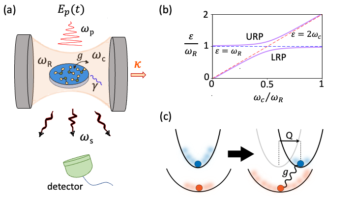
Figure 1: Parametric Raman Polaritons. (a) Sketch of a Raman medium (blue) coupled to a single-photon cavity mode of frequency $\omega_{c}$ (light-red shading) with a constant coupling $g$. Light can leak out of the cavity at a total decay rate $\kappa$ while $\gamma$ represents the damping associated to the Raman mode $\omega_{R}$. The wavy lines at the top and bottom represent a Raman spectroscopy scheme in which a probe field $E_{p}(t)$ of frequency $\omega_{p}$ is sent into the sample, and a detector (in green) collects the scattered photons at different frequencies $\omega_{s}$ giving information about the hybrid Raman-cavity system. (b) Representative Raman spectrum (in purple) in which an avoided crossing appears at the resonant condition $\omega_{R}=2\omega_{c}$ indicating the existence of two branches, the upper (URP) and lower (LRP) Raman polaritons. (c) Sketch of how Raman (blue) and cavity (red) properties are modified due to the coupling $g$. Full circles represent the equilibrium position and shaded regions indicate fluctuations. In the resonant regime the cavity fluctuations are amplified while the Raman mode is statically shifted and localized, i.e. its fluctuations decrease.

Considering the total Hamiltonian $H_{t}=H+H_{p}+H_{s}$ we derive the corresponding Heisenberg-Langevin equations of motion and use the open TWA method to solve the dynamics. This semi-classical phase-space method captures the lowest order quantum effects beyond mean-field treatment as extensively demonstrated in different contexts Polkovnikov (2010); Cosme et al. (2019); Kongkhambut et al. (2022); Skulte et al. (2023) and consists of sampling the initial states from the corresponding Wigner distribution to take into account the quantum uncertainty. The semiclassical equations of motion for the complex fields $a$, $b$ and $a_{s}$ associated with cavity photons, Raman motion and scattered photons operators are given by

$$\begin{split}i\partial_{t}{a}=&\omega_{c}a+2g(a+a^{*})(b+b^{*})+g_{4}(a+a^{*})^{3}\\ &-i\kappa a+i\xi_{a},\end{split}$$ (3)

$$\begin{split}i\partial_{t}{b}=&\omega_{R}b+g(a+a^{*})^{2}+g_{s}E_{p}(t)(a_{s}+a_{s}^{*})\\ &-i\gamma(b-b^{*})/2-\xi_{b},\end{split}$$ (4)

$$i\partial_{t}{a_{s}}= \omega_{s}a_{s}+g_{s}E_{p}(t)(b+b^{*})-i\kappa_{s}a_{s}+i\xi_{s},$$ (5)

Here $\kappa$, $\gamma$ and $\kappa_{s}$ are the decay rates associated with the cavity, Raman and scattered photon field while $\xi_{a}$, $\xi_{b}$ and $\xi_{s}$ are sources of Gaussian noise obeying the autocorrelation relations $\left<\xi_{a}^{*}(t_{1})\xi_{a}(t_{2})\right>=\kappa\delta(t_{1}-t_{2})$, $\left<\xi_{b}(t_{1})\xi_{b}(t_{2})\right>=\gamma\delta(t_{1}-t_{2})$ and $\left<\xi_{s}^{*}(t_{1})\xi_{s}(t_{2})\right>=\kappa_{s}\delta(t_{1}-t_{2})$. $\xi_{a}$ and $\xi_{s}$ are complex-valued whereas $\xi_{b}$ is real-valued and, along with the damping term, enters only in the equation of motion for the imaginary part of the Raman field which is associated with the momentum of the Raman mode. The choice for the Raman mode is motivated by the Brownian motion in which the frictional force is proportional to the velocity.

We simulate the quantum Langevin Eqs. (3-5) using a stochastic ordinary differential equation (ODE) solver and compute relevant observables in the steady state. To initiate the dynamics we ramp out the coupling $g$ from zero to a finite value and wait for the steady state before turning on the probe field $E_{p}(t)$ (see SI for details). In particular, we define the Raman spectrum as the number of scattered photons $n_{s}=|a_{s}|^{2}$ as a function of their frequencies which is computed after a certain time of exposure to the probe field (see SI).

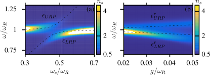
Figure 2: (a) Raman spectra $n_{s}\left(\omega\right)$ for different cavity frequencies $\omega_{c}$. We consider a probe laser of strength $g_{s}E_{p}^{0}=0.04\omega_{R}$ and frequency $\omega_{p}=5\omega_{R}$ with $g=0.04\omega_{R}$, $g_{4}=\kappa=\gamma=\kappa_{s}=0.01\omega_{R}$. (b) Raman polariton branches at resonance as a function of the coupling $g$ on resonance, $\overline{\omega}_{c}=\omega_{R}/2$. In both panels, the dashed black lines correspond to an analytical solution using a Gaussian approximation theory.

Parametric Raman polaritons.- In Fig. 2 (a) we show the Raman spectra $n_{s}(\omega)$ for different cavity frequencies and a fixed coupling strength where $\omega=\omega_{p}-\omega_{s}$ is the Raman shift. Away from resonance we see only one peak at $\omega\approx\omega_{R}$, which corresponds to the Stokes peak Cardona and G.Güntherodt (1982); Brüesch (1986) of the Raman mode . Near the resonance at $\omega_{c}=\omega_{R}/2$ a second peak appears showing an avoided crossing, which signals the existence of a Raman polariton. To gain insight into the two polariton branches found numerically using the TWA method, we employ a Gaussian approximation. Within this method, outlined in the SI, we find that the two polariton branches arise from resonant coupling between the Raman phonon mode oscillating at $\omega_{R}$ and Gaussian squeezing oscillations of the photon, oscillating at $2\omega_{c}$ leading to a new hybrid Raman polariton. We have computed analytically the dispersion of the lower and upper Raman polariton branches which are plotted with black dashed lines in Fig. 2(a), showing good agreement with the two numerical peaks in the Raman spectrum (indicated by $\epsilon_{LRP}$ and $\epsilon_{URP}$). The exact position of the avoided crossing is shifted to the left compared to the condition $\omega_{c}=\omega_{R}/2$, due to the renormalization of the cavity frequency by nonlinear interactions. Within the Gaussian approximation the effective cavity frequency is found to be $\bar{\omega}_{c}=\omega_{c}-12g^{2}/\omega_{R}+3g_{4}$ so the improved estimate of the resonance condition is $\bar{\omega}_{c}=\omega_{R}/2$.

To quantify the strength of the Raman-cavity coupling, we define the Raman Rabi splitting as the difference between the upper and lower Raman polaritons on resonance, $2\delta=\epsilon_{URP}(\bar{\omega}_{c}=\omega_{R}/2)-\epsilon_{LRP}(\bar{\omega}_{c}=\omega_{R}/2)$. In Fig. 2(b) we plot the dependence of the Raman polariton branches on resonance $\epsilon^{r}_{URP}=\epsilon_{URP}(\bar{\omega}_{c}=\omega_{R}/2)$ and $\epsilon^{r}_{LRP}=\epsilon_{LRP}(\bar{\omega}_{c}=\omega_{R}/2)$ on the coupling strength $g$, and overlay the analytical prediction in black dashed lines. The Rabi splitting grows linearly with the coupling strength $g$ and is given analytically by the expression:

$$\begin{split}\delta=\sqrt{2\langle\hat{x}^{2}\rangle\omega_{R}}\left(1-27g_{4}\langle\hat{x}^{2}\rangle^{3}/2\right)g+\mathcal{O}(g^{3}).\end{split}$$ (6)

Interestingly, the Gaussian theory suggests that the Rabi splitting could be parametrically enhanced by the cavity quantum fluctuations $\langle\hat{x}^{2}\rangle$, where $\hat{x}=\frac{a+a^{\dagger}}{\sqrt{2\omega_{c}}}$. Perturbatively, $\langle\hat{x}^{2}\rangle=\frac{1}{2\omega_{c}}+\mathcal{O}(g^{2})$, which is the value we use in Eq. (6) to plot the dashed lines in Fig.2(b).

Equilibrium parametric amplification- While Raman spectroscopy provides experimental evidence for strong Raman-cavity coupling, we now expand the discussion to the equilibrium properties of the Raman polariton system which exhibit equilibrium parametric amplification. This phenomenology corresponds to the amplification of photon fluctuations accompanied by a localization of Raman mode fluctuations, i.e. suppression of fluctuations, depicted schematically in Fig. 1 (c).

To illustrate the modification of each subsystem due to the Raman-cavity coupling, we determine the deviation of the Raman and cavity fluctuations $\delta Q^{2}$ and $\delta x^{2}$ from the uncoupled case given by

$$\delta Q^{2}=\frac{\left<\hat{Q}^{2}\right>-\left<\hat{Q}^{2}\right>_{0}}{\left<\hat{Q}^{2}\right>_{0}},\\ \delta x^{2}=\frac{\left<\hat{x}^{2}\right>-\left<\hat{x}^{2}\right>_{0}}{\left<\hat{x}^{2}\right>_{0}}$$ (7)

where $\left<...\right>$ denotes the expectation value for a finite coupling $g$ and $\left<...\right>_{0}$ the expectation value in the absence of coupling and cavity nonlinearities ($g=g_{4}=0$). As in the previous section, $\hat{x}=\frac{\hat{a}^{\dagger}+\hat{a}}{\sqrt{2\omega_{c}}}$, is the cavity coordinate which is related to the electric field, $\hat{E}_{cav}=\sqrt{2\omega_{c}}E_{0}\hat{x}$, where $E_{0}$ is the electric field amplitude of the noise of the cavity mode. Note that also $\delta x^{2}=\frac{\langle\hat{E}_{cav}^{2}\rangle-\langle\hat{E}_{cav}^{2}\rangle_{0}}{\langle\hat{E}_{cav}^{2}\rangle_{0}}$, and denotes the amplification of the quantum fluctuations in the electric field. To compute these Raman and cavity fluctuations we set the probe field $E_{p}(t)$ in Eqs. (3-5) to zero and average over steady states of the Langevin equations of motion (see SI for details).

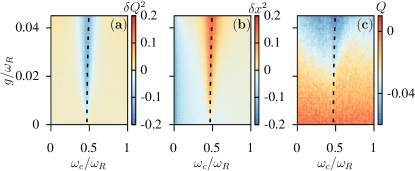
Figure 3: (a), (b) Variation of Raman and cavity fluctuations compared to the uncoupled case $g=0$ (see text) for different cavity frequencies and coupling strengths $g$. (c) Raman displacement. The dashed lines represent the parametric resonant condition $\omega_{R}=2\bar{\omega}_{c}$. On resonance, the main features of parametric Raman polaritons appear: localization (a) and shift (c) of the Raman mode in favor of cavity field amplification (b). The decay rates and nonlinear interaction $g_{4}$ are the same as in Fig. 2.

In Fig. 3 we show $\delta Q^{2}$ and $\delta x^{2}$ as well as the Raman coordinate $Q=\left<\hat{Q}\right>$ for different cavity frequencies and coupling strengths $g$. In all cases, a clear resonance can be seen around $\omega_{c}\approx\omega_{R}/2$ indicating a resonant regime in which both the Raman mode and cavity fluctuations are strongly modified. In this regime, the Raman fluctuations are suppressed by the cavity, $\delta Q^{2}<0$, so the Raman mode is localized while the cavity fluctuations are amplified by the Raman mode $\delta x^{2}>0$. Outside this resonant region the Raman fluctuations are unaffected and remain the same as in free space ($\delta Q^{2}\approx 0$). In a similar way, for off-resonant cavity frequencies, quantum vacuum fluctuations remain practically unchanged meaning that the Raman medium barely perturbs the photon field ($\delta x^{2}\approx 0$). This observation justifies our choice to consider the coupling of a single cavity mode with a single Raman mode: due to the resonant character of the interaction, we expect that other off-resonant modes do not contribute.

For the parameters used in Fig. 3, on resonance and close to the instability $g\approx\sqrt{g_{4}\omega_{R}}/2$, the Raman mode is strongly localized by $\sim 20\%$ compared to the case of Raman fluctuations in free space while the photon field increases by the same amount with respect to the empty cavity case, even though the coupling is only $g\sim 4\%\omega_{R}$. We would like to emphasize that the coupling values $g$ used in Fig. 2 and Fig. 3 are of the same order of magnitude as the decay rates $\gamma$ and $\kappa$. Therefore the system is between the weak and strong coupling regime but not in the ultrastrong coupling situation ($g>\omega_{c}$) where these resonant effects may be more pronounced Frisk Kockum et al. (2019).

In Fig. 3 (c) the expectation value of the Raman coordinate $Q$ is shown as a function of coupling strength $g$ and cavity frequency $\omega_{c}$. A clear shift of the Raman coordinate is observed for large values of $g$ which represents another form of control of the Raman mode by the cavity field. Therefore, the Raman mode is not only localized but also its coordinate is shifted by the quantum vacuum fluctuations. This shift is an off-resonant process and therefore depends only weakly on the parametric resonance compared to the fluctuations in Fig. 3 (a-b).

For the sake of completeness we have also checked that these parametric resonances in $\delta Q^{2}$, $\delta x^{2}$ and shift in $Q$ survive for stronger nonlinearties $g_{4}$ and larger decay rates (see SI).

Experimental platforms.- Our mechanism can be realized in materials hosting Raman phonon modes, coupled resonantly with a Fabry-Pérot cavity in the THz range. Interestingly, the strong coupling regime between infrared phonons and a tunable THz cavity has been experimentally demonstrated Jarc et al. (2022) opening the door to the study of Raman-active materials in this setup. Possible Raman candidates might be functionalized graphene nanoribbons with Raman activity around 6 THz Verzhbitskiy et al. (2016), twisted bilayer graphene with low Raman modes $\lesssim$ 3 THz He et al. (2013) or transition metal dichalcogenides (TMDs) with ultralow breathing and shear modes even below 1 THz due to the weak van der Waals coupling between the layers. All these examples lie in the experimental frequency range of up to $\sim$8 THz in different types of cavities Jarc et al. (2022); Appugliese et al. (2022); Valmorra et al. (2013); Maissen et al. (2014).

The Raman-cavity coupling between the cavity mode and the zero-momentum Raman mode can be computed from first principles through the Raman tensor (see SI for derivation) and is given by:

$$\frac{g}{\omega_{R}}=\frac{\sqrt{N}}{2}\frac{\epsilon_{0}E_{0}^{2}V_{cell}}{\omega_{R}}\tilde{R}$$ (8)

where $\epsilon_{0}$ is the vacuum permittivity, $E_{0}$ is the electric field noise amplitude measured in different photonic structures, $V_{cell}$ is the volume of the unit cell of the material hosting the phonon mode and $N=\frac{V_{samp}}{V_{cell}}$ is the total number of unit cells in the sample of volume $V_{samp}$. The dimensionless Raman coupling is given by $\tilde{R}\propto\vec{e}_{c}\cdot\partial_{Q}\underline{\underline{\epsilon}}(Q)\cdot\vec{e}_{c}$ which measures the change in electric permittivity $\underline{\underline{\epsilon}}$ as a function of a shift of the Raman phonon coordinate $Q$ per unit cell, and $\vec{e}_{c}$ is the polarization vector of the cavity. The electric field noise of a cavity is given by, $E_{0}\sim\sqrt{\frac{\omega_{c}}{\epsilon_{0}V_{eff}}}$ Appugliese et al. (2022) and therefore, on parametric resonance $\omega_{R}=2\omega_{c}$, we estimate that $\frac{g}{\omega_{R}}\sim\frac{\sqrt{V_{samp}V_{cell}}}{V_{eff}}\tilde{R}$.

To circumvent the possible limitation of weak photon-matter coupling $g$ in Fabry-Pérot cavities, due to the small value of $V_{cell}/V_{eff}$, split-ring resonators (SRRs) cavities could be a solution where large cavity mode volume compression has been experimentally demonstrated. Typically, SRRs are build with cavity frequencies between 0.5-1 THz Valmorra et al. (2013); Maissen et al. (2014); Scalari et al. (2012) which matches the range of breathing Raman modes of the order of 1 THz in twisted-TMDs like MoSe₂ or WSe₂ Lin et al. (2021); Puretzky et al. (2016). Thus the condition $2\omega_{c}=\omega_{R}$ can be satisfied. From the above expression we may expect that also the coupling strength will be particularly increased for these twisted bilayer system of triangular lattices for twist angles around 0° or 60°, where the unit cell becomes very large. Considering 10nm x 10nm for the area of the unit cell, 1 $\mu m^{2}$ for the effective cavity area of SRRs, $g/\omega_{R}\sim 0.01$ assuming a Raman tensor of the order of 1 as estimated for twisted TMDs using Density Functional Theory (DFT) Puretzky et al. (2016).

Conclusion.- We have presented how parametric resonances in Raman-cavity hybrids can be exploited to amplify photon quantum noise and localize Raman modes at equilibrium. Our study represents a proof of principle of how this nonlinear type of hybridization between Raman modes and photons, at the quantum fluctuation level, gives rise to equilibrium parametric amplification that can be leveraged to control quantum materials. In particular, the cavity control of Raman-active phonons demonstrated here is a crucial step towards cavity-material engineering in more complex systems. Strongly coupled Raman phonons are responsible for superconductivity in K₃C₆₀ Gunnarsson (1997), and statically shifting one of these modes was proposed as a mechanism for photo-induced superconductivity Eckhardt et al. (2023); Chattopadhyay et al. (2023). More broadly, Raman phonons can change lattice symmetries, lift electronic orbital degeneracies Goodenough (1998), gap out gapless electronic systems Liu et al. (2010) and manipulate spin-spin interactions V. Boström et al. (2023). Our work paves the way to new studies on all of these topics and the search of similar equilibrium parametric amplification phenomena in different scenarios such as Higgs-light hybrids in superconducting systems and in the quantum information and quantum sensing realm using the recent three-photon quantum-optics development Sandbo Chang et al. (2020); Minganti et al. (2023).

Acknowledgments.- We thank S. Felicetti, J. G. Cosme, L. Broers, J. Lorenzana, E. Demler, E. V. Boström, C. Eckhardt and F. Schlawin for useful discussions. M.H.M. acknowledges financial support from the Alex von Humdoldt foundation. H.P.O.C., J.S. and L.M. acknowledge funding by the Deutsche Forschungsgemeinschaft (DFG, German Research Foundation) “SFB-925” Project No 170620586 and the Cluster of Excellence “Advanced Imaging of Matter” (EXC 2056), Project No. 390715994.

Supplementary Information to ”Equilibrium parametric amplification in Raman-cavity hybrids”

I Protocols and numerical implementation

We solve the stochastic Heisenberg-Langevin equations of motion introduced in the main text using the truncated Wigner approximation (TWA) method Polkovnikov (2010); Cosme et al. (2019). The equations read

$$\begin{split}\partial_{t}{a}=&-i\omega_{c}a-2ig(a+a^{*})(b+b^{*})-ig_{4}(a+a^{*})^{3}-\kappa a+\xi_{a},\end{split}$$ (S1)

$$\partial_{t}{b_{r}}= \omega_{R}b_{i},$$ (S2)

$$\partial_{t}{b_{i}}= -\omega_{R}b_{r}-g(a+a^{*})^{2}-2g_{s}E_{p}(t)a_{s,r}-\gamma b_{i}+\xi_{b},$$ (S3)

$$\partial_{t}a_{s,r}= \omega_{s}a_{s,i}-\kappa_{s}a_{s,r}+\xi_{s,r},$$ (S4)

$$\partial_{t}a_{s,i}= -\omega_{s}a_{s,r}-2g_{s}E_{p}(t)b_{r}-\kappa_{s}a_{s,i}+\xi_{s,i}.$$ (S5)

where the subscripts $r,i$ denote the real and imaginary part of the field. To initialize the modes we sample from the corresponding Wigner distributions. We assume that all our modes have an expectation value of zero. Hence, the Wigner distribution from which we sample corresponds to a Gaussian distribution with mean zero and standard deviation of $1/2$. For each set of parameter we sample over $15000$ trajectories. We further include stochastic delta-correlated noise $\xi_{a},\xi_{b}$ and $\xi_{s}$ satisfying $\left<\xi_{a}^{*}(t_{1})\xi_{a}(t_{2})\right>=\kappa\delta(t_{1}-t_{2})$, $\left<\xi_{b}(t_{1})\xi_{b}(t_{2})\right>=\gamma\delta(t_{1}-t_{2})$ and $\left<\xi_{s}^{*}(t_{1})\xi_{s}(t_{2})\right>=\kappa_{s}\delta(t_{1}-t_{2})$. Initially we ramp up the Raman-cavity coupling $g$ from zero to its final value at time $t_{0}$ as:

$$g(t)=g(\tanh((t-t_{0})/\tau)+1)/2.$$ (S6)

We hold this coupling for the rest of the dynamics until the steady state is reached and turn on the probing field at time $t_{p}$ afterwards. We consider a probing field with an associated electric field $E_{p}(t)=E^{0}_{p}(t)\sin({\omega_{p}t})$ with

$$E^{0}_{p}(t)=E^{0}_{p}(\tanh((t-t_{p})/\tau)+1)/2.$$ (S7)

Finally, to obtain the Raman spectra, we compute the number of scattered photons $n_{s}=a^{*}_{s}a_{s}=a_{s,r}^{2}+a_{s,i}^{2}$ at a fixed time $t^{*}\gg t_{p}$ by averaging over all the realizations. We take $\omega_{R}t_{0}=10$ and for the decay rates that we use in the main text $\omega_{R}t_{p}\approx 100$ is enough to be in the steady state. We use $\tau=1/\omega_{R}$ and checked that same results can be obtained for very different values $\tau=10/\omega_{R}$. We choose $\omega_{R}t^{*}=250$ which means the system is under the probing field during a time window $t^{*}-t_{p}=150/\omega_{R}$. With these parameters we obtain clear Raman spectra.

To compute the modification of cavity and Raman fluctuations; $\delta x^{2}$ and $\delta Q^{2}$, as well as Raman shift $Q$ shown in Fig. 3 of the main text, we drop the probe field ($E_{p}(t)=0$) in the equation of motion and solve the dynamics to compute such observables at the steady state $\omega_{R}t_{p}\approx 100$.

II Raman spectra in the presence of thermal noise

Here we present the Raman spectra for the combined system in the presence of thermal noise associated to both the cavity and Raman mode. In this case we solve the dynamics Eq. (S1)-(S5) but now considering white noises satisfying

$$\left<\xi_{a}^{*}(t_{1})\xi_{a}(t_{2})\right>=\kappa\coth(\omega_{c}/k_{B}T)\delta(t_{1}-t_{2}),$$ (S8)

$$\left<\xi_{b}(t_{1})\xi_{b}(t_{2})\right>=\gamma\coth(\omega_{R}/k_{B}T)\delta(t_{1}-t_{2})$$ (S9)

where $k_{B}$ is the Boltzmann constant. These autocorrelation relations guarantee the fluctuation-dissipation theorem hold for both subsystem (in the uncoupled case) assuming they are connected to a reservoir at temperature $T$ and considering a Markovian approximation Breuer and Petruccione (2002).

Figure S1: (a) Raman spectra $n_{s}\left(\omega_{s}\right)$ for different cavity frequencies $\omega_{c}$ in the quantum noise limit. (b) Raman spectra including thermal noise with $k_{B}T=2.5\hbar\omega_{R}$. In both cases we consider a probe laser of strength $g_{s}E_{p}^{0}=0.04\omega_{R}$ and frequency $\omega_{p}=5\omega_{R}$ with $g=0.04\omega_{R}$, $g_{4}=\kappa=\gamma=\kappa_{s}=0.01\omega_{R}$.

In Fig. S1(a) we plot the same Raman spectra shown in the main text (in the quantum noise limit) to be contrasted with the Raman spectra in the presence of thermal noise shown in Fig. S1(b). In both cases we show the raw data $n_{s}(\omega_{s})$ instead of $n_{s}(\omega)$ with $\omega=\omega_{p}-\omega_{s}$ being the Raman shift. It allows us to see Stoke and anti-Stoke contributions separately. As discussed in the main text, in the quantum noise limit (Fig. S1(a)), only a Stoke peak appears in the spectra around $\omega_{s}=\omega_{p}-\omega_{R}=4\omega_{R}$. In contrast, if thermal noise is added anti-Stoke processes also occur and we find additional peaks around $\omega_{s}=\omega_{p}+\omega_{R}=6\omega_{R}$ (see Fig. S1(b)).

III Gaussian theory for cavity fluctuations

The semi-classical Langevin equations of motion, able to capture vacuum fluctuations for bosonic modes are given by the equations (S1)-(S3) where the noise terms, $\xi_{a}$ and $\xi_{b}$ are delta-correlated noise, $\langle\xi_{a}^{*}(t_{1})\xi_{a}(t_{2})\rangle=\kappa\delta(t_{1}-t_{2})$, $\langle\xi_{b}(t_{1})\xi_{b}(t_{2})\rangle=\gamma\delta(t_{1}-t_{2})$ and $\langle\xi_{a}(t_{1})\xi_{b}(t_{2})\rangle=0$. The equations of motion in terms of the frequency Fourier components defined as: $a(\omega)=\int dte^{i\omega t}a(t)$ and $a(t)=\int\frac{d\omega}{2\pi}e^{-i\omega t}a(\omega)$, are given for the Raman mode by combining equations (S2)-(S3) as:

$$\left(-\omega^{2}-i\gamma\omega+\omega^{2}_{R}\right)b_{r}= -g\omega_{R}\int\frac{d\omega^{\prime}}{2\pi}(a+a^{*})(\omega-\omega^{\prime})(a+a^{*})(\omega^{\prime})+\omega_{R}\xi_{b}(\omega).$$ (S10)

Replacing this expression into equation (S1) for the cavity we find:

$$\begin{split}-i\omega a(\omega)=&-i\omega_{c}a(\omega)-ka(\omega)+\xi_{a}(\omega)\\ &-2ig\int\frac{d\omega^{\prime}}{2\pi}(a(\omega-\omega^{\prime})+a^{*}(\omega^{\prime}-\omega))\Bigg{(}\frac{2\omega_{R}}{-(\omega^{\prime})^{2}-i\gamma\omega^{\prime}+\omega_{R}^{2}}\xi_{b}(\omega^{\prime})\\ &-\frac{2g\omega_{R}}{-(\omega^{\prime})^{2}-i\gamma\omega^{\prime}+\omega_{R}^{2}}\int\frac{d\omega^{\prime\prime}}{2\pi}(a(\omega^{\prime}-\omega^{\prime\prime})+a^{*}(\omega^{\prime\prime}-\omega^{\prime}))(a(\omega^{\prime\prime})+a^{*}(-\omega^{\prime\prime}))\Bigg{)}\\ &-ig_{4}\int\frac{d\omega^{\prime}d\omega^{\prime\prime}}{(2\pi)^{2}}(a(\omega-\omega^{\prime})+a^{*}(\omega^{\prime}-\omega))(a(\omega^{\prime}-\omega^{\prime\prime})+a^{*}(\omega^{\prime\prime}-\omega^{\prime})(a(\omega^{\prime\prime})+a^{*}(-\omega^{\prime\prime})).\end{split}$$ (S11)

In the absence of any interactions, $g=g_{4}=0$, the first line recovers the expectation value of the vacuum fluctuations: $\langle\frac{a^{*}(t)a(t)+a(t)a^{*}(t)}{2}\rangle=\int\frac{d\omega d\omega^{\prime}}{(2\pi)^{2}}e^{it(\omega-\omega^{\prime})}a^{*}(\omega)a(\omega^{\prime})=\int\frac{d\omega}{2\pi}\frac{\kappa}{\kappa^{2}+\left(\omega-\omega_{c}\right)^{2}}=\frac{1}{2}$. To include fluctuations analytically, we use a Gaussian ansatz for the equilibrium fluctuations: $\langle a(t)\rangle=0$ in equilibrium and $\langle a^{*}(\omega)a(\omega^{\prime})\rangle=2\pi\delta(\omega-\omega^{\prime})n(\omega)$, $\langle a(\omega)a(\omega^{\prime})\rangle=2\pi\delta(\omega+\omega)f(\omega)$ and $\langle b(t)\rangle=b_{0}$. This form is fixed by symmetry and time-translation invariance in the equilibrium state. The Gaussian approximation ignores higher order non-linear correlations and uses Wick’s theorem to derive a self-consistent equations for $n(\omega),f(\omega)$ and $b_{0}$. Furthermore, on symmetry grounds the quantities $a(\omega)$ and $\xi_{b}$ are assumed to be statistically independent to gaussian order. This gives rise to the result:

$$\begin{split}-i\omega a(\omega)=&-i\omega_{c}a(\omega)-ka(\omega)+\xi_{a}(\omega)\\ &i\frac{4g^{2}}{\omega_{R}}\left(a(\omega)+a^{*}(-\omega)\right)\left(\int\frac{d\omega^{\prime}}{2\pi}\left(2n(\omega^{\prime})+f(\omega^{\prime})+f^{*}(\omega^{\prime})\right)\right)\\ &i8g^{2}\left(a(\omega)+a^{*}(-\omega)\right)\int\frac{d\omega^{\prime}}{2\pi}\frac{\omega_{R}}{-(\omega^{\prime})^{2}-i\gamma\omega+\omega_{R}^{2}}\left(2n(\omega-\omega^{\prime})+f(\omega-\omega^{\prime})+f^{*}(\omega-\omega^{\prime})\right)\\ &-i3g_{4}\left(a(\omega)+a^{*}(-\omega)\right)\left(\int\frac{d\omega^{\prime\prime}}{2\pi}\left(2n(\omega^{\prime})+f(\omega^{\prime})+f^{*}(\omega^{\prime})\right)\right).\end{split}$$ (S12)

the above result can be compactly re-written in terms of an effective cavity frequency, $\bar{\omega}_{c}(\omega)$ and a squeezing parameter $\Delta(\omega)$:

$$(-i\omega+\kappa)a(\omega)=-i\bar{\omega}_{c}(\omega)a(\omega)-i\Delta(\omega)a^{*}(-\omega)+\xi_{a}(\omega),$$ (S13)

where the effective parameters are given by:

$$\begin{split}\bar{\omega}_{c}(\omega)=&\omega_{c}+\left(-\frac{4g^{2}}{\omega_{R}}+3g_{4}\right)\left(\int\frac{d\omega^{\prime}}{2\pi}\left(2n(\omega^{\prime})+f(\omega^{\prime})+f^{*}(\omega^{\prime})\right)\right)\\ &-8g^{2}\left(\int\frac{d\omega^{\prime}}{2\pi}\frac{\omega_{R}}{-(\omega^{\prime})^{2}-i\gamma\omega^{\prime}+\omega_{R}^{2}}\left(2n(\omega-\omega^{\prime})+f(\omega-\omega^{\prime})+f^{*}(\omega-\omega^{\prime})\right)\right)\end{split},$$ (S14)

$$\begin{split}\Delta(\omega)=&\left(-\frac{4g^{2}}{\omega_{R}}+3g_{4}\right)\left(\int\frac{d\omega^{\prime}}{2\pi}\left(2n(\omega^{\prime})+f(\omega^{\prime})+f^{*}(\omega^{\prime})\right)\right)\\ &-8g^{2}\left(\int\frac{d\omega^{\prime}}{2\pi}\frac{\omega_{R}}{-(\omega^{\prime})^{2}-i\gamma\omega^{\prime}+\omega_{R}^{2}}\left(2n(\omega-\omega^{\prime})+f(\omega-\omega^{\prime})+f^{*}(\omega-\omega^{\prime})\right)\right).\end{split}$$ (S15)

The fluctuations are determined through the dependence of $a(\omega)$, $a^{*}(-\omega)$ to the noise terms $\xi(\omega)$ and $\xi^{*}(-\omega)$ :

$$\begin{pmatrix}-i\omega+\kappa+i\bar{\omega}_{c}(\omega)&&i\Delta(\omega)\\ -i\Delta(-\omega)&&-i\omega+\kappa-i\bar{\omega}_{c}(-\omega)\end{pmatrix}\cdot\begin{pmatrix}a(\omega)\\ a^{*}(-\omega)\end{pmatrix}=\begin{pmatrix}\xi_{a}(\omega)\\ \xi^{*}_{a}(-\omega)\end{pmatrix},$$ (S16)

which leads to:

$$a(\omega)=\frac{(-i\omega+\kappa-i\bar{\omega}_{c}(-\omega)\xi_{a}(\omega)+i\Delta(\omega)\xi^{*}_{a}(-\omega)}{\Delta(-\omega)\Delta(\omega)+(-i\omega+\kappa-i\bar{\omega}_{c}(-\omega)(-i\omega+\kappa+i\bar{\omega}_{c}(\omega))}.$$ (S17)

Finally, the ground state fluctuations are found by solving the self consistent equations: $\langle a^{*}(\omega)a(\omega^{\prime})\rangle=2\pi\delta(\omega-\omega^{\prime})n(\omega)$, $\langle a(\omega)a(\omega^{\prime})\rangle=2\pi\delta(\omega+\omega^{\prime})f(\omega)$.

IV Renormalized cavity frequency

We explore the normalized cavity frequency quoted in the main text analytically by using perturbation theory in $g^{2}$ and $g_{4}$. We express the fluctuations as a series expansion, $n(\omega)\approx n_{0}(\omega)+n_{1}(\omega)$ and $f(\omega)=f_{0}(\omega)+f_{1}(\omega)$, where in the absence of any coupling to the Raman mode, the fluctuations take the form:

$$n_{0}(\omega)= \frac{\kappa}{\kappa^{2}+(\omega-\omega_{c})^{2}},$$ (S18)

$$f_{0}(\omega)= 0,$$ (S19)

To leading order in the couplings, the renormalized frequency, $\bar{\omega}_{c}(\omega)$, and squeezing parameter, $\Delta(\omega)$ are given by:

$$\bar{\omega}_{c}(\omega)=\omega_{c} -\frac{4g^{2}}{\omega_{R}}+3g_{4}-8g^{2}\frac{\omega_{R}}{\omega_{R}^{2}-\left(\omega-\omega_{c}\right)^{2}-(i\gamma+2i\kappa)(\omega-\omega_{c})+\gamma\kappa+\kappa^{2}},$$ (S20)

$$\Delta(\omega)= -\frac{4g^{2}}{\omega_{R}}+3g_{4}-8g^{2}\frac{\omega_{R}}{\omega_{R}^{2}-\left(\omega-\omega_{c}\right)^{2}-(i\gamma+2i\kappa)(\omega-\omega_{c})+\gamma\kappa+\kappa^{2}}$$ (S21)

for small $\kappa$ and $\gamma$. Similarly, to leading order, the squeezing parameter is given by $\Delta=\Delta(\omega_{c})=-\frac{12g^{2}}{\omega_{R}}+3g_{4}$. Corrections in the frequency of the cavity mode due to the squeezing go as $|\Delta(\omega)|^{2}\sim\mathcal{O}(g^{4},g_{4}g^{2},g_{4}^{2})$, and corresponds to a higher order contribution. As a result, to leading order in the couplings the cavity response frequency is given by:

$$\bar{\omega}_{c}(\omega)=\bar{\omega}_{c}(\omega=\omega_{c})=\omega_{c}-\frac{12g^{2}}{\omega_{R}}+3g_{4}.$$ (S22)

V Parametric enhancement of cavity fluctuations

To linear order in $g^{2}$ and $g_{4}$, the fluctuation functions take the form:

$$n(\omega)= \frac{\kappa}{\kappa^{2}+(\omega-\bar{\omega}_{c})^{2}},$$ (S23)

$$f(\omega)= \frac{i\Delta(\omega)}{(i\omega+\kappa-i\omega_{c})(-i\omega+\kappa-i\omega_{c})(-i\omega+\kappa+i\omega_{c})}+\frac{i\Delta(-\omega)}{(-i\omega+\kappa-i\omega_{c})(i\omega+\kappa-i\omega_{c})(i\omega+\kappa+i\omega_{c})}$$ (S24)

The squeezing term, $f(\omega)$, is resonantly amplified when $\omega_{c}\approx\omega_{R}/2$, showing that Gaussian theory can indeed capture the non-trivial equilibrium amplification process. On resonance, perturbation theory breaks down and one should self-consistently solve for $f(\omega)$ and $n(\omega)$. In this Letter, we instead rely on the numerically evaluated solution.

VI Raman-cavity polariton frequency

As mentioned in the main text, the Raman coherent oscillations linearly hybridized with squeezing fluctuations of the cavity mode. Here for convenience we write the Hamiltonian in the alternative but equivalent form

$$H=\frac{\omega_{R}^{2}}{2}\hat{Q}^{2}+\frac{\hat{P}^{2}}{2}+g\times 2\omega_{c}\sqrt{2\omega_{R}}\hat{Q}\hat{X}_{c}^{2}+\omega_{c}^{2}\frac{\hat{X}_{c}^{2}}{2}+\frac{\hat{P}_{c}^{2}}{2}+g_{4}\omega^{2}_{c}\hat{X}_{c}^{4}$$ (S25)

where the Raman coordinate is defined as $\hat{Q}=\frac{\hat{b}+\hat{b}^{\dagger}}{\sqrt{2\omega_{R}}}$, the Raman conjugate momentum as $\hat{P}=\frac{i\sqrt{\omega_{R}}(\hat{b}^{\dagger}-\hat{b})}{\sqrt{2}}$, the cavity coordinate as $\hat{X}_{c}=\frac{\hat{a}+\hat{a}^{\dagger}}{\sqrt{2\omega_{c}}}$ and the cavity conjugate momentum as $\hat{P}_{c}=\frac{i\sqrt{\omega_{c}}(\hat{a}^{\dagger}-\hat{a})}{\sqrt{2}}$. In this basis, completing the square in Eq. (S25) the Hamiltonian reads:

$$H=\frac{\omega_{R}^{2}}{2}\left(\hat{Q}+g\frac{2\sqrt{2\omega_{R}}\omega_{c}}{\omega_{R}^{2}}\hat{X}^{2}_{c}\right)^{2}+\left(g_{4}\omega^{2}_{c}-\frac{4g^{2}\omega_{c}^{2}}{\omega_{R}}\right)\hat{X}_{c}^{4}+\frac{\hat{P}^{2}}{2}+\omega_{c}^{2}\frac{\hat{X}_{c}^{2}}{2}+\frac{\hat{P}_{c}^{2}}{2},$$ (S26)

which leads to the condition for stability quoted in the main text, $g_{4}>\frac{4g^{2}}{\omega_{R}}$.

The equations of motion for the Raman mode, $\hat{Q}$, and the fluctuations of the cavity mode, $\left(\hat{X}_{c}^{2},\{\hat{X}_{c},\hat{P}_{c}\},\hat{P}_{c}^{2}\right)$ are given by:

$$\frac{d\hat{Q}}{dt}= \hat{P},$$ (S27)

$$\frac{d\hat{P}}{dt}= -\omega_{R}^{2}\hat{Q}-g\times 2\omega_{c}\sqrt{2\omega_{R}}\hat{X}_{c}^{2},$$ (S28)

$$\frac{d\hat{X}_{c}^{2}}{dt}= \{\hat{X}_{c},\hat{P}_{c}\},$$ (S29)

$$\frac{d\{\hat{X}_{c},\hat{P}_{c}\}}{dt}= 2\hat{P}_{c}^{2}-2\omega_{c}^{2}\hat{X}_{c}^{2}-4g\times 2\omega_{c}\sqrt{2\omega_{R}}\hat{X}_{c}^{2}\hat{Q}-2g_{4}\times 4\omega^{2}_{c}\hat{X}_{c}^{4},$$ (S30)

$$\frac{d\hat{P}_{c}^{2}}{dt}= -\omega_{c}^{2}\{\hat{X}_{c},\hat{P}_{c}\}-2g\times 2\omega_{c}\sqrt{2\omega_{R}}\hat{Q}\{\hat{X}_{c},\hat{P}_{c}\}-g_{4}\times 4\omega^{2}_{c}\{\hat{X}_{c}^{3},\hat{P}_{c}\}$$ (S31)

where $\{\hat{A},\hat{B}\}=\hat{A}\hat{B}+\hat{B}\hat{A}$ is the anti-commutator. Within a Gaussian approximation theory, the Raman coordinate and cavity fluctuations form a complete system of equations in terms of the variables, $\left\{\langle\hat{Q}\rangle,\langle\hat{P}\rangle,\langle\hat{X}_{c}^{2}\rangle,\langle\{\hat{X}_{c},\hat{P}_{c}\}\rangle,\langle\hat{P}_{c}^{2}\rangle\right\}$:

$$\frac{d\langle\hat{Q}\rangle}{dt}= \langle\hat{P}\rangle,$$ (S32)

$$\frac{d\langle\hat{P}\rangle}{dt}= -\langle\hat{Q}\rangle\omega_{R}^{2}-g\times 2\omega_{c}\sqrt{2\omega_{R}}\langle\hat{X}_{c}^{2}\rangle,$$ (S33)

$$\frac{d\langle\hat{X}_{c}^{2}\rangle}{dt}= \langle\{\hat{X}_{c},\hat{P}_{c}\}\rangle,$$ (S34)

$$\frac{d\langle\{\hat{X}_{c},\hat{P}_{c}\}\rangle}{dt}= 2\langle\hat{P}_{c}^{2}\rangle-2\omega_{c}^{2}\langle\hat{X}_{c}^{2}\rangle-4g\times 2\omega_{c}\sqrt{2\omega_{R}}\langle\hat{X}_{c}^{2}\rangle\langle\hat{Q}\rangle-6g_{4}\times 4\omega^{2}_{c}\langle\hat{X}_{c}^{2}\rangle^{2},$$ (S35)

$$\frac{d\langle\hat{P}_{c}^{2}\rangle}{dt}= -\omega_{c}^{2}\langle\{\hat{X}_{c},\hat{P}_{c}\}\rangle-2g\times 2\omega_{c}\sqrt{2\omega_{R}}\langle\hat{Q}\rangle\langle\{\hat{X}_{c},\hat{P}_{c}\}\rangle-3g_{4}\times 4\omega^{2}_{c}\langle\hat{X}_{c}^{2}\rangle\langle\{\hat{X}_{c},\hat{P}_{c}\}\rangle.$$ (S36)

To make progress we first compute the equilibrium correlations, $\langle\hat{Q}\rangle=Q_{0}$, $\langle\hat{X}_{c}^{2}\rangle=X_{0}^{2}$ and $\langle\hat{P}_{c}^{2}\rangle=P_{0}^{2}$ within the Gaussian self-consistent approximation theory by taking the derivative of all quantities equal to zero in the above expressions which produces:

$$Q_{0}= -\frac{g\times 2\omega_{c}\sqrt{2\omega_{R}}}{\omega_{R}^{2}}X_{0}^{2},$$ (S37)

$$P_{0}^{2}= \omega_{c}^{2}X_{0}^{2}-2\frac{(g\times 2\omega_{c}\sqrt{2\omega_{R}})^{2}}{\omega_{R}^{2}}X_{0}^{2}+3g_{4}\times 4\omega^{2}_{c}X^{2}_{0},$$ (S38)

$$\langle\{X_{c},P_{c}\}\rangle_{0}= 0.$$ (S39)

Finally, we linearize around the equilibrium, to find the collective modes:

$$\partial_{t}\delta Q= \delta P,$$ (S40)

$$\partial_{t}\delta P= -\omega_{R}^{2}\delta Q-\left(2g\omega_{c}\sqrt{2\omega_{R}}\right)\delta X_{c}^{2},$$ (S41)

$$\partial_{t}\delta X_{c}^{2}= \delta\{X_{c},P_{c}\},$$ (S42)

$$\partial_{t}\delta\{X_{c},P_{c}\}= -8g\omega_{c}\sqrt{2\omega_{R}}X_{0}^{2}\delta Q-2\omega_{c}^{2}\left(1+\left(-16\frac{g^{2}}{\omega_{R}}+24g_{4}\right)X_{0}^{2}\right)\delta X_{c}^{2}+2\delta P_{c}^{2},$$ (S43)

$$\partial_{t}\delta P_{c}^{2}= \left(-\omega_{c}^{2}-4g\omega_{c}\sqrt{2\omega_{R}}Q_{0}-12g_{4}\omega^{2}_{c}X_{0}^{2}\right)\delta\{X_{c},P_{c}\}.$$ (S44)

Considering an oscillating ansatz of the type $X\sim e^{i\omega t}$, we find two distinct solutions corresponding to the hybridized Raman mode with photon fluctuations (Raman polariton branches):

$$\begin{split}\omega_{\pm}^{2}=&\frac{1}{2\omega_{R}}\Bigg{(}4\omega_{c}^{2}\omega_{R}+\omega_{R}^{3}+72g_{4}\omega^{2}_{c}\omega_{R}X_{0}^{2}-64g^{2}\omega^{2}_{c}X_{0}^{2}\\ &\pm\sqrt{-16\omega_{c}^{2}\omega_{R}^{3}\left(-24g^{2}X_{0}^{2}+18g_{4}X_{0}^{2}\omega_{R}+\omega_{R}\right)+\left(-64g^{2}X_{0}^{2}\omega_{c}^{2}+\left(4+72g_{4}X_{0}^{2}\right)\omega_{c}^{2}\omega_{R}+\omega_{R}^{3}\right)^{2}}\Bigg{)}\end{split}$$ (S45)

VII Nonlinearities and dissipation effects on the parametric resonances

For the sake of completeness here we show the effects of increasing the nonlinear interaction and decay rates on the parametric resonance discussed in the main text.

Fig. S2 (a-c) shows $\delta Q^{2}$, $\delta x^{2}$ and $Q$ for a larger value of $g_{4}$. The main effect is a shift on the parametric resonance to the left while how much localize the Raman mode is, how much it is shifted and how much the cavity field is amplified remain practically the same. This shift to the left results from the analytical resonant condition $\omega_{R}/2=\bar{\omega}_{c}=\omega_{c}-12g^{2}/\omega_{R}+3g_{4}$ which is the dashed line that matches nicely with the numerical TWA simulations (in color). For larger values of couplings $g$ and $g_{4}$, not only the linear dependence of the parametric resonance on $g_{4}$ is well described by this analytical expression, but also the slow quadratic dependence on $g$.

In Fig. S2(d-f) we show how by increasing $\kappa$ and $\gamma$ four times while keeping $g_{4}$ constant, the resonance weakens with the Raman mode being less localized and cavity field less amplified in the steady state. Here the Raman and cavity fluctuations are modified by $\sim 10\%$ in resonance. Also the onset of the resonance is pushed to higher coupling strengths $g$ which is reminiscent of the physics of a periodically driven parametric oscillator in the presence of damping, where a critical amplitude of the external drive is needed to overcome dissipation and get into the zone of amplification Landau and Lifshitz (1976). For these larger decay rates the Raman shift decreases and becomes more independent on the cavity frequency (see Fig. S2 (f)).

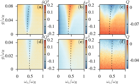
Figure S2: Nonlinearities and dissipation effects on the parametric resonances. (a), (b), (c) The same as Fig. 3 of the main text but increasing the quartic nonlinearity to $g_{4}=0.04\omega_{R}$ keeping the same decay rates. (d), (e), (f) The same as Fig. 3 but in this case the decay rates have been increased to $\kappa=\gamma=0.06\omega_{R}$ keeping the same $g_{4}$. Dashed lines are $\omega_{R}=2\bar{\omega}_{c}$.

We have checked that even for stronger nonlinearities (higher value of $g_{4}$) and/or strong dissipation the parametric resonance can still be seen so there is a resonant regime in which Raman mode fluctuations decrease in favor of cavity field amplification.

VIII Raman phonon-cavity coupling strength

Following the references Puretzky et al. (2016); Liang and Meunier (2014), Raman phonons are coupled the electric field of light $\vec{E}(x)$ through the Raman tensor R. The Hamiltonian reads

$$H=\int d^{3}x\frac{\epsilon_{0}\vec{E}(x)\cdot\underline{\underline{\epsilon}}(Q)\cdot\vec{E}(x)}{2}\approx H_{0}+\epsilon_{0}\sum_{i}\frac{\vec{E}_{i}\cdot\underline{\underline{R}}\cdot\vec{E}_{i}}{2}Q_{i},$$ (S46)

where $\epsilon_{0}$ is the vacuum permittivity and $\underline{\underline{\epsilon}}(Q)$ is the phonon-coordinate dependent polarizability tensor (dielectric tensor). Expanding linearly in the phonon coordinate $Q$ one obtains a first term $H_{0}=\int d^{3}x\frac{\epsilon_{0}\vec{E}(x)\cdot\underline{\underline{\epsilon}}(Q=0)\cdot\vec{E}(x)}{2}$ and the Raman-light coupling which is given by the second term in the right hand side of Eq. (S46). We employ the dipole approximation for the cavity mode where we assume that the electric field is constant over one unit cell and given by $\vec{E}_{i}=\frac{1}{V_{cell}}\int_{V^{i}}d^{3}x\vec{E}(x)$ where $V_{cell}$ is the volume of the unit cell and $V^{i}$ the volume of the i-th unit cell. The Raman tensor is defined as

$$R_{\alpha\beta}=V_{cell}\sum_{\mu=1}^{N}\sum_{l=1}^{3}\frac{\partial\epsilon_{\alpha\beta}}{\partial r_{l}(\mu)}\frac{e^{j}_{l}(\mu)}{\sqrt{M_{\mu}}}$$ (S47)

where $r_{l}(\mu)$ is the position of the $\mu$th atom along the direction l, $\frac{\partial\epsilon_{\alpha\beta}}{\partial r_{l}(\mu)}$ is the first derivative of the dielectric tensor over the atomic displacement, $e_{l}(\mu)$ is the displacement of the $\mu$th atom along the direction l of the Raman phonon and $M_{\mu}$ is the mass of the $\mu$th atom. Considering that the cavity mode has a constant electric field over the entire sample, $\hat{E}_{cav,i}=E_{0}\vec{e}_{c}(\hat{a}+\hat{a}^{\dagger})$, the Raman-light coupling only involves the $q=0$ phonon. Thus $\sum_{i}\hat{Q}_{i}=\sqrt{N}\hat{Q}_{q=0}=\sqrt{N}\frac{\hat{b}+\hat{b}^{\dagger}}{\sqrt{2\omega_{R}}}$, where $N=\frac{V_{samp}}{V_{cell}}$ is the total number of unit cells ($V_{samp}$ is the volume of the sample), giving rise to the coupling:

$$\frac{g}{\omega_{R}}= \frac{\epsilon_{0}E^{2}_{0}\sqrt{V_{samp}V_{cell}}}{2\omega_{R}}\tilde{R},$$ (S48)

$$\tilde{R}= \vec{e}_{c}\cdot\sum_{\mu=1}^{N}\sum_{l=1}^{3}\frac{\partial\underline{\underline{\epsilon}}}{\partial r_{l}(\mu)}\frac{e^{j}_{l}(\mu)}{\sqrt{M_{\mu}}\sqrt{2\omega_{R}}}\cdot\vec{e}_{c},$$ (S49)

where $\tilde{R}$ is the dimensionless Raman coupling and $\vec{e}_{c}$ is the polarization vector of the cavity field. Following references Puretzky et al. (2016); Liang and Meunier (2014) $\tilde{R}\sim 1-10$ for TMDs. The electric field of cavities is given by the relationship:

$$E_{0}^{2}=\frac{\omega_{c}}{\epsilon_{0}V_{eff}},$$ (S50)

where on parametric resonance $\omega_{c}=\omega_{R}/2$, leading to the final result:

$$\frac{g}{\omega_{R}}=\frac{1}{4}\tilde{R}\frac{\sqrt{V_{samp}V_{cell}}}{V_{eff}}.$$ (S51)

These arguments are rather crude and detailed research needs to be carried out for different cavity designs and Raman-active materials on a case by case basis.

References

- A. de la Torre, D. M. Kennes, M. Claassen, S. Gerber, J. W. McIver, and M. A. Sentef (2021) A. de la Torre, D. M. Kennes, M. Claassen, S. Gerber, J. W. McIver, and M. A. Sentef, “Colloquium: Nonthermal pathways to ultrafast control in quantum materials,” Rev. Mod. Phys. 93, 041002 (2021).
- Basov et al. (2017) D. N. Basov, R. D. Averitt, and D. Hsieh, “Towards properties on demand in quantum materials,” Nature Mater 16, 1077–1088 (2017).
- Bloch et al. (2022) J. Bloch, A. Cavalleri, V. Galitski, M. Hafezi, and A. Rubio, “Strongly correlated electron–photon systems,” Nature 606, 41 (2022).
- Kennes and Rubio (2023) D. M. Kennes and A. Rubio, “A New Era of Quantum Materials Mastery and Quantum Simulators In and Out of Equilibrium,” in Sketches of Physics: The Celebration Collection (Springer International Publishing, Cham, 2023) pp. 1–39.
- Nova et al. (2019) T. F. Nova, A. S. Disa, M. Fechner, and A. Cavalleri, “Metastable ferroelectricity in optically strained SrTiO3,” Science 364, 1075 (2019).
- Disa et al. (2023) A. S. Disa, J. Curtis, M. Fechner, A. Liu, A. von Hoegen, M. Först, T. F. Nova, P. Narang, A. Maljuk, A. V. Boris, B. Keimer, and A. Cavalleri, “Photo-induced high-temperature ferromagnetism in YTiO3,” Nature 617, 73 (2023).
- Siegrist et al. (2019) F. Siegrist, J. A. Gessner, M. Ossiander, C. Denker, Y. P. Chang, M. C. Schröder, A. Guggenmos, Y. Cui, J. Walowski, U. Martens, J. K. Dewhurst, U. Kleineberg, M. Münzenberg, S. Sharma, and M. Schultze, “Light-wave dynamic control of magnetism,” Nature 571, 240 (2019).
- Beaulieu et al. (2021) S. Beaulieu, S. Dong, N. Tancogne-Dejean, M. Dendzik, T. Pincelli, J. Maklar, R. Patrick Xian, M. A. Sentef, M. Wolf, A. Rubio, L. Rettig, and R. Ernstorfer, “Ultrafast dynamical Lifshitz transition,” Science Advances 7, eabd9275 (2021).
- Boström et al. (2020) E. V. Boström, M. Claassen, J. W. McIver, G. Jotzu, A. Rubio, and M. A. Sentef, “Light-induced topological magnons in two-dimensional van der Waals magnets,” SciPost Phys. 9, 061 (2020).
- Mitrano et al. (2016) M. Mitrano, A. Cantaluppi, D. Nicoletti, S. Kaiser, A. Perucchi, S. Lupi, P. Di Pietro, D. Pontiroli, M. Riccò, S. R. Clark, D. Jaksch, and A. Cavalleri, “Possible light-induced superconductivity in K3C60 at high temperature,” Nature 530, 461 (2016).
- Budden et al. (2021) M. Budden, T. Gebert, M. Buzzi, G. Jotzu, E. Wang, T. Matsuyama, G. Meier, Y. Laplace, D. Pontiroli, M. Riccò, F. Schlawin, D. Jaksch, and A. Cavalleri, “Evidence for metastable photo-induced superconductivity in K3C60,” Nat. Phys. 17, 611 (2021).
- Rowe et al. (2023) E. Rowe, B. Yuan, M. Buzzi, G. Jotzu, Y. Zhu, M. Fechner, M. Först, B. Liu, D. Pontiroli, M. Riccò, and A. Cavalleri, “Giant resonant enhancement for photo-induced superconductivity in K3C60,” (2023), 2301.08633 [cond-mat] .
- Chattopadhyay et al. (2023) S. Chattopadhyay, C. J. Eckhardt, D. M. Kennes, M. A. Sentef, D. Shin, A. Rubio, A. Cavalleri, E. A. Demler, and M. H. Michael, “Mechanisms for Long-Lived, Photo-Induced Superconductivity,” (2023), 2303.15355 [cond-mat, physics:physics] .
- von Hoegen et al. (2022) A. von Hoegen, M. Fechner, M. Först, N. Taherian, E. Rowe, A. Ribak, J. Porras, B. Keimer, M. Michael, E. Demler, and A. Cavalleri, “Amplification of Superconducting Fluctuations in Driven YBa2 Cu3 O6+x,” Phys. Rev. X 12, 031008 (2022).
- Michael et al. (2020) M. H. Michael, A. von Hoegen, M. Fechner, M. Först, A. Cavalleri, and E. Demler, “Parametric resonance of Josephson plasma waves: A theory for optically amplified interlayer superconductivity in YBa2 Cu3 O6+x,” Phys. Rev. B 102, 174505 (2020).
- McIver et al. (2020) J. W. McIver, B. Schulte, F. U. Stein, T. Matsuyama, G. Jotzu, G. Meier, and A. Cavalleri, “Light-induced anomalous Hall effect in graphene,” Nat. Phys. 16, 38 (2020).
- Kogar et al. (2020) A. Kogar, P. E. Zong, A.and Dolgirev, X. Shen, J. Straquadine, Y.Q. Bie, X. Wang, T. Rohwer, I.-C. Tung, Y. Yang, R. Li, J. Yang, S. Weathersby, S. Park, M. E. Kozina, E. J. Sie, H. Wen, P. Jarillo-Herrero, I. R. Fisher, X. Wang, and N. Gedik, “Light-induced charge density wave in LaTe3,” Nat. Phys. 16, 159 (2020).
- Dolgirev et al. (2023) P. E. Dolgirev, M. H. Michael, A. Zong, N. Gedik, and E. Demler, “Self-similar dynamics of order parameter fluctuations in pump-probe experiments,” Phys. Rev. B 101, 174306 (2023).
- Lyubarov et al. (2022) M. Lyubarov, Y. Lumer, A. Dikopoltsev, E. Lustig, Y. Sharabi, and M. Segev, “Amplified emission and lasing in photonic time crystals,” Science 377, 425 (2022).
- Michael et al. (2022) M. H. Michael, M. Först, D. Nicoletti, S. R. Ul Haque, Y. Zhang, A. Cavalleri, R. D. Averitt, D. Podolsky, and E. Demler, “Generalized Fresnel-Floquet equations for driven quantum materials,” Phys. Rev. B 105, 174301 (2022).
- Michael et al. (2023) M. H. Michael, S. R. Ul Haque, L. Windgaetter, S. Latini, Y. Zhang, A. Rubio, R. D. Averitt, and E. Demler, “Theory of time-crystalline behaviour mediated by phonon squeezing in Ta2NiSe5,” (2023), arXiv:2207.08851 [cond-mat.str-el] .
- Haque et al. (2023) S. R. Ul Haque, M. H. Michael, J. Zhu, Y. Zhang, L. Windgätter, S. Latini, J. P. Wakefield, G. F. Zhang, J. Zhang, A. Rubio, J. G. Checkelsky, E. Demler, and R. D. Averitt, “Terahertz parametric amplification as a reporter of exciton condensate dynamics,” (2023), arXiv:2304.09249 [cond-mat.str-el] .
- Dolgirev et al. (2022) P. E. Dolgirev, A. Zong, M. H. Michael, J. B. Curtis, D. Podolsky, A. Cavalleri, and E. Demler, “Periodic dynamics in superconductors induced by an impulsive optical quench,” Commun Phys 5, 1 (2022).
- Else et al. (2020) D. V. Else, C. Monroe, C. Nayak, and N. Y. Yao, “Discrete Time Crystals,” Annual Review of Condensed Matter Physics 11, 467 (2020).
- Zhang et al. (2017) J. Zhang, P. W. Hess, A. Kyprianidis, P. Becker, A. Lee, J. Smith, G. Pagano, I. D. Potirniche, A. C. Potter, A. Vishwanath, N. Y. Yao, and C. Monroe, “Observation of a discrete time crystal,” Nature 543, 217 (2017).
- Choi et al. (2017) S. Choi, J. Choi, R. Landig, G. Kucsko, H. Zhou, J. Isoya, F. Jelezko, S. Onoda, H. Sumiya, V. Khemani, C. von Keyserlingk, N. Y. Yao, E. Demler, and M. D. Lukin, “Observation of discrete time-crystalline order in a disordered dipolar many-body system,” Nature 543, 221 (2017).
- Keßler et al. (2021) H. Keßler, P. Kongkhambut, C. Georges, L. Mathey, J. G. Cosme, and A. Hemmerich, “Observation of a Dissipative Time Crystal,” Phys. Rev. Lett. 127, 043602 (2021).
- Kongkhambut et al. (2021) P. Kongkhambut, H. Keßler, J. Skulte, L. Mathey, J. G. Cosme, and A. Hemmerich, “Realization of a Periodically Driven Open Three-Level Dicke Model,” Phys. Rev. Lett. 127, 253601 (2021).
- Taheri et al. (2022) H. Taheri, A. B. Matsko, L. Maleki, and K. Sacha, “All-optical dissipative discrete time crystals,” Nature Communications 13, 848 (2022).
- Zaletel et al. (2023) M. P. Zaletel, M. Lukin, C. Monroe, C. Nayak, F. Wilczek, and N. Y. Yao, “Colloquium: Quantum and classical discrete time crystals,” Rev. Mod. Phys. 95, 031001 (2023).
- Ojeda Collado et al. (2021) H. P. Ojeda Collado, G. Usaj, C. A. Balseiro, D. H. Zanette, and J. Lorenzana, “Emergent parametric resonances and time-crystal phases in driven Bardeen-Cooper-Schrieffer systems,” Phys. Rev. Res. 3, L042023 (2021).
- Collado et al. (2023) H. P. Ojeda Collado, G. Usaj, C. A. Balseiro, D. H. Zanette, and J. Lorenzana, “Dynamical phase transitions in periodically driven Bardeen-Cooper-Schrieffer systems,” Phys. Rev. Res. 5, 023014 (2023).
- Schlawin et al. (2022) F. Schlawin, D. M. Kennes, and M. A. Sentef, “Cavity quantum materials,” Applied Physics Reviews 9 (2022).
- Curtis et al. (2023) J. B. Curtis, M. H. Michael, and E. Demler, “Local fluctuations in cavity control of ferroelectricity,” Phys. Rev. Res. 5, 043118 (2023).
- Ruggenthaler et al. (2018) M. Ruggenthaler, N. Tancogne-Dejean, J. Flick, H. Appel, and A. Rubio, “From a quantum-electrodynamical light–matter description to novel spectroscopies,” Nature Reviews Chemistry 2, 0118 (2018).
- Jarc et al. (2022) G. Jarc, S. Y. Mathengattil, F. Giusti, M. Barnaba, A. Singh, A. Montanaro, F. Glerean, E. M. Rigoni, S. D. Zilio, S. Winnerl, and D. Fausti, “Tunable cryogenic THz cavity for strong light-matter coupling in complex materials,” Review of Scientific Instruments 93, 033102 (2022).
- Appugliese et al. (2022) F. Appugliese, J. Enkner, G. L. Paravicini-Bagliani, M. Beck, C. Reichl, W. Wegscheider, G. Scalari, C. Ciuti, and J. Faist, “Breakdown of topological protection by cavity vacuum fields in the integer quantum Hall effect,” Science 375, 1030–1034 (2022).
- Lenk et al. (2022) K. Lenk, J. Li, P. Werner, and M. Eckstein, “Dynamical mean-field study of a photon-mediated ferroelectric phase transition,” Phys. Rev. B 106 (2022).
- Eckhardt et al. (2023) C. J. Eckhardt, S. Chattopadhyay, D. M. Kennes, E. A. Demler, M. A. Sentef, and M. H. Michael, “Theory of resonantly enhanced photo-induced superconductivity,” (2023), 2303.02176 [cond-mat] .
- Baydin et al. (2023) A. Baydin, M. Manjappa, S. Subhra Mishra, H. Xu, F. Tay, D. Kim, F. G. G. Hernandez, P. H. O. Rappl, E. Abramof, R. Singh, and J. Kono, “Deep-strong coupling between cavity photons and terahertz to phonons in pbte,” in CLEO 2023 (Optica Publishing Group, 2023) p. FF3D.2.
- Orgiu et al. (2015) E. Orgiu, J. George, J. A. Hutchison, E. Devaux, J. F. Dayen, B. Doudin, F. Stellacci, C. Genet, J. Schachenmayer, C. Genes, G. Pupillo, P. Samorì, and T. W. Ebbesen, “Conductivity in organic semiconductors hybridized with the vacuum field,” Nat Mater 14, 1123–1129 (2015).
- A. Thomas, E. Devaux, K. Nagarajan, T. Chervy, M. Seidel, D. Hagenmüller, S. Schütz, J. Schachenmayer, C. Genet, G. Pupillo, and T. W. Ebbesen (2019) A. Thomas, E. Devaux, K. Nagarajan, T. Chervy, M. Seidel, D. Hagenmüller, S. Schütz, J. Schachenmayer, C. Genet, G. Pupillo, and T. W. Ebbesen, “Exploring superconductivity under strong coupling with the vacuum electromagnetic field,” (2019), 1911.01459 [cond-mat, physics:quant-ph] .
- A. Thomas, E. Devaux, K. Nagarajan, G. Rogez, M. Seidel, F. Richard, C. Genet, M. Drillon, and T. W. Ebbesen (2021) A. Thomas, E. Devaux, K. Nagarajan, G. Rogez, M. Seidel, F. Richard, C. Genet, M. Drillon, and T. W. Ebbesen, “Large enhancement of ferro-magnetism under collective strong coupling of YBCO nanoparticles,” Nano Lett. 21, 4365–4370 (2021).
- Thomas et al. (2019) A. Thomas, L. Lethuillier-Karl, K. Nagarajan, R. M. A. Vergauwe, J. George, T. Chervy, A. Shalabney, E. Devaux, C. Genet, J. Moran, and T. W. Ebbesen, “Tilting a ground-state reactivity landscape by vibrational strong coupling,” Science 363, 615–619 (2019).
- Nagarajan et al. (2021) K. Nagarajan, A. Thomas, and T. W. Ebbesen, “Chemistry under vibrational strong coupling,” J. Am. Chem. Soc. 143, 16877–16889 (2021).
- Schäfer et al. (2022) C. Schäfer, J. Flick, E. Ronca, P. Narang, and A. Rubio, “Shining light on the microscopic resonant mechanism responsible for cavity-mediated chemical reactivity,” Nature Communications 13, 7817 (2022).
- Först et al. (2011) M. Först, C. Manzoni, S. Kaiser, Y. Tomioka, Y. Tokura, R. Merlin, and A. Cavalleri, “Nonlinear phononics as an ultrafast route to lattice control,” Nature Phys 7, 854–856 (2011).
- R. Matsunaga, N. Tsuji, H. Fujita, A. Sugioka, K. Makise, Y. Uzawa, H. Terai, Z. Wang, H. Aoki and R. Shimano (2014) R. Matsunaga, N. Tsuji, H. Fujita, A. Sugioka, K. Makise, Y. Uzawa, H. Terai, Z. Wang, H. Aoki and R. Shimano, “Light-induced collective pseudospin precession resonating with Higgs mode in a superconductor,” Science 345, 1145–1149 (2014).
- Buzzi et al. (2021) M. Buzzi, G. Jotzu, A. Cavalleri, J. I. Cirac, E. A. Demler, B. I. Halperin, M. D. Lukin, T. Shi, Y. Wang, and D. Podolsky, “Higgs-Mediated Optical Amplification in a Nonequilibrium Superconductor,” Phys. Rev. X 11, 011055 (2021).
- Collado et al. (2018) H. P. Ojeda Collado, J. Lorenzana, G. Usaj, and C. A. Balseiro, “Population inversion and dynamical phase transitions in a driven superconductor,” Phys. Rev. B 98, 214519 (2018).
- Juraschek et al. (2021) D. M. Juraschek, T. Neuman, J. Flick, and P. Narang, “Cavity control of nonlinear phononics,” Phys. Rev. Res. 3, L032046 (2021).
- Polkovnikov (2010) A. Polkovnikov, “Phase space representation of quantum dynamics,” Annals of Physics 325, 1790 (2010).
- Cosme et al. (2019) J. G. Cosme, J. Skulte, and L. Mathey, “Time crystals in a shaken atom-cavity system,” Phys. Rev. A 100, 053615 (2019).
- Skulte et al. (2023) J. Skulte, P. Kongkhambut, S. Rao, L. Mathey, H. Keßler, A. Hemmerich, and J. G. Cosme, “Condensate Formation in a Dark State of a Driven Atom-Cavity System,” Phys. Rev. Lett. 130, 163603 (2023).
- Basov et al. (2021) D. N. Basov, A. Asenjo-Garcia, P. J. Schuck, X. Zhu, and A. Rubio, “Polariton panorama,” Nanophotonics 10, 549 (2021).
- Kongkhambut et al. (2022) P. Kongkhambut, J. Skulte, L. Mathey, J. G. Cosme, A. Hemmerich, and H. Keßler, “Observation of a continuous time crystal,” Science 377, 670–673 (2022).
- Cardona and G.Güntherodt (1982) M. Cardona and G.Güntherodt, “Light Scattering in Solids II,” Springer-Verlag, Berlin (1982).
- Brüesch (1986) P. Brüesch, “Phonons: Theory and Experiments II,” Springer-Verlag, Berlin (1986).
- Note (1) Our calculations correspond to the quantum noise limit at zero temperature where only Stokes peaks show up. In the presence of thermal fluctuations, at finite temperature, both Stokes and Anti-stokes peaks appear in the spectrum which we present in the SI for completeness.
- Frisk Kockum et al. (2019) A. Frisk Kockum, A. Miranowicz, S. De Liberato, S. Savasta, and F. Nori, “Ultrastrong coupling between light and matter,” Nature Reviews Physics 1, 19 (2019).
- Verzhbitskiy et al. (2016) I. A. Verzhbitskiy, M. De Corato, A. Ruini, E. Molinari, A. Narita, Y. Hu, M. G. Schwab, M. Bruna, D. Yoon, S. Milana, X. Feng, K. Müllen, A. C. Ferrari, C. Casiraghi, and D. Prezzi, “Raman fingerprints of atomically precise graphene nanoribbons,” Nano Lett. 16, 3442 (2016).
- He et al. (2013) R. He, T.-F. Chung, C. Delaney, C. Keiser, L. A. Jauregui, P. M. Shand, C. C. Chancey, Y. Wang, J. Bao, and Y. P. Chen, “Observation of low energy Raman modes in twisted bilayer graphene,” Nano Lett 13, 3594 (2013).
- Valmorra et al. (2013) F. Valmorra, G. Scalari, C. Maissen, W. Fu, C. Schönenberger, J. W. Choi, H. G. Park, M. Beck, and J. Faist, “Low-Bias Active Control of Terahertz Waves by Coupling Large-Area CVD Graphene to a Terahertz metamaterial,” Nano Letters 13, 3193 (2013).
- Maissen et al. (2014) C. Maissen, G. Scalari, F. Valmorra, M. Beck, J. Faist, S. Cibella, R. Leoni, C. Reichl, C. Charpentier, and W. Wegscheider, “Ultrastrong coupling in the near field of complementary split-ring resonators,” Phys. Rev. B 90, 205309 (2014).
- Scalari et al. (2012) G. Scalari, C. Maissen, D. Turčinková, D. Hagenmüller, S. De Liberato, C. Ciuti, C. Reichl, D. Schuh, W. Wegscheider, M. Beck, and J. Faist, “Ultrastrong coupling of the cyclotron transition of a 2d electron gas to a THz metamaterial,” Science 335, 1323 (2012).
- Lin et al. (2021) K.-Q. Lin, J. Holler, J. M. Bauer, P. Parzefall, M. Scheuck, B. Peng, T. Korn, S. Bange, J. M. Lupton, and C. Schüller, “Large-Scale Mapping of Moiré Superlattices by Hyperspectral Raman Imaging,” Advanced Materials 33, 2008333 (2021).
- Puretzky et al. (2016) A. A. Puretzky, L. Liang, X. Li, K. Xiao, B. G. Sumpter, V. Meunier, and D. B. Geohegan, “Twisted MoSe2 Bilayers with Variable Local Stacking and Interlayer Coupling Revealed by Low-Frequency Raman Spectroscopy,” ACS Nano 10, 2736 (2016).
- Gunnarsson (1997) O. Gunnarsson, “Superconductivity in fullerides,” Rev. Mod. Phys. 69, 575–606 (1997).
- Goodenough (1998) J. B. Goodenough, “Jahn-Teller Phenomena In Solids,” Annual Review of Materials Science 28, 1 (1998).
- Liu et al. (2010) Y. Liu, Longxiang Zhang, M. K. Brinkley, G. Bian, T. Miller, and T.-C. Chiang, “Phonon-Induced Gaps in Graphene and Graphite Observed by Angle-Resolved Photoemission,” Phys. Rev. Lett. 105, 136804 (2010).
- V. Boström et al. (2023) E. V. Boström, A. Sriram, M. Claassen, and A. Rubio, “Controlling the magnetic state of the proximate quantum spin liquid -RuCl3 with an optical cavity,” npj Computational Materials 9, 202 (2023).
- Sandbo Chang et al. (2020) C. W. Sandbo Chang, C. Sabín, P. Forn-Díaz, F. Quijandría, A. M. Vadiraj, I. Nsanzineza, G. Johansson, and C. M. Wilson, “Observation of Three-Photon Spontaneous Parametric Down-Conversion in a Superconducting Parametric Cavity,” Phys. Rev. X 10, 011011 (2020).
- Minganti et al. (2023) F. Minganti, L. Garbe, A. Le Boité, and S. Felicetti, “Non-Gaussian superradiant transition via three-body ultrastrong coupling,” Phys. Rev. A 107, 013715 (2023).
- Breuer and Petruccione (2002) H. P. Breuer and F. Petruccione, “Open Quantum Systems,” Cambridge University Press, Cambridge, U.K. (2002).
- Landau and Lifshitz (1976) L. D. Landau and E. M. Lifshitz, “Mechanics, Course of Theoretical Physics,” Butterworth-Heinenann, Oxford, 1 (1976).
- Liang and Meunier (2014) L. Liang and V. Meunier, “First-principles Raman spectra of MoS2, WS2 and their heterostructures.” Nanoscale 6, 5394 (2014).