Forecasting Fold Bifurcations through Physics-Informed Convolutional Neural Networks

Abstract

This study proposes a physics-informed convolutional neural network (CNN) for identifying dynamical systems’ time series near a fold bifurcation. The peculiarity of this work is that the CNN is trained with a relatively small amount of data and on a single, very simple system. In contrast, the CNN is validated on much more complicated systems. A similar task requires significant extrapolation capabilities, which are obtained by exploiting physics-based information. Physics-based information is provided through a specific pre-processing of the input data, consisting mostly of a transformation into polar coordinates, normalization, transformation into the logarithmic scale, and filtering through a moving mean. The results illustrate that such data pre-processing enables the CNN to grasp the important features related to approaching a fold bifurcation, namely, the trend of the oscillation amplitude, and neglect other characteristics that are not particularly relevant, such as the vibration frequency. The developed CNN was able to correctly classify trajectories near a fold for a mass-on-moving-belt system, a van der Pol-Duffing oscillator with an attached tuned mass damper, and a pitch-and-plunge wing profile. The results obtained pave the way for the development of similar CNNs effective in real-life applications.

100

1 Introduction

Fold, or saddle-node, bifurcations are a type of bifurcation related to the merging of a saddle and a node steady-state solutions; hence the name saddle-node bifurcation [1]. The saddle and node solutions can have different natures, typically equilibrium points or periodic solutions. In both cases, if a point of each solution is represented in a plane for variations of a parameter, the branch of the two solutions generally assumes a folded shape, as shown in Fig. 1, from which the other name fold bifurcation is derived. Accordingly, fold bifurcations mark the appearance of two steady-state solutions, one stable and one unstable. In this study, we refer uniquely to fold bifurcations of periodic solutions.

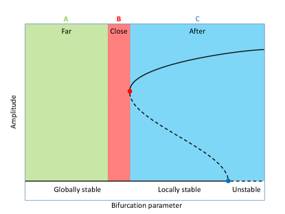
Figure 1: Illustrative example of a fold bifurcation (red dot) originated by a subcritical Andronov-Hopf bifurcation (blue dot). Green, red and blue colors mark regions far (A), close (B) and after (C) the fold, respectively.

Fold bifurcations have an important role in engineering practice. Let us consider the bifurcation scenario in Fig. 1 and assume that the upper branch of stable steady-state solutions represents the working condition of a system. If the bifurcation parameter decreases below the value of the fold bifurcation, the desired steady-state ceases to exist, leading the system to suddenly diverge from its state, usually catastrophically. Accordingly, this scenario is a mathematical catastrophe [2].

On the other hand, if the desired solution is not directly related to the fold (for instance, the trivial equilibrium in Fig. 1), then the fold does not affect the system’s local dynamics around that equilibrium. In fact, this solution does not change its stability properties when the bifurcation parameter crosses the value of the fold bifurcation. This scenario suggests that the fold bifurcation can be neglected in this case, which is often done in practice. However, the fold can have an important effect on the system’s global dynamics. Let us consider the scenario in Fig. 1, assuming that no other solution exists; in regions A and B, before the fold, the trivial solution is globally stable, while after the fold, it is only locally stable. This means that, in the locally stable region, while a small perturbation will only generate a transient effect, a large enough perturbation might lead the system to converge towards the large amplitude solutions. In practice, this scenario is particularly elusive; in fact, even after extensively testing the system, initial conditions leading to the upper branch of solutions might never be encountered, leaving the fold bifurcation undetected. However, during regular operations, it might be enough to have such perturbation only once to cause an accident. This phenomenon is usually referred to as the dynamical integrity of a stable solution, which is unbounded only for globally stable solutions [3].

Several systems of engineering relevance suffer from limited dynamical integrity and local stability. Examples include flutter instability [4, 5, 6], machining processes [7, 8], brake squeal [9, 10], robot control [11, 12], wheel shimmy [13, 14], pressure relief valves [15], turbulent flows [16, 17], electric blackouts [18, 19], human brain epilepsy [20, 21], human balance [22, 23] and prey-predator ecosystems [24, 25], to name a few.

Quite often, regions of local stability are related to subcritical bifurcations. For example, subcritical Andronov-Hopf bifurcations generate a branch of unstable periodic solutions that coexists with the stable one; subcritical Neimark-Sacker bifurcations generate a similar scenario [1], but with quasiperiodic solutions. However, in some cases, limited dynamical integrity is due to isolated branches of periodic solutions, which makes their detection even harder [26]. These are encountered in several systems, such as chemical reactors [27], traffic models [28], bridges under wind excitation [29], and shimmy of rigid wheels [30], for example.

Several methods exist to identify and predict fold bifurcations. Analytical methods typically provide an approximate solution to the system dynamics, usually in the form of a system of algebraic equations. This applies to the multiple-scale [31], averaging [32], or harmonic balance methods, to mention a few. Once a system of algebraic equations for the system’s solution is available, a fold can be found either by plotting the whole solutions in a given parameter range or by studying the system singularities through implicit derivatives of the system of algebraic equations [33]. Clearly, implementing these methods requires knowledge of the system’s equations of motion.

Numerical methods to identify fold bifurcations mostly consist of pseudo-arclength algorithms coupled with shooting techniques. By varying the bifurcation parameter, one of the two branches of periodic solutions is continued until the fold is reached [34]. Alternatively, through direct numerical integration of the equations of motion and by performing a sweep-up and a sweep-down of the bifurcation parameter, the fold is defined by a sudden jump-down and settling of the periodic solution onto an equilibrium (for a bifurcation scenario similar to the one depicted in Fig. 1). Although these methods typically exploit the system’s equations of motion, they can also be implemented through a black-box model of the system.

Similarly, experimental methods for fold bifurcation identification usually implement a sweep-up and a sweep-down of the bifurcation parameter while the system operates. The fold is identified by a sudden jump-down of a periodic solution. Additionally, control-based continuation techniques enable tracking unstable solutions until a fold is reached or even track folds in the parameter space [35].

Several methods to predict the presence of fold bifurcations directly from time series, without actually reaching it, were proposed in the literature. Suppose the system is assumed on the branch of periodic solutions leading to the fold. In that case, these methods usually exploit early-warning signals related to statistical properties of the system’s response to small perturbations [36, 19]. These methods can recognize if a system is close to a fold (in this context, usually referred to as tipping point [37] or critical transition [38, 39]), possibly enabling operators to control the system and avoid reaching the fold, which would be a non-reversible transition.

If the system in operation is on the branch of solutions not directly related to the fold, small perturbations can hardly be used to predict the fold; in fact, the fold has no local effect on the solution. However, large perturbations can still be used to forecast the fold without actually reaching it. Epureanu and coworkers developed similar methods in a series of papers [40, 4, 41]; the methods they developed allow one to predict a full bifurcation diagram from the analysis of the displacement decay of a few trajectories obtained in the pre-bifurcation scenario. A similar technique, specifically targeting fold bifurcations, was recently developed in [42] and tested experimentally in [43].

In this study, we try to perform a similar task utilizing machine learning. In particular, we utilize physics-informed convolutional neural networks (NNs). NNs have been long used to analyze time series and identify anomalies. Examples include but are not limited to, human activity recognition [44, 45], electrocardiogram classification [46, 47], speech recognition [48, 49], natural language processing [50, 51]. NNs have the ability to handle long-term dependencies and temporal context [52]. They can recognize patterns and are good at performing classifications [53]. All these properties make them a potentially useful tool for identifying if a time series is near a fold bifurcation in the parameter space. Many studies demonstrated the ability of NNs to classify and process time series related to dynamical systems. For example, they are used for chatter detection in machining [54, 55], chaos identification [56], fault detection and diagnosis in mechanical systems [57, 58], anomaly detection [59], and many other similar tasks.

Although NNs are excellent interpolators, being able to deal with large inputs, they are generally unable to extrapolate results, meaning that if an input is outside of the range of the input used for training, a NN tends to provide a wrong output [60]. One method to overcome, or at least limit, this problem is to design and train the network, taking into account the physics of the problem as well, and not only data; in other words, by providing the network with some physics-based information. Such NNs are usually referred to as physics-informed NNs. The main idea behind them is to introduce an appropriate inductive, learning, or observational bias that can steer the learning process towards identifying physically consistent solutions [61].

Inductive bias consists of tailoring the NN architecture in such a way that it implicitly satisfies some physical laws; this approach is usually implemented through some sort of invariant symmetries and rotations; this is done, for instance, by convolutional NNs [62], providing excellent results in computer vision and many other fields.

Learning bias is usually provided through the loss function, which also includes a penalty if a given mathematical function is not satisfied. This mathematical function can have any desired form, and it should represent a physical principle that we want the NN to approximately satisfy, such as, for example, conservation of mass or energy in a mechanical system [63].

Observational bias consists of providing the network with data embodying the underlying physics of the problem or using specifically designed data augmentation procedures. For instance, an observational bias can be obtained by conveniently balancing experimental and synthetic data. This method was successfully applied in a variety of fields, such as, for example, fracture propagation [64].

In this work, we investigate the ability of a physics-informed convolutional NN to identify trajectories that are close to a fold bifurcation. The NN is physics-informed through an observational bias obtained through an appropriate input normalization, which hides some signal properties (the frequency) and highlights other properties (the oscillation amplitude trend). Several studies in the literature have already approached the same problem through machine learning [65, 66]; however, up to the authors’ knowledge, it is the first time that the prediction is performed from trajectories not converging to the branch related to the fold itself. Our results show that such an NN can classify such trajectory with excellent accuracy and possesses remarkable extrapolation properties.

2 Objective

This study aims to train a convolutional NN (CNN) to identify if a time series belongs to a parameter set near a fold bifurcation. This objective is formalized in a classification task, as detailed below. The developed CNNs will be trained to distinguish between trajectories referring to a point in the parameter space that is far from a fold (region A in Fig. 1), close to a fold (region B), or after a fold (region C). Considering that the fold bifurcation generates two branches of periodic solutions, regions of the parameter space where the branches of periodic solutions do not exist are interpreted as before the fold (either far from it or close to it). In contrast, regions where they exist are considered as after.

We consider trajectories that are always initiated from relatively large initial conditions, such that they capture the transient dynamics related to the fold (although it might not be the case, as illustrated in [42]). Other methods for forecasting fold bifurcations have, in fact, the same requirement [40, 42].

The CNNs are not asked to distinguish among the region between the fold and the Andronov-Hopf bifurcation and the region after the Andronov-Hopf bifurcation. Although they are very different from an engineering perspective, their differences are qualitative only in the relative vicinity of the trivial solution, while at high amplitude, close to the stable periodic solutions, they are similar. As the time series fed to the CNNs are initiated at high amplitudes, very weak information distinguishing the two regions is available to the CNNs. Therefore, they are both classified as after. Nevertheless, this aspect is of practical relevance and will be considered in future developments of this study.

The major challenge of the study is that the CNNs will be trained on a single simple system (single-degree-of-freedom (DoF) oscillator with nonlinear damping) and tested on very different and more complicated systems. Accordingly, a CNN must discern and use the general features that characterize a system near a fold bifurcation to be effective. Conversely, all features relevant to the specific training system should be discarded. As extrapolating is notoriously hard for NNs, this task is intrinsically challenging.

The CNNs will be trained with a specific set of parameter values (except for the bifurcation parameter) of the oscillator with nonlinear damping, as described below. Then, the following test will be performed to assess the effectiveness of the network:

1. verify the accuracy in classifying time series from the same system and same range of parameter values as for the training test

2. verify the accuracy in classifying time series from the same system but a different and wider range of parameter values

3. verify the accuracy in classifying time series from other systems. In particular, three other systems are considered: a mass-on-moving-belt system, a van der Pol-Duffing oscillator with an attached dynamic vibration absorber, and a pitch-and-plunge wing profile. The systems are described in Sect. 3.

If the training data are assorted enough, the first task is achievable through any sufficiently complex NN, even a classical fully connected one. It is, in fact, a simple validation of the training. The second task already requires some sort of extrapolation from the network, but to a limited extent, considering the simplicity of the system. Conversely, the third task can be accomplished only if the network grasps the essential features of time series near fold bifurcations. Any other property specific to the training system will disturb the prediction. As shown later, this will be only possible through a proper normalization of the data provided to the network based on a physical understanding of the phenomenon.

We notice that, while the distinction between regions B and C (close and after the fold) is precisely defined by the bifurcation, the boundary between trajectories far and close to the fold is completely arbitrary. To overcome this problem, trajectories used to train the CNNs of the two groups are very well separated, as illustrated below. Then, the trained CNNs are tested on a large range of values of the bifurcation parameter in order to evaluate their capabilities.

3 Mathematical models

Four different dynamical systems are considered for the analysis: a single-DoF system with nonlinear damping, a non-smooth mass-on-moving-belt system, a van der Pol-Duffing oscillator with an attached vibration absorber, and a pitch-and-plunge wing profile. The first one is the only one used for the training.

3.1 Oscillator with nonlinear damping

A single-DoF oscillator having a nonlinear damping characteristic is considered, whose dynamics is described by the equation of motion

$$\ddot{x}+x+c_{1}\dot{x}-c_{3}\dot{x}^{3}\left(1-\dot{x}^{2}\right)=0.$$ (1)

For $c_{1}>0$, the trivial solution is always stable. For $c_{3}=0$, the system is linear, while for $c_{3}\neq 0$ the damping has a nonlinear characteristic. If $c_{3}>0$, for increasing oscillation amplitudes, first damping decreases and then increases because of the cubic and fifth order terms. As thoroughly investigated in [26], for $c_{3}=c_{3}^{*}:=40c_{1}/9$ the system presents a fold bifurcation, which generates two branches of periodic solutions existing for $c_{3}>c_{3}^{*}$. Increasing $c_{3}$, the branch of unstable periodic solutions approaches the trivial solution, reducing its dynamical integrity. However, as far as $c_{1}>0$, they never merge. The corresponding bifurcation diagram is illustrated in Fig. 2(a).

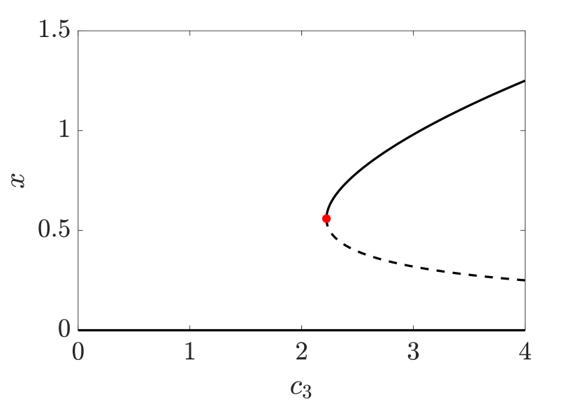
(a) Nonlinear damping system

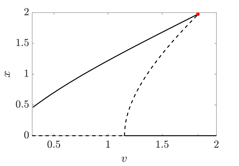
(b) Mass-on-moving-belt

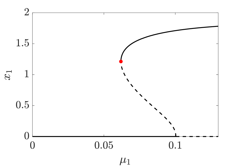
(c) Van der Pol-Duffing oscillator

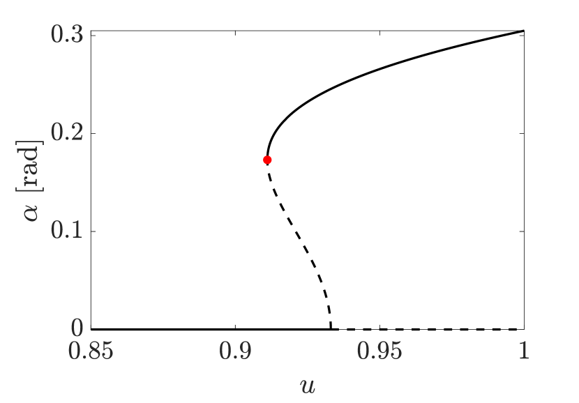
(d) Pitch-and-plunge wing

Figure 2: Bifurcation diagrams of the investigated systems; solid lines: stable solutions, dashed lines: unstable solutions; red dots: fold bifurcations. (a) System in Eq. (1) for $c_{1}=0.5$; (b) system in Eq. (2); (c) system in Eq. (5) for the parameter values $r=0.05$, $\gamma=0.97$, $\mu_{2}=0.12$ and $\alpha=0.3$; (d) system in Eq. (7).

Although the differential equation in Eq. (1) does not model any specific physical system, several mechanical systems present a nonlinear damping force, which can lead to similar dynamics.

3.2 Mass-on-moving-belt

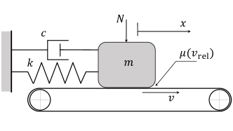
Figure 3: Mechanical model of the mass-on-moving-belt system (Eq. (2)).

We consider the classical mass-on-moving-belt system illustrated in Fig. 3. This system is an archetypal model for friction-induced vibrations [9, 10]. It is typically used for studying violin string dynamics [67] and brake squeal [68].

The non-dimensional equation of motion of the system is as follows [10]:

$$\ddot{x}+2\zeta\dot{x}+x=F_{f},$$ (2)

where

$$\left\{\begin{array}[]{ll}F_{\text{f}}=\mu\left(v_{\text{rel}}\right)&\quad v_{\text{rel}}\neq 0\\ |F_{\text{f}}|\leq\mu_{\text{s}}&\quad v_{\text{rel}}=0\end{array}\right.$$ (3)

and $\zeta$ is the damping ratio. The friction coefficient $\mu$ is given by the exponential decaying function

$$\mu(v_{\text{rel}})=\left(\mu_{\text{d}}+\left(\mu_{\text{s}}-\mu_{\text{d}}\right)\text{e}^{-\frac{|v_{\text{rel}|}}{v_{0}}}\right)\text{sign}\left(v_{\text{rel}}\right)\,,$$ (4)

where $v_{\text{rel}}=v-\dot{x}$ is the relative velocity. The friction force presents a discontinuity for $v_{\text{rel}}=0$. The adopted parameter values are $\mu_{\text{s}}=1$, $\mu_{\text{d}}=0.5$, $v_{0}=0.5$ and $\zeta=0.05$, which are the same parameter values utilized in [9, 10, 42].

For any belt velocity, the system presents an equilibrium for which the spring and the friction force are equal and opposite. However, for belt velocities $v$ larger than a specific $v_{\text{cr}}$, the equilibrium is stable, while for $v<v_{\text{cr}}$ it is unstable. The instability is marked by a subcritical Andronov-Hopf bifurcation [9]. At the Andronov-Hopf bifurcation, a branch of unstable periodic solution arises, which then merges with a branch of stable periodic solutions through a saddle-node bifurcation, as illustrated in Figure 2(b). The velocity corresponding to the saddle-node bifurcation is denoted here with $v^{*}$. For the adopted parameter values, $v_{\text{cr}}=1.151$ and $v^{*}=1.83$. The branches of stable and unstable periodic solutions merge in a non-smooth way because of the system’s discontinuity. The stable periodic solutions are characterized by a stick-slip motion.

The NNs will be asked to distinguish between trajectories for $v$ significantly larger than $v^{*}$ (far), slightly larger than $v^{*}$ (close) and smaller than $v^{*}$ (after). Testing trajectories have uniformly randomly chosen initial conditions in the range $x(0)\in\left(2,\ 3\right)$ and $\dot{x}(0)\in\left(1,\ 2\right)$.

3.3 Van der Pol-Duffing oscillator with an attached dynamic vibration absorber

The third model we consider is a van der Pol-Duffing oscillator with an attached dynamic vibration absorber. This system was thoroughly studied in the literature [69, 70], since the van der Pol oscillator is an archetypal system for self-excited oscillations [71], while the Duffing term provides a nonlinearity in the stiffness, which makes the system natural frequency amplitude-dependent [72]. Accordingly, several studies investigated the suppression and mitigation of these kinds of self-excited oscillations through dynamic vibration absorbers [73].

The equations of motion governing the system’s dynamics are

$$\mathbf{M}\ddot{\mathbf{x}}+\mathbf{C}\dot{\mathbf{x}}+\mathbf{Kx}+\mathbf{b}\left(\mathbf{x},\dot{\mathbf{x}}\right)=\mathbf{0},$$ (5)

where

$$\begin{split}&\mathbf{x}=\left[\begin{array}[]{c}x_{1}\\ x_{2}\end{array}\right],\,\mathbf{M}=\left[\begin{array}[]{cc}1&0\\ 0&r\end{array}\right],\,\mathbf{K}=\left[\begin{array}[]{cc}1+\gamma^{2}r&-\gamma^{2}r\\ -\gamma^{2}r&\gamma^{2}r\end{array}\right],\\ &\mathbf{C}=\left[\begin{array}[]{cc}-2\left(\mu_{1}+\gamma\mu_{2}r\right)&-2\gamma\mu_{2}r\\ -2\gamma\mu_{2}r&2\gamma\mu_{2}r\end{array}\right],\,\mathbf{b}=\left[\begin{array}[]{c}\alpha x_{1}^{3}+2\mu_{1}x_{1}^{2}\dot{x}_{1}\\ 0\end{array}\right].\end{split}$$ (6)

$x_{1}$ and $x_{2}$ are the state variables, respectively marking the displacement of the van der Pol-Duffing oscillator and of the vibration absorber, $r$ is the mass ratio, $\gamma$ is the natural frequency ratio, $\mu_{1}$ is the van der Pol negative damping coefficient, $\mu_{2}$ is the absorber’s pseudo damping ratio and $\alpha$ the nonlinear restoring force coefficient. For a better description of the system and the derivation of the equations of motion, we address the interested reader to [73].

For the present study we fixed parameter values at $r=0.05$, $\gamma=0.97$, $\mu_{2}=0.12$, $\alpha=0.3$, while $\mu_{1}$ is the bifurcation parameter. This set of values provides the bifurcation diagram illustrated in Fig. 2(c), which presents a fold bifurcation for $\mu_{1}^{*}=0.062$. The CNN will have to distinguish between trajectory obtained for $\mu_{1}$ significantly smaller (far), slightly smaller (close), or larger (after) than $\mu_{1}^{*}$. Testing trajectories have uniformly randomly chosen initial conditions in the range $x_{1}(0)\in\left(1,\ 2\right)$, $\dot{x}_{1}(0)\in\left(1,\ 2\right)$, $x_{2}(0)=x_{1}(0)$ and $\dot{x}_{2}(0)=0$. We note that this system presents a significant interaction between its two modes, which can make the classification of the trajectories more difficult [4, 42].

3.4 Pitch-and-plunge wing profile undergoing flutter instability

The fourth system considered is a pitch-and-plunge wing profile exposed to an airflow and undergoing flutter oscillations; the system is similar to the one studied in [74]. The pitch-and-plunge wing model considered was implemented in various previous studies [75, 76, 77] with only slight variations from the one considered here, regarding the system nonlinearities. Non-dimensional equations of motion governing the dynamics of the system are

$$\mathbf{M}\ddot{\mathbf{x}}+\mathbf{C}\dot{\mathbf{x}}+\mathbf{Kx}+\mathbf{b}\left(\mathbf{x}\right)=\mathbf{0},$$ (7)

where

$$\begin{split}&\mathbf{x}=\left[\begin{array}[]{c}y\\ \alpha\end{array}\right],\,\mathbf{K}=\left[\begin{array}[]{ccc}\Omega^{2}&\beta u^{2}\\ 0&r_{\alpha}^{2}-\nu u^{2}\end{array}\right],\,\mathbf{C}=\left[\begin{array}[]{ccc}\zeta_{h}+\beta u0\\ -\nu u&\zeta_{\alpha}\end{array}\right],\\ &\mathbf{M}=\left[\begin{array}[]{ccc}1&x_{\alpha}\\ x_{\alpha}&r_{\alpha}^{2}\end{array}\right],\,\mathbf{b}=\left[\begin{array}[]{c}0\\ \xi_{\alpha 3}\alpha^{3}+\xi_{\alpha 5}\alpha^{5}\end{array}\right],\end{split}$$ (8)

$\alpha$ marks the pitch rotation, and $y$ indicates the heave displacement, non-dimensionalized in relation to the semichord of the airfoil, while $u$ is the non-dimensional flow velocity. For the physical meaning of all the other parameters and a schematic mechanical model, we address the interested reader to [74]; a similar nomenclature is utilized here for facilitating the comparison. The adopted parameter values are $x_{\alpha}=0.2$, $r_{\alpha}=0.5$, $\beta=0.2$, $\nu=0.08$, $\Omega=0.5$, $\zeta_{\alpha}=0.01$, $\zeta_{h}=0.01$, $\xi_{\alpha 3}=-1$ and $\xi_{\alpha 5}=20$.

For the considered parameter values, the bifurcation diagram for variations of the flow velocity $u$ is shown in Figure 2(d). The equilibrium position loses stability through a subcritical Andronov-Hopf bifurcation; the emerging branch of unstable periodic solutions turns back at a fold for $u=u^{*}$ and becomes stable. For the chosen parameter values, the Andronov-Hopf bifurcation occurs at $u=0.933$, while the fold is at $u=u^{*}=0.911$. The CNN will have to classify trajectories obtained for $u$ significantly smaller (far), slightly smaller (close), or larger (after) than $u^{*}$. Testing trajectories have uniformly randomly chosen initial conditions in the range $y(0)\in\left(0.002,\ 0.01\right)$, $\dot{y}(0)\in\left(0.002,\ 0.005\right)$, $\alpha(0)\in\left(0.1,\ 0.3\right)$, and $\dot{\alpha}(0)\in\left(0.1,\ 0.3\right)$. Also, this system presents a significant coupling between pitch and plunge motions near the flutter instability, which complicates the classification of the time series [42].

4 Methods

CNNs are a particular type of machine learning architecture that has the ability to automatically extract relevant features and patterns from raw data. This ability is obtained through a series of convolutional layers that function as feature detectors. They were first introduced in the 1980s and 1990s by several researchers in the field of computer vision. One of the earliest forms of CNN is the Neocognitron, developed by Fukushima in 1980 [78], which was inspired by the structure and function of the visual cortex and was designed to recognize patterns in visual data. Another important milestone towards the development of modern CNN is represented by the LeNet-5 architecture, developed by LeCun et al. in 1998 [79], which was initially used for check recognition systems for the banking industry. Despite these developments, CNNs did not become widely adopted until the 2010s, mainly because of the lack of efficient training algorithms, regularization techniques, and the availability of larger datasets. A breakthrough in CNNs was marked by the AlexNet CNN, developed by Krizhevsky et al. [80] in 2012, which achieved a significant improvement in image classification accuracy and marked a turning point in the popularity and adoption of CNNs [53].

Today, CNNs are used in a wide range of applications, including image classification, object detection, image segmentation, natural language processing, video processing, and speech recognition. They are an obvious choice for time series classification tasks.

4.1 Convolutional neural network architecture

The CNN utilized in this study is 1D, and its key features are:

• The network is tailored to process 1-dimensional input data.

• It includes two convolutional layers. The first layer employs a filter size of 20 with 32 filters, while the second layer uses the same filter size but with 64 filters. “Causal” padding is applied to account for past values in the input sequence.

• Rectified linear units (ReLU) are used as activation functions after each convolution. Layer normalization is applied for better training stability.

• A global average pooling layer is incorporated to calculate the average value of each feature map across the entire sequence.

• A fully connected layer with neurons equal to the number of classes is employed for classification.

• The network uses a softmax layer to convert its output into class probabilities.

The network was trained using the Adam optimization algorithm with a mini-batch size of 32. Training progressed over a maximum of 50 epochs. The architecture of the CNN is represented in Fig. 4.

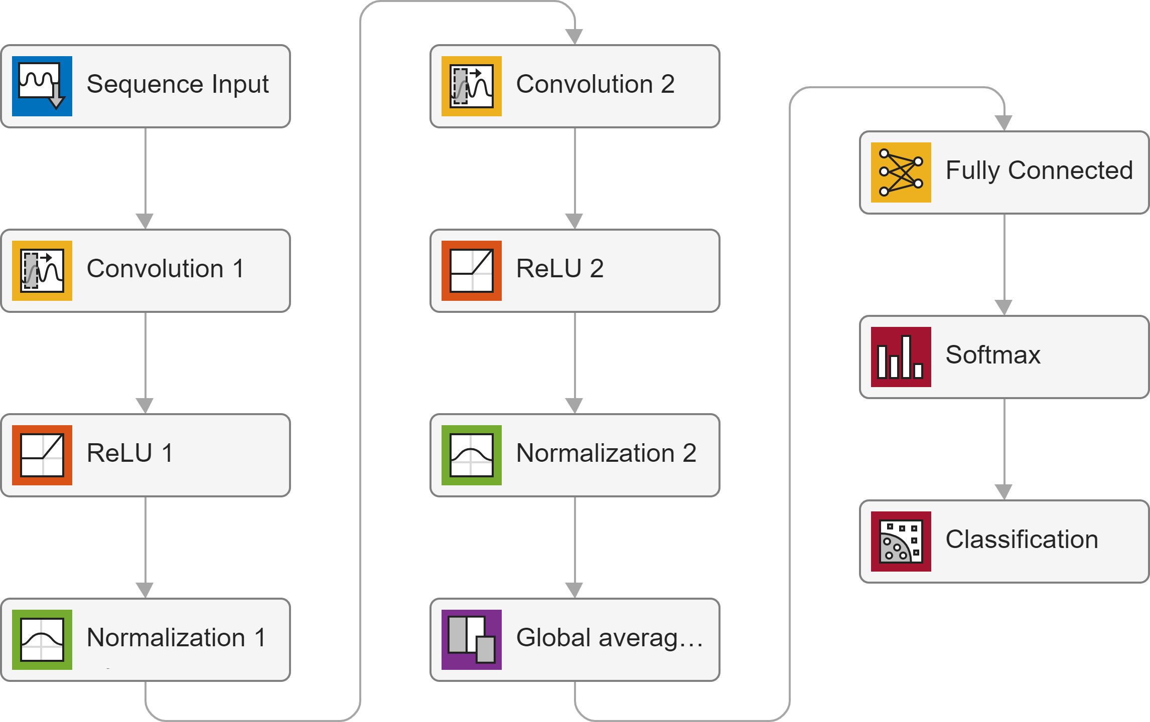
Figure 4: Graphical representation of the utilized CNN architecture.

Hyperparameters were tuned in a trial-and-error manner. However, the study does not aim to find the best possible network architecture but rather to analyze the importance of preprocessing the data through physically based assumptions, as explained in Sect. 4.2. Indeed, the same network architecture was used for all types of data normalization tested.

4.2 Physical information through input manipulation

We implemented several normalization approaches to investigate the importance of providing data in the correct form. This is an essential step for providing physical insight to the CNN and enabling extrapolation capabilities. In a recent work [42], we illustrated that time series close to a fold bifurcations dissipate energy in a particular way, which is not logarithmic as for linear systems. Conversely, energy dissipation slows down in the vicinity of the fold. This phenomenon can be understood comparing Figs. 5(a) and 5(b). By depicting the logarithmic decrement of the oscillation amplitudes and measuring its minimal value during the decay, it is possible to predict the fold bifurcation, as described in [42]. According to this procedure, the oscillation frequency can be disregarded, while only the oscillation amplitude trend is relevant. Besides, amplitude represented in a logarithmic scale better visualizes the phenomenon occurring near the fold.

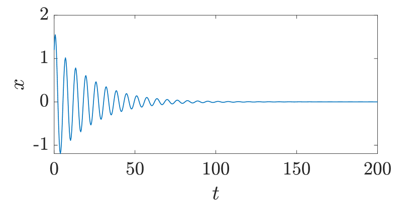
(a) Original signal - far

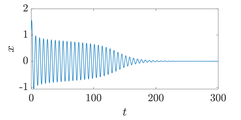
(b) Original signal - close

(c) Original signal - after

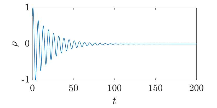
(d) Min-Max - far

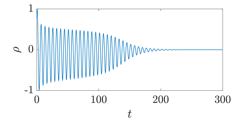
(e) Min-Max - close

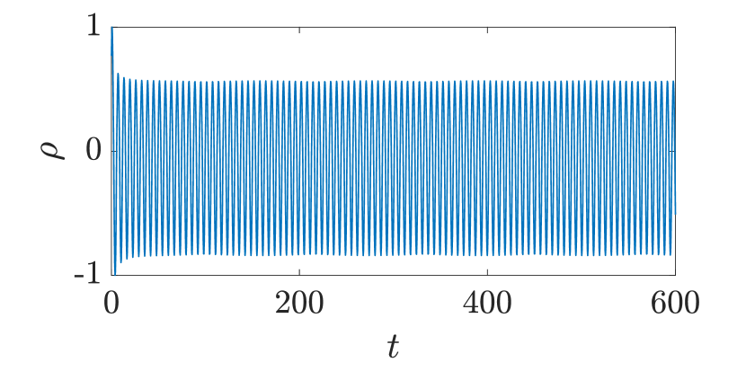
(f) Min-Max - after

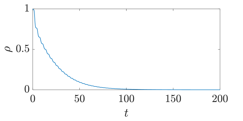
(g) Polar - far

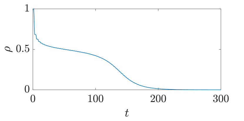
(h) Polar - close

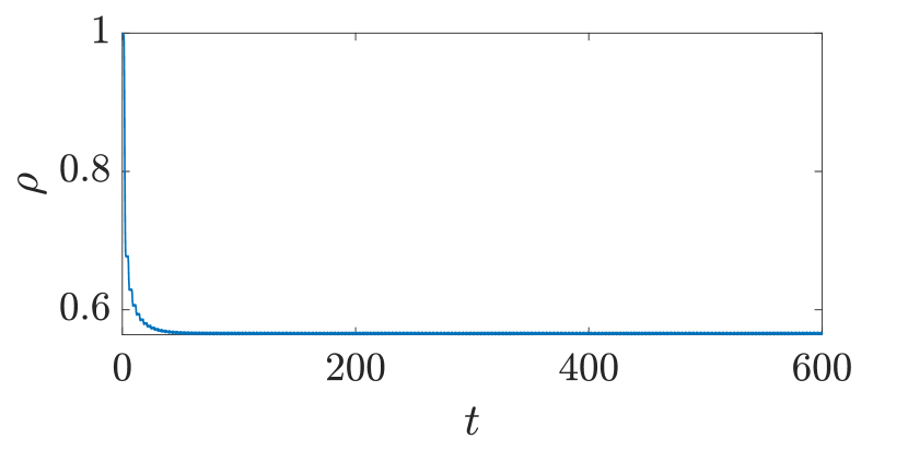
(i) Polar - after

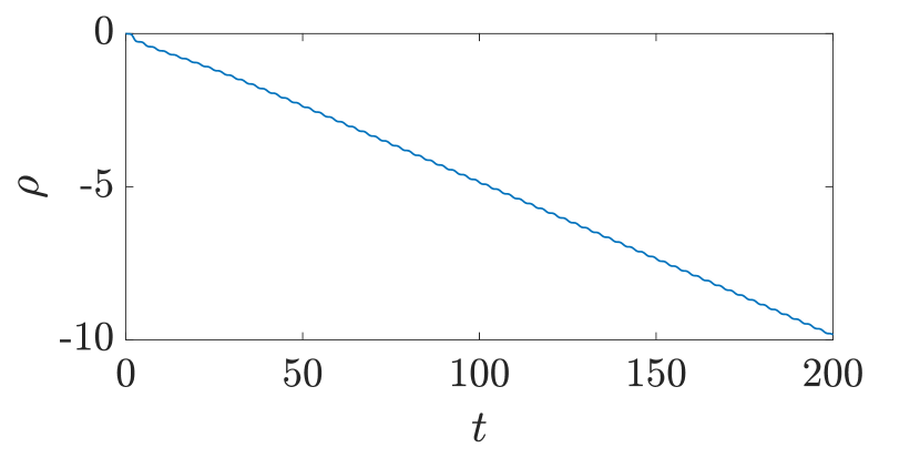
(j) Polar log - far

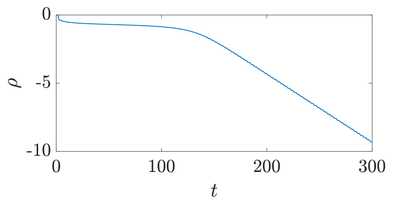
(k) Polar log - close

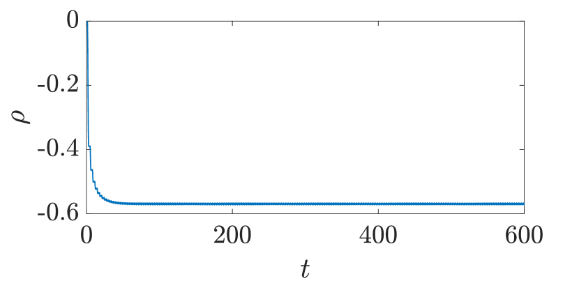
(l) Polar log - after

Figure 5: Various normalization of the signal. Left column: far from the fold, center column: close to the fold, right column: after the fold. Rows indicate, in order, the original signal, min-max normalization, transformation into polar form and normalization, transformation into polar form and logarithmic scale after normalization. Trajectories were obtained for the system in (1), with $c_{1}=0.1$, $c_{3}=0.0889$, $c_{3}=0.4222$ and $c_{3}=0.4889$; $c_{3\text{cr}}=0.444$.

In order to provide this information to the CNN, we performed various types of normalization, as described below:

1. Min-max normalization: the signal is scaled such that the largest value is 1 and the smallest one is -1, as illustrated in Figs. 5(d)-5(f). This normalization does not provide any physical insight to the CNN, but it helps deal with systems with very different amplitude ranges. It is a standard way of normalizing data and is unrelated to any physical insight of the phenomenon.

2. Polar transformation and normalization: system coordinates are transformed into polar form according to the formula $\rho=\sqrt{x^{2}+\dot{x}^{2}}$, then $\rho$ is scaled such that its maximum value is 1. The $\rho$ signal provided to the network has almost no information about the system frequency as it is not an oscillatory signal anymore. This can be beneficial as frequency is not strictly related to the vicinity of the fold bifurcation. Figures 5(g)-5(i) illustrate the transformed signals. Far from the fold (Fig. 5(g)), the signal decreases regularly until zero; close to the fold (Fig. 5(h)), it presents a sort of bump before settling to 0; after the fold (Fig. 5(i)) it rapidly converges to a constant value different from zero.

3. Polar transformation, normalization and moving mean: similar to the previous normalization, with an additional moving mean to filter high-frequency variations of the signal. The adopted moving mean has a range of 5 % of the entire signal.

4. Polar transformation, normalization and logarithmic scale: system coordinates are transformed in polar form according to the formula $\rho=\sqrt{x^{2}+\dot{x}^{2}}$, then $\rho$ is scaled such that its maximum value is 1, and finally it is transformed to a natural logarithmic scale, as illustrated in Figs. 5(j)-5(l). This normalization is similar to the previous one (without moving mean), with the additional feature that far from the bifurcation the signal is almost reduced to a straight line (it would be perfectly straight in the case of a linear single-DoF system). Besides, the signal does not converge to zero but to a negative number because of the logarithmic scale.

5. Polar transformation, normalization, logarithmic scale and moving mean: similar to the previous case, with the additional moving mean filter to eliminate high-frequency content. The adopted moving mean has a range of 5 % of the entire signal.

4.3 Training

As already mentioned, the only system used for the training was the single-DoF oscillator with nonlinear damping, whose dynamics is described by Eq. (1). 6000 time series were used for the training, 2000 for each class: far, close, and after the fold. $c_{1}$ was fixed at 0.5, leading to $c_{3}^{*}=2.22$. The value of $c_{3}$ for each class was randomly defined in the following ranges: far from the fold $c_{3}\in c_{3}^{*}\cdot(0.1,\,0.5)$, close to the fold $c_{3}\in c_{3}^{*}\cdot\left(0.9,\,0.995\right)$, and after the fold $c_{3}\in c_{3}^{*}\cdot\left(1.01,\,1.5\right)$. Initial conditions were randomly selected in the range $x(0)\in\left(0.7,\,2\right)$ and $\dot{x}(0)\in\left(0.7,\,2\right)$. All random quantities had a normal distribution within the given interval.

5 Results

The same network was trained with the same training data for all types of normalization. In all cases, 100 % accuracy was obtained during training and validation. This result suggests that the CNN utilized and the amount of data is adequate for the task. Conversely, providing correct classification for other parameter ranges is significantly more challenging. Different tests were defined, namely:

• Classify trajectories for the same system utilized during training but with $c_{1}=0.1$ instead of 0.5.

• Classify trajectories for the same system utilized during training but with $c_{1}\in\left(0.05,\ 0.7\right)$. For this task, the time series duration differs from the training data, making the system different from the one used during training from the network perspective.

• Classify trajectories for the mass-on-moving-belt system.

• Classify trajectories for the van der Pol-Duffing oscillator with an attached dynamic vibration absorber.

• Classify trajectories for the pitch-and-plunge wing profile.

For the first task, results can be quantified with a percentage of accuracy, while only qualitative assessments are given for the other tasks. Results are summarized in Table 1, while their comprehensive discussion is provided below. In the table, the following qualitative labels are provided. If far and after trajectories are significantly wrongly classified, the network is judged as “wrong”; if close trajectories are misclassified, then the label “no close” is given, if the network is overall correct, but some errors are present it is marked as “inaccurate”; while if the network provides correct classification, it is marked as “good”.

Type of normalization	Nonlinear damping $c_{1}=0.1$	Mass-on moving-belt	van der Pol -Duffing	Pitch & plunge
Min-max	66.6 %	wrong	wrong	no close
Polar	87.5 %	no close	good	good
Pol-MovMean	87.33 %	no close	good	good
Pol-log	100 %	wrong	good	inaccurate
Pol-log-MovMean	100 %	good	good	good

Table 1: Summary of the performance of the networks for different normalizations.

The table illustrates that the only network providing good results for all systems is the last one, where data were first transformed in polar coordinates, then normalized between 0 and 1, transformed in natural logarithmic scale, and finally filtered through a moving mean. However, as better detailed later, also omitting the logarithmic scale transformation but only using polar coordinates provided acceptable results, except for the mass-on-moving-belt system, possibly because of the non-smoothness of the system. Conversely, the simple min-max normalization provided very bad results; in that case, the network was completely unable to extrapolate classification capabilities to other systems. These observations clearly show that the polar transformation is the main factor for enabling the network to extrapolate results.

5.1 Min-max normalization

(a) Nonlinear damping system

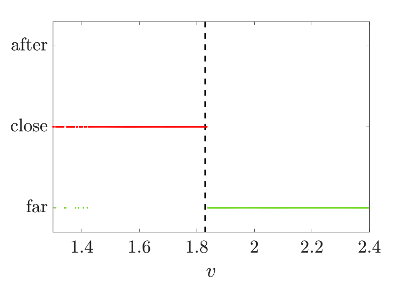
(b) Mass-on-moving-belt

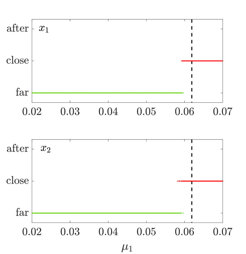
(c) Van der Pol-Duffing oscillator

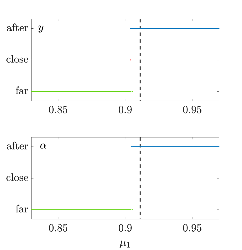
(d) Pitch-and-plunge wing

Figure 6: Prediction diagrams obtained by the CNN trained with min-max normalized data. Color interpretation: green-far, red-close, blue-after.

The network trained with simply normalized data was completely unable to extrapolate classification capabilities. Although it obtained a 100 % accuracy in the validation set, simple variations of the $c_{1}$ parameter prevented it from providing meaningful results (Fig. 6(a)). Regarding other systems investigated, prediction was always inadequate; we note that far trajectories were generally correctly classified, while after and close trajectories were often systematically confused with each other (Fig. 6). Considering the simple normalization provided, this poor result is not surprising.

5.2 Polar transformation and normalization

(a) Nonlinear damping system

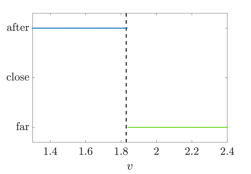
(b) Mass-on-moving-belt

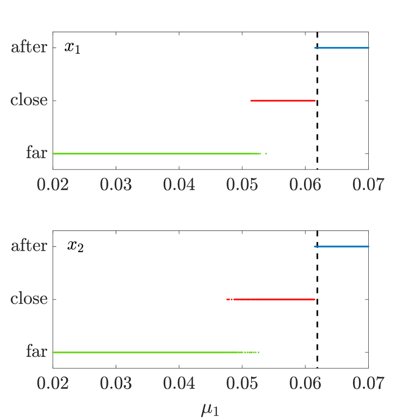
(c) Van der Pol-Duffing oscillator

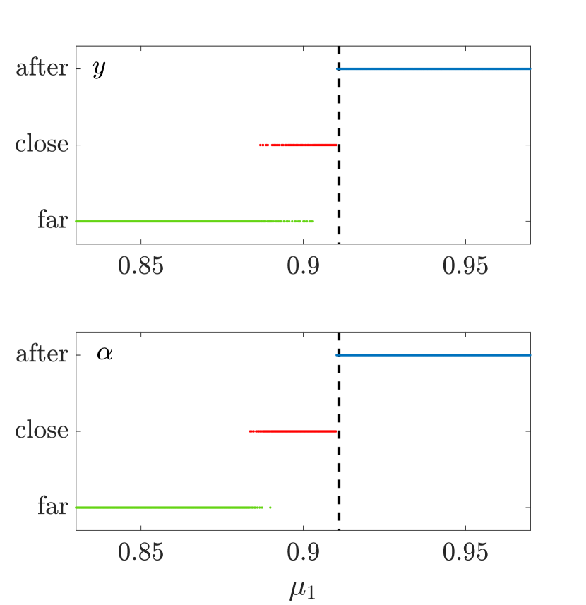
(d) Pitch-and-plunge wing

Figure 7: Prediction diagrams obtained by the CNN trained with data normalized in polar form. Color interpretation: green-far, red-close, blue-after.

The polar form transformation and amplitude normalization between 0 and 1 provided much better results. This is mostly due to the almost complete elimination of the frequency of oscillation from the data, which is not related to general traits of system approaching a fold bifurcation. We also note that the network never misclassified far and after trajectories. Regarding the system with nonlinear damping (Fig. 7(a)), reducing $c_{1}$ the network significantly reduced the trajectories classified as close, which are limited to those extremely close to the fold. About the mass-on-moving-belt system (Fig. 7(b)), the network completely overlooked close trajectories, which were always classified as far. Regarding the van der Pol-Duffing oscillator (Fig. 7(c)) and the pitch-and-plunge wing profile (Fig. 7(d)) the classification was excellent with both degrees of freedom.

5.3 Polar transformation, normalization and moving mean filter

(a) Nonlinear damping system

(b) Mass-on-moving-belt

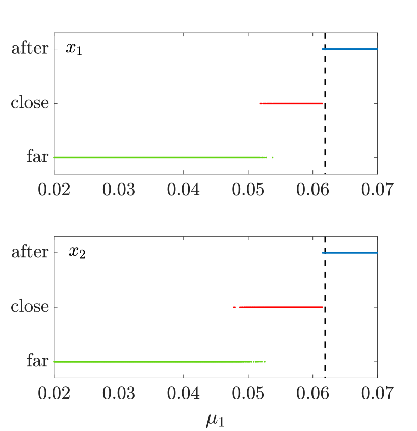
(c) Van der Pol-Duffing oscillator

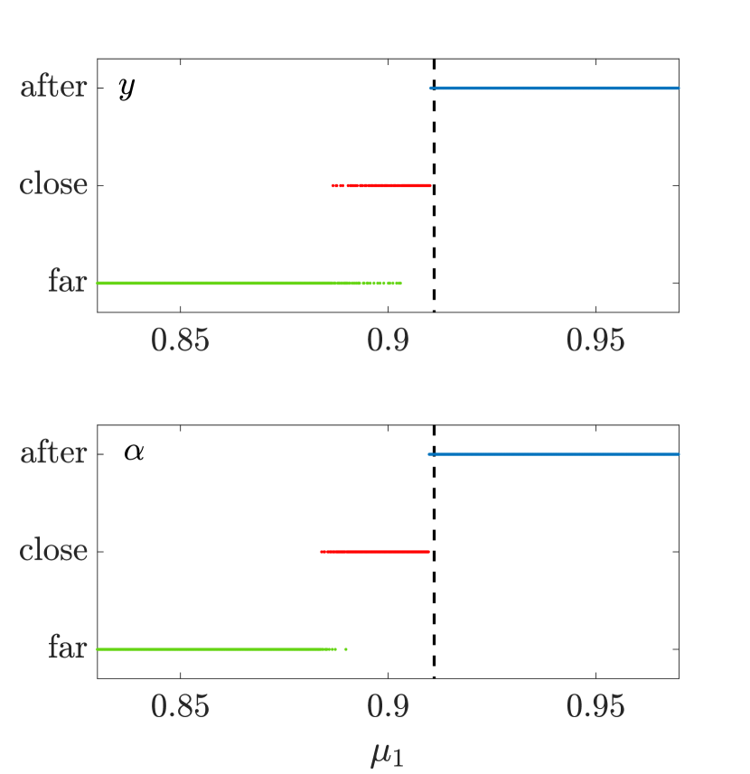
(d) Pitch-and-plunge wing

Figure 8: Prediction diagrams obtained by the CNN trained with data normalized in polar form filtered with a moving mean. Color interpretation: green-far, red-close, blue-after.

Adding a moving mean filter to the previous case (polar transformation and normalization) did not provide any advantage. This network provided practically the same results as the previous one. Namely, acceptable results for the nonlinear damping oscillator (Fig. 8(a)), missed close trajectories in the mass-on-moving-belt system (Fig. 8(b)), excellent results for the van der Pol-Duffing oscillator (Fig. 8(c)) and pith-and-plunge wing (Fig. 8(d)). Indeed, this is not surprising considering that the CNN already includes filters that can provide a similar effect as the moving mean filter. However, this is not always the case, as shown in Sect. 5.5.

5.4 Polar transformation, normalization and logarithmic scale

(a) Nonlinear damping system

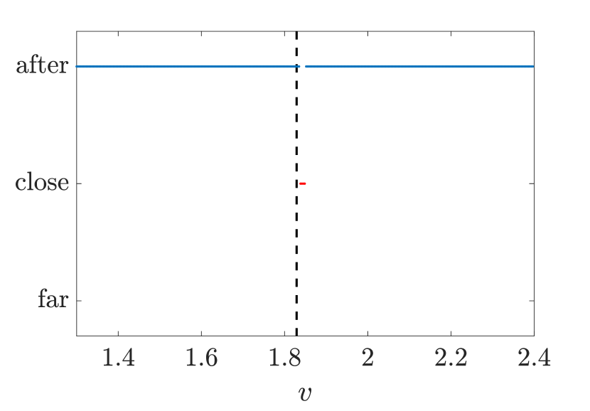
(b) Mass-on-moving-belt

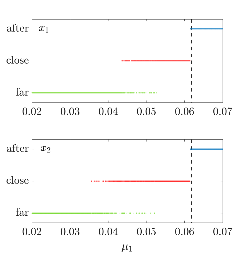
(c) Van der Pol-Duffing oscillator

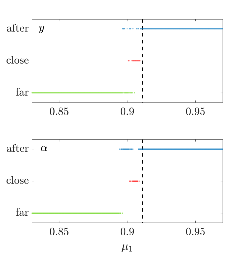
(d) Pitch-and-plunge wing

Figure 9: Prediction diagrams obtained by the CNN trained with data normalized in polar form and in logarithmic scale. Color interpretation: green-far, red-close, blue-after.

The transformation into a logarithmic scale reflects the observation that the decrement of the oscillation amplitude is logarithmic in a linear system. Accordingly, if far from the bifurcation the nonlinearities are weak, the amplitude is expected to decrease approximately logarithmically (of course, modal interaction modifies this behavior), which in a logarithmic scale appears linear. Training the network with data in polar coordinates, normalized and scaled in logarithmic coordinates provided better results than seen in the previous case for the nonlinearly damped oscillator (Fig. 9(a)), which were excellent for all the investigated range of $c_{1}$. However, the network provided a completely wrong classification for the mass-on-moving-belt system (Fig. 9(b)); for this system, all far cases were incorrectly classified as after. Interestingly, some close trajectories were correctly classified. It is hard to explain understand the mechanism leading to such a wrong classification. Regarding the van der Pol-Duffing oscillator (Fig. 9(c)), the network performed well; in this case, the region of close trajectories was much larger than for the networks whose data were not in logarithmic scale (Figs. 7(c) and 8(c)); the prediction based on the primary system displacement ($x_{1}$) provided a smaller close region than if based on the vibration absorber displacement ($x_{2}$). About the pitch-and-plunge wing profile, the classification is acceptable; however, some trajectories in the close region were mistakenly classified as after; this problem is less significant if classification is based on plunge motion ($y$), rather than pitch ($\alpha$).

5.5 Polar transformation, normalization, logarithmic scale and moving mean

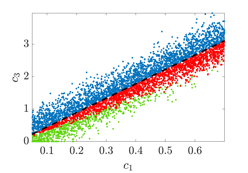
(a) Nonlinear damping system

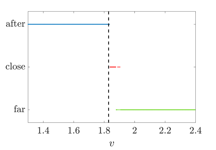
(b) Mass-on-moving-belt

(c) Van der Pol-Duffing oscillator

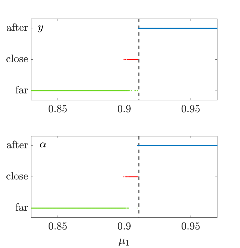
(d) Pitch-and-plunge wing

Figure 10: Prediction diagrams obtained by the CNN trained with data normalized in polar form and logarithmic scale and then filtered with a moving mean. Color interpretation: green-far, red-close, blue-after.

The last case we consider is similar to the previous one, with an additional moving mean filter applied to the data to remove variations of the amplitude in polar coordinates during each complete oscillation. The same filter was applied for the case not in logarithmic scale and produced no improvement (see Sect. 5.3). Conversely, in this case, it significantly enhanced the accuracy of the network. All tested cases provided very good results. In particular, trajectories of the nonlinearly damped oscillator were correctly classified for all the investigated range of $c_{1}$ (Fig. 10(a)). Excellent classification was also provided for the mass-on-moving-belt system (Fig. 10(b)); we remark that this was the only normalization that enabled the network to correctly classify close trajectories for this system. The network was able to correctly distinguish between the three classes also for the van der Pol-Duffing oscillator (Fig. 10(c)) and pitch-and-plunge wing (Fig. 10(d)), using any of the coordinates.

6 Discussion and conclusions

The performed analysis demonstrates that a properly trained neural network can recognize a trajectory passing close to a fold bifurcation. However, in order for the network to capture the important features of such trajectories and provide correct classification for different systems, it is essential that training data are properly normalized. This step eliminates inessential information from the data, such as oscillation frequency, allowing the network to focus on important ones, like the decrement of oscillation amplitude. The results obtained with this method are remarkable. In fact, a network trained with a single, very simple system performed very well on three different mathematical systems modeling mechanical systems of engineering relevance, thus exhibiting excellent extrapolation capabilities. The most important step of the normalization was the transformation in polar coordinates, which eliminates almost completely information about oscillation frequency, thus highlighting amplitude. Applying a logarithmic scaling, providing a physically more relevant scale, further improved the network performance. Finally, introducing a moving mean filter and eliminating any residual information about variations in single oscillation periods enhanced even more correct classification capabilities. The moving mean could also eliminate noise in the data, an aspect not investigated in the present study. Every step of data normalization is related to the physical understanding of the problem, and it is not standard for signal processing, except for the moving mean.

The present analysis does not rule out that a classical data normalization (with no physical basis) is sufficient for an NN to classify trajectories in different systems. However, it most probably requires that the training data involves several systems.

We note that there is a significant overlap in the region where trajectories are classified as either far or close (particularly for the van der Pol-Duffing oscillator). This is mostly because some initial conditions lead to a dynamical behavior almost unaffected by the fold, while other initial conditions generate trajectories more distorted by it. This phenomenon was clearly illustrated in [42].

Regarding the limitations of the approach, we remark that the range of the initial conditions significantly affects the network’s accuracy. In fact, referring to the best-performing case, the network has to distinguish between scenarios similar to those in Figs. 5(j) and 5(k); Fig. 5(k) might be distorted if large initial conditions move down the bump, confusing the CNN.

Additionally, we note that in the studied cases, the simulations were run until the systems reached extremely small oscillation amplitudes (about $e^{-10}$, see Fig. 5(j)). In the case of a real system, and in the presence of noise, it is unreasonable to expect the system to reach such small amplitudes, which would modify the numerical values in the far and close cases, potentially generating wrong classifications. In particular, far and close trajectories might be classified as after.

These potential limitations can be overcome by increasing the heterogeneity of training data, for example, by adding noise and considering different systems. Another way to solve the issues is to use a sliding window convolutional neural network, which would analyze the signal by dividing it in time window frames. This way, the network would provide a list of outputs for each signal. This output list could then be further analyzed to obtain a single classification output.

This study does not investigate other machine learning algorithms which might provide similar or better results. For instance, a random forests architecture might also lead to good results. Alternatively, two autoencoders could be trained, one on far and one on after trajectories, in order to identify close ones. Additionally, the convolutional layers utilized are relatively standard and not specifically designed for the accomplished task. A thorough analysis of the hyperparameters and alternative network architectures might provide significant improvement.

In the analysis, training data was relatively little and purposely limited to a single simple system. However, training the network with more data obtained from diverse systems, including experimental ones, might enable it to correctly classify trajectories also in real-life problems.

At last, we note that this study is limited in its scope, as the network only distinguishes between trajectories far, close, or after the fold and does not try to estimate the position of the fold, as other deterministic methods do [40, 42]. While training the network to identify the position of the fold based on some time series computed before the fold is probably very challenging, it is likely feasible to add more classes to distinguish, for example, between close and very close. Additionally, including trajectories starting at lower amplitude, it might be possible to distinguish also between trajectories far from, close to, or after the Andronov-Hopf bifurcation (if present). However, these further developments probably require more diverse and abundant training data.

In general, we think that this study paves the way for the development of an algorithm for fold bifurcation prediction applicable in real-life problems, which might represent a useful tool in engineering, especially for safety monitoring of dynamical systems.

Data availability

The code utilized for generating the results presented in the paper is publicly available at https://gdrg.mm.bme.hu.

Funding

The research reported in this paper has been supported by Project no. TKP-6-6/PALY-2021 provided by the Ministry of Culture and Innovation of Hungary from the National Research, Development and Innovation Fund, financed under the TKP2021-NVA funding scheme and by the National Research, Development and Innovation Office (Grant no. NKFI-134496).

References

- [1] Y. A. Kuznetsov, I. A. Kuznetsov, Y. Kuznetsov, Elements of applied bifurcation theory, Vol. 112, Springer, 1998.
- [2] V. I. Arnol’d, Singularity theory, Vol. 53, Cambridge University Press, 1981.
- [3] S. Lenci, G. Rega, et al., Global Nonlinear Dynamics for Engineering Design and System Safety, Vol. 588, Springer, 2019.
- [4] A. Ghadami, B. I. Epureanu, Bifurcation forecasting for large dimensional oscillatory systems: forecasting flutter using gust responses, Journal of Computational and Nonlinear Dynamics 11 (6) (2016) 061009.
- [5] A. Nitti, M. Stender, N. Hoffmann, A. Papangelo, Spatially localized vibrations in a rotor subjected to flutter, Nonlinear Dynamics 103 (2021) 309–325.
- [6] G. Habib, Dynamical integrity assessment of stable equilibria: a new rapid iterative procedure, Nonlinear Dynamics 106 (3) (2021) 2073–2096.
- [7] Z. Dombovari, A. Iglesias, T. G. Molnar, G. Habib, J. Munoa, R. Kuske, G. Stepan, Experimental observations on unsafe zones in milling processes, Philosophical Transactions of the Royal Society A 377 (2153) (2019) 20180125.
- [8] B. Szaksz, G. Stepan, G. Habib, Dynamical integrity estimation in time delayed systems: a rapid iterative algorithm, Journal of Sound and Vibration 571 (2024) 118045.
- [9] A. Papangelo, M. Ciavarella, N. Hoffmann, Subcritical bifurcation in a self-excited single-degree-of-freedom system with velocity weakening–strengthening friction law: analytical results and comparison with experiments, Nonlinear dynamics 90 (2017) 2037–2046.
- [10] J. L. Hu, G. Habib, Friction-induced vibration suppression via the tuned mass damper: optimal tuning strategy, Lubricants 8 (11) (2020) 100.
- [11] G. Habib, G. Rega, G. Stepan, Nonlinear bifurcation analysis of a single-dof model of a robotic arm subject to digital position control, Journal of Computational and Nonlinear Dynamics 8 (1) (2013) 011009.
- [12] G. Habib, A. Bártfai, A. Barrios, Z. Dombovari, Bistability and delayed acceleration feedback control analytical study of collocated and non-collocated cases, Nonlinear Dynamics 108 (3) (2022) 2075–2096.
- [13] H. Z. Horvath, D. Takacs, Stability and local bifurcation analyses of two-wheeled trailers considering the nonlinear coupling between lateral and vertical motions, Nonlinear Dynamics (2022) 1–18.
- [14] G. Habib, A. Epasto, Towed wheel shimmy suppression through a nonlinear tuned vibration absorber, Nonlinear Dynamics 111 (10) (2023) 8973–8986.
- [15] F. Kadar, G. Stepan, Nonlinear dynamics and safety aspects of pressure relief valves, Nonlinear Dynamics (2023) 1–16.
- [16] S. Cherubini, P. De Palma, J.-C. Robinet, Nonlinear optimals in the asymptotic suction boundary layer: Transition thresholds and symmetry breaking, Physics of Fluids 27 (3).
- [17] R. Kerswell, Nonlinear nonmodal stability theory, Annual Review of Fluid Mechanics 50 (2018) 319–345.
- [18] A. Gajduk, M. Todorovski, L. Kocarev, Stability of power grids: An overview, The European Physical Journal Special Topics 223 (12) (2014) 2387–2409.
- [19] H. Ren, D. Watts, Early warning signals for critical transitions in power systems, Electric power systems research 124 (2015) 173–180.
- [20] P. Suffczynski, S. Kalitzin, F. L. Da Silva, Dynamics of non-convulsive epileptic phenomena modeled by a bistable neuronal network, Neuroscience 126 (2) (2004) 467–484.
- [21] W. W. Lytton, Computer modelling of epilepsy, Nature Reviews Neuroscience 9 (8) (2008) 626–637.
- [22] M. S. Zakynthinaki, J. R. Stirling, C. A. Cordente Martínez, A. L. Díaz de Durana, M. S. Quintana, G. R. Romo, J. S. Molinuevo, Modeling the basin of attraction as a two-dimensional manifold from experimental data: Applications to balance in humans, Chaos: An Interdisciplinary Journal of Nonlinear Science 20 (1).
- [23] V. A. Smith, T. E. Lockhart, M. L. Spano, Basins of attraction in human balance, The European Physical Journal Special Topics 226 (2017) 3315–3324.
- [24] K. Saleh, Basins of attraction in a modified ratio-dependent predator-prey model with prey refugee, AIMS Mathematics 7 (8) (2022) 14875–14894.
- [25] S. Garai, S. Karmakar, S. Jafari, N. Pal, Coexistence of triple, quadruple attractors and wada basin boundaries in a predator–prey model with additional food for predators, Communications in Nonlinear Science and Numerical Simulation 121 (2023) 107208.
- [26] G. Habib, G. I. Cirillo, G. Kerschen, Isolated resonances and nonlinear damping, Nonlinear Dynamics 93 (2018) 979–994.
- [27] A. Uppal, W. Ray, A. Poore, The classification of the dynamic behavior of continuous stirred tank reactors–influence of reactor residence time, Chemical Engineering Science 31 (3) (1976) 205–214.
- [28] K. Martinovich, A. K. Kiss, Nonlinear effects of saturation in the car-following model, Nonlinear Dynamics 111 (3) (2023) 2555–2569.
- [29] D. Zulli, A. Luongo, Bifurcation and stability of a two-tower system under wind-induced parametric, external and self-excitation, Journal of Sound and Vibration 331 (2) (2012) 365–383.
- [30] D. Takács, G. Stépán, S. J. Hogan, Isolated large amplitude periodic motions of towed rigid wheels, Nonlinear Dynamics 52 (2008) 27–34.
- [31] A. H. Nayfeh, D. T. Mook, Nonlinear oscillations, John Wiley & Sons, 2008.
- [32] F. Verhulst, A Toolbox of Averaging Theorems: Ordinary and Partial Differential Equations, Vol. 12, Springer Nature, 2023.
- [33] M. Golubitsky, D. G. Schaeffer, Singularities and Groups in Bifurcation Theory: Volume I, Vol. 1, Springer, New York, 1985.
- [34] A. H. Nayfeh, B. Balachandran, Applied nonlinear dynamics: analytical, computational, and experimental methods, John Wiley & Sons, 2008.
- [35] L. Renson, J. Sieber, D. A. Barton, A. Shaw, S. Neild, Numerical continuation in nonlinear experiments using local gaussian process regression, Nonlinear Dynamics 98 (2019) 2811–2826.
- [36] R. Liu, P. Chen, K. Aihara, L. Chen, Identifying early-warning signals of critical transitions with strong noise by dynamical network markers, Scientific reports 5 (1) (2015) 17501.
- [37] T. M. Lenton, Tipping positive change, Philosophical Transactions of the Royal Society B 375 (1794) (2020) 20190123.
- [38] M. Scheffer, J. Bascompte, W. A. Brock, V. Brovkin, S. R. Carpenter, V. Dakos, H. Held, E. H. Van Nes, M. Rietkerk, G. Sugihara, Early-warning signals for critical transitions, Nature 461 (7260) (2009) 53–59.
- [39] S. J. Lade, T. Gross, Early warning signals for critical transitions: a generalized modeling approach, PLoS computational biology 8 (2) (2012) e1002360.
- [40] J. Lim, B. I. Epureanu, Forecasting a class of bifurcations: Theory and experiment, Physical Review E 83 (1) (2011) 016203.
- [41] S. Chen, B. Epureanu, Forecasting bifurcations of multi-degree-of-freedom nonlinear systems with parametric resonance, Nonlinear Dynamics 93 (2018) 63–78.
- [42] G. Habib, Predicting saddle-node bifurcations using transient dynamics: A model-free approach, Nonlinear Dynamics.
- [43] F. Kadar, G. Stepan, G. Habib, Model-free fold bifurcation prediction from pre-bifurcation scenario: experimental validation through wheel shimmy vibrations, Under review.
- [44] F. J. Ordóñez, D. Roggen, Deep convolutional and LSTM recurrent neural networks for multimodal wearable activity recognition, Sensors 16 (1) (2016) 115.
- [45] C. Xu, D. Chai, J. He, X. Zhang, S. Duan, Innohar: A deep neural network for complex human activity recognition, Ieee Access 7 (2019) 9893–9902.
- [46] M. Zihlmann, D. Perekrestenko, M. Tschannen, Convolutional recurrent neural networks for electrocardiogram classification, in: 2017 Computing in Cardiology (CinC), IEEE, 2017, pp. 1–4.
- [47] A. Y. Hannun, P. Rajpurkar, M. Haghpanahi, G. H. Tison, C. Bourn, M. P. Turakhia, A. Y. Ng, Cardiologist-level arrhythmia detection and classification in ambulatory electrocardiograms using a deep neural network, Nature medicine 25 (1) (2019) 65–69.
- [48] G. Hinton, L. Deng, D. Yu, G. E. Dahl, A.-r. Mohamed, N. Jaitly, A. Senior, V. Vanhoucke, P. Nguyen, T. N. Sainath, et al., Deep neural networks for acoustic modeling in speech recognition: The shared views of four research groups, IEEE Signal processing magazine 29 (6) (2012) 82–97.
- [49] A. B. Nassif, I. Shahin, I. Attili, M. Azzeh, K. Shaalan, Speech recognition using deep neural networks: A systematic review, IEEE access 7 (2019) 19143–19165.
- [50] Y. Goldberg, A primer on neural network models for natural language processing, Journal of Artificial Intelligence Research 57 (2016) 345–420.
- [51] Y. Goldberg, Neural network methods for natural language processing, Springer Nature, 2022.
- [52] Y. Yu, X. Si, C. Hu, J. Zhang, A review of recurrent neural networks: Lstm cells and network architectures, Neural computation 31 (7) (2019) 1235–1270.
- [53] Z. Li, F. Liu, W. Yang, S. Peng, J. Zhou, A survey of convolutional neural networks: analysis, applications, and prospects, IEEE transactions on neural networks and learning systems.
- [54] M. Lamraoui, M. Barakat, M. Thomas, M. E. Badaoui, Chatter detection in milling machines by neural network classification and feature selection, Journal of Vibration and Control 21 (7) (2015) 1251–1266.
- [55] M. H. Rahimi, H. N. Huynh, Y. Altintas, On-line chatter detection in milling with hybrid machine learning and physics-based model, CIRP Journal of Manufacturing Science and Technology 35 (2021) 25–40.
- [56] N. Boullé, V. Dallas, Y. Nakatsukasa, D. Samaddar, Classification of chaotic time series with deep learning, Physica D: Nonlinear Phenomena 403 (2020) 132261.
- [57] H. Chen, Z. Chai, O. Dogru, B. Jiang, B. Huang, Data-driven designs of fault detection systems via neural network-aided learning, IEEE Transactions on Neural Networks and Learning Systems 33 (10) (2021) 5694–5705.
- [58] R. F. R. Junior, I. A. dos Santos Areias, M. M. Campos, C. E. Teixeira, L. E. B. da Silva, G. F. Gomes, Fault detection and diagnosis in electric motors using 1d convolutional neural networks with multi-channel vibration signals, Measurement 190 (2022) 110759.
- [59] Z. Li, J. Li, Y. Wang, K. Wang, A deep learning approach for anomaly detection based on sae and lstm in mechanical equipment, The International Journal of Advanced Manufacturing Technology 103 (2019) 499–510.
- [60] M. Zhu, H. Zhang, A. Jiao, G. E. Karniadakis, L. Lu, Reliable extrapolation of deep neural operators informed by physics or sparse observations, Computer Methods in Applied Mechanics and Engineering 412 (2023) 116064.
- [61] G. E. Karniadakis, I. G. Kevrekidis, L. Lu, P. Perdikaris, S. Wang, L. Yang, Physics-informed machine learning, Nature Reviews Physics 3 (6) (2021) 422–440.
- [62] Y. LeCun, Y. Bengio, et al., Convolutional networks for images, speech, and time series, The handbook of brain theory and neural networks 3361 (10) (1995) 1995.
- [63] M. Raissi, P. Perdikaris, G. E. Karniadakis, Physics-informed neural networks: A deep learning framework for solving forward and inverse problems involving nonlinear partial differential equations, Journal of Computational physics 378 (2019) 686–707.
- [64] D. Chen, Y. Li, K. Liu, Y. Li, A physics-informed neural network approach to fatigue life prediction using small quantity of samples, International Journal of Fatigue 166 (2023) 107270.
- [65] T. M. Bury, R. Sujith, I. Pavithran, M. Scheffer, T. M. Lenton, M. Anand, C. T. Bauch, Deep learning for early warning signals of tipping points, Proceedings of the National Academy of Sciences 118 (39) (2021) e2106140118.
- [66] D. Patel, E. Ott, Using machine learning to anticipate tipping points and extrapolate to post-tipping dynamics of non-stationary dynamical systems, Chaos: An Interdisciplinary Journal of Nonlinear Science 33 (2).
- [67] R. Leine, D. Van Campen, A. De Kraker, L. Van Den Steen, Stick-slip vibrations induced by alternate friction models, Nonlinear dynamics 16 (1998) 41–54.
- [68] N. Kinkaid, O. M. O’Reilly, P. Papadopoulos, Automotive disc brake squeal, Journal of sound and vibration 267 (1) (2003) 105–166.
- [69] V. Gattulli, F. Di Fabio, A. Luongo, Simple and double hopf bifurcations in aeroelastic oscillators with tuned mass dampers, Journal of the Franklin Institute 338 (2-3) (2001) 187–201.
- [70] V. Gattulli, F. Di Fabio, A. Luongo, One to one resonant double hopf bifurcation in aeroelastic oscillators with tuned mass dampers, Journal of Sound and Vibration 262 (2) (2003) 201–217.
- [71] M. R. Cândido, J. Llibre, C. Valls, Non-existence, existence, and uniqueness of limit cycles for a generalization of the van der pol–duffing and the rayleigh–duffing oscillators, Physica D: Nonlinear Phenomena 407 (2020) 132458.
- [72] I. Kovacic, M. J. Brennan, The Duffing equation: nonlinear oscillators and their behaviour, John Wiley & Sons, 2011.
- [73] G. Habib, G. Kerschen, Suppression of limit cycle oscillations using the nonlinear tuned vibration absorber, Proceedings of the Royal Society A: Mathematical, Physical and Engineering Sciences 471 (2176) (2015) 20140976.
- [74] A. Malher, C. Touzé, O. Doaré, G. Habib, G. Kerschen, Flutter control of a two-degrees-of-freedom airfoil using a nonlinear tuned vibration absorber, Journal of Computational and Nonlinear Dynamics 12 (5) (2017) 051016.
- [75] E. H. Dowell, A modern course in aeroelasticity, Vol. 217, Springer, 2014.
- [76] Y. S. Lee, A. F. Vakakis, L. A. Bergman, D. M. McFarland, G. Kerschen, Suppressing aeroelastic instability using broadband passive targeted energy transfers, part 1: Theory, AIAA journal 45 (3) (2007) 693–711.
- [77] Y. S. Lee, G. Kerschen, D. M. McFarland, W. J. Hill, C. Nichkawde, T. W. Strganac, L. A. Bergman, A. F. Vakakis, Suppressing aeroelastic instability using broadband passive targeted energy transfers, part 2: experiments, AIAA journal 45 (10) (2007) 2391–2400.
- [78] K. Fukushima, Neocognitron: A self-organizing neural network model for a mechanism of pattern recognition unaffected by shift in position, Biological cybernetics 36 (4) (1980) 193–202.
- [79] Y. LeCun, L. Bottou, Y. Bengio, P. Haffner, Gradient-based learning applied to document recognition, Proceedings of the IEEE 86 (11) (1998) 2278–2324.
- [80] A. Krizhevsky, I. Sutskever, G. E. Hinton, Imagenet classification with deep convolutional neural networks, Advances in neural information processing systems 25.