Optimizing Heat Alert Issuance for Public Health in the United States with Reinforcement Learning

Abstract

Alerting the public when heat may harm their health is a crucial service, especially considering that extreme heat events will be more frequent under climate change. Current practice for issuing heat alerts in the US does not take advantage of modern data science methods for optimizing local alert criteria. Specifically, application of reinforcement learning (RL) has the potential to inform more health-protective policies, accounting for regional and sociodemographic heterogeneity as well as sequential dependence of alerts. In this work, we formulate the issuance of heat alerts as a sequential decision making problem and develop modifications to the RL workflow to address challenges commonly encountered in environmental health settings. Key modifications include creating a simulator that pairs hierarchical Bayesian modeling of low-signal health effects with sampling of real weather trajectories (exogenous features), constraining the total number of alerts issued as well as preventing alerts on less-hot days, and optimizing location-specific policies. Post-hoc contrastive analysis offers insights into scenarios when using RL for heat alert issuance may protect public health better than the current or alternative policies. This work contributes to a broader movement of advancing data-driven policy optimization for public health and climate change adaptation.

Keywords: policy optimization, sequential decision making, contrastive explanation, spatiotemporal, climate change

1 Introduction

Extensive evidence links extreme heat to increases in morbidity and mortality (Ebi et al., 2021). As climate change is expected to increase both the frequency of and population exposure to extreme heat events (Dahl et al., 2019), there is a pressing need to mitigate the public health impacts of heat. Heat alerts are a practical, low-cost intervention option (Ebi et al., 2004) to encourage protective measures such as individuals hydrating extra and avoiding physical exertion outdoors and municipalities opening cooling centers. However, vulnerability to heat exposure and the effectiveness of heat alerts depend on many factors which vary over time and space, complicating decisions about when to issue heat alerts in each geographic area. Time-varying factors include relative excess heat, e.g. compared to recent days (Heo et al., 2019), and alert fatigue, a diminishing will or ability to respond to an alert as more alerts are issued (Nahum-Shani et al., 2017). Due to both geographic self-selection and climate adaptation, people in different regions are also differentially affected by the same absolute temperatures (Ng et al., 2014; Anderson and Bell, 2011). Other location-specific modifiers of the effects of heat and heat alerts include socioeconomic status, population density, and political ideology (Zanobetti et al., 2013; Cutler et al., 2018). Critically, local policy in response to heat alerts also varies widely (Errett et al., 2023).

Heterogeneity in response to heat alerts is mirrored in the issuance of the alerts themselves: while the decision to issue an alert is based on temperature thresholds (differing in northern and southern states) established by the National Weather Service (NWS), it is also impacted strongly by local office discretion (Hawkins et al., 2017). Analysis by Hondula et al. (2022) suggests that spatial variability in the current NWS/local office approach is not well aligned with heat-health risk. However, the stochasticity induced by local discretion provides an opportunity to study and improve the health protectiveness of heat alerts (Wu et al., 2023).

Optimizing the issuance of heat alerts, taking into account the sequential dependence of intervention (i.e., how the number and timing of past alerts impacts future alert effectiveness) as well as local factors determining the effectiveness of each alert, is an important open problem. With today’s access to rich sources of environmental, health, and heat alert data, there is great potential for machine learning-based sequential decision making (SDM) methods to infer more effective alert policies. However, various technical challenges stand in the way of existing SDM solutions. First, optimal policies must issue heat alerts intelligently under constraints on both individual- and community-level attention and resources, inducing a strong form of sequential dependence. SDM under budget constraints is an active research area (Carrara et al., 2019). Second, despite posing a significant threat to the population overall, local health impacts of heat (and thus heat alerts) are small and easily confounded in observational data sets (Weinberger et al., 2021; Wu et al., 2023). Rare events and noisy stochastic outcomes have been shown to challenge optimal decision-making algorithms (Frank et al., 2008; Romoff et al., 2018). Third, mainstream SDM methods are not suitable for settings with spatially heterogeneous data in which a single policy is not equally effective in all regions or dynamically changing contexts (Padakandla, 2021). However, attempting to identify independent policies for each location drastically reduces the amount of available data in settings such as ours where there are limited historical records.

In this paper, we lay the foundation for addressing this open problem and associated challenges by introducing a heat alerts reinforcement learning (RL) framework enabled by statistical modeling. RL comprises a rapidly expanding family of methods for dealing with SDM problems (Sutton and Barto, 2018), which has been deployed to great success in fields ranging from robotics to mobile health (Nahum-Shani et al., 2017). We apply our framework in a case study aimed at minimizing hospitalizations among people aged 65 years and older, using a constrained number of heat alert interventions. The RL policy is learned using a nationwide data set spanning 2006-2016, which includes county-level Medicare health records, heat alerts issued by the NWS, ambient heat index, and a large set of covariates informed by the epidemiological literature. A diagram of the relationships within this decision-making system is shown in Figure 1.

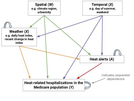
Figure 1: Diagram of our system.

While the potential for harnessing RL for public health applications has been noted previously (Weltz et al., 2022), our case study will show that out-of-the-box RL methods are inadequate to solve the problem of optimizing heat alert issuance for health. To address this gap, we propose conceptually simple yet effective modifications to the RL workflow, generating statistically significant improvements over the observed NWS policy and offering pragmatic domain insights.

Our framework for training and evaluating RL for heat alert issuance under an intervention budget uses a decision-making environment combining Bayesian statistical modeling and sampling of exogenous weather trajectories, followed by a detailed contrastive analysis of the resulting RL policies. The four main steps can be summarized as follows. (1) First, we model hospitalizations as a function of relevant variables for decision-making (e.g. weather and heat alert history), which identifies the health impact of heat alerts prior to the SDM policy optimization. We use a Bayesian hierarchical model which facilitates interpretation and uncertainty quantification in our heterogeneous setting. To account for spatial heterogeneity while allowing information sharing across locations, our model pairs fixed effects for each location with a data-driven prior that is a function of location-specific confounders and effect modifiers. This model is fit using deep learning and variational inference for scalability (Wang et al., 2019). (2) Second, we use the Bayesian model estimates as the reward function in a realistic SDM environment. We leverage the exogenous nature of the weather (relative to our alert interventions) to bypass the need for learning a transition model for the environment, which is required in standard model-based RL (Moerland et al., 2023). Our approach applies broadly for environmental / climate change-related applications and others with exogenous inputs (Sinclair et al., 2022). All together, this constitutes what we call the BROACH (Bayesian Rewards Over Actual Climate History) simulator for SDM. (3) Third, we use the BROACH simulator to train RL models and evaluate this and other policies – all subject to the same alert budget – for comparison. We introduce modifications to the standard RL training paradigm that are needed to obtain policies that outperform the NWS policy, such as restricting the available interventions to extremely hot days, optimizing policies for each location separately, and augmenting the available training episodes with exogenous data from similar locations. (4) Fourth, we perform contrastive explanation (van der Waa et al., 2018; Narayanan et al., 2022) of the RL policies by comparing their attributes within and across locations to those of the NWS and other benchmark policies. Specifically, we use a variety of visualizations as well as Classification and Regression Trees (CART) to illustrate systematic differences between these policies, provide intuition about their underlying dynamics, and identify characteristics of locations where RL offers the greatest public health benefits over the alternative policies.

Throughout the analysis, we use standardized, publicly-available code bases to deploy state-of-the-art algorithms and facilitate others’ use of these tools. To promote future work on this problem and related applications, we plan to publish all our code as well as the BROACH simulator for heat alerts at the time of paper publication.

This work builds off many different strands of literature. Recent approaches to improving the issuance of heat alerts include (i) development of a causal inference technique for stochastic interventions to infer whether increasing the probability of issuing a heat alert would be beneficial (Wu et al., 2023) and (ii) a comparison of methods for identifying optimal thresholds above which heat alerts should always be issued (Masselot et al., 2021). Crucially, neither of these approaches addresses the complications of sequential dependence, i.e. the potential for alert fatigue and running out of resources to deploy precautionary measures. To our knowledge, SDM techniques have yet to be explored in the environmental health setting. More generally, the use of Bayesian modeling in RL is a broad, established topic (Ghavamzadeh et al., 2015; Tec et al., 2023), including use of a Bayesian rewards model to identify the effect of intervention in health-related applications (Liao et al., 2020) as well as use of Bayesian hierarchical models in dynamic treatment regimes (Zajonc, 2012). In spatiotemporal or otherwise heterogeneous environments, previous papers have also used a combination of local modeling and global modeling accounting for spatial or hierarchical structure to create simulated environments for RL (Wu et al., 2021; Li et al., 2018; Agarwal et al., 2021). The use of domain knowledge-based policy restrictions has been observed to speed up RL optimization (Mu et al., 2021) and constrain the cost of actions (Laber et al., 2018). Another important swath of literature surrounds interpretability (intrinsic) and explainability (post-hoc) methods in RL. There are many recent surveys of this topic (Heuillet et al., 2021; Glanois et al., 2022). We note that while CART has been used to try and mimic RL policies (Puiutta and Veith, 2020), our use of it to analyze differences between policies’ performance is more novel.

The rest of the paper will be structured as follows. Section 2 describes the observational data set used in this case study, including our specific health outcome. Section 3 introduces the SDM notation and RL algorithms we use. Section 4 details the development of the BROACH simulator (including the hierarchical Bayesian rewards model and handling of exogenous variables such as weather) as well as our RL analysis (including modifications during training, evaluation methods, and post-hoc contrastive analysis). Section 5 shares our results from the rewards modeling and the RL analysis. Section 6 discusses our study’s contributions and limitations as well as directions for future work.

2 Data

We use a US county-level dataset which has been used in past studies of heat alert effectiveness (Wu et al., 2023; Weinberger et al., 2021). This dataset contains daily observations from the warm months in 2006 through 2016. For this study, we define the warm season / summer to be May through September, and focus only on the 761 (24% of) counties with population greater than 65,000 to avoid numerical instability from small daily hospitalization rates. Primary features in the dataset include population-weighted maximum heat index (henceforth referred to as ”heat index”, which takes into account both temperature and relative humidity), whether a heat alert was issued by the NWS, and hospitalizations from Medicare claims.

To account for people’s likely climate adaptation, our analyses make use of the quantile of heat index (within each county, across all the years) as well as the absolute heat index. Additionally, we compiled county-level estimates of other features to help characterize variability in the health impacts of extreme heat and heat alerts: population density and median household income (U.S. Census Bureau, 2014), regional climate zone classifications (U.S. Energy Information Administration, 2020), broadband (internet) usage data (Microsoft AI for Good Research Lab, 2021), presidential election returns (MIT Election Data and Science Lab, 2018), and PM_2.5 air pollution (Hammer et al., 2020). For the latter: there is strong evidence of adverse synergistic health impacts of air pollution and heat (Anenberg et al., 2020). These spatial characteristics are complemented by temporal variables such as day of summer (days since the first of May) and a weekend indicator.

The Health Outcome

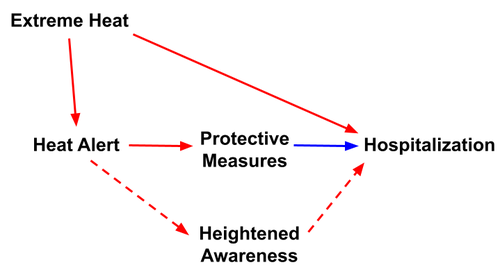
Figure S1: Mediation of the effect of heat alerts on hospitalizations for obviously heat-related symptoms / causes. Dashed lines indicate the effect that we are not interested in identifying.

Cause-specific hospitalizations previously found to be associated with extreme heat in the Medicare population (Bobb et al., 2014) are fluid and electrolyte disorders, renal failure, urinary tract infections, septicemia, heat stroke and other external causes, peripheral vascular disease, and diabetes mellitus with complications. However, Weinberger et al. (2021) observed increased hospitalizations for fluid and electrolyte disorders and heat stroke on heat alert days (while accounting for confounding by extreme heat) and inferred that heat alerts may encourage more seniors to seek or access health care. We recognize this as a mediation problem, as illustrated in Figure S1. One potential effect of seeing a heat alert is that people take actions to reduce their exposure to extreme heat / mitigate the effects of exposure (thereby reducing adverse health outcomes), but another potential effect of seeing a heat alert is to recognize heat-related symptoms that are already occurring, prompting a trip to the hospital. The “mediator” in this case is people’s common sense about what symptoms are heat-related (i.e. dehydration and fainting). This leads to the (potential) protective effect of heat alerts not being identifiable in hospitalization data for causes that are obviously heat-related.

To avoid the mediation issue described above, we create a pooled hospitalizations variable, henceforth referred to as not-obviously-heat-related (NOHR) hospitalizations, that excludes fluid and electrolyte disorders and heat stroke. We use this pooled outcome rather than individual causes throughout the analysis. About 10% of variation in daily county-level Medicare NOHR hospitalization rate is explainable by our feature set. Descriptive statistics of heat index, NWS heat alerts, and NOHR hospitalizations are in Appendix A.

We note that environmental health policy-making frequently focuses on mortality rather than morbidity. However, the association between heat alerts and mortality, conditional on heat exposure, is weak (Weinberger et al., 2018, 2021): less than 3% of variation in daily county-level mortality rate is explainable by our feature set. This extremely low heat alert-mortality signal led us to use hospitalization data to better enable policy optimization.

3 Background: Reinforcement Learning

The general approach of RL is to deploy an algorithmic ”agent” in an environment in which it attempts to maximize a reward by optimizing its actions. Once trained, RL can be used to make decisions in real time, and to update itself if necessary. Here, we lay out the notation and general mechanics of this powerful tool.

3.1 Markov Decision Processes

Most RL methods assume a Markov Decision Process (MDP). An MDP is a formulation of a dynamical decision-making system where the next state conditional on the current state and action is independent of all prior states and actions. Formally, an MDP is a tuple $\langle S,A,R,P,\gamma\rangle$ where $S$ is the state set, $A$ is the set of available actions, $R:S\times A\rightarrow\mathbb{R}$ is the expected reward function, $P:S\times A\times S\rightarrow[0,1]$ is the transition function, and $\gamma$ is the reward discount factor (Sutton and Barto, 2018). The objective is to find a policy $\pi^{*}(a_{t}|s_{t})\rightarrow[0,1]$ that maximizes the finite-horizon value function $J(\pi)=E_{\pi}\big{[}\sum_{t=0}^{H-1}\gamma^{t}R(s_{t},a_{t})\big{]}$, also referred to as the objective. In our analysis, let each summer / warm season ($H=152$ days) in each county be considered an episode. The action $a_{t}$ on each day is either 1 (issue a heat alert) or 0 (do not issue a heat alert). The state vectors $s_{t}$ and $s_{t+1}$ contain the spatial and temporal characteristics of each county-day, such as weather, weekend status, and number of alerts issued prior to the given day. It is assumed that the state space is sufficient to characterize the MDP, allowing any unobserved factors to be treated as noise with respect to the estimated reward and transition functions. The reward $r_{t}$ is sampled from the modeled distribution of NOHR hospitalizations given $(s_{t},a_{t})$, formally defined in section 4.1. Finally, because from a public policy perspective we care about all hospitalizations during a summer equally, we use discount factor $\gamma=1$.

3.2 RL Algorithms

There are a few major families of RL algorithms which have been extensively studied and applied in numerous domains: value learning, policy learning, and actor-critic. An overview of the development of different branches of RL can be found in Shakya et al. (2023). For the heat alerts analysis, we focus on two of the most commonly used algorithms from value learning and policy learning respectively (Arulkumaran et al., 2017): deep Q-learning (DQN) and Trust Region Policy Optimization (TRPO). While detailed descriptions of these two algorithms are beyond the scope of this text (and can be found in Han et al. (2023)), several distinctions are critical for understanding our analysis and discussion.

The ”policy” learned by DQN is to take whichever action the algorithm estimates would have the largest cumulative reward ($Q$) across the rest of the episode, assuming greedy decisions at each step as described recursively by the Bellman equation $Q^{*}(s_{t},a_{t})=r(s_{t},a_{t})+\gamma E_{s_{t+1}}[max_{a_{t+1}}Q^{*}(s_{t+1},a_{t+1})]$. Because these are not necessarily the actions that the algorithm will take later on, DQN is called an off-policy method (Sutton and Barto, 2018). Crucially, in the absence of additional exploration modifications (e.g. Epsilon-Greedy), the DQN policy is deterministic: the fitted model will always make the same decisions given the same inputs. By contrast, TRPO is an on-policy method that directly optimizes a stochastic policy: it uses gradient ascent on the RL objective $J(\pi)$ to find the best parameters for its policy function $\pi_{\theta}(a|s)$, which outputs a probability for each action given the current state. To deploy such a policy, the action is sampled from a Multinomial (or in our case, Bernoulli) with these probabilities.

Imposing Constraints

Traditional RL algorithms such as DQN and TRPO were designed for MDPs with unlimited actions available. However, in the heat alerts setting there is a ”cost” to each action: both individuals and communities likely have diminished will and resources to respond to any single alert as more alerts are issued. Therefore, we take an action budget-constrained RL approach, maximizing $J(\pi)$ such that $\sum_{t=0}^{H-1}a_{t}\leq b$; this budget $b$ will be clarified in section 4.1. Unfortunately, constrained or budgeted MDPs are not as easily solvable as regular MDPs (Carrara et al., 2019). Incorporating cost or safety constraints in RL is an active area of research (Laber et al., 2018; Xu et al., 2022).

Related to but distinct from the need to limit the number of heat alerts is the challenge for RL of exploring and identifying an optimal policy over a relatively long horizon, in our case the 152 days in each warm season. Previous work has shown that imposing domain knowledge-based constraints can help to both guide the learned policy in pragmatic directions and speed up the overall learning process (Mu et al., 2021). Additionally, domain knowledge-based constraints – such as a restriction of heat alerts to extremely hot days – have the benefit of being relatively interpretable.

4 Methods

4.1 Bayesian Rewards Over Actual Climate History (BROACH)

To learn and evaluate new policies for heat alerts, we require an interactive environment that generates both transitions between states and rewards in response to the actions taken at each state, which together characterize the MDP. We create a simulator called Bayesian Rewards Over Actual Climate History (BROACH), which can easily be adapted for other types of weather- or climate-related exposures and interventions. A distinctive aspect of such applications is that the underlying dynamical driver, the weather / climate, is very complex: attempting to model it would be a massive undertaking, and in any case might reduce variability in daily weather that is actually critical for informing interventions such as heat alerts. Thus, BROACH utilizes real observed weather trajectories to generate transitions $P(s_{t+1}|s_{t},a_{t})$. This technique is valid because weather / climate is a completely exogenous component of the MDP: an RL agent’s actions cannot affect it. By contrast, when generating the rewards $r_{t}$, we develop a model that takes into account all aspects of the system: weather, heat alerts, and other social and environmental factors that confound or modify the health effects of interest. We use a Bayesian hierarchical regression to flexibly model NOHR hospitalizations, accounting for spatial heterogeneity and sequential dependence of alerts, while enabling domain-relevant interpretations and uncertainty quantification obtained via modest computation. This model incorporates spatial information via a data-driven prior, which facilitates the optimization and interpretation of RL policies for individual locations – in our case, counties. The utility of single-county RL is highlighted in our post-hoc analysis, described in section 4.2.

Sampling Exogenous Transitions

To formalize the transitions component of BROACH, let $s_{t}=(x_{t},\xi_{t})$ where $\xi_{t}$ are the exogenous variables such as heat index and $x_{t}$ are the endogenous (and deterministically-updating) variables such as past heat alerts. Let $\boldsymbol{a},\boldsymbol{x},\boldsymbol{\xi}$ be the trajectories $(a_{0},...,a_{H-1})$, $(x_{0},...,x_{H-1})$, and $(\xi_{0},...,\xi_{H-1})$ respectively, and let $\{\boldsymbol{\xi}^{(i)}\}_{i=1}^{N}$ denote a sample of $N$ trajectories of $\xi$. Because $\boldsymbol{\xi}$ is exogenous, the objective function $J(\pi)=E_{\pi}\Big{[}\sum_{t=0}^{H-1}R(s_{t},a_{t})\Big{]}$ can be rewritten (proof is in Appendix B) and approximated using Monte Carlo:

$$J(\pi)=E_{\boldsymbol{\xi}}\Big{[}E_{\boldsymbol{a},\boldsymbol{x}}\Big{[}\sum_{t=0}^{H-1}R(x_{t},\xi_{t},a_{t})|\boldsymbol{\xi}\Big{]}\Big{]}\approx\frac{1}{N}\sum_{i=1}^{N}E_{\boldsymbol{a},\boldsymbol{x}}\Big{[}\sum_{t=0}^{H-1}R(x_{t},\xi_{t}^{(i)},a_{t})\Big{]}$$ (1)

One issue with this approach is that there are only 11 exogenous trajectories available per county. To mitigate the potential for overfitting, we propose data augmentation by sampling weather trajectories from other counties in the same regional climate zone (U.S. Energy Information Administration, 2020) during RL training and validation / tuning.

Our decomposition of exogenous vs endogenous components of the state space using Monte Carlo approximations was partially inspired by Efroni et al. (2022), who provide a theoretical analysis and guarantees for sample efficiency with a finite-state exogenous space (which is not the case for weather / climate), as well as by Sinclair et al. (2022), who introduce a method called hindsight learning for situations where a known reward function and an exact solver under a fixed exogenous trajectory are available (neither of which are available for heat alerts).

Modeling the Rewards

We desire a model for the rewards that deals with low signal in the heat alert-health relationship, allows for spatial heterogeneity in the effects of heat and heat alerts, and facilitates both interpretation and uncertainty quantification that will scale to large data. To achieve this, we formulate a Bayesian hierarchical model that pairs fixed effects for each location with a prior that depends on spatially-varying features. Relegating these spatial variables to the prior streamlines single-county RL because those features can be ignored during policy optimization. Let $k\in\mathcal{K}$ and $t\in\mathcal{T}$ denote a county and time (in days), respectively. Let $Y_{k,t}$ be the number of NOHR hospitalizations and $A_{k,t}$ be whether or not a heat alert was issued. Let $S_{k,t}$ be the temporally-varying covariates at location $k$ and $W_{k}$ be the spatially-varying but temporally static covariates, to be used in the prior. The model is given by:

$$Y_{k,t} \sim\text{Poisson}(N_{k,t}*\lambda_{k,t}*(1-A_{k,t}\tau_{k,t})),\>\>\>\>\>\lambda_{k,t}=exp(\beta_{k}^{\top}S_{k,t}),\>\>\>\>\>\tau_{k,t}=sigmoid(\delta_{k}^{\top}V_{k,t})$$

where $N_{k,t}$ is the summer-specific mean of NOHR hospitalizations at location $k$, $\lambda_{k,t}$ is the baseline variation from $N_{k,t}$ (with mean 1), and $V_{k,t}$ is a subset of $S_{k,t}$. $\tau_{k,t}$ is the multiplicative effect of issuing an alert, which is allowed to vary based on the features in $V_{k,t}$. $\tau_{k,t}$ is constrained to be between 0 and 1, such that issuing a heat alert is never harmful (never leads to an increase in the hospitalization rate relative to baseline), with larger values of $\tau$ indicating larger protective effects of alerts. The desire to constrain $\tau$ – helping to mitigate the low-signal issue – as well as to stabilize the estimation of $\lambda$ informed our somewhat unconventional formulation of the Poisson model.

Then, for the RL in county $k$, the rewards are $r_{t}=1-\lambda_{k}(s_{t})*[1-a_{t}*\tau_{k}(v_{t})]$.

Here, $V_{k,t}$ contains (1) that day’s quantile of heat index (QHI); (2) excess heat, which we define as the difference between the QHI and the average of the last three days’ QHI (a time window informed by the literature on heat waves and health (Metzger et al., 2010)); (3) an indicator of whether a heat alert was issued yesterday; (4) the total number of heat alerts over the past two weeks; (5) an indicator of whether it’s a weekend day; and (6) a spline (df=3) on day of summer. $S_{k,t}$ additionally includes the change in QHI above the 25th percentile and that above the 75th percentile, to allow for a piecewise-linear main effect of QHI. The features in $W_{k}$, used in the prior, are log of population density, log of median household income, annual average $PM_{2.5}$ concentration, percent of homes using broadband (Internet), and the fraction of votes for a Democratic president in the last election.

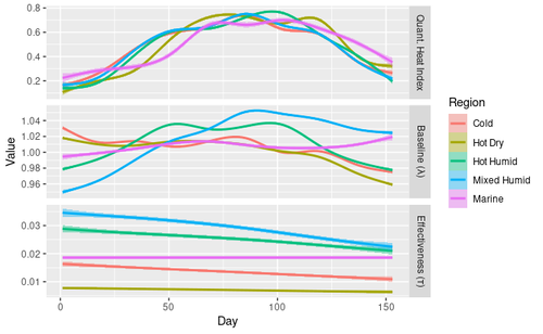
Figure S3: Smoothed trajectories of observed quantile of heat index, modeled baseline NOHR hospitalizations, and modeled alert effectiveness (assuming no past alerts) across days of summer; colored by climate region.

The data-driven priors for $\beta_{k}$ and $\delta_{k}$ are modeled using multilayer perceptrons (MLP), each with one hidden layer of 32 units. To further incorporate domain knowledge, we impose constraints on a few of the coefficients in $\beta$ and $\delta$. Without a constraint, a variable is sampled from a Normal with mean $x\sim MLP(W_{k})$ and standard deviation 1. For a variable constrained to be positive, we use a LogNormal instead of a Normal; for a variable constrained to be negative, we use a Negative LogNormal. For consistency with our assumption that issuing heat alerts is not harmful relative to issuing zero heat alerts, we impose that the $\beta_{k}$ for the past alert variables should be negative, corresponding to less (or no change in) baseline hospitalizations when there are more past alerts. To ensure that the model doesn’t put too much weight on the few less-hot alert days in our empirical dataset (which are not confined to the early days of summer), we also constrain the $\delta_{k}$ for QHI and excess heat to be positive, corresponding to greater (or no change in) heat alert effectiveness when it is hotter. Note that this is conditional on day of summer, so it still allows higher alert effectiveness earlier in the summer (see Figure S3), when heat index may not be as high but heat alerts may come as more of a surprise to people.

To fit this Bayesian model, we use the Python package Pyro (Harpole et al., 2019). Specifically, we use stochastic variational inference with a low-rank Multivariate Normal as the guide (variational distribution) for the posterior, allowing for efficient computation while approximating the true correlation structure of the joint probability distribution.

Putting the Pieces Together

We write code in the standard MDP configuration, called Gym (Towers et al., 2023), to create an environment in which sampled trajectories of real weather and posterior samples of the modeled rewards are passed to the RL for county $k$, allowing the RL agent to issue alerts until its budget $b$ for that warm season is reached. For simplicity, we take $b$ to be the observed number of heat alerts issued by the NWS in each county-summer. While in a fully online setting we wouldn’t know the alert budget ahead of time, this approach allows us to tackle the issue of when to issue heat alerts under a budget, saving the question of how many alerts to issue for future work. For our augmented training dataset, we sample $b$ with its corresponding weather trajectory, so $b$ is lumped into the exogenous $\boldsymbol{\xi}$. Incorporating sampled coefficients $\{r^{(j)}\}_{j=1}^{M}$ from the rewards model posterior, equation (1) becomes:

$$J(\pi)\approx\frac{1}{N}\frac{1}{M}\sum_{i=1}^{N}\sum_{j=1}^{M}E_{\boldsymbol{a},\boldsymbol{x}}\Big{[}\sum_{t=0}^{H-1}r^{(j)}(x_{t},\xi_{t}^{(i)},a_{t})\Big{]}$$ (2)

An algorithmic summary of our sampling procedures is provided in Appendix D.

In addition to the covariates used in the Bayesian rewards model, the RL state space includes the number of remaining alerts allocated for that episode ($b-\sum_{d=0}^{t-1}a_{d}$) as well as a rolling average of the absolute heat index for each county-summer, as was used in the stochastic intervention analysis of heat alerts (Wu et al., 2023).

4.2 RL Analysis

Unsurprisingly, the counties for which NWS issued few heat alerts had unreliable estimates of heat alert effectiveness in our rewards model. Thus, for the RL phase, we chose to only consider counties where at least 75 heat alerts were issued across the 11 years. This left 170 counties. For computational and analytical purposes, we further subset this to 30 counties using the following criteria: for each climate region, select the county with the highest variance in estimated heat alert effectiveness (indicating higher signal identified by the rewards model). To get up to 30, repeat this selection, but first prioritize selecting a county from a US state not already in the set, and if we must repeat a state, do not select a county that is directly adjacent to one already in the set. If there are no more eligible counties in a region, select from a larger region. Characteristics of these 30 counties are summarized in Table S3.

Training

To run the DQN and TRPO algorithms, we use the popular Python package Stable Baselines (Raffin et al., 2021). We ran each of the models for 15 million training iterations (about 100,000 episodes), a sufficient horizon for convergence.

A major challenge for our RL models under the budget is learning to conserve alerts for later in the summer. To encourage this behavior, we restrict the issuance of heat alerts to days above a QHI threshold, optimized separately for each county. To optimize the QHI threshold, we test the sequence of values between 0.5 and 0.9 (an interval selected to ensure overlap with the NWS policy without being too restrictive), by every 0.05, and select the value that yields the best return on our validation set, which is specified in the following section. Names of models including this adaptation have the suffix ”.QHI”.

As a sensitivity analysis, we investigate whether the RL models can learn to anticipate the general trajectory of weather / sub-seasonal variation in the warm season by augmenting the RL state space with information about the future. Specifically, we test whether inclusion of the change in heat index over each of the next 10 days as well as the 50th-100th (by every 10) percentiles of QHI for the remainder of the summer improves RL performance. In real-time deployments of RL models, this kind of future information would not be known but could be sourced from either weather forecasts or climate model predictions. Of course, such forecasts / model predictions are not perfect, but we start with perfect future information as a proof of concept. Names of models including future information have the suffix ”.F”.

Evaluation

In our main analysis, we allow each algorithm to issue the type of policy that it optimizes during training: deterministic for DQN and stochastic for TRPO. As a sensitivity analysis, we evaluate the TRPO policy deterministically, selecting whichever action has a higher probability under the policy function. To evaluate each of the RL policies, we compare them to the observed NWS policy as well as several other counterfactual policies: most simplistically, issuing zero alerts, selecting $b$ days randomly (random), and selecting the $b$ days with the highest QHI that summer (topk). We also implement the general guidelines that NWS recommends in the absence of local criteria for issuing heat alerts (basic.nws): alert if the heat index is $\geq 100^{\circ}$F in northern states and $\geq 105^{\circ}$F in southern states (Hawkins et al., 2017). Lastly, we implement a policy of always issuing alerts on days above an optimized QHI threshold until the budget runs out (aa.qhi).

The main metric we use for policy comparison is the average cumulative reward per episode (”average return”). To estimate this metric fairly, we hold three years of data (2007, 2011, and 2015) out from RL training – referred to as the evaluation years. For the purposes of RL hyperparameter tuning (details in Appendix C) and selection of the optimal QHI threshold for each county, we consider the regionally-augmented weather trajectories and associated budgets from the evaluation years excluding the county of interest to be the validation dataset. The final evaluation results (reported in tables and figures) are obtained by drawing 1,000 sets of coefficients from the rewards model posterior and calculating the return under each policy with weather and budgets only from the county of interest during the evaluation years. These validation/tuning and evaluation procedures are described algorithmically in Appendix D. After calculating the average returns for the 30 counties under each competing policy, we compare each policy’s returns with the associated returns under the observed NWS policy for the same counties and years using a Wilcoxon-Mann-Whitney test.

Post-hoc Contrastive Analysis

To investigate why some counties see smaller (or even no) benefits from the application of the heat alerts RL, we consider both stationary features included upstream in the analysis (e.g. climate region, median household income) as well as characteristics of both the NWS and counterfactual alert policies, namely the distributions of the days of summer on which alerts are issued and the lengths of alert streaks (sequences of repeated alerts). To structure this exploration, we fit CART on both the numeric difference in average return and a binary indicator of whether this difference is positive (i.e. the RL performed better), comparing the best RL model with (a) the NWS policy and (b) the best counterfactual benchmark policy. To prevent CART overfitting to our 30 counties and to facilitate interpretation, we limit the maximum depth of the trees to 2.

5 Results

This section illustrates the viability of the rewards model in our BROACH simulator as well as how the resulting RL policies perform relative to the NWS and other intuitive benchmarks. Our post-hoc analysis identifies scenarios where RL offers the greatest improvement over current heat alerts policy.

5.1 Fitted Rewards Model

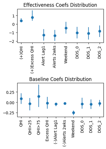
Figure 2: A sample of posterior coefficients from the rewards model (in $\tau$ and $\lambda$ respectively), with IQR and median shown. (+)/(-) indicates a coefficient constrained to be positive/negative. DOS_[0-2] is the spline (df=3) on day of summer.

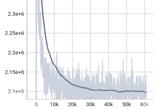
Figure S2: Convergence of the loss of the Bayesian rewards model across training (80 epochs).

The rewards model clearly converged in its loss across epochs (shown in Figure S2) and achieved higher predictive accuracy than standard machine learning algorithms (i.e. random forest, neural network). Predicting the rate of NOHR hospitalizations in the Medicare population in each county, this model has $R^{2}=0.102$, using the calculation $SSR/SST$ for comparability with earlier machine learning models (such as that we used when checking the signal in the mortality data). Predicting the absolute number of NOHR hospitalizations, it has $R^{2}=0.884$ (much higher because the value is mostly driven by county population size). The model also displayed very good coverage when we ran it on synthetic data (1,000 samples from the posterior predictive) using known coefficients: average coverage across parameters for 90% CI was 0.897. Figure 2 shows one posterior sample across the 761 counties on which the model was fit. Note that the spread across counties is larger than the spread within counties, so the IQR bars are no larger for multiple samples. Overall, we see that the coefficients on past alerts in today’s alert effectiveness ($\tau$) are both negative, empirical evidence of alert fatigue. In the baseline hospitalization rate ($\lambda$), we see a strong protective effect by weekend.

5.2 RL Analysis

Policy Evaluations

				NOHR Hosps Saved vs NWS (vs Zero) Per Summer
Policy	Median Diff.	WMW	P-value	Median / 10,000 Medicare	Approximate Total
random	-0.015	177	0.88	-0.013 (1.98)	-64 (9,697)
basic.nws	-0.286	30	1.0	-0.283 (1.45)	-1,388 (7,110)
aa.qhi	0.03	348	0.0025	0.029 (1.99)	143 (9,747)
dqn	-0.123	43	0.99995	-0.102 (1.83)	-502 (8989)
trpo	-0.065	97	0.99742	-0.063 (1.9)	-309 (9321)
dqn.qhi	0.03	370	0.00242	0.029 (1.99)	142 (9746)
trpo.qhi	0.038	338	0.0154	0.038 (2.02)	185 (9897)
*topk	0.022	406	0.0002	0.023 (1.96)	113 (9,603)

Table 1: Comparison between the average return of each counterfactual policy and that of the NWS policy on the evaluation years, summarized across counties (e.g. ”Median Diff.” is the median difference in average return). The last two columns also provide a comparison to the counterfactual with zero heat alerts. WMW is the Wilcoxon-Mann-Whitney statistic (higher is better); its associated p-value is also included. The last policy (marked by *) is oracle. The approximate total number of hospitalizations is based on 49 million Medicare enrollees in 2011 (CMS, 2011).

Table 1 provides the main results from our RL experiments. We first note that several counterfactual policies perform worse than NWS (as indicated by negative median differences in returns): random, basic.nws, and the RL models without the QHI restriction. By contrast, the RL models with the QHI restriction perform significantly better than NWS, as indicated by their significant positive median difference in returns. In absolute terms, a very rough estimate if trpo.qhi were implemented as-is across all counties in the US (using the Medicare population from 2011, the midpoint of our study period) is that we could see a reduction of 185 NOHR hospitalizations per year.

Our sensitivity analysis revealed two important points. The first is that the addition of future information in the RL models’ state space (results in Table S2) had different effects depending on the algorithm. Across both plain and QHI-restricted models, it made trpo a bit better but dqn much worse. The latter may be due to overfitting, given that dqn.qhi.f did fine in the validation / tuning stage but proceeded to issue zero alerts in all but one county in the final evaluation stage. For the trpo models, the benefit observed with use of future information would likely be smaller in practice due to forecast / prediction error – the simulation of which is beyond the scope of this paper. We also note that the behavior (described in the following section) of trpo.qhi and trpo.qhi.f is quite similar. Therefore, we focus on the RL models without future information in the rest of this paper.

The second point determined via sensitivity analysis is that interpreting policies from TRPO models deterministically fails in the heat alerts setting under our rewards model. This is because many of the policy functions’ estimated probabilities for issuing an alert are below 0.5, so always taking the action with the larger probability dramatically reduces the number of alerts issued – in some counties to zero. Note that policies which do not use all the alerts in their budget are penalized under our rewards model, resulting in trpo.qhi no longer outperforming NWS with statistical significance across the 30 counties.

When compared to the policies of always issuing an alert on days above an optimized QHI threshold (aa.qhi) and of issuing alerts on the $b$ hottest days of the summer (topk), which also perform signficantly better than the NWS, the relative performance of RL (subject to a QHI restriction) is less clear. First, we note that the performance and behavior of dqn.qhi is nearly identical to aa.qhi – the former is not even shown in Figures 3 or 4 because it is visually indistinguishable from the latter. Thus, we focus on trpo.qhi as the more complex alternative SDM policy. Among trpo.qhi, aa.qhi, and topk, the ordering of median difference in returns (compared to NWS) is opposite the ordering of these policies’ Wilcoxon-Mann-Whitney statistics. This is because of the longer tails of the trpo.qhi differences, as illustrated in Figure 3. Note that topk is an oracle (not implementable) policy because to use it we would have to know the QHI for the whole warm season in advance. However, aa.qhi is an implementable alternative to trpo.qhi, so we must consider it more seriously.

Contrastive Explanations

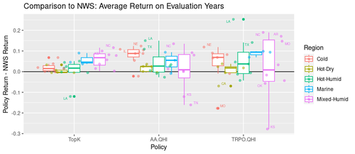
Figure 3: Different policies’ average return relative to NWS across different climate regions, on the evaluation years. Outlier points are labeled with their state abbreviation. Note that topk is an oracle policy.

Figure 3 illustrates the policies’ varying performance relative to NWS across climate regions and counties. A striking visual pattern is the increasing vertical spread from left to right: trpo.qhi exhibits more heterogeneity across counties than aa.qhi, which in turn performs more heterogeneously than topk. Similarly, some climate regions such as Mixed-Humid and Hot-Humid display more heterogeneity across counties than the others, across all the policies. This is partially due to those regions being larger and thus over-represented among our 30 counties (see Table S3), but that does not fully explain the discrepancy.

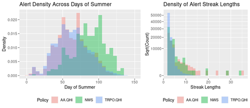
Figure 4: Distributions of heat alert characteristics under different policies, on the evaluation years.

Figure 4 provides some insight into similarities and differences between the NWS, aa.qhi, and trpo.qhi policies. In the histogram on the left, we see that both counterfactual policies tend to issue heat alerts earlier in the summer than NWS. The histogram on the right indicates that the RL tends to issue shorter streaks of alerts, which makes sense given its ability to learn sequential dependence encoded by the rewards model.

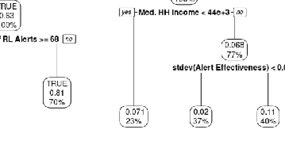
Figure 5: Classification (left) and regression (right) tree diagrams comparing trpo.qhi to NWS. ”TRUE” and positive values, respectively, indicate the RL performing better. The percentage in each node indicates the fraction of counties in that subgroup. In the classification tree, the middle number is the predicted probability. DOS is the day of summer / warm season and Alert Effectiveness is the $\tau$ estimated by our rewards model.

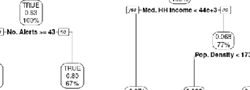
Figure S5: Classification (left) and regression (right) tree diagrams comparing trpo.qhi to NWS, using only non-modeled variables. ”TRUE” and positive values indicate the RL performing better. ”No. Alerts” is the sum of alerts issued by NWS during the evaluation years.

The CART analysis provides further nuance. In Figure 5, the classification tree indicates that the most predictive feature of trpo.qhi performance relative to NWS is the median day of summer on which the RL issued heat alerts. Specifically, improvement is observed in counties for which the RL identified that it is optimal to issue alerts earlier in the summer. Whereas, in counties for which it is optimal to issue alerts later in the summer, there was less room for improvement by the RL because the NWS already tends to issues alerts later in the summer. The regression tree offers complementary intuitions. The second split in the regression tree indicates that the RL performs best when there is greater variation in alert effectiveness across days – in other words, when there is more signal in the heat alert-health relationship that can be leveraged by the RL. This is an expected result. The first split indicates that the RL makes less improvement in counties with lower socioeconomic status. Our intuition is that this is because people in lower-income areas may have less agency to take protective action in response to heat alerts, such as turning on air conditioning and/or working indoors, resulting in less room for optimization by RL. We also note that in the set of 30 counties used in our RL analysis, there is a negative correlation between heat alert budget size and median household income, as well as population density. Thus, CART may be indicating a greater benefit to using RL when the alert budget is smaller, possibly because it is then more critical to discriminate days when heat alerts will be most effective. This interpretation is supported by a sensitivity analysis excluding modeled variables from the CART feature set (Figure S5).

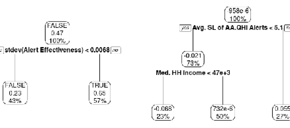
Figure S4: Classification (left) and regression (right) tree diagrams comparing trpo.qhi to aa.qhi. ”TRUE” and positive values indicate the RL performing better. DOS is the day of summer, Alert Effectiveness is the $\tau$ estimated by our rewards model, and SL is the streak length.

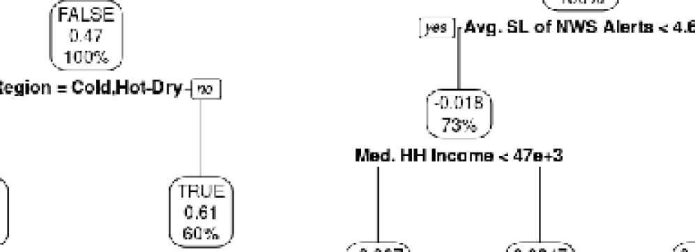
Figure S6: Classification (left) and regression (right) tree diagrams comparing trpo.qhi to aa.qhi, using only non-modeled variables. ”TRUE” and positive values indicate the RL performing better. SL is the streak length.

Next, we compare the performance and characteristics of trpo.qhi and aa.qhi using CART. The results, shown in Figure S4, support our previous conclusions. The classification tree is split on variation in heat alert effectiveness and the regression tree includes a split on median household income, both with the same direction as before. Additionally, the regression tree illustrates the predictive power of the the average length of alert streaks issued by aa.qhi. Specifically, there is more benefit from using RL in counties that tend to experience more prolonged heat waves – prompting aa.qhi to issue more alerts in a row, which is likely to result in alert fatigue. In our sensitivity analysis excluding modeled variables (Figure S6), we see that RL is more likely to yield a larger median difference (compared to NWS) than aa.qhi when the NWS issues longer streaks, echoing the above intuition. Similarly, the classification tree indicates that aa.qhi performs better in the Cold or Hot-Dry climate regions. This makes sense because these regions tend to have lower humidity than the Hot-Humid, Mixed-Humid, and Marine climate regions and thus fewer prolonged heat waves (because humidity tends to slow changes in temperature).

6 Discussion

The primary contributions of this work are (1) formulating and building an SDM pipeline to make progress towards optimizing heat alert issuance for public health, which involved integrating traditional statistical methods with cutting-edge RL techniques, and (2) offering insights into scenarios where RL improves vs fails to improve on the NWS policy or simpler alternatives. This lays the foundation for future work in SDM for environmental health and other climate change-related applications.

One major takeaway from our analysis is that, holding the alert budgets constant, we were able to identify alternative heat alert issuance strategies that outperform the NWS with statistical significance. Large heterogeneity in these effects across counties is consistent with past findings (Wu et al., 2023). Between the RL algorithms, we found that TRPO worked better than DQN, but still required a QHI restriction to be able to learn effectively. Including perfect future weather information in the RL state space benefitted TRPO but not DQN; future work might investigate how noisy such estimates can be before ceasing to improve decision-making.

More ambiguous is whether using a relatively complex method like RL is worthwhile compared with something simpler like aa.qhi, the policy of always issuing an alert above an optimized QHI threshold. While dqn.qhi generated policies indistinguishable from aa.qhi, the relative performance of trpo.qhi differs the county / region. In regions that experience more prolonged heat waves (associated with higher humidity), there is more to be gained from using a model which acknowledges the potential for alert fatigue and can discriminate when it is most beneficial to issue alerts within a heat wave. Unsurprisingly, RL is also more likely to outperform other policies in counties with greater heat alert-health signal, especially earlier in the summer. Regardless of the underlying mechanisms, future work might investigate the application of methods which ensure a new policy is never worse than the existing policy, such as safe policy learning or model predictive control. Alternatively, we could develop a predictive model to select counties that are likely to benefit from RL, using similar intuitions to those in our CART analysis.

Beyond statistical significance in the differences in performance of these policies is the practical significance. Do we estimate substantive health benefits from implementing these improved heat alerts policies? The answer is somewhat subjective, and is discussed in more detail in Appendix E. In general, key points to keep in mind are that (a) heat alerts by themselves are a very cost-effective intervention, so even small reductions in health harms are promising, (b) both the size of the population aged 65+ and exposure to extreme heat events are projected to continue increasing, and (c) the numbers reported in this study should not be interpreted as the overall benefit to public health from improving heat alerts issuance strategies. The health data used in our study only reflect inpatient hospitalizations from NOHR causes billed to Medicare Part A (hospital fee-for-service). Ideally, an optimal heat alerts system would account for different kinds of health impacts experienced by different demographic groups. Future work could explore application of multi-objective RL to consider multiple kinds of health data or even proxies such as missed days of school and mobility data from smartphones / watches.

A general limitation of our analysis is that our results depend on the specification of our rewards model. This is highlighted by the way our simulator penalizes RL models that do not issue all the alerts in their budget, due to constraining the overall effect of heat alerts to not be harmful in the rewards model. We note that there are RL methods which do not require a simulator, instead relying only on past observed data (trajectories). These ”offline” (batch) RL methods are increasing in popularity. However, they too face several major challenges. First, there is a tension between trying to improve on the observed policy and controlling distribution shift (Levine et al., 2020), which can be thought of as the issue of lack of overlap, extrapolation, or lack of generalization in traditional statistical modeling. In our heat alerts application, for instance, we see that the NWS often issues alerts in streaks, making it harder for RL to learn and optimize the impact of each individual alert. Second, assessing the performance of offline RL models using off-policy evaluation (OPE) methods can be difficult. Aspects of the heat alert setting which have been shown to challenge OPE methods include its long episodes, large potential for distribution shift (especially in the absence of a modification such as restricting alerts to very hot days), and high degree of auto-correlation in the reward (Uehara et al., 2022).

Related to constraining the effect of alerts to be non-harmful is our simplification of assuming the heat alerts budget is fixed. Under climate change, the number of extreme heat events is likely to increase. How best to update an alert budget to address a changing system, while simultaneously managing alert fatigue, appears to be an open question. Future work could explore modeling alert fatigue as part of the RL environment, for instance incorporating evidence and/or methods from behavioral science. Similarly, RL algorithms that are intentionally robust to distribution shift (i.e. under climate change) merit investigation in an environmental health setting. Another methodological limitation is that we do not quantify uncertainty spanning the entire analytic pipeline. The Bayesian nature of our rewards model would facilitate this, but it is less straightforward to account for the additional uncertainty from the sampling of weather trajectories, given that we are already using the regionally-augmented set of trajectories for training and validation.

From the domain perspective, development of a stochastic policy (such as that generated by TRPO) may or may not be appealing. On the one hand, it is less immediately satisfying that some aspect of heat alerts issuance would be left to chance. On the other hand, in the context of human-in-the-loop decision making – which would likely be the case for public organizations such as NWS (Stuart et al., 2022) – an algorithm reporting probabilities is more informative than reporting only a binary action. And in any case, if in the future a heat alerts RL model was running continuously online, it would likely need to utilize exploration (incorporating some randomness into its actions) to update itself over time.

Lastly, it is important to acknowledge that issuing heat alerts is only a first step towards reducing the public health impacts of extreme heat: there is much more work to be done analyzing and expanding local actions in response to heat alerts (Errett et al., 2023). If such on-the-ground interventions are able to increase the effectiveness of heat alerts, then this is likely to increase the ability of SDM methods such as RL to identify these effects and help us continue improving our strategies in future.

Conflicts of Interest: The authors have no conflicts of interest to declare.

Author Contributions: To be shared after blind review.

Acknowledgements: To be shared after blind review.

Appendix A Descriptive Statistics of Heat, Alerts, and Hospitalizations

Variable	Min.	Q1	Median	Mean	Q3	Max.
*NOHR hosps per 1,000	5.4 (3.1)	12.5 (12.7)	14.8 (15.2)	15 (15.3)	17.3 (17.8)	25.7 (34.5)
No. of NWS alerts	0 (0)	4 (0)	8 (3)	9.6 (4.8)	13 (7)	43 (57)
DMHI on alert days (°F)	70.5 (68.3)	100.3 (99.7)	103.5 (103.2)	102.5 (102.6)	106.2 (105.9)	121.1 (144)
Q-DMHI on alert days	18.9 (15.6)	91.6 (92.6)	95.8 (96.9)	93.4 (94.2)	98.2 (98.9)	100 (100)
No. of 90th pct. HI days	0 (0)	9 (8)	14 (14)	15.4 (15.4)	21 (21)	46 (61)
DOS of NWS alerts	16 (2)	68 (69)	84 (84)	83.4 (83.5)	99 (99)	142 (150)
DOS of 90th pct. HI days	15 (1)	72 (69)	88 (85)	86.9 (85.2)	102 (102)	145 (153)

Table S1: Summary statistics for our 30 counties of interest (and all the counties) of Medicare NOHR hospitalizations, NWS heat alerts, heat index, and day of summer for several features of interest. DMHI = daily maximum heat index, Q-DMHI = county quantile of DMHI, DOS = day of summer (out of 153). Variables given per county-summer are marked with *.

Table S1 provides descriptive statistics of the heat alerts dataset, both for the 30 counties in our RL analysis (see section 4.2) and all the counties with population $\geq$ 65,000 (used to fit the rewards model). The two sets of statistics are similar aside from the number of heat alerts issued because the counties in the RL analysis were selected specifically for having issued higher numbers of alerts. Other observations are the long tail of the number of NWS alerts per county-summer, that some heat alerts were issued on days that were not very hot in an absolute or relative (quantile) sense, that there were some county-summers with few ”hot” days (90th percentile by county) and others with many, and that the distribution of day-of-summer for NWS heat alerts and 90th percentile QHI by county are quite similar. A few other relevant statistics not shown in the table are that (across all the counties) there were a total of 40,387 heat alerts issued between 2006 and 2016, that 17.2% of NWS heat alerts were issued on days with heat index values that were not in their county’s top 90th percentile, and that 74.0% of days in the top 90th QHI by county did not have NWS heat alerts.

Appendix B Proof Illustrating the Expectation Over the Exogenous Part of the Transition Function

Echoing the notation in section 4.1, let $s_{t}=(x_{t},\xi_{t})$ where $\xi_{t}$ are the exogenous variables such as heat index and $x_{t}$ are the endogenous (and deterministically-updating) variables such as past heat alerts. For simplicity, assume there are no past alerts at $t=0$, so $x_{0}$ is always the same. Let $\boldsymbol{\tau}$ be a trajectory $(s_{0},a_{0},...,s_{H},a_{H})$, let $\boldsymbol{a},\boldsymbol{x},\boldsymbol{\xi}$ be the trajectories $(a_{0},...,a_{H-1})$, $(x_{0},...,x_{H-1})$, and $(\xi_{0},...,\xi_{H-1})$ respectively, and let $\omega(\boldsymbol{a},\boldsymbol{x}|\boldsymbol{\xi})=\prod_{t=0}^{H-1}\pi(a_{t}|x_{t},\xi_{t})P(x_{t+1}|x_{t},\xi_{t},a_{t})$. Also recall that we are using $\gamma=1$. For BROACH, the objective function $J(\pi)$ can be rewritten as:

$$J(\pi) =E_{\pi}\Big{[}\sum_{t=0}^{H-1}R(s_{t},a_{t})\Big{]}$$

$$=\int p_{\pi}(\boldsymbol{\tau})\sum_{t=0}^{H-1}R(s_{t},a_{t})d\boldsymbol{\tau}$$

$$=\int\Big{[}p(s_{0})\prod_{t=0}^{H-1}\pi(a_{t}|s_{t})P(s_{t+1}|s_{t},a_{t})\Big{]}\sum_{t=0}^{H-1}R(s_{t},a_{t})d\boldsymbol{\tau}$$

$$=\int\Big{[}p(\xi_{0})\prod_{t=0}^{H-1}\pi(a_{t}|x_{t},\xi_{t})P(x_{t+1}|x_{t},\xi_{t},a_{t})P(\xi_{t+1}|\xi_{t})\Big{]}\sum_{t=0}^{H-1}R(x_{t},\xi_{t},a_{t})d\boldsymbol{\tau}$$

$$=\int p(\boldsymbol{\xi})\int\omega(\boldsymbol{a},\boldsymbol{x}|\boldsymbol{\xi})\sum_{t=0}^{H-1}R(x_{t},\xi_{t},a_{t})d(\boldsymbol{a},\boldsymbol{x})d\boldsymbol{\xi}$$

$$=E_{\boldsymbol{\xi}}\Big{[}E_{\boldsymbol{a},\boldsymbol{x}}\Big{[}\sum_{t=0}^{H-1}R(x_{t},\xi_{t},a_{t})|\boldsymbol{\xi}\Big{]}\Big{]}$$

Appendix C RL Hyperparameter Tuning

RL algorithms are known to be sensitive to their hyperparameters, especially in empirical settings (Eimer et al., 2022). To address this concern, we tuned hyperparameters per county, using the average return metric. First, we did a broad sweep on one county from each of the five climate regions using trpo.qhi, experimenting with values of learning rate $\in\{0.01,0.001,0.0001\}$, discount factor $\in\{1.0,0.999,0.99\}$, neural network architecture (number of hidden layers $\in\{1,2,3\}$ and number of hidden units $\in\{16,32,64\}$), and size of the replay buffer $\in\{1024,2048,4096\}$; paired with possible QHI thresholds $\in\{0.55,0.7,0.85\}$ and both including and not including future information. After determining that learning rate=0.001 and discount factor=1.0 performed the best across the board, we tuned the remaining parameters for each county and each RL model (all combinations of trpo and dqn with and without QHI restrictions and future information). To make the computation time more reasonable, we did a grid search on two values each for the number of hidden layers (2 or 3), number of hidden units (16 or 32), and size of the replay buffer (1,500 or 3,000).

Appendix D Summary of the Workflow Using BROACH

This section is meant to illustrate a toy example of our workflow. Imagine seven counties located in two climate regions, as shown in the figure below. Let the training years TY = $\{2006,2008,2009,2010,2012,2013,2014,2016\}$ and evaluation years EY = $\{2007,2011,2015\}$.

First, train the rewards model on counties 1-7 and years TY $\cup$ EY to obtain posterior distributions for $r_{1}(s,a),\>...,r_{7}(s,a)$. Then, for each county, follow the steps below. Consider county 1 for illustration.

1:if Training RL (with a QHI restriction) then

2:     for h in $\{0.5,0.55,\>...,\>0.9\}$ do

3:         for i in 1 to $N_{T}$ episodes do

4:              Sample $r_{1,i}(s,a)$ from the posterior for $r_{1}(s,a)$

5:              Sample $\xi_{i}\sim TY\times\{\xi_{1},\xi_{2},\xi_{3},\xi_{4}\}$

6:              Update $\pi_{1,h}(a|s)$ s.t. a = 0 if QHI $<$ h, using $r_{1,i}$ and $\xi_{i}$

7:         end for

8:         Select $\pi^{*}_{1,h}$ (across i) with the largest average return using $\xi_{i}\sim EY\times\{\xi_{2},\xi_{3},\xi_{4}\}$

9:     end for

10:else if Tuning RL or aa.qhi then

11:     for h in $\{0.5,0.55,\>...,\>0.9\}$ do

12:         for i in 1 to $N_{E}$ episodes do

13:              Sample $r_{1,i}(s,a)$ from the posterior for $r_{1}(s,a)$

14:              Sample $\xi_{i}\sim EY\times\{\xi_{2},\xi_{3},\xi_{4}\}$

15:              Calculate cumulative reward using $\pi^{*}_{1,h}$ (or aa.qhi with h), $r_{1,i}$ and $\xi_{i}$

16:         end for

17:     end for

18:     Select h^∗ with the largest return

19:else if Final evaluation for any policy (but using notation for optimized RL) then

20:     for i in 1 to $N_{E}$ episodes do

21:         Sample $r_{1,i}(s,a)$ from the posterior for $r_{1}(s,a)$

22:         Sample $\xi_{i}\sim EY\times\{\xi_{1}\}$

23:         Calculate cumulative reward using $\pi^{*}_{1,h^{*}}$, $r_{1,i}$ and $\xi_{i}$

24:     end for

25:end if

Appendix E Discussion of Absolute Public Health Benefits

For general context: the median rate of NOHR hospitalizations per 10,000 Medicare enrollees per summer during our study period was 148 (Table S1), and we estimated that deploying our best RL model relative to issuing no heat alerts would save 2 of these 148, or 1.4%, in the 30 counties in our RL analysis. Noting that the overall relative risk of a Medicare enrollee experiencing one of the NOHR hospitalization types on a heat wave day is about 1.10 (Bobb et al., 2014), this is substantial evidence in support of continuing to issue heat alerts to protect public health.

Compared to the observed NWS policy, trpo.qhi applied to the 30 counties in our analysis would save approximately 0.038 NOHR hospitalizations per 10,000 Medicare enrollees per summer, a reduction of only 0.03%. Multiplying this by 49 million, the size of the Medicare population in 2011 (the midpoint of our study period), yields about 185 NOHR hospitalizations saved per summer. However, this modest value should be further contextualized by several points.

Firstly, if we take into account the large heterogeneity in the benefit of RL across counties with numbers from the CART diagram (Figure 5), assuming that we figure out how to implement a safe policy such that counties which would not benefit are unaffected, this number increases to 252 ((49m/10k)*(0.4*0.11 + 0.37*0.02)) NOHR hospitalizations saved per summer. This is a very rough approximation given that it assumes the proportion of counties in which RL alert policies were found to improve health outcomes in our sample is generalizable to the rest of the US. It is plausible that our sample of 30 counties is unrepresentative of the US as they tend to have higher variability in alert effectiveness (increasing potential improvements from RL) and also higher alert budgets (decreasing potential improvements from RL).

Secondly, these metrics reflect the climate and Medicare population between 2006 and 2016. We confidently anticipate that both the frequency of extreme heat events under climate change and the size of the Medicare population will continue increasing (Dahl et al., 2019). For instance, while there were 49 million Medicare enrollees in 2011, by 2023 this number has increased to over 65 million, and by 2050 it is projected to be over 85 million (The Boards of Trustees of the Federal Hospital Insurance and Federal Supplementary Medical Insurance Trust Funds, 2023).

Appendix F Supplemental Figures and Tables

				NOHR Hosps Saved vs NWS (vs Zero) Per Summer
Policy	Median Diff.	WMW	P-value	Median / 10,000 Medicare	Approximate Total
dqn	-0.123	43	0.99995	-0.102 (1.83)	-502 (8989)
trpo	-0.065	97	0.99742	-0.063 (1.9)	-309 (9321)
dqn.f	-0.417	40	0.99996	-0.401 (0.49)	-1966 (2408)
trpo.f	-0.062	103	0.99625	-0.061 (1.9)	-297 (9322)
dqn.qhi	0.03	370	0.00242	0.029 (1.99)	142 (9746)
trpo.qhi	0.038	338	0.0154	0.038 (2.02)	185 (9897)
dqn.qhi.f	-1.895	1	1	-1.901 (0)	-9317 (0)
trpo.qhi.f	0.046	345	0.01062	0.048 (2.02)	236 (9886)

Table S2: Extension of Table 1 in the main analysis, illustrating the effect of including future information in the RL state space.

County Fips (State name abbreviation)	Region	No. Alerts (Eval Years)	Population Density (/mi2)	Median HH Income (USD)	Democratic Voters (%)	Broadband Usage (%)	Average PM2.5 ($\mu g/m^{3}$)
5045 (AR)	MxHd	61	179.00	50314.00	34.00	37.50	9.08
20161 (KS)	MxHd	47	120.00	43962.00	43.50	52.20	6.35
21059 (KY)	MxHd	24	212.00	46555.00	38.70	53.30	10.22
29019 (MO)	MxHd	50	242.00	48627.00	51.60	46.60	7.85
37085 (NC)	MxHd	31	200.00	44625.00	39.30	46.70	9.65
40017 (OK)	MxHd	63	133.00	63629.00	22.80	70.10	7.53
47113 (TN)	MxHd	58	176.00	41617.00	44.30	79.40	9.29
42017 (PA)	MxHd	25	1036.00	76555.00	51.00	85.10	9.14
41053 (OR)	Mrn	31	102.00	52808.00	45.60	79.20	3.24
41067 (OR)	Mrn	31	745.00	64180.00	57.70	82.70	4.28
53015 (WA)	Mrn	23	90.00	47596.00	49.40	53.60	3.59
13031 (GA)	HtHd	43	106.00	35840.00	38.90	57.50	9.01
22109 (LA)	HtHd	34	91.00	49960.00	27.90	55.50	8.26
28049 (MS)	HtHd	57	283.00	37626.00	69.90	36.50	8.50
45015 (SC)	HtHd	48	168.00	52427.00	41.20	66.20	8.72
48157 (TX)	HtHd	42	707.00	85297.00	47.80	83.70	8.64
48367 (TX)	HtHd	41	131.00	64515.00	18.30	52.20	7.84
22063 (LA)	HtHd	42	201.00	56811.00	13.70	47.60	8.87
4015 (AZ)	HtDr	29	15.00	39200.00	28.70	63.60	4.59
6025 (CA)	HtDr	40	42.00	41807.00	64.00	64.40	7.22
32003 (NV)	HtDr	29	251.00	52873.00	55.90	78.10	5.21
4013 (AZ)	HtDr	72	423.00	53596.00	44.00	77.40	6.38
6071 (CA)	HtDr	29	103.00	54090.00	51.60	77.10	6.38
17115 (IL)	Cold	22	190.00	46559.00	45.70	63.60	8.87
17167 (IL)	Cold	25	228.00	55449.00	46.00	66.50	8.75
19153 (IA)	Cold	24	764.00	59018.00	54.90	57.90	8.25
19155 (IA)	Cold	27	98.00	51304.00	44.30	42.00	7.89
34021 (NJ)	Cold	29	1639.00	73480.00	67.30	81.60	9.31
29021 (MO)	Cold	44	219.00	44363.00	43.70	48.80	7.97
31153 (NE)	Cold	27	681.00	69965.00	37.60	72.60	7.92

Table S3: Descriptive statistics of the 30 counties used in policy optimization. Climate region abbreviations = {MxHD: Mixed-Humid, Mrn: Marine, HtHd: Hot-Humid, HtDr: Hot-Dry, Cold: Cold}. HH = household. PM_2.5 is an annual average.

References

- Agarwal et al. (2021) Agarwal, A., Alomar, A., Alumootil, V., Shah, D., Shen, D., Xu, Z., and Yang, C. “PerSim: Data-Efficient Offline Reinforcement Learning with Heterogeneous Agents via Personalized Simulators.” In Advances in Neural Information Processing Systems, volume 34, 18564–18576. Curran Associates, Inc. (2021).
- Anderson and Bell (2011) Anderson, G. B. and Bell, M. L. “Heat Waves in the United States: Mortality Risk during Heat Waves and Effect Modification by Heat Wave Characteristics in 43 U.S. Communities.” Environmental Health Perspectives, 119(2):210–218 (2011).
- Anenberg et al. (2020) Anenberg, S. C., Haines, S., Wang, E., Nassikas, N., and Kinney, P. L. “Synergistic health effects of air pollution, temperature, and pollen exposure: a systematic review of epidemiological evidence.” Environmental Health, 19:130 (2020).
- Arulkumaran et al. (2017) Arulkumaran, K., Deisenroth, M. P., Brundage, M., and Bharath, A. A. “Deep Reinforcement Learning: A Brief Survey.” IEEE Signal Processing Magazine, 34(6):26–38 (2017). Conference Name: IEEE Signal Processing Magazine.
- Bobb et al. (2014) Bobb, J. F., Obermeyer, Z., Wang, Y., and Dominici, F. “Cause-Specific Risk of Hospital Admission Related to Extreme Heat in Older Adults.” JAMA, 312(24):2659–2667 (2014).
- Carrara et al. (2019) Carrara, N., Leurent, E., Laroche, R., Urvoy, T., Maillard, O.-A., and Pietquin, O. “Budgeted reinforcement learning in continuous state space.” Advances in Neural Information Processing Systems, 32 (2019).
- CMS (2011) CMS. “2011 CMS Statistics.” Technical report, U.S. Department of Health and Human Services (2011).
- Cutler et al. (2018) Cutler, M. J., Marlon, J. R., Howe, P. D., and Leiserowitz, A. “The Influence of Political Ideology and Socioeconomic Vulnerability on Perceived Health Risks of Heat Waves in the Context of Climate Change.” Weather, Climate, and Society, 10(4):731–746 (2018).
- Dahl et al. (2019) Dahl, K., Licker, R., Abatzoglou, J. T., and Declet-Barreto, J. “Increased frequency of and population exposure to extreme heat index days in the United States during the 21st century.” Environmental Research Communications, 1(7):075002 (2019).
- Ebi et al. (2021) Ebi, K. L., Capon, A., Berry, P., Broderick, C., de Dear, R., Havenith, G., Honda, Y., Kovats, R. S., Ma, W., Malik, A., Morris, N. B., Nybo, L., Seneviratne, S. I., Vanos, J., and Jay, O. “Hot weather and heat extremes: health risks.” The Lancet, 398(10301):698–708 (2021).
- Ebi et al. (2004) Ebi, K. L., Teisberg, T. J., Kalkstein, L. S., Robinson, L., and Weiher, R. F. “Heat Watch/Warning Systems Save Lives: Estimated Costs and Benefits for Philadelphia 1995–98.” Bulletin of the American Meteorological Society, 85(8):1067–1074 (2004).
- Efroni et al. (2022) Efroni, Y., Foster, D. J., Misra, D., Krishnamurthy, A., and Langford, J. “Sample-efficient reinforcement learning in the presence of exogenous information.” In Conference on Learning Theory, 5062–5127 (2022).
- Eimer et al. (2022) Eimer, T., Benjamins, C., and Lindauer, M. “Hyperparameters in Contextual RL are Highly Situational.” (2022). ArXiv:2212.10876 [cs].
- Errett et al. (2023) Errett, N. A., Hartwell, C., Randazza, J. M., Nori-Sarma, A., Weinberger, K. R., Spangler, K. R., Sun, Y., Adams, Q. H., Wellenius, G. A., and Hess, J. J. “Survey of extreme heat public health preparedness plans and response activities in the most populous jurisdictions in the United States.” BMC public health, 23(1):811 (2023).
- Frank et al. (2008) Frank, J., Mannor, S., and Precup, D. “Reinforcement learning in the presence of rare events.” In Proceedings of the 25th international conference on Machine learning, 336–343 (2008).
- Ghavamzadeh et al. (2015) Ghavamzadeh, M., Mannor, S., Pineau, J., and Tamar, A. “Bayesian Reinforcement Learning: A Survey.” Foundations and Trends® in Machine Learning, 8(5-6):359–483 (2015). ArXiv:1609.04436 [cs, stat].
- Glanois et al. (2022) Glanois, C., Weng, P., Zimmer, M., Li, D., Yang, T., Hao, J., and Liu, W. “A Survey on Interpretable Reinforcement Learning.” (2022). ArXiv:2112.13112 [cs].
- Hammer et al. (2020) Hammer, M. S., van Donkelaar, A., Li, C., Lyapustin, A., Sayer, A. M., Hsu, N. C., Levy, R. C., Garay, M. J., Kalashnikova, O. V., Kahn, R. A., Brauer, M., Apte, J. S., Henze, D. K., Zhang, L., Zhang, Q., Ford, B., Pierce, J. R., and Martin, R. V. “Global Estimates and Long-Term Trends of Fine Particulate Matter Concentrations (1998–2018).” Environmental Science & Technology, 54(13):7879–7890 (2020). Publisher: American Chemical Society.
- Han et al. (2023) Han, D., Mulyana, B., Stankovic, V., and Cheng, S. “A Survey on Deep Reinforcement Learning Algorithms for Robotic Manipulation.” Sensors (Basel, Switzerland), 23(7):3762 (2023).
- Harpole et al. (2019) Harpole, A., Zingale, M., Hawke, I., and Chegini, T. “pyro: a framework for hydrodynamics explorations and prototyping.” Journal of Open Source Software, 4(34):1265 (2019).
- Hawkins et al. (2017) Hawkins, M. D., Brown, V., and Ferrell, J. “Assessment of NOAA National Weather Service Methods to Warn for Extreme Heat Events.” Weather, Climate, and Society, 9(1):5–13 (2017).
- Heo et al. (2019) Heo, S., Bell, M. L., and Lee, J.-T. “Comparison of health risks by heat wave definition: Applicability of wet-bulb globe temperature for heat wave criteria.” Environmental Research, 168:158–170 (2019).
- Heuillet et al. (2021) Heuillet, A., Couthouis, F., and Díaz-Rodríguez, N. “Explainability in deep reinforcement learning.” Knowledge-Based Systems, 214:106685 (2021).
- Hondula et al. (2022) Hondula, D. M., Meltzer, S., Balling, R. C., and Iñiguez, P. “Spatial Analysis of United States National Weather Service Excessive Heat Warnings and Heat Advisories.” Bulletin of the American Meteorological Society, 103(9):E2017–E2031 (2022). Publisher: American Meteorological Society Section: Bulletin of the American Meteorological Society.
- Laber et al. (2018) Laber, E. B., Wu, F., Munera, C., Lipkovich, I., Colucci, S., and Ripa, S. “Identifying optimal dosage regimes under safety constraints: An application to long term opioid treatment of chronic pain.” Statistics in Medicine, 37(9):1407–1418 (2018). _eprint: https://onlinelibrary.wiley.com/doi/pdf/10.1002/sim.7566.
- Levine et al. (2020) Levine, S., Kumar, A., Tucker, G., and Fu, J. “Offline Reinforcement Learning: Tutorial, Review, and Perspectives on Open Problems.” arXiv:2005.01643 [cs, stat] (2020). ArXiv: 2005.01643.
- Li et al. (2018) Li, Y., Zheng, Y., and Yang, Q. “Dynamic Bike Reposition: A Spatio-Temporal Reinforcement Learning Approach.” In Proceedings of the 24th ACM SIGKDD International Conference on Knowledge Discovery & Data Mining, 1724–1733. London United Kingdom: ACM (2018).
- Liao et al. (2020) Liao, P., Greenewald, K., Klasnja, P., and Murphy, S. “Personalized HeartSteps: A Reinforcement Learning Algorithm for Optimizing Physical Activity.” Proceedings of the ACM on Interactive, Mobile, Wearable and Ubiquitous Technologies, 4(1):18:1–18:22 (2020).
- Masselot et al. (2021) Masselot, P., Chebana, F., Campagna, C., Lavigne, E., Ouarda, T. B., and Gosselin, P. “Machine Learning Approaches to Identify Thresholds in a Heat-Health Warning System Context.” Journal of the Royal Statistical Society Series A: Statistics in Society, 184(4):1326–1346 (2021).
- Metzger et al. (2010) Metzger, K. B., Ito, K., and Matte, T. D. “Summer Heat and Mortality in New York City: How Hot Is Too Hot?” Environmental Health Perspectives, 118(1):80–86 (2010).
- Microsoft AI for Good Research Lab (2021) Microsoft AI for Good Research Lab. “U.S. Broadband Usage Percentages Dataset.” (2021).
- MIT Election Data and Science Lab (2018) MIT Election Data and Science Lab. “County Presidential Election Returns 2000-2020.” (2018).
- Moerland et al. (2023) Moerland, T. M., Broekens, J., Plaat, A., Jonker, C. M., et al. “Model-based reinforcement learning: A survey.” Foundations and Trends® in Machine Learning, 16(1):1–118 (2023).
- Mu et al. (2021) Mu, T., Theocharous, G., Arbour, D., and Brunskill, E. “Constraint Sampling Reinforcement Learning: Incorporating Expertise For Faster Learning.” (2021). ArXiv:2112.15221 [cs].
- Nahum-Shani et al. (2017) Nahum-Shani, I., Smith, S. N., Spring, B. J., Collins, L. M., Witkiewitz, K., Tewari, A., and Murphy, S. A. “Just-in-Time Adaptive Interventions (JITAIs) in Mobile Health: Key Components and Design Principles for Ongoing Health Behavior Support.” Annals of Behavioral Medicine: A Publication of the Society of Behavioral Medicine, 52(6):446–462 (2017).
- Narayanan et al. (2022) Narayanan, S., Lage, I., and Doshi-Velez, F. “(When) Are Contrastive Explanations of Reinforcement Learning Helpful?” (2022). ArXiv:2211.07719 [cs].
- Ng et al. (2014) Ng, C. F. S., Ueda, K., Takeuchi, A., Nitta, H., Konishi, S., Bagrowicz, R., Watanabe, C., and Takami, A. “Sociogeographic Variation in the Effects of Heat and Cold on Daily Mortality in Japan.” Journal of Epidemiology, 24(1):15–24 (2014).
- Padakandla (2021) Padakandla, S. “A survey of reinforcement learning algorithms for dynamically varying environments.” ACM Computing Surveys (CSUR), 54(6):1–25 (2021).
- Puiutta and Veith (2020) Puiutta, E. and Veith, E. M. “Explainable Reinforcement Learning: A Survey.” (2020). ArXiv:2005.06247 [cs, stat].
- Raffin et al. (2021) Raffin, A., Hill, A., Gleave, A., Kanervisto, A., Ernestus, M., and Dormann, N. “Stable-Baselines3: Reliable Reinforcement Learning Implementations.” Journal of Machine Learning Research, 22(268):1–8 (2021).
- Romoff et al. (2018) Romoff, J., Henderson, P., Piche, A., Francois-Lavet, V., and Pineau, J. “Reward Estimation for Variance Reduction in Deep Reinforcement Learning.” In Conference on Robot Learning, 674–699. PMLR (2018).
- Shakya et al. (2023) Shakya, A. K., Pillai, G., and Chakrabarty, S. “Reinforcement learning algorithms: A brief survey.” Expert Systems with Applications, 231:120495 (2023).
- Sinclair et al. (2022) Sinclair, S. R., Frujeri, F., Cheng, C.-A., and Swaminathan, A. “Hindsight Learning for MDPs with Exogenous Inputs.” (2022). ArXiv:2207.06272 [cs, stat].
- Stuart et al. (2022) Stuart, N. A., Hartfield, G., Schultz, D. M., Wilson, K., West, G., Hoffman, R., Lackmann, G., Brooks, H., Roebber, P., Bals-Elsholz, T., Obermeier, H., Judt, F., Market, P., Nietfeld, D., Telfeyan, B., DePodwin, D., Fries, J., Abrams, E., and Shields, J. “The Evolving Role of Humans in Weather Prediction and Communication.” Bulletin of the American Meteorological Society, 103(8):E1720–E1746 (2022). Publisher: American Meteorological Society Section: Bulletin of the American Meteorological Society.
- Sutton and Barto (2018) Sutton, R. S. and Barto, A. G. Reinforcement Learning: An Introduction. The MIT Press, second edition (2018).
- Tec et al. (2023) Tec, M., Duan, Y., and Müller, P. “A Comparative Tutorial of Bayesian Sequential Design and Reinforcement Learning.” The American Statistician, 77(2):223–233 (2023).
- The Boards of Trustees of the Federal Hospital Insurance and Federal Supplementary Medical Insurance Trust Funds (2023) The Boards of Trustees of the Federal Hospital Insurance and Federal Supplementary Medical Insurance Trust Funds. “2023 Annual Report.” Technical report, Centers for Medicare & Medicaid Services (2023).
- Towers et al. (2023) Towers, M., Terry, J. K., Kwiatkowski, A., Balis, J. U., Cola, G. d., Deleu, T., Goulão, M., Kallinteris, A., KG, A., Krimmel, M., Perez-Vicente, R., Pierré, A., Schulhoff, S., Tai, J. J., Shen, A. T. J., and Younis, O. G. “Gymnasium.” (2023).
- Uehara et al. (2022) Uehara, M., Shi, C., and Kallus, N. “A Review of Off-Policy Evaluation in Reinforcement Learning.” (2022). ArXiv:2212.06355 [cs, math, stat].
- U.S. Census Bureau (2014) U.S. Census Bureau. “2009-2013 American Community Survey 5-year County-level Estimates of Population and Median Household Income.” (2014).
- U.S. Energy Information Administration (2020) U.S. Energy Information Administration. “Climate Zones - DOE Building America Program.” (2020).
- van der Waa et al. (2018) van der Waa, J., van Diggelen, J., Bosch, K. v. d., and Neerincx, M. “Contrastive Explanations for Reinforcement Learning in terms of Expected Consequences.” (2018). ArXiv:1807.08706 [cs, stat].
- Wang et al. (2019) Wang, Y., Miller, A. C., and Blei, D. M. “Comment: Variational Autoencoders as Empirical Bayes.” Statistical Science, 34(2):229–233 (2019).
- Weinberger et al. (2021) Weinberger, K. R., Wu, X., Sun, S., Spangler, K. R., Nori-Sarma, A., Schwartz, J., Requia, W., Sabath, B. M., Braun, D., Zanobetti, A., Dominici, F., and Wellenius, G. A. “Heat warnings, mortality, and hospital admissions among older adults in the United States.” Environment International, 157:106834 (2021).
- Weinberger et al. (2018) Weinberger, K. R., Zanobetti, A., Schwartz, J., and Wellenius, G. A. “Effectiveness of National Weather Service heat alerts in preventing mortality in 20 US cities.” Environment International, 116:30–38 (2018).
- Weltz et al. (2022) Weltz, J., Volfovsky, A., and Laber, E. B. “Reinforcement Learning Methods in Public Health.” Clinical Therapeutics, 44(1):139–154 (2022).
- Wu et al. (2021) Wu, Q., Chen, X., Zhou, Z., Chen, L., and Zhang, J. “Deep Reinforcement Learning With Spatio-Temporal Traffic Forecasting for Data-Driven Base Station Sleep Control.” IEEE/ACM Transactions on Networking, 29(2):935–948 (2021).
- Wu et al. (2023) Wu, X., Weinberger, K. R., Wellenius, G. A., Dominici, F., and Braun, D. “Assessing the causal effects of a stochastic intervention in time series data: are heat alerts effective in preventing deaths and hospitalizations?” Biostatistics (2023).
- Xu et al. (2022) Xu, H., Zhan, X., and Zhu, X. “Constraints Penalized Q-learning for Safe Offline Reinforcement Learning.” (2022). ArXiv:2107.09003 [cs].
- Zajonc (2012) Zajonc, T. “Bayesian Inference for Dynamic Treatment Regimes: Mobility, Equity, and Efficiency in Student Tracking.” Journal of the American Statistical Association, 107(497):80–92 (2012).
- Zanobetti et al. (2013) Zanobetti, A., O’Neill, M. S., Gronlund, C. J., and Schwartz, J. D. “Susceptibility to Mortality in Weather Extremes: Effect Modification by Personal and Small Area Characteristics In a Multi-City Case-Only Analysis.” Epidemiology (Cambridge, Mass.), 24(6):809–819 (2013).