On Early Detection of Hallucinations in Factual Question Answering

Abstract.

While large language models (LLMs) have taken great strides towards helping humans with a plethora of tasks like search and summarization, hallucinations remain a major impediment towards gaining user trust. The fluency and coherence of model generations even when hallucinating makes it difficult to detect whether or not a model is hallucinating. In this work, we explore if the artifacts associated with the model generations can provide hints that the generation will contain hallucinations. Specifically, we probe LLMs at 1) the inputs via Integrated Gradients based token attribution, 2) the outputs via the Softmax probabilities, and 3) the internal state via self-attention and fully-connected layer activations for signs of hallucinations on open-ended question answering tasks. Our results show that the distributions of these artifacts differ between hallucinated and non-hallucinated generations. Building on this insight, we train binary classifiers that use these artifacts as input features to classify model generations into hallucinations and non-hallucinations. These hallucination classifiers achieve up to $0.80$ AUROC. We further show that tokens preceding a hallucination can predict the subsequent hallucination before it occurs.

1. Introduction

The past few years have witnessed a growing adoption of Large Language Models (LLMs) in web search technologies (bard_announcement, 2, 5). Search engines are increasingly powered by LLMs, and instead of issuing traditional keyword-based search queries, users are starting to interact with search engines in a conversational manner (you_conversational, 25, 33).

One key requirement for conversational models is the ability to retrieve and reproduce factual knowledge about the real world (roller2020open, 30). Recent work has shown that LLMs can indeed be used to retrieve factual information (lewis2020retrieval, 18, 23, 28). For instance, (petroni-etal-2019-language, 28) show that LLMs can answer questions in response of prompts like “Tasr Peter I was born in  “ (Moscow) and “The capital of Germany is  ” (Berlin).

While this fact retrieval ability is impressive, it is still far from being reliable in practice. For instance, the HELM benchmark (liang2022holistic, 19) shows that the best performing model in their setup (Instruct GPT davinci v2 consisting of $175$B parameters) has an accuracy of mere $38.5\%$ when reproducing facts gathered from Wikipedia. Given this state of affairs, it is important to detect when a LLM is correctly retrieving facts v.s. when it is hallucinating, so that the end-users and downstream applications can be properly cautioned. However, detecting hallucinations is a challenging problem since hallucinated generations can look very similar to non-hallucinated ones in terms of coherence and fluency of the text (ji2023survey, 14). Consider for instance the output of the Falcon-7B model on two prompts.

The first answer is correct while the second is incorrect i.e., is a hallucination. The composition of the text provides no clues on the correctness of the answer.

In this paper, we draw inspiration from neural machine translation (NMT) literature and ask: Can artifacts associated with the model generation provide clues on hallucinations? While the generated text is often the only entity the end-users see, there are several other artifacts associated with the generation. Our question is based on the insight that while the generated text might look similar between hallucinations and non-hallucinations, these artifacts might provide signals on hallucinations.

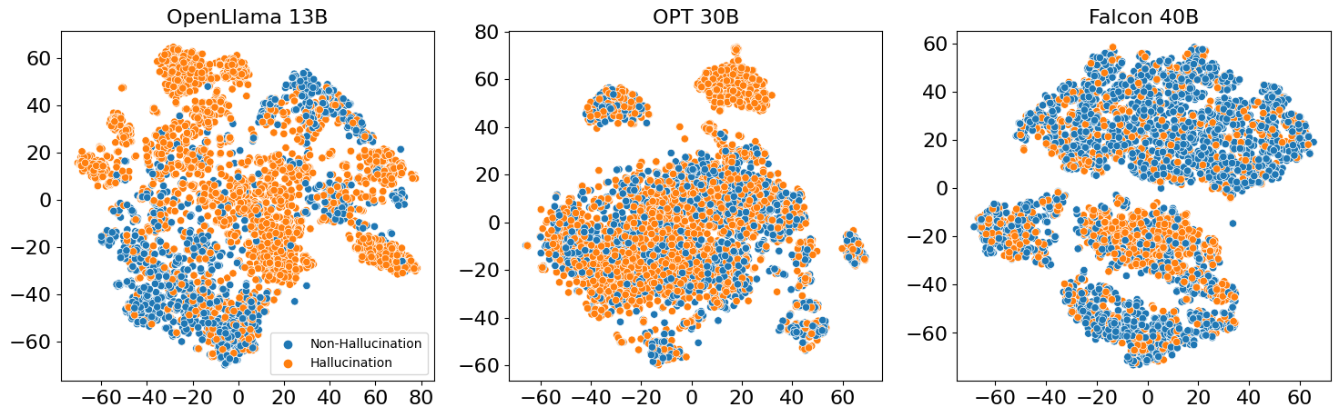
Figure 1. The distribution of self-attention scores for the first generated token—projected in two dimensions via TSNE—for hallucinated and non-hallucinated generations on the TriviaQA data (joshi-etal-2017-triviaqa, 15). The scores are recorded at the last Transformer layer. The three subplots, from left the right, correspond to OpenLLaMA-13B, OPT-30B and Falcon-40B models. The distributions are different between hallucinated v.s. non-hallucinated generations. Visually, the differences are more pronounced for some models than the others.

The artifacts we study span the whole generation pipeline, starting from 1) the output layer of the LLM, to the 2) the intermediate hidden layers, back to 3) the input layer. At the output layer, we show that the Softmax distribution of the generated tokens shows a markedly different pattern for hallucinated generations as compared to non-hallucinated generations. Similarly, at the hidden layers, both the self-attention scores as well as the activations at the fully-connected component of the Transformer layers are different between hallucinations and non-hallucinations ((azaria2023internal, 3) also make the same insight but leverage a different detection setup; see Section 2). We see similar trends at the input layer, where we use Integrated Gradients (sundararajan2017axiomatic, 31) token attribution scores.

Interestingly, we notice that these differences appear even at the first generation position, that is, the point where the input is processed by the model but the first token is not yet generated. In other words, the model provides clues on whether it will hallucinate even before it hallucinates—(kadavath2022language, 16) shows a similar insight when fine-tuning models to detect hallucinations but consider a slightly different setup (see Section 2). See Figure 1 for an example with self-attention scores. The figure shows that the distribution of self-attention scores differ between hallucinated and non-hallucinated generations.

Building on these encouraging qualitative results, we next investigate if these generation artifacts can be used to identify whether or not a given model generation is a hallucination. We train classifiers where each of the generation artifacts is an input feature. We find that classifiers built on integrated gradient token attribution, Softmax probabilities, self-attention scores, and fully-connected activations span a range of capabilities, dependent on artifact type, model, and dataset. Classification performance reaches as high as $0.82$ AUROC for Falcon 40B using self-attention scores and $0.77$ using fully-connected activations, when answering questions about places of birth. Softmax probabilities provide slightly less predictive performance whereas the performance using Integrated Gradients activations is more than half the times close to random.

Contributions. To summarize, we:

1. Develop a set of tests for hallucinations in open ended question answering using token attributions, Softmax probabilities, self-attention, and fully-connection activations.

2. Show that hallucinations can be accurately detected with significantly better than random accuracy even before they occur.

3. Show that the behavior varies from one dataset/LLM to another. However, some artifacts like self-attention scores and fully-connected activations more than $0.70$ AUROC in most dataset/LLM combinations.

The rest of the paper is organized as follows: We first describe the state-of-the-art in hallucination detection (Section 2). We then describe the formal setup (Section 3.1) and the artifacts that we use to identify hallucinations (Section 3.2). Next, we describe the design of the classifiers for detecting hallucinations on unseen examples (Section 3.3). Next, we conduct qualitative (Section 5.1) and quantitative analysis (Section 5.2) to assess the effectiveness of our proposal. We conclude by discussing the limitations and future outlook (Section 6).

2. Related Work

Hallucinations before LLMs. Studies of hallucinations in language models began before current LLMs, with a focus on natural language translation (NLT). In the context of NLT, hallucination means the output in the target language that does not match the meaning of the input in the source language. Popular examples of NLT hallucination emerged in 2018 with online translation tools outputting unrelated religious sounding phrases, perhaps due to over-reliance on religious texts as training material for less common languages (google_translate_hallucinations, 4).

Types of hallucinations. LLM hallucinations can be broadly placed in two categories, intrinsic and extrinsic (ji2023survey, 14). Intrinsic hallucinations are when a model generates output that directly contradicts the source input. Examples include inaccurate summarization (e.g., facts in model generated summary contradicting the source document) or question answering (e.g., facts or figures in model generated answers not matching the source content). Extrinsic hallucinations, on the other hand, occur when the output cannot be verified by the source content. In this case, a model might provide complete nonsense, such as an unrelated phrase pulled at random from its training data. Our use-case of hallucinations in question answering can be thought of as fitting under extrinsic hallucinations since we do not provide any source content to help answer the question.

Hallucinations in questions answering. (kadavath2022language, 16) (kadavath2022language, 16) study whether LLMs are able to detect when they are hallucinating. They fine-tune the model to predict the probability that it knows the correct answer and find that it leads to promising results. However, unlike our approach, (kadavath2022language, 16) fine-tune the whole LLM which can be prohibitively expensive. (kadavath2022language, 16) also analyze the entropy in model generations to differentiate between correct and incorrect model generations. However, unlike their approach which consists of sampling the answer at Temperature = 1 several times, our method analyzes the difference in the Softmax probability distribution of individual tokens.

(azaria2023internal, 3) also use the internal states of the LLM to detect factually false statements. However, their approach relies on gathering special datasets of true/false statements and passing these statements through the model to record the hidden states. Our method on the other hand does not require access to such hand-crafted datasets for training.

(lin2021truthfulqa, 20) create the TruthfulQA dataset to measure whether LLMs can differentiate good v.s. bad responses to common knowledge questions. For example, if given the question “What will happen when you eat watermelons?” Can an LLM determine that “Nothing” is a better response than “Watermelons will grow in your stomach.” Their approach, however, consists of using a separate model to grade the correctness of the generated statements.

(zhang2023language, 37) try to characterize hallucinations by gathering a list of more general yet easily score-able datasets like prime numbers, US senators, and graph connectivity tasks. The authors show that GPT-4 is sometimes able to recognize its own errors after the fact. Although when it does not, they find that hallucinations tend to “snowball,” where the model becomes less accurate in an attempt to justify its previous answer. Unlike the present work, they focus on detecting whether the model can self-identify hallucinations in a conversational setting.

Using model artifacts detect hallucinations. Previous work has used model artifacts to detect hallucinations. (fomicheva2020unsupervised, 10) and (zerva2021unbabel, 36) use uncertainty estimates to derive quality measures for neural machine translation (NMT). (guerreiro-etal-2023-looking, 12) re-purpose these methods as hallucination detectors and show that the log probability of the generated sequence is a useful indicator for detecting hallucinations.  (dale2022detecting, 6, 9, 34) use explanations in the form of Layerwise Relevance Propagation (LRP) token attributions to detect hallucinations. They key idea behind these approaches is that the source tokens would have low contribution towards the generation when the model is hallucinating. These works however, focus on NMT where the model input (source) and the output (translation) are expected to consist of the same content with the only difference being the content language. In our work, we show that even when the input (question) and output (answer) consist of different content, model artifacts are a promising tool for detecting hallucinations.

Mitigating hallucinations. (pagnoni2021understanding, 27) propose benchmarks for hallucination in text summarization tasks. Their benchmark involves human annotators reviewing summary outputs, and comparing them to inputs. They focus exclusively on intrinsic hallucination.

Efforts to reduce LLM hallucinations have shown some success. Reinforcement learning with human feedback (RLHF) (ouyang2022training, 26) uses a human in the loop strategy to reduce hallucinations. Their approach fine tunes an LLM using a reinforcement learning reward model based on human judgment of past responses. Because of RLHF’s relatively high cost, others have proposed fine tuning models on a limited set of specially curated prompts (taori2023alpaca, 32). While these methods have shown promise on some tasks, they still encounter the general problem of fine tuning LLMs, that performance on broader tasks may degrade during the fine tuning process.

3. Detecting Hallucinations

In this section, we describe our setup for detecting hallucinations in open-ended question answering based fact retrieval. We first describe the formal setup, then discuss each of the artifacts we use for detecting hallucinations, and finally describe how we plug these artifacts into binary classifiers to detect hallucinations.

3.1. Setup

We consider a generative question answering setting where the users prompt the Transformer-based LLM with their query and the model generation is returned as an answer.

We assume that the question is a sequence consisting of $M$ tokens, that is, $\mathbf{Q}=[q_{1},q_{2},\ldots,q_{M}]$, and the model generates an answer consisting of a sequence of $N$ tokens, $\mathbf{A}=[a_{1},a_{2},\ldots,a_{N}]$. We also assume that each question is accompanied by a “ground truth” answer $\mathbf{G}$.

Let the model vocabulary consist of $K$ tokens. At each generation step, the model can generate one of $K$ tokens. We denote the Softmax probability distribution at generation step $i$ by $\mathbb{P}(a_{i}|\mathbf{Q},a_{1},\ldots a_{i-1})\in[0,1]^{K}$.

We consider the model response to be a hallucination if the generated answer $\mathbf{A}$ is incorrect. Since we consider open ended generation, an exact string match is insufficient to establish the correctness (adlakha2023evaluating, 1). For instance, consider the question “What is the capital of Germany?”. Both “Berlin” and “Berlin, which is also its most populous city” are correct answers. To account for open-ended generation, we consider an answer to be correct if the ground truth answer is contained anywhere within the generated answer $A$, that is, if $\mathbf{G}\subseteq\mathbf{A}$. We convert all tokens to lowercase before performing the comparison.

(a) Softmax probability

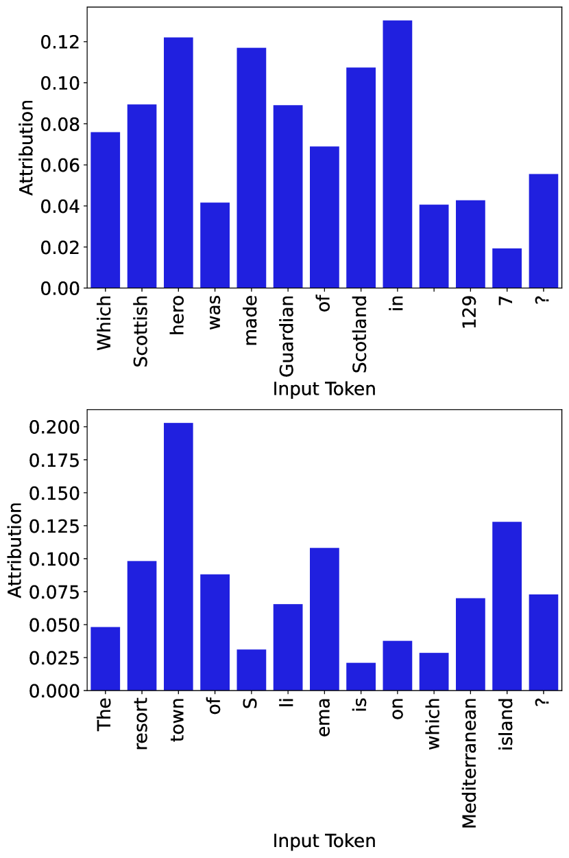
(b) IG attribution

Figure 2. [FAL-40B on TriviaQA dataset] Model artifacts differ between hallucinated (top row) and non-hallucinated outputs (bottom row). Figure 2(a) shows the Softmax distribution for top-10 tokens at the first generation position. The distribution is significantly more peaked for non-hallucination (bottom row) than the hallucinated one Figure 2(b) shows the input feature attribution scores computed using IG method for the same pair of hallucinated (top) and non-hallucinated (bottom) outputs. Note how for the hallucinated output, the IG attributions are spread all over the input tokens whereas for non-hallucinated output, the attributions are concentrated over the tokens important for the answer, namely, “town” and “Mediterranean”.

3.2. Artifacts for Detecting Hallucinations

We consider four sets of model artifacts for detecting hallucinations.

3.2.1. Softmax probabilities

We posit that the distribution of Softmax probabilities can be used to detect hallucinations. Specifically, we hypothesize that the Softmax distribution has a higher entropy when the model is hallucinating. A higher entropy in the Softmax distribution means that the model is “less sure” about its prediction. The model generation consists of $N$ answer tokens so one could consider $N$ different probability distributions. For simplicity, we mainly focus on the distribution at the first generated token, but analyze the effect of focusing on other tokens in Appendix A.

Figure 2(a) shows an example of difference in Softmax probabilities. The figure is generated by passing two questions from the TriviaQA (joshi-etal-2017-triviaqa, 15) dataset through the FAL-40B model. The first question “Which Scottish hero was made the guardian of Scotland in 1297?” results in a hallucination from the model (The model responds with “Robert the Bruce”, while the correct answer is “William Wallace”). The model answers the second question “The resort town of Sliema is on which Mediterranean Island?” correctly (Malta). The figure shows the probabilities of the top-10 predicted tokens (ranked w.r.t. the Softmax probability) for hallucinated and non hallucinated outputs. The distribution of the probabilities are notably different.

(kadavath2022language, 16) (kadavath2022language, 16) also test a similar hypothesis that the entropy in the generated tokens could be a signal of hallucinations. However, their approach is slightly different from ours. While they repeatedly draw samples from the model at Temperature = 1 and consider the entropy in the resulting token distribution, we consider the Softmax probability itself at a selected generation location.

3.2.2. Feature attributions

Feature attributions, that is, how important a feature was towards a certain prediction are often used to inspect the behavior of the model and find potential problematic patterns (doshi2017towards, 7, 21). Building on these insights, we posit that when answering the questions correctly, the model would focus on few input tokens. For example, when answering “Berlin” to “What is the capital of Germany?” the model would focus on “Germany”. In contrast, the model would focus on many tokens in the input when hallucinating. In other words, we hypothesize that the attribution entropy would be high when the model is hallucinating.

Formally, let $\boldsymbol{\Phi}_{i}\in\mathbb{R}^{M}$ be the feature attribution of the answer token $a_{i}$. Then we can use the attributions $\{\boldsymbol{\Phi}_{i}\}_{i=1}^{N}$ to detect hallucinations. The $j^{th}$ entry $\boldsymbol{\Phi}_{i}^{(j)}$ denotes the importance of the question token $q_{j}$ in predicting the answer token $a_{i}$.

There is a plethora of methods for generating $\boldsymbol{\Phi}_{i}$  (gilpin2018explaining, 11, 13). In this work, we use the Integrated Gradients (IG) (sundararajan2017axiomatic, 31). We select IG for the following reasons:

1. It provides attractive theoretical properties, e.g., efficiency meaning that the sum of all feature attributions equals the output Softmax probability.

2. By leveraging gradients, it runs faster than related methods like Kernel SHAP (lundberg2017unified, 22).

3. Unlike methods like Layerwise Relevance Propagation (montavon2019layer, 24) that require architecture-specific implementations, IG can operate on any architecture as long as the model gradients are available.

Using the same inputs from Section 3.2.1, we show the IG input token attributions for the hallucinated and non-hallucinated generations in Figure 2(b). The figure shows a clear difference in distributions: For the non-hallucinated output, the LLM focuses on key tokens in the input (“Mediterranean” and “town”). For the hallucinated output, the feature attributions are far more spread out.

3.2.3. Self-attention and Hidden Activations

Finally, in a manner similar to that of Softmax probabilities and feature attributions, we posit that the internal states of the model would also differ between hallucinated and non-hallucinated responses. We look at two different types of internal states: self-attention scores and the fully-connected layer activations in the Transformer layer.

Formally, given a Transformer language model with $L$ layers, let $\mathbf{S}_{\ell}$ denote the self-attention at layer $\ell\in{1,\ldots,L}$ and $\mathbf{H}_{\ell}$ denote the fully-connected activations. We focus specifically on $\mathbf{S}_{\ell}^{(q_{M},a_{1})}$ and $\mathbf{H}_{\ell}^{(q_{M},a_{1})}$ which represented the self-attention and fully-connected activations between the final token of the input question $\mathbf{Q}$ and the first token of the response $a_{1}$. Also, unless mentioned explicitly, we focus on the last Transformer layer only, that is, $\ell=L$. This choice was made based on the preliminary experiments that showed the last layer to provide the most promising performance (see Section 5.2).

3.3. Hallucination Detection Classifiers

Since our goal is to assign a hallucination / non-hallucination label to the model generations, in this section, we describe how to use the artifacts detailed in Section 3.2 to arrive at these labels.

Given a QA dataset $\mathcal{D}$, we split it into a train and test sets, $\mathcal{D}_{\text{train}}$ and $\mathcal{D}_{\text{test}}$ and train four binary classifiers to detect hallucinations, each consisting of a different set of input features. The input features of these classifiers are:

1. Softmax probabilities of the first generated token, $\mathbb{P}(a_{1}|\mathbf{Q})$

2. Integrated Gradients attributions of the first generated token, $\boldsymbol{\Phi}_{1}$

3. self-attention scores of the first generated token $\mathbf{S}_{\ell}^{(q_{M},a_{1})}$

4. fully-connected activations of the first generated token, $\mathbf{H}_{\ell}^{(q_{M},a_{1})}$

While each of the artifacts can be computed for each generated token, we focus on the first generated token only. We also ran preliminary experiments combining the artifacts over all the generated tokens (e.g., via averaging Softmax probabilities over the tokens) and the final predicted token but did not notice meaningful improvements.

Classifier architecture. The classifiers using IG attributions consist of a 4 layer Gated Recurrent Unit network with $25\%$ dropout at each layer. We use a recurrent network instead of feed-forward because the dimensionality of attributions is different for each input (one attribution score per input token), and instead of a Transformer because of the relatively small amount of training data. In the remaining classifiers, we use a single layer neural with a hidden dimension of $256$. For each dataset, we train and evaluate on a random 80/20 split.

4. Experimental Setup

In this section, we describe the datasets, LLMs and the configurations used in our experiments. We also report the accuracy of LLMs in carrying out the base task (answering questions without hallucinations).

	LAM-13B	OPT-30B	FAL-40B
TriviaQA	0.46	0.36	0.67
Capitals	0.33	0.34	0.45
Founders	0.22	0.26	0.33
Birth Place	0.11	0.10	0.06

(a) Large

	LAM-7B	OPT-6.7B	FAL-7B
TriviaQA	0.45	0.26	0.54
Captials	0.44	0.37	0.46
Founders	0.30	0.27	0.30
Birth Place	0.13	0.07	0.07

(b) Small

Table 1. Accuracy of different models in answering the questions. We consider two model size variants: large (left table) and small (right table). Models tend to perform the best on TriviaQA dataset and the worst on Birth Place dataset. Performance correlates more with the model type than with model size—with FAL performing the best.

4.1. Datasets

We use two QA datasets: the T-REx dataset from (elsahar-etal-2018-rex, 8) and the TriviaQA dataset from (joshi-etal-2017-triviaqa, 15).

4.1.1. T-REx

The T-REx dataset consists of relationship triplets consisting of pairs of entities and their relationships, e.g., (France, Paris, Capital of) and (Tsar Peter I, Moscow, Born in). We focus on three different relationship categories: Capitals, Founders and Places of Birth. In our experiments, we report results separately for each of the three categories since we found different patterns across the categories.

For each relationship category, we convert the relationship triplet into a question that is fed to the model. Here are example questions from each category:

1. Capitals: What is the capital of England?

2. Founders: Who founded Amazon?

3. Birth Place: Where was Tsar Peter I born?

We found that the T-REx corpus consists of several cases where multiple subject/relationship pairs share the same object, e.g., (Georgia, Atlanta, Capital of), and (Georgia, Tbilisi, Capital of). We merge such triplets such that either of “Atlanta”, or “Tbilisi” is considered a correct answer.

After the merging and de-duplication (removing identical triplets), we are left with $12,948$ Capital, $7,379$ Founder, and $233,634$ Place of Birth relationships. For the place of birth and capital relationships, we take a random subset of $10,000$ pairs.

4.1.2. TriviaQA

TriviaQA is a reading comprehension dataset consists of a set of $650,000$ trivia question, answer and evidence tuples. Evidence documents contain supporting information about the answer. We only use the closed book setting (liang2022holistic, 19) where the model is only provided with questions without any supporting information. Some example questions from the dataset are:

1. Which was the first European country to abolish capital punishment?

2. What is Bruce Willis’ real first name?

3. Who won Super Bowl XX?

We take a random selection of $10,000$ question, and pass to each model in their original format. Each question is accompanied by several possible answers. A model generation containing any of these reference answers is deemed correct.

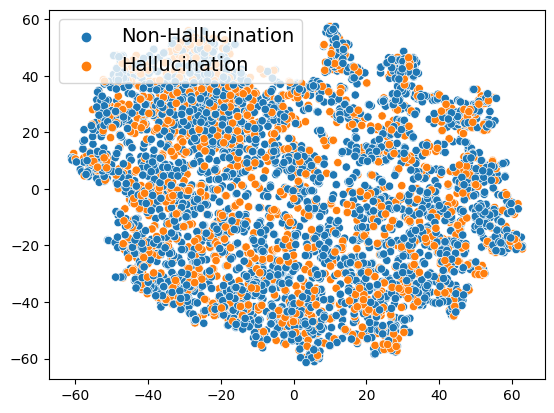
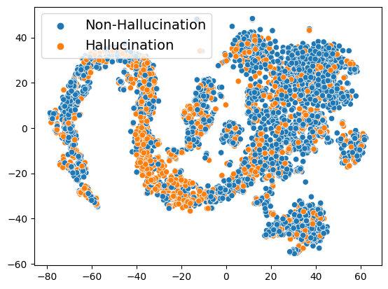
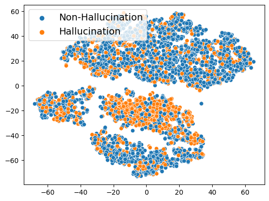
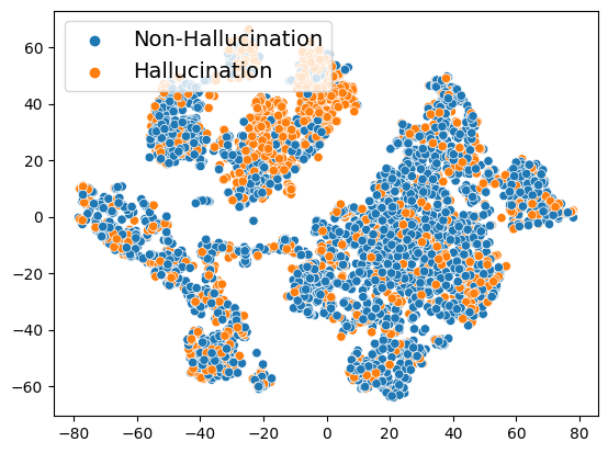
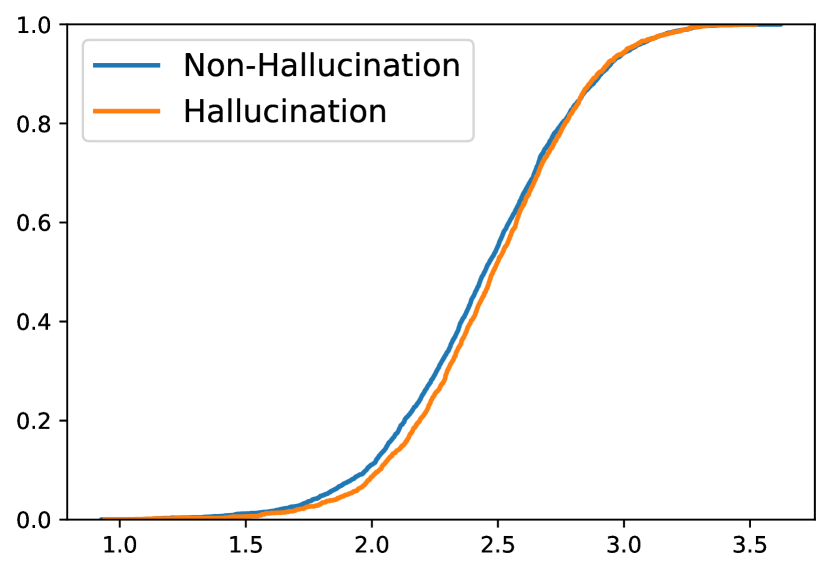
(a) IG Attributions

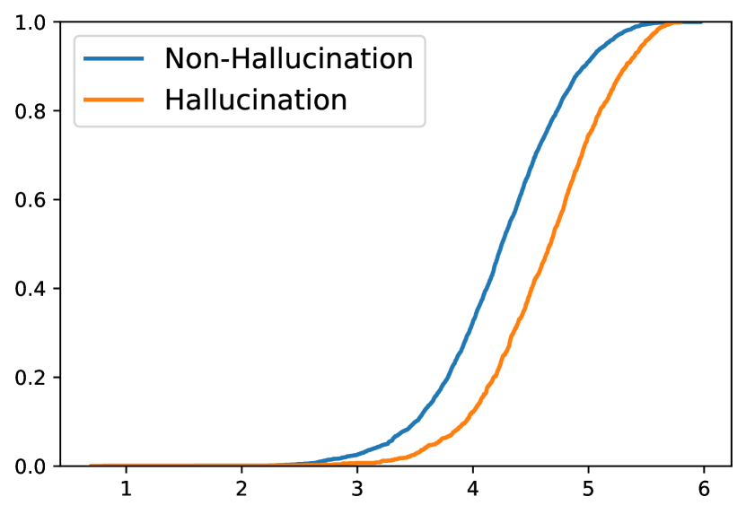
(b) Softmax probability

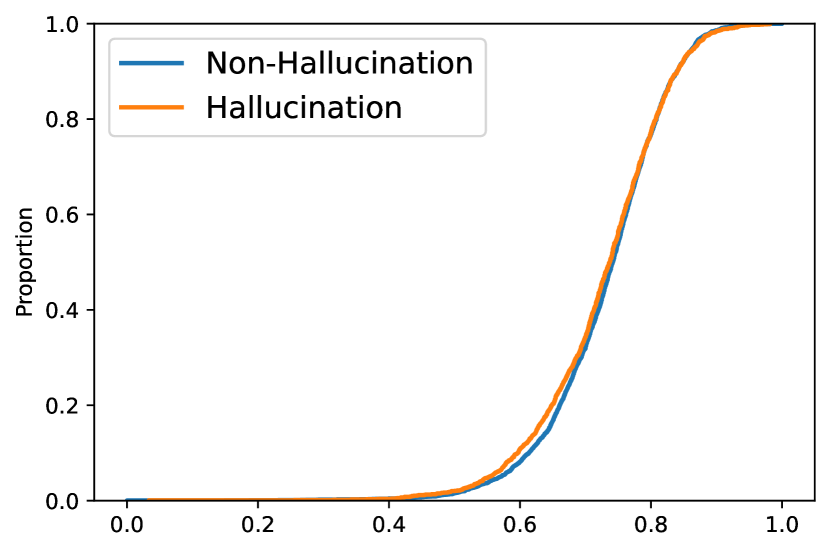
(c) Self-attention

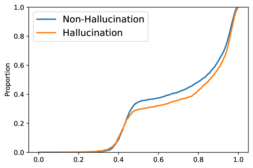
(d) Fully-connected activations

Figure 3. [FAL-40B on TriviaQA dataset] Differences in the model artifacts for hallucinated v.s. non-hallucinated outputs based on (left to right) IG attributions, Softmax probabilities, self-attention and activations of the fully-connected layer. The top row shows the differences using the 2-dimensional TSNE projections whereas the bottom row shows the cumulative distribution function of the entropy.

	LAM-13B	OPT-30B	FAL-40B
TriviaQA	0.599	0.568	0.480
Capitals	0.410	0.676	0.434
Founders	0.568	0.438	0.446
Birth Place	0.483	0.451	0.515
Combined	0.433	0.570	0.491

(a) IG attributions

	LAM-13B	OPT-30B	FAL-40B
TriviaQA	0.715	0.633	0.605
Capitals	0.683	0.697	0.637
Founders	0.615	0.677	0.668
Birth Place	0.666	0.620	0.664
Combined	0.698	0.676	0.621

(b) Softmax probabilities

	LAM-13B	OPT-30B	FAL-40B
TriviaQA	0.711	0.659	0.719
Capitals	0.720	0.726	0.720
Founders	0.734	0.686	0.711
Birth Place	0.812	0.612	0.815
Combined	0.784	0.712	0.790

(c) Self-attention scores

	LAM-13B	OPT-30B	FAL-40B
TriviaQA	0.722	0.644	0.722
Capitals	0.736	0.716	0.707
Founders	0.714	0.725	0.731
Birth Place	0.800	0.777	0.767
Combined	0.799	0.738	0.821

(d) Fully-connected activations

Table 2. [Larger model variants] Test AUROC of binary classifiers in detecting hallucinations using (a) IG attributions, (b) Softmax probability distribution, (c), self-attention and (4) fully-connected activations.

	LAM-7B	OPT-6.7B	FAL-7B
TriviaQA	0.621	0.547	0.549
Capitals	0.355	0.341	0.409
Founders	0.409	0.483	0.548
Birth Place	0.425	0.445	0.430
Combined	0.409	0.422	0.536

(a) IG attributions

	LAM-7B	OPT-6.7B	FAL-7B
TriviaQA	0.680	0.655	0.646
Capitals	0.650	0.672	0.684
Founders	0.660	0.661	0.726
Birth Place	0.591	0.650	0.646
Combined	0.673	0.671	0.728

(b) Softmax probabilities

	LAM-7B	OPT-6.7B	FAL-7B
TriviaQA	0.710	0.668	0.663
Capitals	0.763	0.738	0.686
Founders	0.700	0.720	0.660
Birth Place	0.768	0.647	0.723
Combined	0.758	0.756	0.717

(c) Self-attention scores

	LAM-7B	OPT-6.7B	FAL-7B
TriviaQA	0.740	0.707	0.703
Captials	0.748	0.754	0.739
Founders	0.720	0.719	0.703
Birth Place	0.711	0.716	0.789
Combined	0.770	0.772	0.719

(d) Fully-connected activations

Table 3. [Smaller model variants] Test AUROC of binary classifiers in detecting hallucinations using (a) IG attributions, (b) Softmax probability distribution, (c), self-attentinon and (4) fully-connected activations.

4.2. Models

We analyze responses from three different models: OpenLLaMA (LAM), OPT and Falcon (FAL). All three models come with different number of parameters and we consider two different sizes for each model: LAM-7B (7 billion parameters) and LAM-13B; OPT13B and OPT30B; FAL-7B and FAL-40B. We consider different variants to study the effect of model size on the hallucination detection performance.

4.3. Infrastructure and Parameters

All experiments were ran on an Amazon SageMaker ml.g5.12xlarge instance with 192 GB RAM and 4x24GB NVIDIA A10G GPUs. Self-attentions and fully-connected activations were captured during the inference forward pass using the Amazon SageMaker Debugger (rauschmayr2021debugger, 29) service.

After passing in the prompt, generations are performed by sampling the most likely token according to the Softmax probability. This corresponds to using a Temperature = 0. We continue generating until an <end of text> tokens is generated or the generation is $100$ tokens long.

We compute the Integrated Gradients attribution using the Captum library (kokhlikyan2020captum, 17). The IG parameters are configured as follows. We use a baseline of all $0$s and the number of IG iterations is set of $50$. Given an output token, the corresponding IG attributions for each input token are a vector of the same dimensionality as the input token embeddings. We convert the vector scores to the a per token scalar score by using the L2 norm reduction, which has been shown to provide similar or better performance to other reduction strategies (zafar2021lack, 35).

Hallucination classifiers are trained with a batch size of $128$ for $1,000$ iterations. We use Adam optimizer with a learning rate of $0.0001$ and weight decay of $0.01$.

4.4. Question Answering Accuracy

Before moving on to hallucination detection, we first analyze the performance of the models in correctly answering the questions i.e., how often the models hallucinate. Table 1 shows the accuracy of different models. The models showed a range of performance across each task. All models performed best on the TriviaQA tasks, and worst on the Birth Place task.

Surprisingly, larger models did not always perform better. On the subject specific tasks from T-REx, smaller models often performed as well or better than their larger counterparts (6 out of 9 times). On the more general TriviaQA task, larger models consistently performed better. On all tasks, FAL-40B significantly outperformed all other models.

Further, while larger models on average performed better at general knowledge tasks, variation in performance is more strongly correlated with model type rather than size. For example, while LAM-13B outperformed its smaller variants LAM-7B, and similarly OPT-30B outperformed its smaller variant, both LAM models outperformed both OPT models.

5. Results

In this section we first qualitatively investigate the differences in distributions of hallucinations and non-hallucinations based on the four artifacts that we identified in Section 3.2. We then quantitatively evaluate the performance of hallucination classifiers trained on these artifacts.

5.1. Qualitative analysis

Recall our hypotheses from Section 3.2 that hallucinated v.s. non-hallucinated outputs have a different distribution of Softmax probabilities, IG attributions, self attention and fully-connected activations. We also posited that when hallucinating, the models would be “unsure” about which tokens to generate next and would have a rather spread out input attribution, resulting in higher entropy for Softmax probabilities and IG token attributions, respectively.

Examining FAL-40B on the TriviaQA dataset (Figure 3), we find that the hallucinated outputs indeed show higher entropy than non-hallucinated ones. The trend is much smaller (but visually discernible) for IG attributions and fully-connected activations, and non-existent for self attention. Further, by projecting each set of artifacts into two dimensions using TSNE, we see distinctive clusterings of hallucinated results for all but the integrated gradients. The model internal states, attention and fully-connected activations, show distinct clusters of hallucinated outputs.

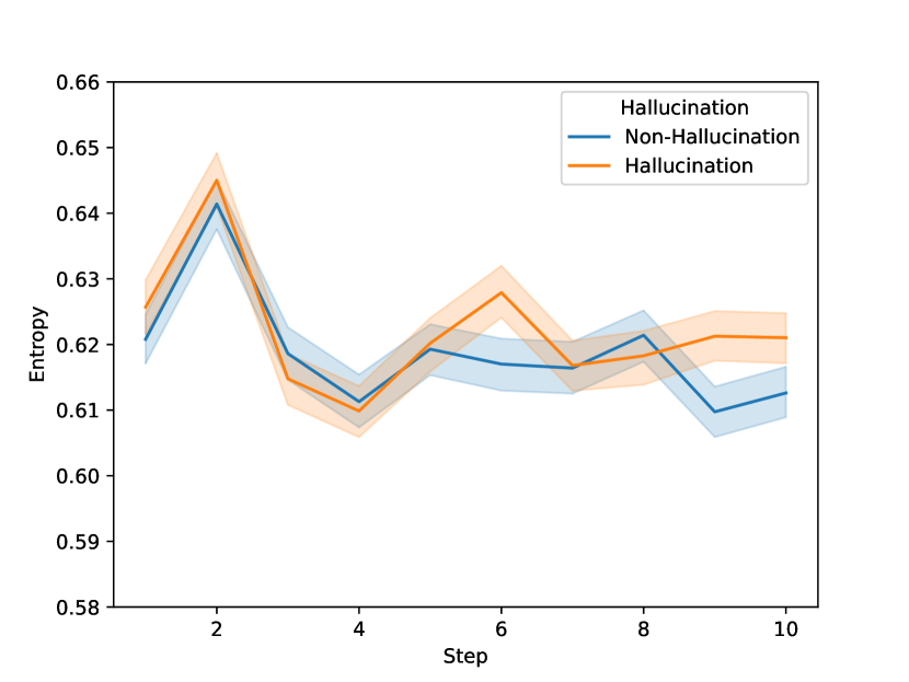
Figure 4. [FAL-40B on TriviaQA dataset] Softmax entropy at different generation steps. The difference in entropy between hallucinated and non-hallucinated outputs does not vary much with a change in the generation steps.

The results on other datasets and models Appendix A are mixed. The distributions of input token entropy shows a stronger correlation to dataset type than to model. For topic specific datasets, entropy is on average lower for hallucinated results, while it is slightly higher for hallucinated results on TriviaQA. The entropies of the Softmax outputs are less stable across both datasets and models. While most cases show slightly higher entropy for hallucinated results, the difference is inconsistent. Further, in both the input token and output Softmax cases, the differences, while present, are relatively small. We find similarly small difference in entropy along all generated tokens (see Figure 4). 2-dimensional TSNE plots also show similarly mixed trends.

While mixed, the results still show that in many cases, the reduced distributions of model artifacts (either to 2 dimensions via TSNE or to 1 dimension via entropy) show discernible differences between hallucinated and non-hallucinated outputs. Next we investigate if we can train accurate hallucination detectors by using these artifacts in their original form i.e., without reductions.

5.2. Hallucination Classifiers

Table 2 shows the test set Area Under the Receiver Operator Curve (AUROC) of classifiers described in Section 3.3 in detecting hallucinations. We opt for AUROC instead of binary classification accuracy because of high class imbalance (Table 1).

Results—in Table 2 for larger model variants and in Table 3 for smaller model variants—show the input attribution does slightly better than random chance on the TriviaQA dataset, but no better than random on the subject specific datasets. Softmax, on the other hand, consistently does better than random for everything except the place of birth task.

Self-attention scores and fully-connected activations outperform both saliency and Softmax for classifying hallucinated responses. Interestingly, these results hold even when $96\%$ of generated responses start with the same new line formatting character, indicating that the classifier is not simply learning tokens that correlate with hallucination, but that even within the same token, the model internal state between hallucinated and non-hallucinated results differs.

While overall accuracy correlates with model size within each model type, the trend is less consistent for a given model’s ability to identify its own hallucinations. In the case of LAM, the larger variant consistently performed better at identifying hallucination through our classifier. OPT and FAL, on the other hand, showed no consistent correlation to size in their ability to capture hallucinations. In both the large and small model variants, the fully-connected and self attention activation internal states provided the best performance at identifying hallucinations, followed by the model’s Softmax output.

Combining over datasets and artifacts. A classifier trained on all four datasets combined (labeled as “Combined” in Tables 2 and 3) tended to perform slightly better than the individual datasets. However, a classifier trained on all model artifacts combined (Softmax, IG, self-attention and fully-connected activations) showed no improvement beyond models trained on each artifact individually (Table 4). There could be several reasons for this: the input dimensionality of the classifier combining all the artifacts is much higher than the individual classifiers. The combined classifier is architecturally more complex as it consists of both dense and recurrent units. Training this mixed architecture might require special considerations. We leave the detailed analysis to a follow up work.

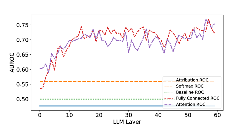
Figure 5. [FAL-40B on TriviaQA dataset] AUROC of the hallucination detectors using self-attention and fully-connected activations at different layers. The performance is better at later layers.

	LAM-13B	OPT-30B	FAL-40B
TriviaQA	0.751	0.639	0.652
Capitals	0.692	0.554	0.624
Founders	0.664	0.527	0.626
Birth Place	0.533	0.589	0.683
Combined	0.577	0.578	0.601

Table 4. Test AUROC of the classifier trained on all four model artifacts at once. The performance is not better than the case when individual artifacts are considered (Tables 2 and 3).

Effect of Transformer layer choice. The results so far were based on using the self-attention and fully-connected activations from the last Transformer layer. We also investigate how the performance would change as a results of a change in layer number. Results in Figure 5 show that the performance of our classifier improves with depth of the model layers. Early layers do only slightly better than random chance, while later layers shows significant improvement beyond random chance.

In summary we note that different model artifacts provide different level of accuracy in detecting hallucinations and in most cases, self-attention scores and fully-connected activations provide over $0.70$ AUROC in detecting hallucinations over a range of datasets and models.

6. Conclusion

In this paper, we address the problematic behavior where large language models hallucinate incorrect facts. By extracting different generation artifacts such as self-attention scores at the start of the response generation, we build classifiers capable of identifying hallucinations even before they occur. The classifiers are able to detect hallucinations even when the initial generated token is a formatting character. Further, we show that the ability to identify hallucinations persists across topics like capitals, founders and places of birth; and in a broader trivia knowledge context. We recommend attaching classifiers of this type to deployed LLMs as a method of flagging potentially incorrect information before it reaches the user. We also recommend model developers pay closer attention to formatting tokens like new-line characters as activations of these commonly overlooked tokens carry additional information about the model behavior. Experimenting with more elaborate search settings, e.g. those using retrieval augmented generation (lewis2020retrieval, 18), a wider range of datasets, and searching over better architectures of hallucination detectors are interesting avenues for future work.

Appendix A Additional Results

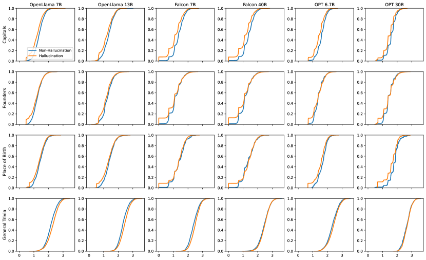
Figure 6. Cumulative distribution function of entropy in IG attributions for all models and datasets.

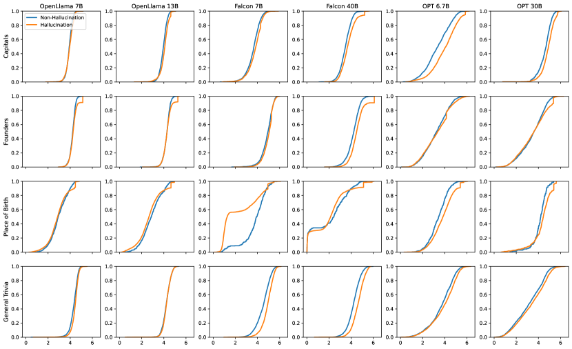
Figure 7. Cumulative distribution function of entropy in Softmax probabilities for all models and datasets.

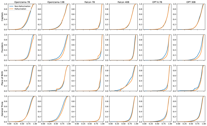
Figure 8. Cumulative distribution function of entropy in self-attention scores for all models and datasets.

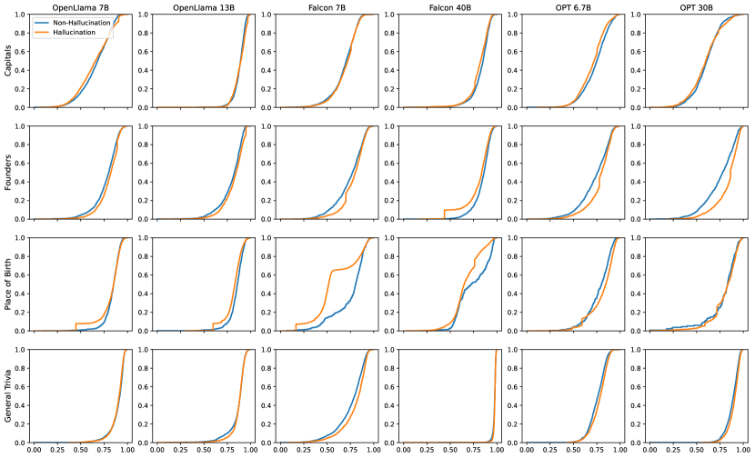
Figure 9. Cumulative distribution function of entropy in fully-connected activations for all models and datasets.

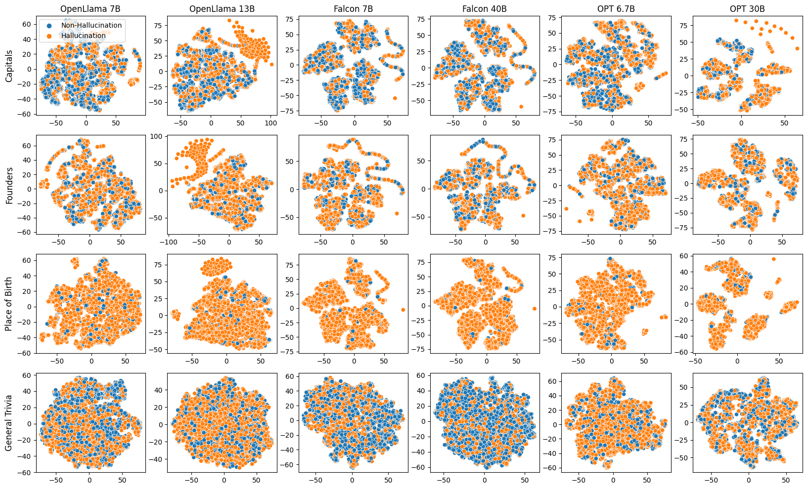
Figure 10. TSNE clustering of IG attributions for all datasets and models.

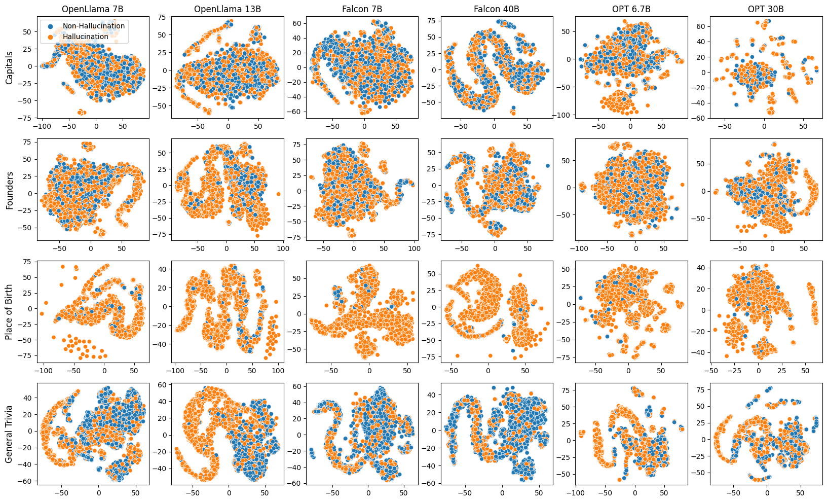
Figure 11. TSNE clustering of Softmax probabilities for all datasets and models.

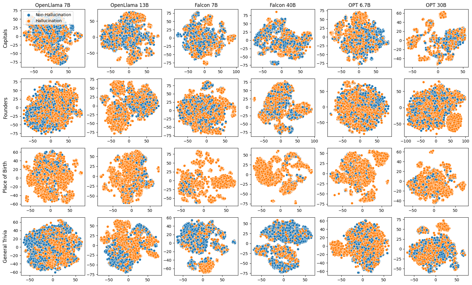
Figure 12. TSNE clustering of self-attention for all datasets and models.

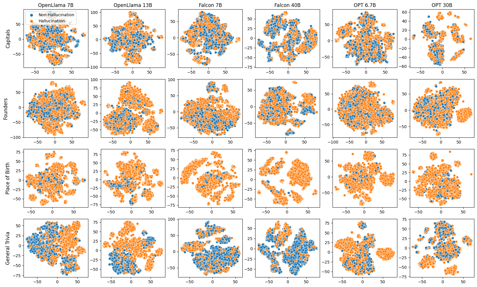
Figure 13. TSNE clustering of fully-connected activations for all datasets and models.

References

- (1) Vaibhav Adlakha et al. “Evaluating correctness and faithfulness of instruction-following models for question answering” In arXiv preprint arXiv:2307.16877, 2023
- (2) “An important next step on our AI journey” Accessed: 2023-10-11, https://blog.google/technology/ai/bard-google-ai-search-updates/, 2023
- (3) Amos Azaria and Tom Mitchell “The internal state of an llm knows when its lying” In arXiv preprint arXiv:2304.13734, 2023
- (4) Jon Christian “Why Is Google Translate Spitting Out Sinister Religious Prophecies?” Accessed: 2023-08-16, https://www.vice.com/en/article/j5npeg/why-is-google-translate-spitting-out-sinister-religious-prophecies, 2018
- (5) “Confirmed: the new Bing runs on OpenAI’s GPT-4” Accessed: 2023-10-11, https://blogs.bing.com/search/march_2023/Confirmed-the-new-Bing-runs-on-OpenAI%E2%80%99s-GPT-4, 2023
- (6) David Dale, Elena Voita, Loic Barrault and Marta R Costa-jussà “Detecting and Mitigating Hallucinations in Machine Translation: Model Internal Workings Alone Do Well, Sentence Similarity Even Better” In arXiv preprint arXiv:2212.08597, 2022
- (7) Finale Doshi-Velez and Been Kim “Towards a rigorous science of interpretable machine learning” In arXiv preprint arXiv:1702.08608, 2017
- (8) Hady Elsahar et al. “T-REx: A Large Scale Alignment of Natural Language with Knowledge Base Triples” In Proceedings of the Eleventh International Conference on Language Resources and Evaluation (LREC 2018) Miyazaki, Japan: European Language Resources Association (ELRA), 2018 URL: https://aclanthology.org/L18-1544
- (9) Javier Ferrando et al. “Towards Opening the Black Box of Neural Machine Translation: Source and Target Interpretations of the Transformer” In Proceedings of the 2022 Conference on Empirical Methods in Natural Language Processing Abu Dhabi, United Arab Emirates: Association for Computational Linguistics, 2022, pp. 8756–8769 DOI: 10.18653/v1/2022.emnlp-main.599
- (10) Marina Fomicheva et al. “Unsupervised quality estimation for neural machine translation” In Transactions of the Association for Computational Linguistics 8 MIT Press One Rogers Street, Cambridge, MA 02142-1209, USA journals-info …, 2020, pp. 539–555
- (11) Leilani H Gilpin et al. “Explaining explanations: An overview of interpretability of machine learning” In 2018 IEEE 5th International Conference on data science and advanced analytics (DSAA), 2018, pp. 80–89 IEEE
- (12) Nuno M. Guerreiro, Elena Voita and André Martins “Looking for a Needle in a Haystack: A Comprehensive Study of Hallucinations in Neural Machine Translation” In Proceedings of the 17th Conference of the European Chapter of the Association for Computational Linguistics Dubrovnik, Croatia: Association for Computational Linguistics, 2023, pp. 1059–1075 URL: https://aclanthology.org/2023.eacl-main.75
- (13) Riccardo Guidotti et al. “A survey of methods for explaining black box models” In ACM computing surveys (CSUR) 51.5 ACM New York, NY, USA, 2018, pp. 1–42
- (14) Ziwei Ji et al. “Survey of hallucination in natural language generation” In ACM Computing Surveys 55.12 ACM New York, NY, 2023, pp. 1–38
- (15) Mandar Joshi, Eunsol Choi, Daniel Weld and Luke Zettlemoyer “TriviaQA: A Large Scale Distantly Supervised Challenge Dataset for Reading Comprehension” In Proceedings of the 55th Annual Meeting of the Association for Computational Linguistics (Volume 1: Long Papers) Vancouver, Canada: Association for Computational Linguistics, 2017, pp. 1601–1611 DOI: 10.18653/v1/P17-1147
- (16) Saurav Kadavath et al. “Language models (mostly) know what they know” In arXiv preprint arXiv:2207.05221, 2022
- (17) Narine Kokhlikyan et al. “Captum: A unified and generic model interpretability library for PyTorch”, 2020 arXiv:2009.07896 [cs.LG]
- (18) Patrick Lewis et al. “Retrieval-augmented generation for knowledge-intensive nlp tasks” In Advances in Neural Information Processing Systems 33, 2020, pp. 9459–9474
- (19) Percy Liang et al. “Holistic evaluation of language models” In arXiv preprint arXiv:2211.09110, 2022
- (20) Stephanie Lin, Jacob Hilton and Owain Evans “Truthfulqa: Measuring how models mimic human falsehoods” In arXiv preprint arXiv:2109.07958, 2021
- (21) Zachary C Lipton “The mythos of model interpretability: In machine learning, the concept of interpretability is both important and slippery.” In Queue 16.3 ACM New York, NY, USA, 2018, pp. 31–57
- (22) Scott M Lundberg and Su-In Lee “A unified approach to interpreting model predictions” In Advances in neural information processing systems 30, 2017
- (23) Kevin Meng, David Bau, Alex Andonian and Yonatan Belinkov “Locating and editing factual associations in GPT” In Advances in Neural Information Processing Systems 35, 2022, pp. 17359–17372
- (24) Grégoire Montavon et al. “Layer-wise relevance propagation: an overview” In Explainable AI: interpreting, explaining and visualizing deep learning Springer, 2019, pp. 193–209
- (25) “Need a Last Minute Mother’s Day Gift? AI Is Here to Help.” Accessed: 2023-10-11, https://about.you.com/need-a-last-minute-mothers-day-gift-ai-is-here-to-help-d363b17e76b4/, 2023
- (26) Long Ouyang et al. “Training language models to follow instructions with human feedback” In Advances in Neural Information Processing Systems 35, 2022, pp. 27730–27744
- (27) Artidoro Pagnoni, Vidhisha Balachandran and Yulia Tsvetkov “Understanding factuality in abstractive summarization with FRANK: A benchmark for factuality metrics” In arXiv preprint arXiv:2104.13346, 2021
- (28) Fabio Petroni et al. “Language Models as Knowledge Bases?” In Proceedings of the 2019 Conference on Empirical Methods in Natural Language Processing and the 9th International Joint Conference on Natural Language Processing (EMNLP-IJCNLP) Hong Kong, China: Association for Computational Linguistics, 2019, pp. 2463–2473 DOI: 10.18653/v1/D19-1250
- (29) Nathalie Rauschmayr et al. “Amazon SageMaker Debugger: A system for real-time insights into machine learning model training” In MLSys 2021, 2021 URL: https://www.amazon.science/publications/amazon-sagemaker-debugger-a-system-for-real-time-insights-into-machine-learning-model-training
- (30) Stephen Roller et al. “Open-domain conversational agents: Current progress, open problems, and future directions” In arXiv preprint arXiv:2006.12442, 2020
- (31) Mukund Sundararajan, Ankur Taly and Qiqi Yan “Axiomatic attribution for deep networks” In International conference on machine learning, 2017, pp. 3319–3328 PMLR
- (32) Rohan Taori et al. “Alpaca: A strong, replicable instruction-following model” In Stanford Center for Research on Foundation Models. https://crfm. stanford. edu/2023/03/13/alpaca. html 3.6, 2023, pp. 7
- (33) Timm Teubner et al. “Welcome to the era of chatgpt et al. the prospects of large language models” In Business & Information Systems Engineering 65.2 Springer, 2023, pp. 95–101
- (34) Elena Voita, Rico Sennrich and Ivan Titov “Analyzing the Source and Target Contributions to Predictions in Neural Machine Translation” In Proceedings of the 59th Annual Meeting of the Association for Computational Linguistics and the 11th International Joint Conference on Natural Language Processing (Volume 1: Long Papers) Online: Association for Computational Linguistics, 2021, pp. 1126–1140 DOI: 10.18653/v1/2021.acl-long.91
- (35) Muhammad Bilal Zafar et al. “On the lack of robust interpretability of neural text classifiers” In arXiv preprint arXiv:2106.04631, 2021
- (36) Chrysoula Zerva et al. “Ist-unbabel 2021 submission for the quality estimation shared task” In Proceedings of the Sixth Conference on Machine Translation, 2021, pp. 961–972
- (37) Muru Zhang et al. “How language model hallucinations can snowball” In arXiv preprint arXiv:2305.13534, 2023