Fundamental charges for dual-unitary circuits

Abstract

Dual-unitary quantum circuits have recently attracted attention as an analytically tractable model of many-body quantum dynamics. Consisting of a 1+1D lattice of 2-qudit gates arranged in a ‘brickwork’ pattern, these models are defined by the constraint that each gate must remain unitary under swapping the roles of space and time. This dual-unitarity restricts the dynamics of local operators in these circuits: the support of any such operator must grow at the effective speed of light of the system, along one or both of the edges of a causal light cone set by the geometry of the circuit. Using this property, it is shown here that for 1+1D dual-unitary circuits the set of width-$w$ conserved densities (constructed from operators supported over $w$ consecutive sites) is in one-to-one correspondence with the set of width-$w$ solitons - operators which, up to a multiplicative phase, are simply spatially translated at the effective speed of light by the dual-unitary dynamics. A number of ways to construct these many-body solitons (explicitly in the case where the local Hilbert space dimension $d=2$) are then demonstrated: firstly, via a simple construction involving products of smaller, constituent solitons; and secondly, via a construction which cannot be understood as simply in terms of products of smaller solitons, but which does have a neat interpretation in terms of products of fermions under a Jordan-Wigner transformation. This provides partial progress towards a characterisation of the microscopic structure of complex many-body solitons (in dual-unitary circuits on qubits), whilst also establishing a link between fermionic models and dual-unitary circuits, advancing our understanding of what kinds of physics can be explored in this framework.

1 Introduction

Over the last decade, a number of models have been identified in the framework of local 1+1D brickwork quantum circuits that appear to be both quantum chaotic and partially solvable, heralding a rare opportunity to obtain sharp analytical results in chaotic many-body quantum systems. Perhaps the prototypical example of such a model is that of random unitary circuits [1, 2, 3, 4, 5], for which it was shown that out-of-time-order correlators (OTOCs) and the spectral form factor - amongst a number of other interesting dynamical quantities - are not only exactly calculable but also quantum chaotic, with a ballistic growth of generic local operators revealed by the OTOC [2, 3] and random-matrix level statistics revealed by the spectral form factor [5].

These calculations, however, require averaging over many realisations of the random circuit, and have exactness only in the limit of a large local Hilbert space dimension. These conditions can be circumvented in the model of dual-unitary circuits (DUCs), where the gates forming the circuit are unitary in both the time direction and the spatial direction of the circuit [6, 7, 8, 9, 10, 11, 12, 13, 14, 15, 16, 17, 18, 19, 20, 21, 22, 23, 24, 25, 26, 27, 28, 29, 30, 31, 32, 33, 34, 35, 36, 37] (see Section 2.2). This property can then be exploited to calculate the spectral form factor [7] and OTOCs [8], without requiring any averaging (for OTOCs) and without requiring a large local Hilbert space dimension. It is now also generally accepted that generic DUCs exhibit ‘maximal’ chaos, with a spectral form factor that matches the prediction of random matrix theory shown in Ref. [7], and a maximal butterfly velocity and exponential decay of the OTOC inwards from the edge of the strict causal light cone (enforced by the geometry of the circuit) shown in Ref. [8]. They have also been shown to be hard to classically simulate, in general [35].

Remarkably, the analytical tractability of these circuits extends well beyond calculations of OTOCs and the spectral form factor; for instance, correlation functions of local observables [6] and state [15, 16, 17, 18, 19, 20, 4] and operator [21, 22] entanglement entropies are all analytically accessible in DUCs, as well as there existing a class of ‘solvable’ matrix product states for which the time evolution of local observables under any dual-unitary dynamics is exactly calculable [17]. Again, calculation of these quantities for generic dual-unitary circuits often reveals ergodic behaviour (such as the exponential decay of local correlation functions [6]), and accordingly DUCs have been used to prove many aspects of thermalisation from first principles [23, 24, 25, 26]. They have been used to obtain exact results on the use of the Hayden-Preskill protocol to recover quantum information (with it being analytically demonstrable that they dynamically realise perfect decoding) [27], and were also the first non-random Floquet spin model shown to be treatable by entanglement membrane theory [28]. Much of this tractability also survives under the addition of measurements and non-unitarity (allowing the study of measurement-induced phase transitions in the context of these models) [29, 30, 31, 32, 33], under weak unitary perturbations away from dual-unitarity [38, 39], and in a recently introduced hierarchical generalisation of dual-unitarity [40, 41, 42, 43].

Despite primarily attracting attention as a solvable model of ergodic dynamics, however, DUCs are also capable - when finely tuned - of realising non-ergodic dynamics. In particular, they are capable of hosting solitons: local operators which, up to a multiplicative phase, are simply spatially translated at the effective speed of light (i.e. along an edge of the causal light cone) by the dual-unitary dynamics [22]. Dynamical quantities in DUCs with solitons display hallmarks of non-ergodicity - the level statistics may become Poissonian (see numerical results in the Supplementary Material of Ref. [9]), and correlation functions pertaining to the solitons will not decay [6, 9]. Moreover, an exponential number of conserved quantities can be constructed from each soliton [22]. Notably, however, the dynamics of solitons is rather atypical. In a many-body quantum system undergoing some ‘generic’ unitary dynamics, localised densities of conserved charge will typically diffuse and become ‘mixed in’ with nonconserved operators (such as in random unitary circuits [44, 45]). In contrast, solitons do not diffuse (the number of sites over which they are supported remains strictly constant) nor mix with other operators (or even other solitons), in that they do not produce any non-conserved operator density under the dynamics of the circuit.

It has previously been shown that, in 1+1D brickwork dual-unitary circuits, the existence of a conserved quantity formed from a sum over $n$ of $2n$-site spatial translations of some finite range operator also implies the existence of a soliton with unit phase [22]. In this work, we extend on this result by showing a similar one-to-one correspondence between a more general class of conserved quantities (we allow them to be inhomogeneous, by allowing for variation in the finite-range operator over the course of the sum) and solitons with complex phases. Specifically, in Section 3 we prove a more formal version of the following theorem.

Theorem 1.

Fundamental charges for DUCs (informal). Take a $1$D chain of local quantum systems. If a quantity formed from a linear combination of finite-range operators (i.e. each with non-trivial support over some finite number - say $w$ - of neighbouring sites) is conserved by a $1+1$D brickwork dual unitary circuit acting on the chain, then it can be broken down into a linear combination of conserved quantities generated by the solitons (which are finite sized, also with support over at most $w$ neighbouring sites) of the circuit. In the thermodynamic limit ($L\rightarrow\infty$), a result in the converse direction holds - a conserved quantity can be constructed from each soliton - giving a one-to-one correspondence between solitons and conserved quantities (see Remark 1).

Our belief is that this adds to the growing understanding of operator dynamics and non-ergodicity in dual-unitary many-body quantum systems, and also strengthens the sense in which solitons can be seen as fundamental charges for these systems. In essence, given a conserved quantity in a dual-unitary circuit, one only needs to know that it is formed from a linear combination of finite-range operators in order to know that it can be decomposed in terms of solitons.

The paper is structured as follows. In Section 2, we recap the model of DUCs, with a focus on solitons and conserved densities. In Section 3, our main results are presented, including a proof of the aforementioned correspondence between solitons and conserved densities (Theorem 1). In Section 4, the structure of many-body solitons in DUCs is considered (which are encompassed by Theorem 1), and we show that these can be constructed from smaller fermionic and solitonic constituent quantities. In Section 5, the results are recapped and directions for future work are discussed.

2 Dual-unitary circuits

2.1 Local 1+1D quantum circuits

The model which will be studied here is that of a brickwork 1+1D local unitary quantum circuit. The spatial part of this model consists of a $1$D geometry of $2L$ sites arranged on an integer lattice with periodic boundary conditions, $x\in\mathbb{Z}_{2L}$. We will often want to deal with sets of sites of the same parity, and so to facilitate this we introduce a notation

$$\mathbb{E}_{x}=\{e\in\mathbb{N}\;|\;e\leq x,\;e=0\mod 2\},$$ (1)

and

$$\mathbb{O}_{x}=\{o\in\mathbb{N}\;|\;o\leq x,\;o=1\mod 2\},$$ (2)

to denote the sets of even and odd positive integers in the interval $\left[1,x\right]$. To each site we associate a local Hilbert space $\mathcal{H}_{1}=\mathbb{C}^{d}$, such that the Hilbert space of the whole system is $\mathcal{H}_{2L}=\mathcal{H}_{1}^{\otimes 2L}$; in other words, we have a chain of $2L$ $d$-dimensional qudits.

For the temporal part of the model we define a Floquet operator, $\mathbb{U}\in\textrm{End}(\mathcal{H}_{2L})$, which acts on the chain of qudits as

$$\mathbb{U}=\Pi_{2L}V^{\otimes L}\Pi_{2L}^{-1}U^{\otimes L}=\;\;\;\includegraphics[width=173.44534pt,valign={c}]{floquetoperator.png}\;\;,$$ (3)

where

$$U=\;\;\;\includegraphics[width=30.35657pt,valign={c}]{U.png}\;\;,\quad V=\;\;\;\includegraphics[width=30.35657pt,valign={c}]{V.png}\;\;\quad\in\textrm{End}(\mathcal{H}_{1}\otimes\mathcal{H}_{1}),$$ (4)

are some 2-qudit unitary gates, and where we have introduced an $l$-site periodic one-site translation operator,

$$\Pi_{l}\ket{i_{1}}\otimes...\otimes\ket{i_{l}}=\ket{i_{2}}\otimes...\otimes\ket{i_{l}}\otimes\ket{i_{1}},$$ (5)

with the states $\{\ket{i};i=1,...,d\}$ forming a complete orthonormal basis for $\mathcal{H}_{1}$. Note that we are considering a (spatially) homogeneous circuit, so the Floquet operator is invariant under spatial translations by two sites,

$$\Pi_{2L}^{2}\mathbb{U}\Pi_{2L}^{-2}=\mathbb{U},$$ (6)

which manifests in parity effects that motivate the $\mathbb{O}$ and $\mathbb{E}$ notation introduced above.

A circuit enacting some unitary evolution for some time $t$ can then be constructed by taking $t$ sequential applications of the Floquet operator (so, save for the variation between the even and odd layers ($U\neq V$ in general), the circuit is also temporally homogeneous), i.e.

$$\mathcal{U}(t)=\mathbb{U}^{t}.$$ (7)

This gives us a brickwork 1+1D local quantum circuit, as shown in Fig. 1. The structure of the Floquet operator enforces periodic boundary conditions on our chain; we have a $1$D ring topology.

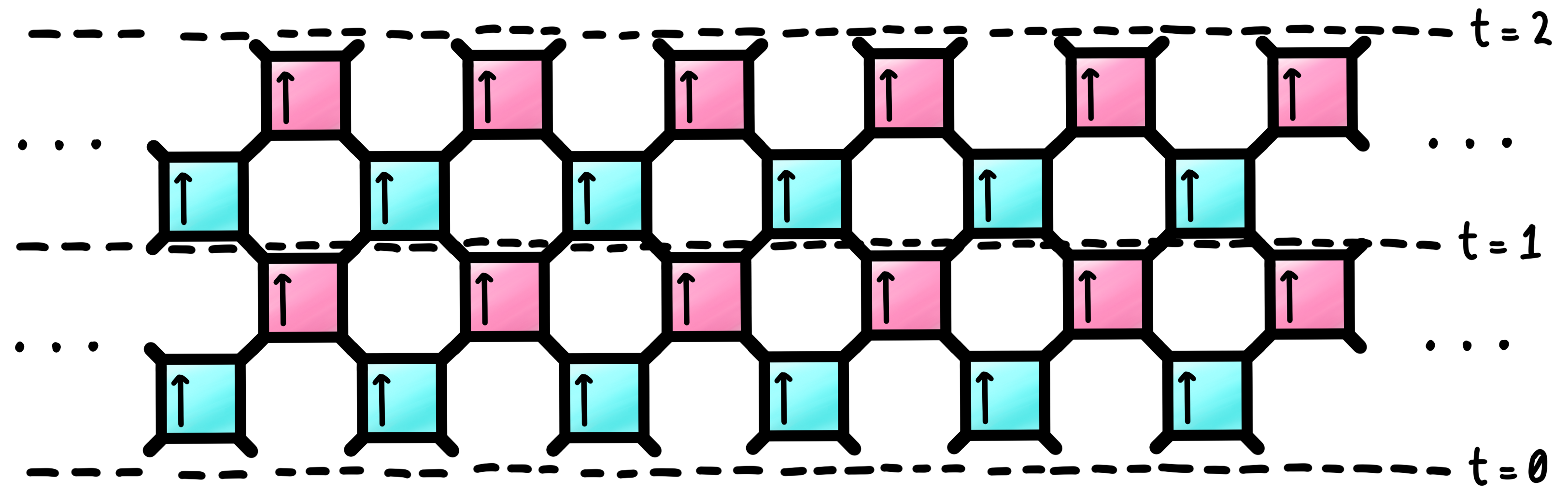
Figure 1: A brickwork circuit shown for two time steps, $t=2$, consisting of two Floquet periods, i.e. two sequential applications of the Floquet operator $\mathbb{U}$.

We will be primarily interested in the dynamics of ‘local’ (we use the term local quite loosely here; we will be considering operators which act non-trivially on a connected region of consecutive sites of length $\leq L$, i.e. half the length of the chain, $2L$) operators under the Floquet operator $\mathbb{U}$. To differentiate these operators from those generating the dynamics ($U$, $V$, $\mathbb{U}$) we will use bold font, representing some local operator on $l$ sites by $\bm{q}\in\mathcal{A}_{l}$, where $\mathcal{A}_{l}$ is the algebra of all matrices acting on $\mathcal{H}_{1}^{\otimes l}$. We will use $\bm{q}_{x}\in\mathcal{A}_{2L}$ to denote an operator which acts as identity on all sites except the site $x$, where it acts as the single-qudit operator $\bm{q}\in\mathcal{A}_{1}$. We can then generalise this notation to represent more extensive operators: $\bm{q}_{x,y}\in\mathcal{A}_{2L}$ denotes the $2$-qudit operator $\bm{q}\in\mathcal{A}_{2}$ acting on the sites $x$ and $y$; $\bm{q}_{x,...,x+w-1}\in\mathcal{A}_{2L}$ denotes the width-$w$ operator $\bm{q}\in\mathcal{A}_{w}$ acting on the connected region of the chain $\mathcal{R}=\left[x,x+w-1\right]\subseteq\mathbb{Z}_{2L},\;|\mathcal{R}|=w$. Throughout this work we will almost always want to assume, when talking about some operator $\bm{q}_{x,...,y}$ acting over a region of the chain $[x,y]$, that $\tr_{x}(\bm{q}_{x,...,y})=\tr_{y}(\bm{q}_{x,...,y})=0$ (i.e. the operator is strictly traceless at the boundary sites of its region of non-trivial support). Accordingly, we introduce the notation

$$\bar{\mathcal{A}}_{w}=\left\{\bm{a}\in\mathcal{A}_{w}|\tr_{0}(\bm{a}_{0,...,w-1})=\tr_{w-1}(\bm{a}_{0,...,w-1})=0\right\},$$ (8)

to explicitly pick out such operators.

2.2 Dual-unitaries

We enforce a constraint on our model: the local gates $U$ and $V$ must not only be unitary, in that $UU^{\dagger}=U^{\dagger}U=\mathds{1}$ and $VV^{\dagger}=V^{\dagger}V=\mathds{1}$, but also dual-unitary, in that the dual-gates, defined via a reshuffling of indices like so

$$\bra{i}\otimes\bra{j}\tilde{U}\ket{k}\otimes\ket{l}=\bra{l}\otimes\bra{j}U\ket{k}\otimes\ket{i},$$ (9)

are also unitary, $\tilde{U}\tilde{U}^{\dagger}=\tilde{U}^{\dagger}\tilde{U}=\mathds{1}$ and $\tilde{V}\tilde{V}^{\dagger}=\tilde{V}^{\dagger}\tilde{V}=\mathds{1}$. This can be thought of as enforcing unitarity in the spatial direction of our 1+1D circuit (in contrast to the standard notion of unitarity in time, represented by $UU^{\dagger}=U^{\dagger}U=\mathds{1}$), which can be illustrated diagrammatically like so,

$$\includegraphics[width=30.35657pt,valign={c}]{DU1.png}\;\;\;=\;\;\;\includegraphics[width=30.35657pt,valign={c}]{ducontractionR.png}\;\;\;,\;\;\;\includegraphics[width=30.35657pt,valign={c}]{DU2.png}\;\;\;=\;\;\;\includegraphics[width=30.35657pt,valign={c}]{ducontractionL.png}\;\;\;,$$ (10)

where we are using the convention from [34] that a darker shade represents complex conjugation (i.e. $\includegraphics[width=13.00806pt,valign={c}]{Ustar.png}=U^{*}$), and flipping the arrow represents transposition (i.e $\includegraphics[width=13.00806pt,valign={c}]{Utranspose.png}=U^{T}$), such that $\includegraphics[width=13.00806pt,valign={c}]{Udag.png}=U^{\dagger}$.

In [34], it was noted that dual-unitaries have the following property:

Property 1.

Dual unitaries map any single-site traceless operator into a linear combination of operators that are necessarily traceless on the neighbouring site. That is, for a quantity $\bm{a}\in\mathcal{A}_{1},\;\tr(\bm{a})=0$, initialised on a site $x$ and then acted upon by a dual-unitary gate $U$ coupling sites $x$ and $y$, the trace of $U\bm{a}_{x}U^{\dagger}$ is vanishing on site $y$,

$$\tr_{y}(U\bm{a}_{x}U^{\dagger})=\;\;\;\includegraphics[width=39.0242pt,valign={c}]{property1a.png}\;\;\;=\;\;\;\includegraphics[width=39.0242pt,valign={c}]{property1b.png}\;\;\;=\tr(\bm{a})\mathds{1}_{x}=0,$$ (11)

where we have used the dual-unitarity of $U$ as given by Eqn. 10 to simplify the diagram.

The main result of [6] states that all correlation functions of local observables in 1+1D dual-unitary circuits are non-zero only on the edge of a causal light-cone set by unitarity and the geometry of the circuit. Property 1 is essentially a ‘base case’ of this. We will use this property heavily in our proof of Theorem 1, the main result of this paper.

2.3 Solitons and local conserved quantities

In [6], the authors also showed that correlations on the light cone edge can be calculated by determining the spectrum of the single-qudit map

$$M_{+}(\;\cdot\;)=\frac{1}{d}\tr_{0}\left[U(\;\cdot\;\otimes\mathds{1})U^{\dagger}\right]=\quad\includegraphics[width=39.0242pt,valign={c}]{Mplus.png}\quad,$$ (12)

if the local observable $a$ is initialised on an even site, $x\in\mathbb{E}_{2L}$, or the single-qudit map

$$M_{-}(\;\cdot\;)=\frac{1}{d}\tr_{1}\left[U(\mathds{1}\otimes\;\cdot\;)U^{\dagger}\right]=\quad\includegraphics[width=39.0242pt,valign={c}]{Mminus.png}\quad,$$ (13)

if $a$ is initialised on an odd site, $y\in\mathbb{O}_{2L}$. These maps are unital, CPTP maps, and consequently all their eigenvalues lie within the unit disc, $|\lambda|\leq 1$.

Eigenvectors of the $M_{+}$ and $M_{-}$ maps with unimodular eigenvalue, $|\lambda|=1$, correspond to single-site operators $\bm{a}\in\mathcal{A}_{1}$ which are simply shifted one site along the chain by each layer of the circuit, acquiring a phase $\lambda$ with each layer [6]. We note some important properties of these eigenvectors: not only are they eigenvectors of $M_{\pm}$, but they are also strictly localised, particle-like solutions for the dynamics generated by the Floquet operator, $\mathbb{U}$ (they are eigenvectors of the linear map corresponding to unitary conjugation by $\mathbb{U}^{L}$, specifically); they move at a constant velocity (the effective speed of light, $v_{LC}=2$) without dissipation or distortion (as per Property 1 and Ref. [6], their support does not grow with time, nor do their correlations on the lightcone decay); and, if moving in opposite directions, they pass straight through each other without interacting (this can be seen by noting that $U(\bm{a}\otimes\mathds{1})U^{\dagger}=\mathds{1}\otimes\bm{a}$ and $U(\mathds{1}\otimes\bm{b})U^{\dagger}=\bm{b}\otimes\mathds{1}$ (for some $\bm{a},\;\bm{b}\in\mathcal{A}_{1}$) implies $U(\bm{a}\otimes\bm{b})U^{\dagger}=\bm{b}\otimes\bm{a}$). These properties have led to them being refered to as solitons - borrowed from the study of integrability in many-body quantum systems [46, 47] - or gliders - borrowed from the study of quantum cellular automata [48, 49] - in the dual-unitaries literature [22, 13]. In this work, we will choose to refer to them as solitons. We make explicit a definition of a width-$w$ soliton as follows.

Definition 1.

Width-$w$ solitons. An operator $\bm{a}\in\bar{\mathcal{A}}_{w}$ is a right-moving width-$w$ soliton of $\mathbb{U}$ if

$$\mathbb{U}\bm{a}_{x,..x+w-1}\mathbb{U}^{\dagger}=\lambda\bm{a}_{x+2,..x+w+1},\;|\lambda|=1,\quad\forall\;x\in\mathbb{E}_{2L},$$ (14)

or a left-moving width-$w$ soliton of $\mathbb{U}$ if

$$\mathbb{U}\bm{a}_{x,..x+w-1}\mathbb{U}^{\dagger}=\lambda\bm{a}_{x-2,..x+w-3},\;|\lambda|=1,\quad\forall\;x\in\mathbb{O}_{2L},$$ (15)

where $\mathbb{U}$ is a brickwork Floquet operator as defined in Eqn. 3.

Recall that our definition of $\bar{\mathcal{A}}_{w}$ incorporates an assumption of non-trivial support at the boundary sites $x$ and $x+w-1$; this assumption ensures that it is meaningful to talk about the soliton having non-trivial support over a spatial region of the chain of size $w$.

For each soliton, we can construct a quantity $Q$ which is conserved under the dual-unitary dynamics of the Floquet operator, $\mathbb{U}$. For instance, for a 1-body soliton $\bm{a}$ with unit phase ($\lambda=1)$ the quantity

$$Q=\sum_{x\in\mathbb{E}_{2L}}\bm{a}_{x}=\mathbb{U}Q\mathbb{U}^{\dagger},$$ (16)

will be conserved under the dual-unitary dynamics. This can be seen by noting that $Q$ is invariant under 2-site translations,

$$\mathbb{U}Q\mathbb{U}^{\dagger}=\sum_{x\in\mathbb{E}_{2L}}\mathbb{U}\bm{a}_{x}\mathbb{U}^{\dagger}=\sum_{x\in\mathbb{E}_{2L}}\bm{a}_{x+2}=\sum_{x\in\mathbb{E}_{2L}}\bm{a}_{x}=Q.$$ (17)

We call $Q$ a width-1 conserved density, according to the following definition of width-$w$ conserved densities.

Definition 2.

Width-$w$ conserved densities. Given a Floquet operator $\mathbb{U}$, an operator $Q\in\mathcal{A}_{2L}$ is a width-$w$ conserved density if $\mathbb{U}Q\mathbb{U}^{\dagger}=Q$, and it can be written as

$$Q=\sum_{x}\bm{q}(x)_{x,...,x+w-1},$$ (18)

where $\bm{q}(x)\in\bar{\mathcal{A}}_{w}$ is a width-$w$ operator that can depend on the site $x$.

In [21], the authors proved that for all conserved densities of the form

$$Q^{+}=\sum_{x\in\mathbb{E}_{2L}}\bm{q^{+}}_{x,...,x+w-1}=\mathbb{U}Q\mathbb{U}^{\dagger},$$ (19)

where $\bm{q^{+}}_{x,...,x+w-1}$ is some local operator supported on a region of $w$ consecutive sites from the site $x$ onwards (i.e it acts non-trivially on the interval $[x,x+w-1]$), the dynamics of some local charge density, $\bm{q^{+}}_{x,...,x+w-1}$, will always be solitonic if $\mathbb{U}$ is dual-unitary, in that

$$\mathbb{U}\bm{q^{+}}_{x,...,x+w-1}\mathbb{U}^{\dagger}=\bm{q^{+}}_{x+2,...,x+w+1},\;\forall\;x\in\mathbb{E}_{2L}.$$ (20)

Note that the authors only set $\tr_{x}(\bm{q^{+}}_{x,...,x+w-1})=0$, so that $\bm{q^{+}}_{x,...,x+w-1}$ only need strictly act non-trivially on the left-most site, $x$, and so in general $\bm{q^{+}}_{x,...,x+w-1}\notin\bar{\mathcal{A}}_{w}$. Consequently, $\bm{q^{+}}$ could be formed from a sum of solitons, each individually of width less than or equal to $w$, and all with $\lambda=1$. For the above quantity, $Q^{+}$, we have summed over the even sites, but the results hold analogously if we instead consider the odd sites; if some operator $\bm{q^{-}}_{x-w+1,...,x}$, supported non-trivially on $w$ sites over the interval $[x-w+1,x]$, where now the right-most site is set to be strictly traceless, $\tr_{x}(\bm{q^{-}}_{x-w+1,...,x})=0$, forms a quantity

$$Q^{-}=\sum_{x\in\mathbb{O}_{2L}}\bm{q^{-}}_{x-w+1,...,x},$$ (21)

which is conserved under the dynamics of the circuit, $\mathbb{U}Q^{-}\mathbb{U}^{\dagger}=Q^{-}$, then it must be the case that

$$\mathbb{U}\bm{q^{-}}_{x-w+1,...,x}\mathbb{U}^{\dagger}=\bm{q^{-}}_{x-w-1,...,x-2},\;\forall\;x\in\mathbb{O}_{2L}.$$ (22)

The above results of [21] establish a correspondence between some conservation densities (those with spatial homogeneity) and unit phase solitons in DUCs. It was clear that for each width-$w$ soliton with $\lambda=1$, we could construct a width-$w$ conserved density associated to this soliton; but, as is shown in Ref. [22], we now also know that for any width-$w$ conserved density in a DUC where $\bm{q}(x)=\bm{q}$ (i.e. such that $Q$ is homogeneous - the local operator generating it does not depend on $x$), the local operator $\bm{q}$ evolves solitonically (with $\lambda=1$) under the dynamics of the circuit. Concretely, we have

$$Q=\sum_{x\in\mathbb{E}_{2L}}\bm{a}_{x,...,x+w-1}=\mathbb{U}Q\mathbb{U}^{\dagger}\iff\mathbb{U}\bm{a}_{x,...,x+w-1}\mathbb{U}^{\dagger}=\bm{a}_{x+2,...,x+w+1}\;\forall\;x\in\mathbb{E}_{2L},$$ (23)

and

$$Q=\sum_{x\in\mathbb{O}_{2L}}\bm{a}_{x,...,x+w-1}=\mathbb{U}Q\mathbb{U}^{\dagger}\iff\mathbb{U}\bm{a}_{x,...,x+w-1}\mathbb{U}^{\dagger}=\bm{a}_{x-2,...,x+w-3}\;\forall\;x\in\mathbb{O}_{2L},$$ (24)

if $\bm{a}\in\mathcal{A}_{w}$ and $\mathbb{U}$ is a dual-unitary Floquet operator. We can demand that $\tr_{x}(\bm{a}_{x,...,x+w-1})=\tr_{x+w-1}({\bm{a}_{x,...,x+w-1}})=0$ - such that $\bm{a}\in\bar{\mathcal{A}}_{w}$ - in order to fit with our definition of width-$w$ solitons, establishing a one-to-one correspondence between width-$w$ solitons with $\lambda=1$ and width-$w$ conserved densities with $\bm{q}(x)=\bm{a}$.

Our primary contribution in this paper - contained in the following section, Section 3 - is to extend upon this result by showing, for 1+1D dual-unitary circuits, a one-to-one correspondence between the full set of width-$w$ solitons (including those with $\lambda\neq 1$) as per Definition 1 and the full set of width-$w$ conserved densities (including those where $\bm{q}(x)$ is not constant with $x$) as per Definition 2. This, along with the supporting work contained in Appendices A and B - which highlights the constraints dual-unitarity places on local operators and conserved charges in further detail - sharpens the characterisation of conserved charges in dual-unitary circuits.

3 Main results

3.1 Fundamental charges for dual-unitary circuits

Earlier, we showed how to construct conserved quantities from solitons with unit phase, $\lambda=1$. As per Definition 1, however, we can also have solitons with complex, non-unit phases, $\lambda\in\mathbb{C}$ - it remains possible to construct an associated conserved quantity,

$$\mathbb{U}\bm{a}_{x}\mathbb{U}^{\dagger}=\lambda\bm{a}_{x+2},\;x\in\mathbb{E}_{2L},\;\lambda^{L}=1\implies Q=\sum_{x\in\mathbb{E}_{2L}}\lambda^{x}\bm{a}_{x}=\mathbb{U}Q\mathbb{U}^{\dagger},$$ (25)

as long as $\lambda$ is some $L$-th root of unity, where $2L$ is the length of the chain [13]. It is these width-$w$ solitons - with complex phases - for which we will be able to establish a correspondence with the set of width-$w$ conserved densities (as per Definition 2).

In order to make a convenient constructive definition of the sets of right- and left-moving width-$w$ solitons, we introduce the following maps:

$$\mathcal{M}_{+,w}(\;\cdot\;) =\frac{1}{d^{2}}\tr_{1}\left[V^{\otimes\frac{w+1}{2}}\left(\tr_{0}\left[U^{\otimes\frac{w+1}{2}}(\;\cdot\;\otimes\mathds{1}){U^{\dagger}}^{\otimes\frac{w+1}{2}}\right]\otimes\mathds{1}\right){V^{\dagger}}^{\otimes\frac{w+1}{2}}\right]\;\;\in\textrm{End}(\mathcal{H}_{w}),$$ (26)

$$=\frac{1}{d^{2}}\quad\quad\includegraphics[width=86.72267pt,valign={c}]{Mwplus.png}\quad;$$ (27)

and

$$\mathcal{M}_{-,w}(\;\cdot\;) =\frac{1}{d^{2}}\tr_{w-1}\left[V^{\otimes\frac{w+1}{2}}\left(\mathds{1}\otimes\tr_{w}\left[U^{\otimes\frac{w+1}{2}}(\mathds{1}\otimes\;\cdot\;){U^{\dagger}}^{\otimes\frac{w+1}{2}}\right]\right){V^{\dagger}}^{\otimes\frac{w+1}{2}}\right]\;\;\in\textrm{End}(\mathcal{H}_{w}),$$ (28)

$$=\frac{1}{d^{2}}\quad\quad\includegraphics[width=86.72267pt,valign={c}]{Mwminus.png}\quad,$$ (29)

where we have used $\includegraphics[width=13.00806pt,valign={c}]{Vdag.png}=V^{\dagger}$. These are generalisations of the $M_{\pm}$ maps introduced in [6], and the width-$w$ solitons are eigenvectors of them with unimodular eigenvalue. They are defined over two layers of the circuit as in this work we allow, for the purpose of generality, for inhomogeneity between the even and odd layers of the circuit - the gates forming the Floquet operator, $U$ and $V$, are not necessarily the same. For the right-moving width-$w$ solitons we define a subset

$$\mathbb{S}_{+,w}=\{\bm{a_{k}}\;|\;k\neq 0,\;\mathcal{M}_{+,w}(\bm{a_{k}})=\lambda^{+}_{k,w}\bm{a_{k}},\;|\lambda^{+}_{k,w}|=1\},$$ (30)

of a basis $\{\bm{a_{k}}\}_{k=0}^{d^{2^{w}}-1}$ for $\bar{\mathcal{A}}_{w}$, with $\bm{a_{0}}=\mathds{1}^{\otimes w}$. Similarly, for the left-moving width-$w$ solitons we define a subset

$$\mathbb{S}_{-,w}=\{\bm{b_{l}}\;|\;l\neq 0,\;\mathcal{M}_{-,w}(\bm{b_{l}})=\lambda^{-}_{l,w}\bm{b_{l}},\;|\lambda^{-}_{l,w}|=1\},$$ (31)

of another basis $\{\bm{b_{l}}\}_{l=0}^{d^{2^{w}}-1}$ for $\bar{\mathcal{A}}_{w}$, with $\bm{b_{0}}=\mathds{1}^{\otimes w}$.

For the $\mathcal{M}_{\pm,w}$ maps to be well-defined we require that $(w+1)/2$ is integer, and hence $w$ must be an odd integer. This means that the above definitions only capture solitonic quantities of odd width - it is fairly straightforward to show, however, that we cannot have even-width operators which are spatially translated by two sites by $\mathbb{U}$ (and hence fit our definiton of a soliton by Definition 1) in a brickwork unitary circuit. This fact is clarified in Appendix A (See the digraph in Fig. 3; only operators with $w$ odd can remain the same width and be spatially translated by two sites under the action of a dual-unitary Floquet operator $\mathbb{U}$).

Again, we can associate conserved quantities to each of these width-$w$ solitons,

$$\bm{a_{k}}\in\mathbb{S}_{+,w},\;(\lambda^{+}_{k,w})^{L}=1\implies Q^{+}_{k,w}=\sum_{x\in\mathbb{E}_{2L}}\left(\lambda^{+}_{k,w}\right)^{\frac{x}{2}}\left[\bm{a_{k}}\right]_{x,..,x+w-1}=\mathbb{U}Q^{+}_{k,w}\mathbb{U}^{\dagger},$$ (32)

for the right-moving solitons, and

$$\bm{b_{l}}\in\mathbb{S}_{-,w},\;\left(\lambda^{-}_{l,w}\right)^{L}=1\implies Q^{-}_{l,w}=\sum_{x\in\mathbb{O}_{2L}}\left(\lambda^{-}_{l,w}\right)^{-\frac{x-1}{2}}\left[\bm{b_{l}}\right]_{x,...,x+w-1}=\mathbb{U}Q^{-}_{l,w}\mathbb{U}^{\dagger},$$ (33)

for the left-moving solitons, where we have in both cases used square brackets around the local operators to separate the indices labelling the basis with the indices labelling the sites of support.

The requirement that the eigenvalues are unity when raised to the power $L$ means that for some solitons (i.e. those for which $\lambda^{L}\neq 1$) it may not be possible to write down an associated width-$w$ conserved density. Note, however, that we can get around this restriction and construct larger conserved densities from any soliton by taking non-local products of it with its hermitian conjugate (see Section 4.1), and that in the case of an infinite chain, $L\rightarrow\infty$, we can ignore the restriction altogether, and obtain a strict mapping from each width-$w$ soliton to a width-$w$ conserved density (see Remark 1).

It is these conserved quantities given in Eqns. 32 and 33 which, in a sense, represent a set of fundamental charges for the system, and out of which we can construct any other conserved quantity formed from sums of finite-range terms. The formal statement and proof of this result follows below.

Theorem 1.

Fundamental charges for DUCs. Consider a brickwork dual-unitary Floquet operator, $\mathbb{U}$, as defined in Eqn. 3, acting on a chain of $2L$ qudits. Let $\mathcal{Q}$ be a conserved quantity under $\mathbb{U}$ that is formed from a linear combination of finite-range operators that are each supported non-trivially on at most $L-4$ consecutive sites, i.e.

$$\mathbb{U}\mathcal{Q}\mathbb{U}^{\dagger}=\mathcal{Q}=\sum_{w\in\mathbb{Z}_{L-3}}\sum_{x\in\mathbb{Z}_{2L}}\bm{q}(x,w)_{x,...,x+w-1},$$ (34)

where $\bm{q}(x,w)\in\bar{\mathcal{A}}_{w}$ is an operator that potentially depends on $x$ and $w$, and where $w\leq L-4$. Any such $\mathcal{Q}$ can always be written as

$$\mathcal{Q}=\sum_{w\in\mathbb{O}_{L-4}}\left(\sum_{k:\;\bm{a_{k}}\in\mathbb{S}_{+,w}}\alpha_{k,w}Q^{+}_{k,w}+\sum_{l:\;\bm{b_{l}}\in\mathbb{S}_{-,w}}\beta_{l,w}Q^{-}_{l,w}\right),$$ (35)

where the sets $\mathbb{S}_{+,w}$, defined in Eqn. 30, and $\mathbb{S}_{-,w}$, defined in Eqn. 31, contain the left- and right-moving solitons of $\mathbb{U}$ respectively, and where $Q^{+}_{k,w}$ and $Q^{-}_{l,w}$ are the conserved quantities associated to these solitons, as defined in Eqns. 32, and 33.

Proof.

By Lemma 3 (given in Appendix A), we know that $\mathcal{Q}$ can only contain terms of odd width,

$$\mathcal{Q}=\sum_{w\in\mathbb{O}_{L-4}}\sum_{x\in\mathbb{Z}_{2L}}\bm{q}(x,w)_{x,...,x+w-1}.$$ (36)

Let us consider the terms with even $x$ and a fixed width $w$,

$$\mathcal{Q}^{+}_{w}=\sum_{x\in\mathbb{E}_{2L}}\bm{q}(x,w)_{x,...,x+w-1},\quad w\in\mathbb{O}_{L-4}.$$ (37)

Property 1 constrains how the support of the individual terms in $\mathcal{Q}^{+}_{w}$ can change under the action of a dual-unitary Floquet operator $\mathbb{U}$. This is summarised via Figs. 2 and 3 in Appendix A. From these figures, it can be deduced that an operator $\bm{q}_{x,...,x+w-1}$ with $x$ even and $w$ odd can be mapped under conjugation by $\mathbb{U}$ into a linear combination of operators of width $w$, $w+1$, and $w+3$, supported over the regions $\left[x+2,x+w+1\right]$, $\left[x+1,x+w+1\right]$, and $\left[x-1,x+w+1\right]$ respectively. Following this, we note that the components of this linear combination which have non-trivial support only on the interval $[x+2,x+w+1]$ are given by $\mathcal{M}_{+,w}\left(\bm{q}(x,w)\right)$. This allows us to then write

$$\mathbb{U}\mathcal{Q}^{+}_{w}\mathbb{U}^{\dagger}=\sum_{x\in\mathbb{E}_{2L}}\left[\mathcal{M}_{+,w}\left(\bm{q}(x,w)\right)\right]_{x+2,...,x+w+1}+\bm{q^{\prime}}(x,w)_{x+1,...,x+w+1}+\bm{q^{\prime\prime}}(x,w)_{x-1,...,x+w+1},$$ (38)

where, to be explicit, we have defined

$$\bm{q^{\prime}}(x,w)=\frac{1}{d^{|\mathcal{R}_{+}|}}\tr_{\mathcal{R}_{+}}\left(\mathbb{U}\bm{q}(x,w)_{x,...,x+w-1}\mathbb{U}^{\dagger}\right)-\left(\mathds{1}\otimes\mathcal{M}_{+,w}\left(\bm{q}(x,w)\right)\right)\in\bar{\mathcal{A}}_{w+1},$$ (39)

and

$$\bm{q^{\prime\prime}}(x,w)=\frac{1}{d^{|\mathcal{R}_{+}|-2}}\tr_{\mathcal{R}_{+}/\{x-1,x\}}\left(\mathbb{U}\bm{q}(x,w)_{x,...,x+w-1}\mathbb{U}^{\dagger}\right)\\ -\left(\mathds{1}^{\otimes 2}\otimes\bm{q^{\prime}}(x,w)\right)-\left(\mathds{1}^{\otimes 3}\otimes\mathcal{M}_{+,w}\left(\bm{q}(x,w)\right)\right)\in\bar{\mathcal{A}}_{w+3},$$ (40)

where $\mathcal{R}_{+}\subseteq\mathbb{Z}_{2L}$ is the complement to the interval over which $\bm{q^{\prime}}(x,w)$ is supported. One can interpret $\bm{q^{\prime}}(x,w)$ as the components of $\mathbb{U}\bm{q}(x,w)_{x,...,x+w-1}\mathbb{U}^{\dagger}$ which have non-trivial support only on the sites in the interval $[x+1,x+w+1]$ and strictly traceless support on the boundary sites $x+1$ and $x+w+1$, and similarly one can interpret $\bm{q^{\prime}}(x,w)$ as the components of $\mathbb{U}\bm{q}(x,w)_{x,...,x+w-1}\mathbb{U}^{\dagger}$ which have non-trivial support only on the sites in the interval $[x-1,x+w+1]$ and strictly traceless support on the boundary sites $x-1$ and $x+w+1$.

Now consider the terms with odd $x$,

$$\mathcal{Q}^{-}_{w}=\sum_{x\in\mathbb{O}_{2L}}\bm{q}(x,w)_{x,...,x+w-1},\quad w\in\mathbb{O}_{L-4}.$$ (41)

From Figs. 2 and 3, it can be deduced that each $\bm{q}_{x,...,x+w-1}$ with $x$ odd and $w$ odd will be mapped under dual-unitary transformation by $\mathbb{U}$ into a linear combination of operators of width $w$, $w+1$, and $w+3$, supported over the regions $\left[x-2,x+w-3\right]$, $\left[x-2,x+w-2\right]$, and $\left[x-2,x+w\right]$ respectively. Similarly to before, the components of this linear combination which have non-trivial support only on the smallest of those intervals, $[x-2,x+w-3]$, are given by $\mathcal{M}_{-,w}\left(\bm{q}(x,w)\right)$. Hence, we can write

$$\mathbb{U}\mathcal{Q}^{-}_{w}\mathbb{U}^{\dagger}=\sum_{x\in\mathbb{O}_{2L}}\left[\mathcal{M}_{-,w}\left(\bm{q}(x,w)\right)\right]_{x-2,...,x+w-3}+\bm{q^{\prime\prime\prime}}(x,w)_{x-2,...,x+w-2}+\bm{q^{\prime\prime\prime\prime}}(x,w)_{x-2,...,x+w}.$$ (42)

where

$$\bm{q^{\prime\prime\prime}}(x,w)=\frac{1}{d^{|\mathcal{R}_{-}|}}\tr_{\mathcal{R}_{-}}(\mathbb{U}\bm{q}(x,w)_{x,...,x+w-1}\mathbb{U}^{\dagger})-\left(\mathcal{M}_{-,w}\left(\bm{q}(x,w)\right)\otimes\mathds{1}\right)\in\bar{\mathcal{A}}_{w+1},$$ (43)

and

$$\bm{q^{\prime\prime\prime\prime}}(x,w)=\frac{1}{d^{|\mathcal{R}_{-}|-2}}\tr_{\mathcal{R}_{-}/\{x+w-1,x+w\}}(\mathbb{U}\bm{q}(x,w)_{x,...,x+w-1}\mathbb{U}^{\dagger})\\ -\left(\bm{q^{\prime\prime\prime}}(x,w)\otimes\mathds{1}^{\otimes 2}\right)-\left(\mathcal{M}_{-,w}\left(\bm{q}(x,w)\right)\otimes\mathds{1}^{\otimes 3}\right)\in\bar{\mathcal{A}}_{w+3},$$ (44)

with $\mathcal{R}_{-}\subseteq\mathbb{Z}_{2L}$ the complement to the interval over which $\bm{q^{\prime\prime\prime}}(x,w)$ is supported, $\left[x-2,x+w-2\right]$. We have defined $\bm{q^{\prime\prime\prime}}(x,w)$ for the components of $\mathbb{U}\bm{q}(x,w)_{x,...,x+w-1}\mathbb{U}^{\dagger}$ which have non-trivial support only on the interval $[x-2,x+w-2]$ and strictly traceless support on the boundary sites $x-2$ and $x+w-2$, and $\bm{q^{\prime\prime\prime\prime}}(x,w)$ for the components of $\mathbb{U}\bm{q}(x,w)_{x,...,x+w-1}\mathbb{U}^{\dagger}$ which have non-trivial support only on the interval $[x-2,x+w]$ and strictly traceless support on the boundary sites $x-2$ and $x+w$.

As $\mathcal{Q}=\sum_{w\in\mathbb{O}_{L-4}}Q_{w}^{+}+Q_{w}^{-}$, we have

$$\begin{split}\mathbb{U}\mathcal{Q}\mathbb{U}^{\dagger}=\sum_{w\in\mathbb{O}_{L-4}}\sum_{x\in\mathbb{Z}_{2L}}&\left[\mathcal{M}_{+,w}\left(\bm{q}(x,w)\right)\right]_{x+2,...,x+w+1}+\bm{q^{\prime}}(x,w)_{x+1,...,x+w+1}\\ +\;&\bm{q^{\prime\prime}}(x,w)_{x-1,...,x+w+1}+\left[\mathcal{M}_{-,w}\left(\bm{q}(x+1,w)\right)\right]_{x-1,...,x+w-2}\\ +\;&\bm{q^{\prime\prime\prime}}(x+1,w)_{x-1,...,x+w-1}+\bm{q^{\prime\prime\prime\prime}}(x+1,w)_{x-1,...,x+w+1}.\end{split}$$ (45)

Note that the term $\left[\mathcal{M}_{+,w}\left(\bm{q}(x,w)\right)\right]_{x+2,...,x+w+1}$ will be the only term in $\mathbb{U}\mathcal{Q}\mathbb{U}^{\dagger}$ supported exclusively over the interval $\left[x+2,x+w+1\right]$. Similarly, $\left[\mathcal{M}_{-,w}\left(\bm{q}(x+1,w)\right)\right]_{x-1,...,x+w-2}$ will be the only term supported exclusively over the interval $\left[x-1,x+w-2\right]$. As $\mathbb{U}\mathcal{Q}\mathbb{U}^{\dagger}=\mathcal{Q}$, we can hence relate these to the terms supported over the same intervals in $\mathcal{Q}$:

$$\mathcal{M}_{+,w}\left(\bm{q}(x,w)\right)=\bm{q}(x+2,w),$$ (46)

for even $x$, and

$$\mathcal{M}_{-,w}\left(\bm{q}(x,w)\right)=\bm{q}(x-2,w),$$ (47)

for odd $x$. Summing over even $x$, we have

$$\sum_{x\in\mathbb{E}_{2L}}\mathcal{M}_{+,w}\left(\bm{q}(x,w)\right)=\sum_{x\in\mathbb{E}_{2L}}\bm{q}(x+2,w)=\mathcal{Q}_{w}^{+},$$ (48)

and hence we see that Eqn. 42 becomes

$$\mathbb{U}\mathcal{Q}^{+}_{w}\mathbb{U}^{\dagger}=\mathcal{Q}_{w}^{+}+\sum_{x\in\mathbb{E}_{2L}}\bm{q^{\prime}}(x,w)_{x+1,...,x+w+1}+\bm{q^{\prime\prime}}(x,w)_{x-1,...,x+w+1}.$$ (49)

Taking a scalar product of both sides, $\|A\|^{2}=\tr(A^{\dagger}A)$, and noting that by unitarity $\|\mathbb{U}\mathcal{Q}^{+}_{w}\mathbb{U}^{\dagger}\|^{2}=\|\mathcal{Q}^{+}_{w}\|^{2}$, we obtain

$$0=\sum_{x\in\mathbb{E}_{2L}}\|\bm{q^{\prime}}(x,w)_{x+1,...,x+w+1}\|^{2}+\|\bm{q^{\prime\prime}}(x,w)_{x-1,...,x+w+1}\|^{2}.$$ (50)

where as all the terms on the right-hand side are supported over unique intervals of the chain, they will all be orthogonal to each other and hence all cross terms will go to zero (i.e. the scalar product can be taken linearly). This then implies

$$\bm{q^{\prime}}(x,w)=\bm{q^{\prime\prime}}(x,w)=0,\quad\forall\;(x,w)\in\mathbb{E}_{2L}\times\mathbb{O}_{L-4},$$ (51)

where we have noted that as our choice of $w$ was arbitrary to start with, this must be true for all the possible values of $w$ in $\mathcal{Q}$. Analogously for the odd $x$ terms, we find

$$\bm{q^{\prime\prime\prime}}(x,w)=\bm{q^{\prime\prime\prime\prime}}(x,w)=0,\quad\forall\;(x,w)\in\mathbb{O}_{2L}\times\mathbb{O}_{L-4}.$$ (52)

We have shown that all the $\bm{q}(x,w)$ terms of $\mathcal{Q}$ are mapped exclusively into terms of the same width under conjugation by $\mathbb{U}$; according to Lemma 4 in Appendix B, we can therefore decompose each such term into a basis of the width-$w$ solitons of the $\mathcal{M}_{\nu,w}$ map, where $\nu=+$ if $x$ is even or $\nu=-$ if $x$ is odd. We choose to define

$$\bm{q}(x=0,w)=\sum_{\bm{a_{k}}\in\mathbb{S}_{+,w}}\alpha_{k,w}\bm{a_{k}},$$ (53)

where $\bm{a_{k}}$ are the width-$w$ solitons of the $\mathcal{M}_{+,w}$ map, defined via the set $\mathbb{S}_{+,w}$ in Eqn. 30, and $\alpha_{k,w}$ are a set of normalised complex coefficients.

As $\bm{q}^{\prime}=\bm{q}^{\prime\prime}=0$ and $\mathcal{M}_{+,w}\left(\bm{q}(x,w)\right)=\bm{q}(x+2,w)$ for all even $x$, we have

$$\mathbb{U}\bm{q}(x,w)_{x,...,x+w-1}\mathbb{U}^{\dagger}=\bm{q}(x+2,w)_{x+2,...,x+w+1}\quad\forall\;x\in\mathbb{E}_{2L},$$ (54)

which gives us a kind of recurrence relation,

$$\mathbb{U}^{n}\bm{q}(x=0,w)_{0,...,w-1}\left(\mathbb{U}^{\dagger}\right)^{n}=\bm{q}(x=2n,w)_{2n,...,2n+w-1}.$$ (55)

As $\bm{q}(x=0,w)$ is formed solely of solitons, we can easily calculate the left-hand side of the above,

$$\sum_{\bm{a_{k}}\in\mathbb{S}_{+,w}}\alpha_{k,w}\left(\lambda^{+}_{k,w}\right)^{n}\left[\bm{a_{k}}\right]_{2n,...,2n+w-1}=\bm{q}(x=2n,w)_{2n,...,2n+w-1},$$ (56)

where again we have used square brackets to help separate the basis labelling and spatial position indices. This then gives us a general expression for $\bm{q}(x,w)$ for all even $x$,

$$\bm{q}(x,w)=\sum_{\bm{a_{k}}\in\mathbb{S}_{+,w}}\alpha_{k,w}\left(\lambda^{+}_{k,w}\right)^{\frac{x}{2}}\bm{a_{k}},\quad\forall\;x\in\mathbb{E}_{2L},\quad\textrm{and}\quad\forall\;w\in\mathbb{O}_{L-4}.$$ (57)

Upon substitituing this into our expression for $\mathcal{Q}^{+}_{w}$ and recalling our definition for the conserved quantities $Q^{+}_{k,w}$ associated to each soliton $\bm{a_{k}}$ (as given in Eqn. 32), we obtain

$$\mathcal{Q}^{+}_{w}=\sum_{x\in\mathbb{E}_{2L}}\bm{q}(x,w)_{x,...,x+w-1}=\sum_{k:\;\bm{a_{k}}\in\mathbb{S}_{+,w}}\alpha_{k,w}Q^{+}_{k,w},$$ (58)

which means that by summing over $w$ we get

$$\mathcal{Q}^{+}=\sum_{w\in\mathbb{O}_{L-4}}\;\sum_{k:\;\bm{a_{k}}\in\mathbb{S}_{+,w}}\alpha_{k,w}Q^{+}_{k,w}.$$ (59)

Recall that we strictly require $\left(\lambda^{+}_{k,w}\right)^{L}=1$ in order for $Q^{+}_{k,w}$ to be a conserved quantity - this means that $\mathbb{U}\mathcal{Q}\mathbb{U}^{\dagger}=\mathcal{Q}$ implies that $\alpha_{k,w}=0$ for all $k,w$ such that $\left(\lambda^{+}_{k,w}\right)^{L}\neq 1$.

Repeating the analysis for the terms with odd-$x$, the only difference we will find is that these terms will be shifted by $\mathbb{U}$ in the negative-$x$ direction, and must be decomposed into the width-$w$ solitons $\bm{b_{l}}$ of the $\mathcal{M}_{-,w}$ map (defined via the set $\mathbb{S}_{-,w}$ in Eqn. 31) like so,

$$\bm{q}(x=1,w)=\sum_{\bm{b_{l}}\in\mathbb{S}_{-,w}}\beta_{l,w}\bm{b_{l}},$$ (60)

where we have arbitrarily chosen $x=1$ to define the decomposition (similarly to how we arbitrarily chose $x=0$ when studying the even-$x$ terms), and $\beta_{l,w}$ are a set of normalised complex coefficients, and where again we will have that $\beta_{l,w}=0$ for all $l$ such that $\left(\lambda^{-}_{l,w}\right)^{L}\neq 1$. Summing over (odd-)$x$ and $w$ again, and recalling now our definition for the conserved quantities $Q^{-}_{l,w}$ associated to the $\bm{b_{l}}$ solitons (and as given in Eqn. 33), we will get

$$\mathcal{Q}^{-}=\sum_{w\in\mathbb{O}_{L-4}}\;\sum_{l:\;\bm{b_{l}}\in\mathbb{S}_{-,w}}\beta_{l,w}Q^{-}_{l,w},$$ (61)

which means that we can rewrite $\mathcal{Q}=\mathcal{Q}^{+}+\mathcal{Q}^{-}$ as

$$\mathcal{Q}=\sum_{w\in\mathbb{O}_{L-4}}\left(\sum_{k:\;\bm{a_{k}}\in\mathbb{S}_{+,w}}\alpha_{k,w}Q^{+}_{k,w}+\sum_{l:\;\bm{b_{l}}\in\mathbb{S}_{-,w}}\beta_{l,w}Q^{-}_{l,w}\right),$$ (62)

which is what we wished to prove. ∎

We conclude this section by noting that in the thermodynamic limit of an infinite chain, a converse to the above holds.

Remark 1.

One-to-one correspondence in an infinite chain. Recall that for a finite chain with periodic boundary conditions we required, for each width-$w$ soliton with phase $\lambda$, that $\lambda^{L}=1$ in order to be able to construct an associated $w$-body conserved density as per Eqns. 32 and 33. In the limit of an infinite chain ($L\rightarrow\infty$), however, this is no longer necessary (in an infinite chain we no longer have periodic boundary conditions, and so the solitons no longer return to their previous positions on the chain - they simply propagate off to infinity; consequently, we do not require their phases to ever return to unity either), and so it will be possible to construct a width-$w$ conserved density for every width-$w$ soliton. This implies, along with Theorem 1, the existence of a one-to-one correspondence between solitons and conserved densities in the $1+1$D brickwork dual-unitary circuits to which Theorem 1 applies.

4 Constructing many-body conserved quantities in DUCs

The results of the above section state that any conserved quantity (composed of terms of a finite range, $w\leq L-4$) in a dual-unitary circuit can be broken down into linear combinations of width-$w$ solitons. In what follows, we demonstrate two ways in which to construct these width-$w$ solitons: firstly, via products of smaller, constituent solitons; and secondly, via products of fermionic operators.

4.1 Composite configurations of solitons

Consider a quantity formed by producting a right-moving $1$-body soliton $\bm{a}\in\bar{\mathcal{A}}_{1}$ across multiple different even sites

$$\bm{A}_{j,j^{\prime}}=\bm{a}_{j}\bm{a}_{j^{\prime}},\quad j,j^{\prime}\in\mathbb{E}_{2L},\quad\mathcal{M}_{+,1}(\bm{a})=\lambda\bm{a},\quad|\lambda|=1,$$ (63)

which we will loosely refer to as a composite configuration of solitons. The action of the Floquet operator on $\bm{A}_{j,j^{\prime}}$ is also to simply shift it two sites to the right (up to a phase $\lambda^{2}$), meaning it is also a soliton. This can be seen by inserting a resolution of the identity,

$$\mathbb{U}\bm{A}_{j,j^{\prime}}\mathbb{U^{\dagger}}=\mathbb{U}\bm{a}_{j}\bm{a}_{j^{\prime}}\mathbb{U}^{\dagger}=\mathbb{U}\bm{a}_{j}\mathbb{U^{\dagger}}\mathbb{U}\bm{a}_{j^{\prime}}\mathbb{U}^{\dagger}=\lambda\bm{a}_{j+2}\lambda\bm{a}_{j^{\prime}+2}=\lambda^{2}\bm{A}_{j+2,j^{\prime}+2}.$$ (64)

By the same logic as with the 1-body solitons, it is clear that we can again construct a conserved quantity by summing over all even sites,

$$Q_{\textrm{composite}}=\sum_{x\in\mathbb{E}_{2L}}\lambda^{x}\bm{A}_{x,x+r}=\sum_{x\in\mathbb{E}_{2L}}\lambda^{x}\bm{a}_{x}\bm{a}_{x+r}=\mathbb{U}Q_{\textrm{composite}}\mathbb{U}^{\dagger},\quad r=j^{\prime}-j,$$ (65)

The above would have held true no matter what set of even sites we had chosen to place the soliton on. So, more generally, and as noted in [22], there will be an exponentionally large number of local conserved quantities that can be constructed from $\bm{a}$:

$$Q=\sum_{x\in\mathbb{E}_{2L}}\lambda^{|\mathbb{J}|\frac{x}{2}}\prod_{j\in\mathbb{J}}\bm{a}_{j+x}=\mathbb{U}Q\mathbb{U}^{\dagger},$$ (66)

where the set of sites $\mathbb{J}$ can be any collection of even sites i.e. $\mathbb{J}\subseteq\mathbb{E}_{2L}$. There will be $\mathcal{O}(\textrm{exp}(L))$ such sets, and hence an exponential in $L$ number of corresponding conserved quantities $Q$. Note that the product $\prod_{j\in\mathbb{J}}\bm{a}_{j+x}$ is itself a many-body soliton, that has been explictly constructed as a composite configuration of the $1$-body soliton $\bm{a}$.

It is clear that we could also create exponentially many conserved quantities out of a left-moving $1$-body soliton $\bm{b}\in\bar{\mathcal{A}}_{1}$ by producting over odd sites,

$$Q=\sum_{x\in\mathbb{O}_{2L}}\lambda^{-|\mathbb{K}|\frac{x-1}{2}}\prod_{k\in\mathbb{K}}\bm{b}_{k+x}=\mathbb{U}Q\mathbb{U}^{\dagger},\quad\mathcal{M}_{-,1}(\bm{b})=\lambda\bm{b},$$ (67)

where the set of sites $\mathbb{K}$ is any collection of odd sites, i.e. $\mathbb{K}\subseteq\mathbb{O}_{2L}$. It should also be clear that this prescription would also work with larger solitons i.e. if we were to product together width-$w$ solitons on sites of the same parity, with $w\geq 1$.

Additionally, we also do not need to product together the same soliton. If $\bm{a}$ and $\bm{b}$ are both right-moving solitons (of any width), then $\bm{A}_{j,j^{\prime}}=\bm{a}_{j}\bm{b}_{j^{\prime}},\;j,j^{\prime}\in\mathbb{E}_{2L}$ will also be a soliton. An interesting corollary of this is that it allows us to create conserved quantities from any soliton (even when $L$ is finite), without requiring that the phase $\lambda$ is a $2L$-th root of unity: Take a soliton, $\bm{a}\in\bar{\mathcal{A}}_{w}$, $\mathcal{M}_{\pm}(\bm{a})=\lambda\bm{a}$. The Hermitian conjugate of $\bm{a}$ will also be a soliton, with phase $\lambda^{*}$, i.e. $\mathcal{M}_{\pm}(\bm{a}^{\dagger})=\lambda^{*}\bm{a}^{\dagger}$. If we product together $\bm{a}$ and $\bm{a}^{\dagger}$ on sites of the same parity (not the same site however, as $\bm{a}\bm{a}^{\dagger}$ will be a positive operator and hence - assuming $\bm{a}$ is not nilpotent, which is true as we typically take the solitons to be appropriately normalised - it will not be traceless, in contradiction with our definition of solitons) then we will get a soliton $\bm{A}_{j,j^{\prime}}=\bm{a}_{j}\bm{a}^{\dagger}_{j^{\prime}}$ with unit phase $\lambda\lambda^{*}=1$, as $|\lambda|=\sqrt{\lambda\lambda^{*}}=1$ by our definition of solitons. As we can always trivially create a conserved quantity from any soliton with unit phase (see Eqn. 16), then we will have an associated conserved density for $\bm{A}$, even if it were not possible to construct one for $\bm{a}$ (i.e. if $\lambda$ were not an $L$-th root of unity).

4.2 Composite configurations of fermions

By Theorem 1, any conserved quantity (composed of terms of a finite range, $w\leq L-4$) in a dual-unitary circuit can be broken down into linear combinations of width-$w$ solitons. We now also know one way to construct some of these width-$w$ solitons, via products of $1$-body solitons (as outlined in Section 4.1 above). One question to ask at this stage might be: is this way (i.e. via composite configurations of $1$-body solitons) the only way to construct all solitons (i.e. of any width $w$)? Given the form of the dynamical constraints used in Theorem. 1, it seems plausible that the width-$w$ solitons must also behave solitonically on a more microscopic level.

A simple counterexample - a conserved quantity that cannot be formed out of composite configurations of $1$-body solitons - can be identified by studying a dual-unitary circuit consisting of fermionic SWAP operators. That is, we consider a chain of qubits, $d=2$, and set every gate in our dual-unitary circuit acting on this chain to be equal to

$$\textrm{FSWAP}=\begin{pmatrix}1&0&0&0\\ 0&0&1&0\\ 0&1&0&0\\ 0&0&0&-1\\ \end{pmatrix},$$ (68)

a gate which has been studied recently in the context of simulating physically relevant Hamiltonians on quantum computers, such as the Ising model [50] and the Fermi-Hubbard model [51].

It is straightforward to verify that FSWAP is dual-unitary, and that $\bm{\sigma_{z}}$, the Pauli-Z operator, is a soliton of the resulting circuit, i.e.

$$U=\textrm{FSWAP}\implies\mathbb{U}\left[\bm{\sigma_{z}}\right]_{x}\mathbb{U}^{\dagger}=\left[\bm{\sigma_{z}}\right]_{x+2}\;\forall\;x\in\mathbb{E}_{2L},\quad\mathbb{U}\left[\bm{\sigma_{z}}\right]_{x}\mathbb{U}^{\dagger}=\left[\bm{\sigma_{z}}\right]_{x-2}\;\forall\;x\in\mathbb{O}_{2L}.$$ (69)

The action of FSWAP on the remaining Pauli operators, $\bm{\sigma_{x}}$ and $\bm{\sigma_{y}}$, is as follows:

$$\textrm{FSWAP}(\bm{\sigma_{x}}\otimes\mathds{1})\textrm{FSWAP}^{\dagger}=\bm{\sigma_{z}}\otimes\bm{\sigma_{x}},$$ (70)

and

$$\textrm{FSWAP}(\bm{\sigma_{y}}\otimes\mathds{1})\textrm{FSWAP}^{\dagger}=\bm{\sigma_{z}}\otimes\bm{\sigma_{y}}.$$ (71)

It follows from the above that any operator $\bm{p}\bm{\sigma_{z}}^{\otimes l}\bm{q}$, with $l$ odd and the single-qubit operators $\bm{p}$ and $\bm{q}$ being arbitrary linear combinations of Pauli-$X$ and -$Y$ operators, i.e. $\bm{p},\bm{q}\in\textrm{Span}(\{\bm{\sigma_{x}},\bm{\sigma_{y}}\})$ (where $\textrm{Span}(S)$ specifically refers to the linear span with complex coefficients of the elements of some set $S$), will be a width-$(l+2)$ soliton of an FSWAP circuit,

$$U=\textrm{FSWAP}\implies\mathcal{M}_{\pm,l+2}\left(\bm{p}\bm{\sigma_{z}}^{\otimes l}\bm{q}\right)=\bm{p}\bm{\sigma_{z}}^{\otimes l}\bm{q},$$ (72)

and there will exist an associated conserved quantity,

$$\mathcal{Q}=\sum_{x\in\mathbb{Z}_{2L}}\left[\bm{p}\bm{\sigma_{z}}^{\otimes l}\bm{q}\right]_{x,...,x+l+1}=\mathbb{U}\mathcal{Q}\mathbb{U}^{\dagger}.$$ (73)

Yet, there is no way to express these operators as a composite configuration of $1$-body solitons; $\bm{\sigma_{z}}$ is the only $1$-body soliton of the FSWAP circuit, and so cannot be used to decompose the $\bm{p}$ and $\bm{q}$ terms, which will be orthogonal to it. Additionally, each $\bm{p}\bm{\sigma_{z}}^{\otimes l}\bm{q}$ will have non-trivial support on both even-$x$ and odd-$x$ sites, in stark contrast to the composite solitons (which will only have non-trivial support on exclusively odd or even sites). We must conclude that conserved quantities in DUCs cannot, in general, be broken down into linear combinations of products of single-body solitons.

However, there is still an intuitive way to understand these kinds of conserved quantities: defining an operator $\bm{f}_{j}$ which creates a fermion at site $j$ via a Jordan-Wigner transformation,

$$\bm{f}_{j}=\left[\bm{\sigma_{z}}^{\otimes j}\bm{\sigma_{-}}\right]_{0,...,j},\quad\bm{\sigma_{-}}=\begin{pmatrix}0&0\\ 1&0\\ \end{pmatrix}=\frac{\bm{\sigma_{x}}-i\bm{\sigma_{y}}}{2},\quad\{\bm{f}_{j},\bm{f}_{k}\}=0,$$ (74)

we see that if we set $\bm{p}=\bm{q}=\bm{\sigma_{-}}$ then the quantities $\bm{p}\bm{\sigma_{z}}^{\otimes l}\bm{q}$ are simply the product of two of these fermions,

$$\bm{F}_{j,l}=\bm{f}_{j}\bm{f}_{j+l+1}=\left[\bm{\sigma_{-}}\bm{\sigma_{z}}^{\otimes l}\bm{\sigma_{-}}\right]_{j,...,j+l+1},$$ (75)

and obey bosonic statistics

$$\left[\bm{F}_{j,l},\bm{F}_{j^{\prime},l^{\prime}}\right]=0.$$ (76)

So, although we cannot break the quantities $\bm{p}\bm{\sigma_{z}}^{\otimes l}\bm{q}$ into products of simple, single-body solitons, we can (at least under certain conditions) break them down into products of single site fermions, which themselves behave somewhat similarly to solitons under the dynamics of the FSWAP circuit, in that

$$\mathbb{U}\bm{f}_{j}\mathbb{U}^{\dagger}=\bm{f}_{j+2\nu},\quad\nu\in\{+1,-1\},\quad j\in\mathbb{Z},$$ (77)

if we drop our periodic boundary conditions and instead consider an infinite chain, and where $\nu=1$ if $j$ is even, and $\nu=-1$ if $j$ is odd. Of course, this is perhaps not surprising - by its own name, the action of the FSWAP circuit on fermions is to swap them.

Note that although we could also in the case of an infinite chain construct conserved quantities out of these individual fermions, such as

$$\mathcal{Q}=\sum_{x}\bm{f}_{x}=\mathbb{U}\mathcal{Q}\mathbb{U^{\dagger}},$$ (78)

for example (though of course this quantity would not, generically, correspond to a physical observable - in the free-fermionic field theories that these FSWAP circuits could be considered to be a toy model of it is more natural to consider quadratic terms, i.e. something of the form $f_{i}f^{\dagger}_{j}$; we note the analogy between such terms and the prescription for constructing conserved quantities out of solitons with complex phases detailed at the end of Section 4.1 above), this would not violate Theorem 1 in any way, as $\mathcal{Q}$ (as given in Eqn. 78) contains terms which (before doing the Jordan-Wigner transformation) have extensive (infinite) spatial support - which are explicitly not considered in the theorem.

5 Conclusion

Dual-unitary circuits represent, without doubt, a pertinent development in the study of many-body quantum systems from a quantum information perspective; they have afforded us precious analytical insights on the dynamics of ergodic, chaotic many-body quantum systems. Here, however, we have clarified a story that has been developing in the dual-unitaries literature since their advent [6, 21, 22, 13]: the set of conserved quantities realisable in dual-unitary circuits is limited to those that can be constructed from solitons, leading to trivial, non-diffusive dynamics of any localised density of these conserved quantities, and hence restricting the range of non-ergodic dynamics we can expect to see in these systems.

We reiterate that this implies that a dual-unitary circuit either has a soliton (of any finite size) - leading to a strong form of non-ergodicity, in that an exponential (in the system size) number of conserved quantities can be constructed, and correlations associated to the soliton will never decay - or it does not - in which case, as we have shown, we can essentially rule out the existence of any conserved quantities, and the circuit will exhibit (provably maximal, for certain classes of circuits [7]) quantum chaos.

Despite these limitations on the non-ergodicity they can realise, exemplified by the relatively trivial dynamics of the solitons, there may well still be plenty of rich non-trivial out-of-equilibrium phenomena to explore in dual-unitary circuits - the recent discovery that they can host quantum many-body scars being a prime example [36]. Attempts to understand the link, if it exists, between such forms of non-ergodicity more generally in DUCs and the presence of solitons would be worthwhile. Moreover, despite the aforementioned relatively trivial dynamics of solitons, this does not preclude the possibility of non-trivial structure that could be associated with their presence; the fact that they exist in their own, separate fragment of Hilbert space - reminiscent of a decoherence-free subspace [55, 56] - amongst an otherwise highly chaotic system is intruiging, and invites investigation of the potential utility of this kind of dynamics for protecting or processing quantum information in nascent quantum technologies.

It would also be interesting to establish whether the two methods of constructing many-body solitons in $1+1$D dual-unitary circuits on qubits given in Section 4 are exhaustive. Both methods require the existence of a 1-body soliton in order to construct any many-body ($w>1$) solitons (stricly speaking, the construction from products of constituent solitons can use solitons of any width, but one can ask in turn how these constituent solitons are constructed - if we only have access to the two constructions outlined in Section 4, then eventually we will need a $1$-body soliton). Could it be the case that for these circuits (i.e. $1+1$D DUCs on qubits) local thermalisation (i.e. ergodic, decaying correlation functions of all $1$-site observables) implies a more extensive, global sense of thermalisation (i.e. no many-body solitons and hence no non-trivial many-body conserved quantities, leading to a decay of all many-body correlation functions)? It is already known that this is not the case for circuits with $d>2$ (examples of $1+1$D dual-unitary circuits on qutrits with ergodic local correlations but non-ergodic many-body correlations were found in Ref. [13]). In the restrictive case of $d=2$, however, it seems plausible that the constructions given in Section 4 could be the only way to generate solitons, and hence (according to Theorem 1) also be the only way to generate conserved quantities and non-ergodic correlations. Dual-unitary circuits have already proved to be very useful for studying the ETH and strong notions of thermalisation (see Refs. [23, 25, 24, 26]); this may represent another potential application of them in this direction.

We wish to mention the links already made between dual-unitary circuits and conformal field theories (CFTs): for integrable and non-integrable dual-unitary circuits, operator entanglement has been shown to exhibit CFT behaviour [18]; it also has been shown that dual-unitary circuits with a discrete version of conformal symmetry can be constructed, which are being explored as a potential toy model of the holographic AdS/CFT correspondence [34]. Our results here could be understood as solidifying another link between dual-unitary circuits and CFTs, in that the restriction of charges in dual-unitary circuits to being right- or left-moving solitons proven herein is highly reminiscent of the restriction of quanta of charge to being independent, right- or left-moving modes propagating at the effective speed of light (known as chiral separation [57]) in one-dimensional CFTs. This further motivates the exploration of using these circuits as toy models for studying CFTs in important physical contexts: in holographic models of quantum gravity (as has been initiated in Ref. [34]); or perhaps in phase transitions between phases of matter involving symmetry protected topological phases (SPTs) [58], in particular those with chiral transport properties [59, 60]. We note that it has already been established, in Ref. [37], that $1+1$D dual-unitary circuits can be constructed which generate SPT phases with ‘infinite order’ (they generate states with 1D SPT order from initial product states with, as $L\rightarrow\infty$, complexity that grows unboundedly with the number of Floquet periods). Their ability to realise models with symmetries related to Jordan-Wigner strings, as demonstrated in Section 4.2, perhaps also gives some further creedence to the idea that they could be useful for studying SPTs [61] and their detection via string order parameters [62].

As a final comment on connections to topological phases, we note that one might envision that similar results as obtained herein could be formulated for local quantum circuits with a brickwork structure and multidirectional unitarity in higher spatial dimensions (such as the $2+1$D circuits considered in Refs. [63] and [64]); we hence also, in this vein, echo a call first made in Ref. [65] to understand how these families of circuits might fit into the wider framework of quantum cellular automata in higher dimensions and the associated characterisation of topological phases [66, 67, 68, 69, 70] (where often the presence of gliders - which the solitons considered here would be counted as - is of particular relevance [71]).

And, to conclude, while we have ascertained here that dual-unitary circuits can only realise trivial dynamics of any local density of conserved charge, we note the success of recent studies on perturbed dual-unitary circuits [38, 39]. In perturbed DUCs one can expect - and often analytically verify - the emergence of features of more ‘generic’ unitary dynamics; for instance, the behaviour of the out-of-time-order correlator in perturbed chaotic DUCs can be shown to resemble that of random unitary circuits [39]. We posit that weakly breaking dual-unitarity in DUCs with solitons (in a way that preserves the symmetry associated to the soliton) may lead to the emergence of non-trivial (perhaps diffusive) behaviour of local densities of charges that is analytically and numerically accesible. It would be interesting to establish a handle on how this picture emerges, and what physical transport phenomena can be realised in this setting.

6 Acknowledgements

THD acknowledges support from the EPSRC Centre for Doctoral Training in Delivering Quantum Technologies [Grant Number EP/S021582/1], and would like to thank Christopher J. Turner, Pieter W. Claeys, Pavel Kos, Georgios Styliaris, Harriet Apel, Anastasia Moroz, and Sougato Bose for fruitful discussions.

Appendix A Dynamical constraints on the spatial support of local operators in dual-unitary circuits

In Fig. 2 we show how the spatial support of an operator $\bm{q}_{x,...,x+w-1}$ can change (according to Property 1) under the evolution of a brickwork dual-unitary Floquet operator in 4 different cases, corresponding to the different combinations of $x$ and $w$ being odd or even. Explicitly, we consider the dual-unitary transformation induced by $\mathbb{U}$ on elements of the following subspaces:

$$\mathcal{B}_{\textrm{ee}} =\left\{\bm{q}_{x,...,x+w-1}\in\mathcal{A}_{2L}|\;(x,w)\in\mathbb{E}_{2L}\times\mathbb{E}_{L},\;\bm{q}\in\bar{\mathcal{A}}_{w}\right\},\quad\textrm{(The `even-even' subspace)},$$ (79)

$$\mathcal{B}_{\textrm{eo}} =\left\{\bm{q}_{x,...,x+w-1}\in\mathcal{A}_{2L}|\;(x,w)\in\mathbb{E}_{2L}\times\mathbb{O}_{L},\;\bm{q}\in\bar{\mathcal{A}}_{w}\right\},\quad\textrm{(The `even-odd' subspace)},$$ (80)

$$\mathcal{B}_{\textrm{oe}} =\left\{\bm{q}_{x,...,x+w-1}\in\mathcal{A}_{2L}|\;(x,w)\in\mathbb{O}_{2L}\times\mathbb{E}_{L},\;\bm{q}\in\bar{\mathcal{A}}_{w}\right\},\quad\textrm{(The `odd-even' subspace)},$$ (81)

$$\mathcal{B}_{\textrm{oo}} =\left\{\bm{q}_{x,...,x+w-1}\in\mathcal{A}_{2L}|\;(x,w)\in\mathbb{O}_{2L}\times\mathbb{O}_{L},\;\bm{q}\in\bar{\mathcal{A}}_{w}\right\},\quad\textrm{(The `odd-odd' subspace)}.$$ (82)

We have restricted ourselves to considering operators with width $w\leq L$ (i.e. half the chain). Only by making this restriction can we ensure that the subspaces above have no overlap - this is necessary as we will later want to able to say that elements from different $\mathcal{B}$ subspaces are orthogonal to each other. To illustrate, consider an operator $\bm{q}_{0,...,2L-1}=\bm{a}_{0}\bm{b}_{2L-1}$, with $\bm{a},\bm{b}\in\bar{\mathcal{A}}_{1}$. This could be viewed as an operator supported over the region $\left[0,2L-1\right]$ with $x=0$ even and width $w=2L$ even, and would hence be in the $\mathcal{B}_{\textrm{ee}}$ subspace (if we had not restricted $w\leq L$). However, it could also be viewed as an operator supported over the region $\left[2L-1,0\right]$ now with $x=2L-1$ odd and width $w=2$ even (i.e. viewed as $\bm{q}_{2L-1,0}=\bm{b}_{2L-1}\bm{a}_{0}$), and would hence be in the $\mathcal{B}_{\textrm{oe}}$ subspace. If we restrict $w\leq L$, however, then it is clear that $\bm{q}_{2L-1,0}$ is only in $\mathcal{B}_{\textrm{oe}}$ (it does not fit in the constructive definition of $\mathcal{B}_{\textrm{ee}}$), and we avoid this problem. As we will wish to utilise orthogonality of elements from different subspaces in Lemmas 1, 2, and 3, we hence enforce $w\leq L$, such that we have

$$\bm{q}\in\mathcal{B}_{i},\;\bm{p}\in\mathcal{B}_{j},\;i,j\in\{\textrm{ee},\textrm{eo},\textrm{oe},\textrm{oo}\},\;i\neq j\implies\tr(\bm{q}^{\dagger}\bm{p})=0.$$ (83)

We introduce the following diagrammatic notation, used in Figures 2 and 3. We use a large red dot to denote a traceless operator on a single site, and a smaller red dot to denote a single site operator with an unspecified trace. We can then represent larger operators on the chain by chaining these dots together; for instance, we would represent an operator supported over $4$ sites, $\bm{q}_{x,...,x+3}$, as

$$\bm{q}_{x,...,x+3}=\;\;\;\includegraphics[width=86.72267pt,valign={c}]{4bodyoperator.png}\;\;,$$ (84)

where $\bm{q}\in\bar{\mathcal{A}}_{4}$ and our site indexing convention implies that $\tr_{x}(\bm{q}_{x,...,x+3})=\tr_{x+3}(\bm{q}_{x,...,x+3})=0$, $\tr_{x+1}(\bm{q}_{x,...,x+3}),\;\tr_{x+2}(\bm{q}_{x,...,x+3})\in[0,d]$, and $\tr_{y}(\bm{q}_{x,x+3})=d$ for all $y\notin[x,x+3]$. We then use horizontal black lines above neighbouring pairs of dots to represent the action of an individual two-qudit gate in the Heisenberg picture on them (one could think of this as similar to the ‘folded’ picture used throughout the literature - e.g. in Ref. [21] - in that we are representing unitary conjugation with a single gate). For instance, we could diagrammatically represent the statement of Property 1 - that a single site operator on a site $x$ is mapped under conjugation by a two-qudit dual-unitary gate into a linear combination of terms that are traceless on the neighbouring site - as

$$U\bm{a}_{x}U^{\dagger}=\bm{b}_{x+1}+\bm{c}_{x,x+1}\quad\iff\quad\includegraphics[width=65.04034pt,valign={c}]{property1examplediag.png}\;\;,$$ (85)

where $\bm{a},\bm{b}\in\bar{\mathcal{A}}_{1}$ are traceless one-qudit operators and $\bm{c}\in\bar{\mathcal{A}}_{2}$ is a two-qudit operator, with $\tr_{x}(\bm{q}_{x,x+1})=\tr_{x+1}(\bm{q}_{x,x+1})=0$. As a further example, if we were to evolve a 1-body operator $\bm{q}_{x}$ by a dual-unitary Floquet operator, $\mathbb{U}$, then we would find by applying Property 1 that it is mapped to a linear combination of $1$-body terms that are supported on the site $x+2$ (assuming $x$ is even), $2$-body terms supported on sites $x+1$ and $x+2$, and width-$4$ terms supported over the interval $[x-1,x+2]$, i.e.

$$\mathbb{U}\bm{q}_{x}\mathbb{U}^{\dagger}=\left[\mathcal{M}_{+,1}(\bm{q})\right]_{x+2}+\bm{q^{\prime}}_{x+1,x+2}+\bm{q^{\prime\prime}}_{x-1,...,x+2},$$ (86)

where $\mathcal{M}_{+,1}(\bm{q})\in\bar{\mathcal{A}_{1}}$, $\bm{q^{\prime}}\in\bar{\mathcal{A}_{2}}$ and $\bm{q^{\prime\prime}}\in\bar{\mathcal{A}_{4}}$. Diagrammatically, we would represent this as

$$\mathbb{U}\bm{q}_{x}\mathbb{U}^{\dagger}\quad\iff\quad\includegraphics[width=108.405pt,valign={c}]{singlebodyevol.png}\;\;.$$ (87)

This mapping is the essential building block behind the more complex diagrams presented in Figure 2.

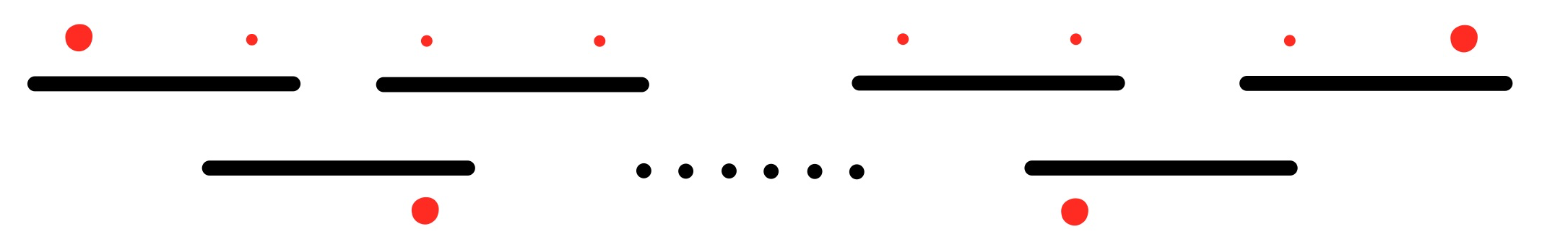
(a) $\mathcal{B}_{\textrm{oe}}$, ‘odd-even’ operators.

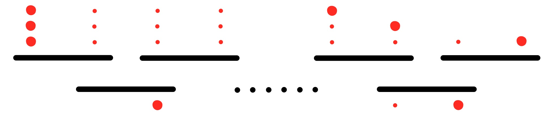
(b) $\mathcal{B}_{\textrm{oo}}$, ‘odd-odd’ operators.

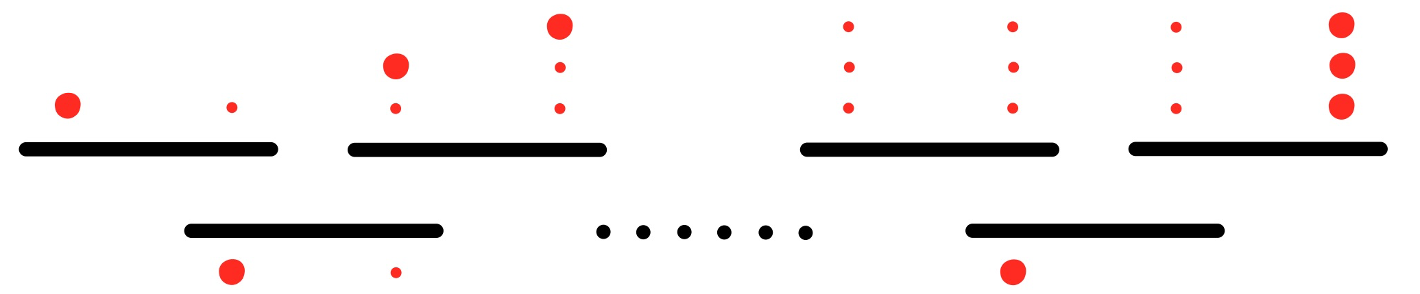
(c) $\mathcal{B}_{\textrm{eo}}$, ‘even-odd’ operators.

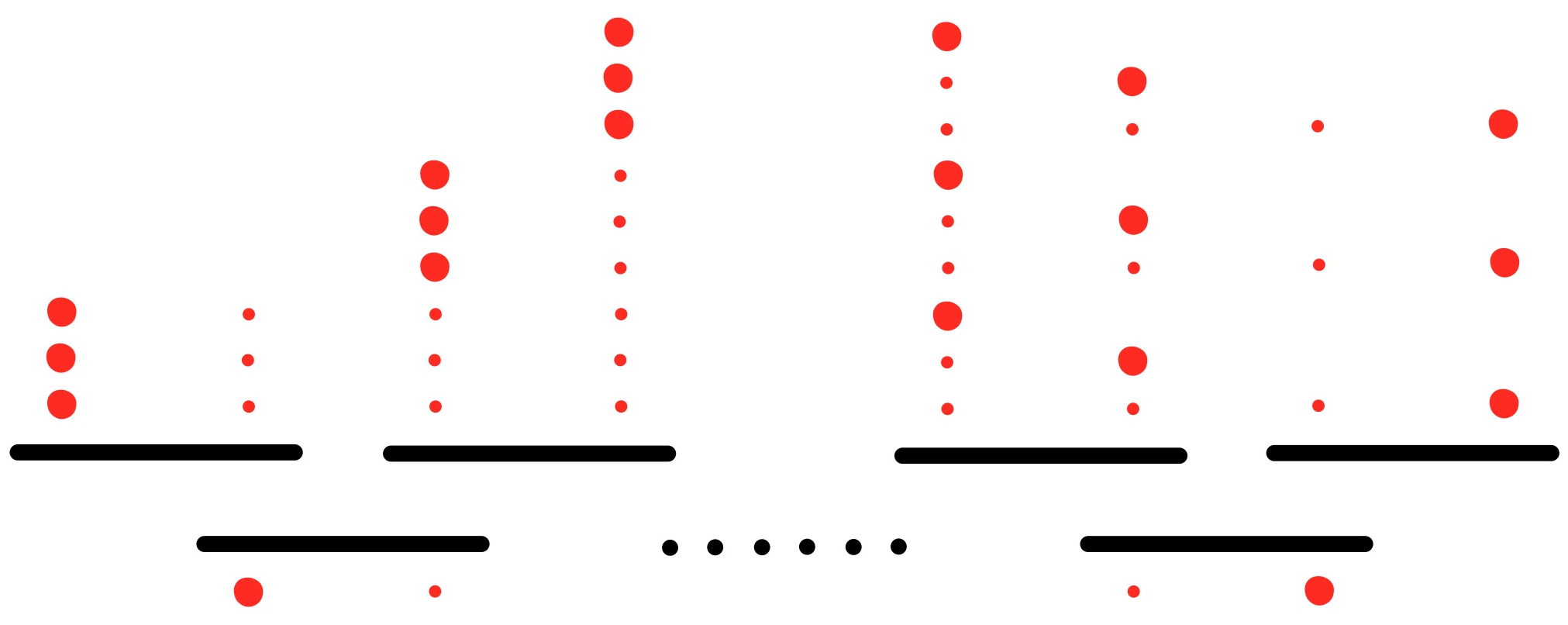
(d) $\mathcal{B}_{\textrm{ee}}$, ‘even-even’ operators.

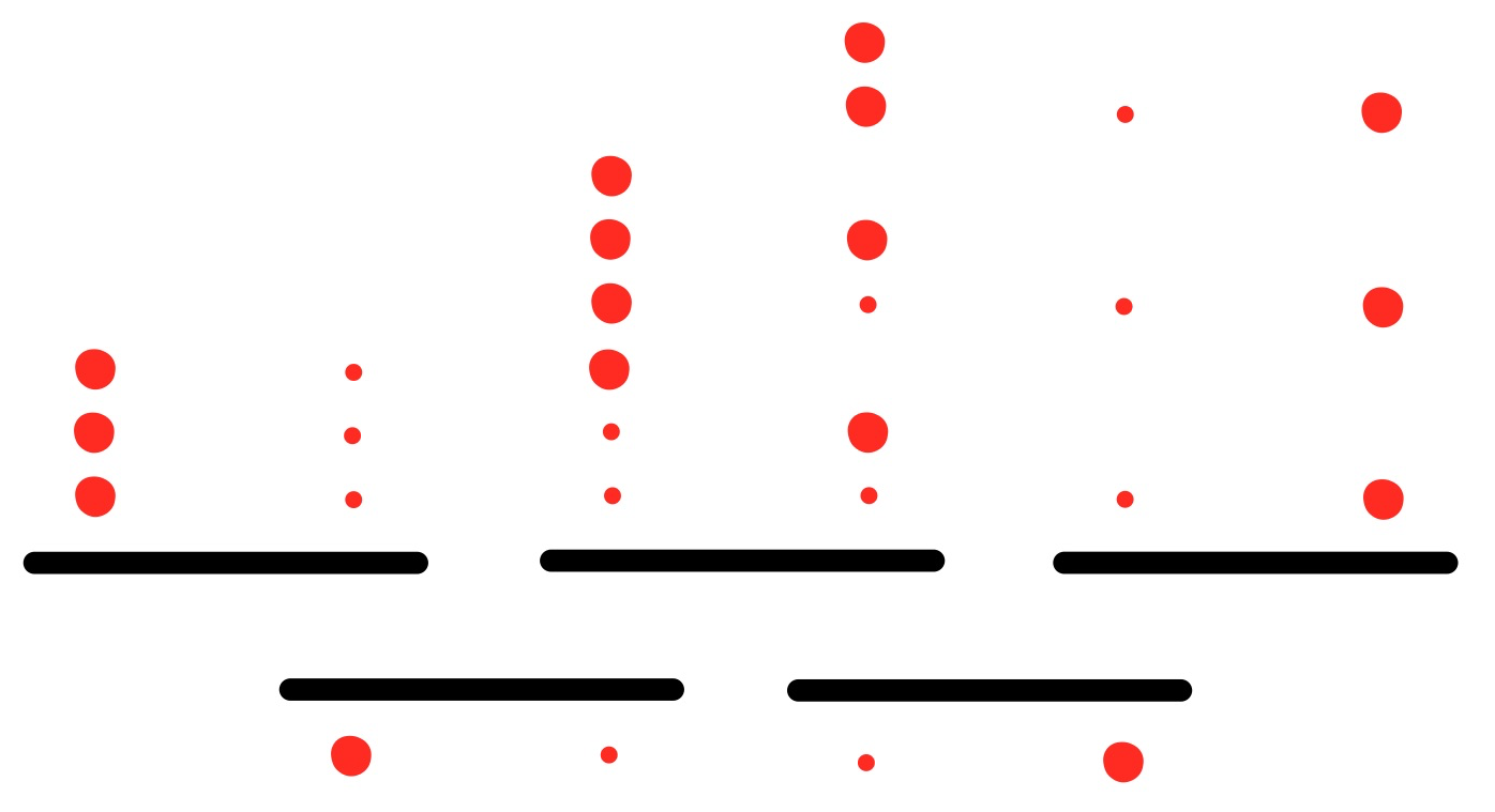
(e) $\mathcal{B}_{\textrm{ee}}$, ‘even-even’ operators with $w=4$.

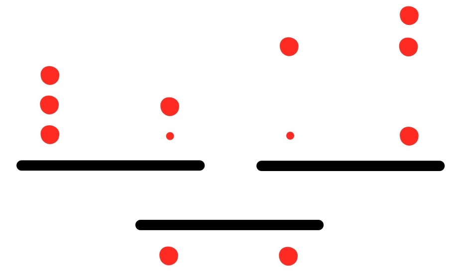
(f) $\mathcal{B}_{\textrm{ee}}$, ‘even-even’ operators with $w=2$.

Figure 2: Diagrams showing how the support of a finite-range operator, supported on a chain of qudits over an interval of $w$ neighbouring sites, can change under conjugation by a dual-unitary Floquet operator $\mathbb{U}$ (as defined in Eqn. 3). The initial operator is shown at the bottom of each diagram, with a site on which it is strictly traceless shown with a large red dot, and a site on which its trace is unspecified (i.e. any value in the interval $[0,d]$) shown with a smaller red dot. Dual-unitary conjugation by $\mathbb{U}$ is then applied, with each gate represented by a horizontal black line (where we are working in the folded picture). The possible operator strings (in terms of the positions of non-trivial support) that the original operator can be mapped in to are shown after (above) the gates. The parity of $x$ (the left-hand most site of non-trivial support) and $w$ turns out to be relevant, due to the restrictions on how the support of an operator can change under dual-unitary dynamics (see Property 1), and so different diagrams are shown for the different possible combinations of these two parities: 2(a)) $\mathcal{B}_{\textrm{oe}}$, $x$-odd, $w$-even; 2(b)) $\mathcal{B}_{\textrm{oo}}$, $x$-odd, $w$-odd; 2(c)) $\mathcal{B}_{\textrm{eo}}$, $x$-even, $w$-odd; 2(d)) $\mathcal{B}_{\textrm{ee}}$, $x$-even, $w$-even; 2(e)) $\mathcal{B}_{\textrm{ee}}$, with $w=4$; 2(f)) $\mathcal{B}_{\textrm{ee}}$, with $w=2$. It is necessary to consider the two edge cases for $\mathcal{B}_{\textrm{ee}}$, as it is possible for terms within $\mathcal{B}_{\textrm{ee}}$ to be mapped back into $\mathcal{B}_{\textrm{ee}}$ by $\mathbb{U}$ but with a decrease in the width by four sites; as the width approaches zero, the possible mappings under $\mathbb{U}$ will be restricted further by the fact that the two ends of the operator are now causally connected. It is not necessary to consider such edge cases with any of the other subspaces, as the endpoints will always remain causally unconnected (under the caveat that $w\leq 2L-4$; throughout this section, a stricter assumption of $w\leq L-4$ is enforced, which ensures this holds).

Figure 3: We collate the results shown in Fig. 2 into a digraph, where the subspaces are nodes of the graph and the transitions between them allowed under conjugation by a dual-unitary Floquet operator are represented by directed edges. The labels on each directed edge denote the width of the terms that can be produced in the subspace associated with the tip of the edge, when starting from a term of width $w$ in the subspace at the base of the edge. We see that the ‘even-$x$, even-$w$’ subspace is a global source - no subspaces can be mapped into it, and all other subspaces can be reached from it - of the digraph, and the ‘odd-$x$, even-$w$’ subspace is a global sink - all subspaces can be mapped into it, and no other subspaces can be reached from it. Looped arrows have been drawn showing the transitions that allow a subspace to be mapped into itself: the red arrows represent transitions where the width must change under these mappings, leading to these transitions being unable to contribute to conserved quantities, as proven in Lemmas 1, 2, and 3; the blue arrows represent transitions where the width of the terms remains the same - it is precisely these transitions which can contribute to solitonic conserved quantities. Note that in constructing this digraph, we must assume that $w\leq L-4$ for all terms before the action of $\mathbb{U}$; this is to ensure that all terms produced after the action of $\mathbb{U}$ have $w\leq L$ (the most any term can grow under the action of $\mathbb{U}$ is $w\mapsto w+4$), such that all terms produced by the action of $\mathbb{U}$ fall into the subspaces $\mathcal{B}_{i},\;i\in\{ee,eo,oe,oo\}$ (which, as defined above, require $w\leq L$). As such, all the Lemmas in this appendix rely on any operators due to be acted upon by $\mathbb{U}$ having $w\leq L-4$.

The mappings between the different $\mathcal{B}$ subspaces under dual-unitary conjugation by $\mathbb{U}$ can be derived by considering the diagrams in Fig. 2, and these mappings are collated into a directed graph in Fig. 3. One of the first things that we can note by studying Fig. 3 is that we cannot have any terms in the subspace $\mathcal{B}_{\textrm{ee}}$ contribute to a quantity $\mathcal{Q}$ if we want $\mathcal{Q}$ to be conserved under the action of a brickwork dual-unitary Floquet operator. We provide a proof of this below.

Lemma 1.

No even-even terms. Let

$$Q=\sum_{x\in\mathbb{Z}_{2L}}\sum_{w\in\mathbb{Z}_{L-3}/0}\bm{q}(x,w)_{x,...,x+w-1}$$ (88)

with $\bm{q}(x,w)\in\bar{\mathcal{A}}_{w}$ be a conserved quantity under the dynamics of a 1+1D brickwork Floquet operator (Eqn. 3), $\mathbb{U}\mathcal{Q}\mathbb{U}^{\dagger}=\mathcal{Q}$. If $\mathbb{U}$ is dual-unitary, then $Q$ cannot contain any terms $\bm{a}\in\mathcal{B}_{\textrm{ee}}$ (i.e. operators with even $x$ and even width $w\leq L-4$),

$$\tr\left(Q^{\dagger}\bm{a}\right)=0\;\;\forall\;\bm{a}\in\mathcal{B}_{\textrm{ee}}.$$ (89)

Proof.

For proof by contradiction, let’s say that $\mathcal{Q}$ does contain some terms from the even-even subspace (i.e. there exists some $\bm{a}\in\mathcal{B}_{\textrm{ee}}$ such that $\tr\left(\mathcal{Q}^{\dagger}\bm{a}\right)\neq 0$) - one of these terms will be the widest such term. Let’s say this term has a width $w_{\textrm{max}}$.

From Fig. 3, we can note that this term will either be mapped by $\mathbb{U}$ into a new term in $\mathcal{B}_{\textrm{ee}}$ with width $w_{\textrm{max}}-4$, or into terms in the other subspaces (if $w_{\textrm{max}}\leq 4$). We can also note that there is no way to map from terms in the other subspace to terms in the even-even subspace.

Putting these two facts together, we can conclude that we won’t have any terms of width $w_{\textrm{max}}$ in the even-even subspace present in $\mathbb{U}\mathcal{Q}\mathbb{U}^{\dagger}$ (recall the elements in the other subspaces will be orthogonal to those in $\mathcal{B}_{\textrm{ee}}$, so we will not be able to reconstruct any even-even terms from terms in the other subspaces) - but this would mean that $\mathcal{Q}\neq\mathbb{U}\mathcal{Q}\mathbb{U}^{\dagger}$, in contradiction with our requirement that $\mathcal{Q}$ is a conserved quantity. We can hence conclude that we cannot have this widest even-even term present in $\mathcal{Q}$ (if we want it to be conserved). But, as we have already stated, if we have any even-even terms present in $\mathcal{Q}$ then we will have one which is the widest. Hence, we must conclude that $\tr\left(Q^{\dagger}\bm{a}\right)=0\;\;\forall\;\bm{a}\in\mathcal{B}_{\textrm{ee}}$ as required.

∎

Next, we can note that terms in the ‘odd-even’ subspace cannot form a conserved quantity by themselves - $\mathcal{Q}$ cannot consist solely of terms with odd $x$ and even $w$.

Lemma 2.

Odd-even terms not sufficient. Let

$$Q=\sum_{x\in\mathbb{Z}_{2L}}\sum_{w\in\mathbb{Z}_{L-3}/0}\bm{q}(x,w)_{x,...,x+w-1}$$ (90)

with $\bm{q}(x,w)\in\bar{\mathcal{A}}_{w}$. If $Q$ consists solely of terms with $x$ odd and $w$ even, then it cannot be a conserved quantity under a brickwork dual-unitary Floquet operator $\mathbb{U}$. Concretely, defining the set

$$A=\{\bm{q}_{x,...,x+w-1}|\tr\left(\mathcal{Q}^{\dagger}\bm{q}_{x,...,x+w-1}\right)\neq 0,\;x\in\mathbb{Z}_{2L},\;w\in\mathbb{Z}_{L-3}/0,\;\bm{q}\in\bar{\mathcal{A}}_{w}\},$$ (91)

then

$$A\subseteq\mathcal{B}_{\textrm{oe}}\implies\mathbb{U}Q\mathbb{U}^{\dagger}\neq Q.$$ (92)

Proof.

Suppose $A\subseteq\mathcal{B}_{\textrm{oe}}$. There will be some $\bm{q}(x,w)_{x,...,x+w-1}\in\mathcal{B}_{\textrm{oe}}$ which contributes to $\mathcal{Q}$ for which $w$ is minimum. Let’s say this term has a width $w_{\textrm{min}}$.

From Fig. 2(a), we can see that all elements of $\mathcal{B}_{\textrm{oe}}$ remain in $\mathcal{B}_{\textrm{oe}}$ (as long as $w\leq L-4$, which is assumed in the statement of the Lemma) and grow in width by 4 sites under the action of a dual-unitary Floquet operator $\mathbb{U}$. Consequently, there will be no terms of width $w_{\textrm{min}}$ present in $\mathbb{U}\mathcal{Q}\mathbb{U}^{\dagger}$. Hence, $\mathcal{Q}\neq\mathbb{U}\mathcal{Q}\mathbb{U}^{\dagger}$. ∎

Finally, we can prove that a quantity that is conserved under the action of a dual-unitary Floquet operator $\mathbb{U}$ can only consist of terms from the subspaces with odd-$w$.

Lemma 3.

Only odd-width terms. Let

$$\mathcal{Q}=\sum_{x\in\mathbb{Z}_{2L}}\sum_{w\in\mathbb{Z}_{L-3}/0}\bm{q}(x,w)_{x,...,x+w-1}$$ (93)

with $\bm{q}(x,w)\in\bar{\mathcal{A}}_{w}$, and let $\mathbb{U}$ be a 1+1D brickwork dual-unitary Floquet operator (Eqn.3). Then

$$\mathbb{U}\mathcal{Q}\mathbb{U}^{\dagger}=\mathcal{Q}\implies\bm{q}(x,w)=0\;\forall\;w\in\mathbb{E}_{L-4}.$$ (94)

Proof.

By Lemma 1, we already know that $\bm{q}(x,w)=0\;\forall\;(x,w)\in\mathbb{E}_{2L}\times\mathbb{E}_{L-4}$. Hence, let us write $\mathcal{Q}$ as

$$\mathcal{Q}=\mathcal{Q}_{odd-w}+\mathcal{Q}_{odd-even},$$ (95)

where

$$\mathcal{Q}_{odd-w}=\sum_{x\in\mathbb{Z}_{2L}}\sum_{w\in\mathbb{O}_{L-4}}\bm{q}(x,w)_{x,...,x+w-1}\in\textrm{Span}\left(\mathcal{B}_{eo}\cup\mathcal{B}_{oo}\right),$$ (96)

and

$$\mathcal{Q}_{odd-even}=\sum_{x\in\mathbb{O}_{2L}}\sum_{w\in\mathbb{E}_{L-4}}\bm{q}(x,w)_{x,...,x+w-1}\in\textrm{Span}\left(\mathcal{B}_{oe}\right),$$ (97)

We know, by the diagrams given in Fig. 2, that under the action of a dual-unitary Floquet operator, $\mathbb{U}$, we can have 3 types of terms produced from these 2 components: we can have terms in the odd-$w$ subspaces which remain in these subspaces - we will denote the new terms with $\mathcal{Q}^{\prime}_{odd-w}$; we can have some terms in $\mathcal{B}_{oe}$ which terms from the odd-$w$ subspaces are mapped into - we will denote these terms with $\mathcal{Q}^{\prime}_{odd-w\mapsto odd-even}$; finally, we will have terms in $\mathcal{B}_{oe}$ which the original $\mathcal{B}_{oe}$ terms (in $\mathcal{Q}_{odd-even}$) are mapped into - we will denote these terms with $\mathcal{Q}^{\prime}_{odd-even}$. Together, this gives

$$\mathbb{U}\mathcal{Q}\mathbb{U}^{\dagger}=\mathcal{Q}^{\prime}_{odd-w}+\mathcal{Q}^{\prime}_{odd-w\mapsto odd-even}+\mathcal{Q}^{\prime}_{odd-even}.$$ (98)

If $\mathcal{Q}$ is to be a conserved quantity, we require that

$$\mathcal{Q}^{\prime}_{odd-w}=\mathcal{Q}_{odd_{w}},$$ (99)

and

$$\mathcal{Q}^{\prime}_{odd-even}+\mathcal{Q}^{\prime}_{odd-w\mapsto odd-even}=\mathcal{Q}_{odd-even},$$ (100)

in order to ensure that $\mathcal{Q}=\mathbb{U}\mathcal{Q}\mathbb{U}^{\dagger}$. If $\mathcal{Q}_{odd-even}\neq 0$, then by Lemma 2 we know that $\mathcal{Q}^{\prime}_{odd-even}\neq\mathcal{Q}_{odd-even}$, and so we require that $\mathcal{Q}^{\prime}_{odd-w\mapsto odd-even}=\mathcal{Q}^{\prime}_{odd-even}-\mathcal{Q}_{odd-even}$ is non-zero such that Eqn. 100 holds. However, if $\mathcal{Q}^{\prime}_{odd-w\mapsto odd-even}\neq 0$ is non-zero, and $\mathcal{Q}^{\prime}_{odd-w}=\mathcal{Q}_{odd_{w}}$, then we will have that the norm of the terms produced by acting on $\mathcal{Q}_{odd-w}$ is greater than the norm of $\mathcal{Q}_{odd-w}$ itself; this contradicts the assumption that $\mathbb{U}$ is unitary - unitary transformations are, by definition, norm-preserving. The only way to resolve this is if $\mathcal{Q}_{odd-even}=0$, in which case

$$\mathcal{Q}=\mathcal{Q}_{odd-w}=\sum_{x\in\mathbb{Z}_{2L}}\sum_{w\in\mathbb{O}_{L-4}}\bm{q}(x,w)_{x,...,x+w-1},$$ (101)

and hence

$$\bm{q}(x,w)=0\;\forall\;w\in\mathbb{E}_{L-4}.$$ (102)

∎

Appendix B The unitary subspaces of the $\mathcal{M}_{\pm,w}$ maps

In the proof of Theorem 1, we use the fact that any operator $\bm{a}\in\bar{\mathcal{A}}_{w}$ supported strictly non-trivially over an interval $[x,x+w-1]$ which is mapped to a new operator supported strictly non-trivially over an interval $[x\pm 2t,x+w-1\pm 2t]$ by $t$ repeated applications of the Floquet operator can be decomposed into a basis of solitons; here, we rigorously establish this fact. Specifically, we show that the subspace spanned by the solitons of the $\mathcal{M}_{\pm,w}$ maps is the same as the subspace spanned by operators which remain the same width and lead to a preservation of norm under repeated applications of the $\mathcal{M}_{\pm,w}$ maps (which is an equivalent statement to that of the previous sentence).

Lemma 4.

Take a dual-unitary Floquet operator, $\mathbb{U}$, as defined in Eqn. 3. Consider the following subspaces of $\bar{\mathcal{A}}_{w}$, defined as

$$\mathcal{S}_{+,w}=\textrm{Span}\left(\bm{a}\in\bar{\mathcal{A}}_{w}\;:\;\mathcal{M}_{+,w}^{t}(\bm{a})\in\bar{\mathcal{A}}_{w},\;\|\mathcal{M}_{+,w}^{t}(\bm{a})\|=\|\bm{a}\|,\;\forall\;t\in\mathbb{N}\right),$$ (103)

and

$$\mathcal{S}_{-,w}=\textrm{Span}\Bigl{(}\bigl{\{}\bm{b}\in\bar{\mathcal{A}}_{w}\;:\;\mathcal{M}_{-,w}^{t}(\bm{b})\in\bar{\mathcal{A}}_{w},\;\|\mathcal{M}_{-,w}^{t}(\bm{b})\|=\|\bm{b}\|,\;\forall\;t\in\mathbb{N}\bigr{\}}\Bigr{)},$$ (104)

where $\|A\|=\sqrt{\tr(A^{\dagger}A)}$ is the Hilbert-Schmidt norm. The right-moving width-$w$ solitons, defined as the elements of the set $\mathbb{S}_{+,w}$ in Eqn. 30, form a complete basis for $\mathcal{S}_{+,w}$, and the left-moving width-$w$ solitons, defined as the elements of the set $\mathbb{S}_{+,w}$ in Eqn. 31, form a complete basis for $\mathcal{S}_{-,w}$. That is,

$$\textrm{Span}\left(\mathbb{S}_{+,w}\right)=\mathcal{S}_{+,w},\quad\textrm{Span}\left(\mathbb{S}_{-,w}\right)=\mathcal{S}_{-,w}.$$ (105)

Proof.

We start by considering the $\mathcal{S}_{+,w}$ subspace, and define a map

$$f:\mathcal{S}_{+,w}\mapsto\mathcal{S}_{+,w},$$ (106)

which is the restriction of $\mathcal{M}_{+,w}$ to $\mathcal{S}_{+,w}$, i.e.

$$f(\bm{a})=\mathcal{M}_{+,w}(\bm{a}).$$ (107)

Trivially, $f$ is linear, and also preserves the Hilbert-Schmidt inner product

$$\langle\bm{a},\bm{c}\rangle =\tr\left(\bm{a}^{\dagger}\bm{c}\right)$$ (108)

$$=\frac{1}{d^{2L-w}}\tr\left(\mathbb{U}^{\dagger}\mathbb{U}\bm{a}^{\dagger}_{\mathcal{R}}\bm{c}_{\mathcal{R}}\right),\quad|\mathcal{R}|=w$$ (109)

$$=\frac{1}{d^{2L-w}}\tr\left(\mathbb{U}\bm{a}^{\dagger}_{\mathcal{R}}\mathbb{U}^{\dagger}\mathbb{U}\bm{c}_{\mathcal{R}}\mathbb{U}^{\dagger}\right)$$ (110)

$$=\frac{1}{d^{2L-w}}\tr\left(\left[\mathcal{M}_{+,w}(\bm{a}^{\dagger})\right]_{\mathcal{R}+2}\left[\mathcal{M}_{+,w}(\bm{c})\right]_{\mathcal{R}+2}\right)$$ (111)

$$=\tr\left(\mathcal{M}_{+,w}(\bm{a})^{\dagger}\mathcal{M}_{+,w}(\bm{c})\right)$$ (112)

$$=\langle f(\bm{a}),f(\bm{c})\rangle,$$ (113)

where we have defined an interval $\mathcal{R}=[x,x+w-1]$ such that $x$ is even, and noted that $\mathcal{M}_{\pm,w}(\bm{a})^{\dagger}=\mathcal{M}_{\pm,w}(\bm{a}^{\dagger})$ and so $f(\bm{a}^{\dagger})=f(\bm{a})^{\dagger}$. We also note that, by definition, $f$ is an endomorphism, $f\in\textrm{End}(\mathcal{S}_{+,w})$. This allows us to deduce that $f$ is a unitary transformation, and hence its eigenvectors must form a complete orthonormal basis for $\mathcal{S}_{+,w}$. For these eigenvectors, which we will conveniently denote as $\{\bm{a_{k}}\}_{k=1}^{n}$, with $1\leq n=(\textrm{dim}(\mathcal{S}_{+,w})-1)\leq d^{2^{w}}-1$, it will be true that

$$\mathbb{U}([\bm{a_{k}}]_{x,...,x+w-1})\mathbb{U}^{\dagger}=\lambda_{k,w}[\bm{a_{k}}]_{x+2,...,x+w+1},\quad\lambda_{k,w}\in\mathbb{C},\;|\lambda_{k,w}|=1,$$ (114)

which makes them all right-moving, width-$w$ solitons - the elements of the set $\mathbb{S}_{+,w}$ defined in Eqn. 30; these eigenvectors are the solitons, and we have shown that they span a unitary subspace $\mathcal{S}_{+,w}$ of the $\mathcal{M}_{+,w}$ map. The proof that the left-moving width-$w$ solitons - the elements of the set $\mathbb{S}_{-,w}$ - span a unitary subspace of the $\mathcal{M}_{-,w}$ map follows completely analogously. We conclude by noting the resemblance this illuminates between the $\mathcal{S}_{\pm,w}$ subspaces and the well-known notion of decoherence-free subspaces [55, 56] (i.e. they are subspaces of $\mathcal{H}_{w}$ on which the generically non-unitary $\mathcal{M}_{\pm,w}$ maps act unitarily). ∎

References

- Nahum et al. [2017] A. Nahum, J. Ruhman, S. Vijay, and J. Haah, Quantum entanglement growth under random unitary dynamics, Phys. Rev. X 7, 031016 (2017).
- Nahum et al. [2018] A. Nahum, S. Vijay, and J. Haah, Operator spreading in random unitary circuits, Phys. Rev. X 8, 021014 (2018).
- von Keyserlingk et al. [2018] C. W. von Keyserlingk, T. Rakovszky, F. Pollmann, and S. L. Sondhi, Operator hydrodynamics, OTOCs, and entanglement growth in systems without conservation laws, Phys. Rev. X 8, 021013 (2018).
- Bertini and Piroli [2020] B. Bertini and L. Piroli, Scrambling in random unitary circuits: Exact results, Phys. Rev. B 102, 064305 (2020).
- Chan et al. [2018] A. Chan, A. De Luca, and J. T. Chalker, Solution of a minimal model for many-body quantum chaos, Phys. Rev. X 8, 041019 (2018).
- Bertini et al. [2019a] B. Bertini, P. Kos, and T. Prosen, Exact correlation functions for dual-unitary lattice models in dimensions, Phys. Rev. Lett. 123, 210601 (2019a).
- Bertini et al. [2021] B. Bertini, P. Kos, and T. Prosen, Random matrix spectral form factor of dual-unitary quantum circuits, Communications in Mathematical Physics 387, 597 (2021).
- Claeys and Lamacraft [2020] P. W. Claeys and A. Lamacraft, Maximum velocity quantum circuits, Phys. Rev. Research 2, 033032 (2020).
- Claeys and Lamacraft [2021] P. W. Claeys and A. Lamacraft, Ergodic and nonergodic dual-unitary quantum circuits with arbitrary local Hilbert space dimension, Phys. Rev. Lett. 126, 100603 (2021).
- Aravinda et al. [2021] S. Aravinda, S. A. Rather, and A. Lakshminarayan, From dual-unitary to quantum Bernoulli circuits: Role of the entangling power in constructing a quantum ergodic hierarchy, Phys. Rev. Research 3, 043034 (2021).
- Rather et al. [2020] S. A. Rather, S. Aravinda, and A. Lakshminarayan, Creating ensembles of dual unitary and maximally entangling quantum evolutions, Phys. Rev. Lett. 125, 070501 (2020).
- Rather et al. [2022] S. A. Rather, S. Aravinda, and A. Lakshminarayan, Construction and local equivalence of dual-unitary operators: From dynamical maps to quantum combinatorial designs, PRX Quantum 3, 040331 (2022).
- Borsi and Pozsgay [2022] M. Borsi and B. Pozsgay, Construction and the ergodicity properties of dual unitary quantum circuits, Phys. Rev. B 106, 014302 (2022).
- Prosen [2021] T. Prosen, Many-body quantum chaos and dual-unitarity round-a-face, Chaos: An Interdisciplinary Journal of Nonlinear Science 31, 093101 (2021), https://pubs.aip.org/aip/cha/article-pdf/doi/10.1063/5.0056970/14634880/093101_1_online.pdf .
- Bertini et al. [2019b] B. Bertini, P. Kos, and T. Prosen, Entanglement spreading in a minimal model of maximal many-body quantum chaos, Phys. Rev. X 9, 021033 (2019b).
- Gopalakrishnan and Lamacraft [2019] S. Gopalakrishnan and A. Lamacraft, Unitary circuits of finite depth and infinite width from quantum channels, Phys. Rev. B 100, 064309 (2019).
- Piroli et al. [2020] L. Piroli, B. Bertini, J. I. Cirac, and T. Prosen, Exact dynamics in dual-unitary quantum circuits, Phys. Rev. B 101, 094304 (2020).
- Reid and Bertini [2021] I. Reid and B. Bertini, Entanglement barriers in dual-unitary circuits, Phys. Rev. B 104, 014301 (2021).
- Zhou and Harrow [2022] T. Zhou and A. W. Harrow, Maximal entanglement velocity implies dual unitarity, Phys. Rev. B 106, L201104 (2022).
- Foligno and Bertini [2023] A. Foligno and B. Bertini, Growth of entanglement of generic states under dual-unitary dynamics, Phys. Rev. B 107, 174311 (2023).
- Bertini et al. [2020a] B. Bertini, P. Kos, and T. Prosen, Operator entanglement in local quantum circuits I: Chaotic dual-unitary circuits, SciPost Phys. 8, 067 (2020a).
- Bertini et al. [2020b] B. Bertini, P. Kos, and T. Prosen, Operator entanglement in local quantum circuits II: Solitons in chains of qubits, SciPost Phys. 8, 068 (2020b).
- Fritzsch and Prosen [2021] F. Fritzsch and T. Prosen, Eigenstate thermalization in dual-unitary quantum circuits: Asymptotics of spectral functions, Phys. Rev. E 103, 062133 (2021).
- Ippoliti and Ho [2023] M. Ippoliti and W. W. Ho, Dynamical purification and the emergence of quantum state designs from the projected ensemble, PRX Quantum 4, 030322 (2023).
- Ho and Choi [2022] W. W. Ho and S. Choi, Exact emergent quantum state designs from quantum chaotic dynamics, Phys. Rev. Lett. 128, 060601 (2022).
- Claeys and Lamacraft [2022] P. W. Claeys and A. Lamacraft, Emergent quantum state designs and biunitarity in dual-unitary circuit dynamics, Quantum 6, 738 (2022).
- Rampp and Claeys [2023] M. A. Rampp and P. W. Claeys, Hayden-Preskill recovery in chaotic and integrable unitary circuit dynamics (2023), arXiv:2312.03838 [quant-ph] .
- Zhou and Nahum [2020] T. Zhou and A. Nahum, Entanglement membrane in chaotic many-body systems, Phys. Rev. X 10, 031066 (2020).
- Ippoliti et al. [2022] M. Ippoliti, T. Rakovszky, and V. Khemani, Fractal, logarithmic, and volume-law entangled nonthermal steady states via spacetime duality, Phys. Rev. X 12, 011045 (2022).
- Ippoliti and Khemani [2021] M. Ippoliti and V. Khemani, Postselection-free entanglement dynamics via spacetime duality, Phys. Rev. Lett. 126, 060501 (2021).
- Lu and Grover [2021] T.-C. Lu and T. Grover, Spacetime duality between localization transitions and measurement-induced transitions, PRX Quantum 2, 040319 (2021).
- Claeys et al. [2022] P. W. Claeys, M. Henry, J. Vicary, and A. Lamacraft, Exact dynamics in dual-unitary quantum circuits with projective measurements, Phys. Rev. Res. 4, 043212 (2022).
- Kos and Styliaris [2023] P. Kos and G. Styliaris, Circuits of space and time quantum channels, Quantum 7, 1020 (2023).
- Masanes [2023] Ll. Masanes, Discrete holography in dual-unitary circuits (2023), arXiv:2301.02825 [hep-th] .
- Suzuki et al. [2022] R. Suzuki, K. Mitarai, and K. Fujii, Computational power of one- and two-dimensional dual-unitary quantum circuits, Quantum 6, 631 (2022).
- Logarić et al. [2023] L. Logarić, S. Dooley, S. Pappalardi, and J. Goold, Quantum many-body scars in dual unitary circuits (2023), arXiv:2307.06755 [quant-ph] .
- Stephen et al. [2022] D. T. Stephen, W. W. Ho, T.-C. Wei, R. Raussendorf, and R. Verresen, Universal measurement-based quantum computation in a one-dimensional architecture enabled by dual-unitary circuits (2022), arXiv:2209.06191 [quant-ph] .
- Kos et al. [2021] P. Kos, B. Bertini, and T. Prosen, Correlations in perturbed dual-unitary circuits: Efficient path-integral formula, Phys. Rev. X 11, 011022 (2021).
- Rampp et al. [2023a] M. A. Rampp, R. Moessner, and P. W. Claeys, From dual unitarity to generic quantum operator spreading, Phys. Rev. Lett. 130, 130402 (2023a).
- Yu et al. [2023] X.-H. Yu, Z. Wang, and P. Kos, Hierarchical generalization of dual unitarity (2023), arXiv:2307.03138 [quant-ph] .
- Foligno et al. [2023] A. Foligno, P. Kos, and B. Bertini, Quantum information spreading in generalised dual-unitary circuits (2023), arXiv:2312.02940 [cond-mat.stat-mech] .
- Liu and Ho [2023] C. Liu and W. W. Ho, Solvable entanglement dynamics in quantum circuits with generalized dual unitarity (2023), arXiv:2312.12239 [quant-ph] .
- Rampp et al. [2023b] M. A. Rampp, S. A. Rather, and P. W. Claeys, The entanglement membrane in exactly solvable lattice models (2023b), arXiv:2312.12509 [quant-ph] .
- Khemani et al. [2018] V. Khemani, A. Vishwanath, and D. A. Huse, Operator spreading and the emergence of dissipative hydrodynamics under unitary evolution with conservation laws, Phys. Rev. X 8, 031057 (2018).
- Rakovszky et al. [2018] T. Rakovszky, F. Pollmann, and C. W. von Keyserlingk, Diffusive hydrodynamics of out-of-time-ordered correlators with charge conservation, Phys. Rev. X 8, 031058 (2018).
- Faddeev and Takhtajan [1987] L. D. Faddeev and L. A. Takhtajan, Hamiltonian methods in the theory of solitons, Classics in Mathematics (Springer, 1987).
- Faddeev [1996] L. D. Faddeev, How Algebraic Bethe Ansatz works for integrable model (1996), arXiv:hep-th/9605187 [hep-th] .
- Gütschow et al. [2010] J. Gütschow, S. Uphoff, R. F. Werner, and Z. Zimborás, Time asymptotics and entanglement generation of Clifford quantum cellular automata, Journal of Mathematical Physics 51, 015203 (2010), https://pubs.aip.org/aip/jmp/article-pdf/doi/10.1063/1.3278513/15961826/015203_1_online.pdf .
- Prosen [2023] T. Prosen, On two non-ergodic reversible cellular automata, one classical, the other quantum, Entropy 25, 10.3390/e25050739 (2023).
- Cervera-Lierta [2018] A. Cervera-Lierta, Exact Ising model simulation on a quantum computer, Quantum 2, 114 (2018).
- Cade et al. [2020] C. Cade, L. Mineh, A. Montanaro, and S. Stanisic, Strategies for solving the Fermi-Hubbard model on near-term quantum computers, Phys. Rev. B 102, 235122 (2020).
- Moudgalya et al. [2022] S. Moudgalya, B. A. Bernevig, and N. Regnault, Quantum many-body scars and Hilbert space fragmentation: a review of exact results, Reports on Progress in Physics 85, 086501 (2022).
- Moudgalya and Motrunich [2022] S. Moudgalya and O. I. Motrunich, Hilbert space fragmentation and commutant algebras, Phys. Rev. X 12, 011050 (2022).
- Li et al. [2023] Y. Li, P. Sala, and F. Pollmann, Hilbert space fragmentation in open quantum systems, Phys. Rev. Res. 5, 043239 (2023).
- Lidar et al. [1998] D. A. Lidar, I. L. Chuang, and K. B. Whaley, Decoherence-free subspaces for quantum computation, Phys. Rev. Lett. 81, 2594 (1998).
- Lidar [2014] D. A. Lidar, Review of decoherence-free subspaces, noiseless subsystems, and dynamical decoupling, in Quantum Information and Computation for Chemistry (John Wiley & Sons, Ltd, 2014) pp. 295–354, https://onlinelibrary.wiley.com/doi/pdf/10.1002/9781118742631.ch11 .
- Bernard and Doyon [2016] D. Bernard and B. Doyon, Conformal field theory out of equilibrium: a review, Journal of Statistical Mechanics: Theory and Experiment 2016, 064005 (2016).
- Cho et al. [2017] G. Y. Cho, K. Shiozaki, S. Ryu, and A. W. W. Ludwig, Relationship between symmetry protected topological phases and boundary conformal field theories via the entanglement spectrum, Journal of Physics A: Mathematical and Theoretical 50, 304002 (2017).
- Po et al. [2016] H. C. Po, L. Fidkowski, T. Morimoto, A. C. Potter, and A. Vishwanath, Chiral Floquet phases of many-body localized bosons, Phys. Rev. X 6, 041070 (2016).
- Po et al. [2017] H. C. Po, L. Fidkowski, A. Vishwanath, and A. C. Potter, Radical chiral Floquet phases in a periodically driven Kitaev model and beyond, Phys. Rev. B 96, 245116 (2017).
- Verresen et al. [2017] R. Verresen, R. Moessner, and F. Pollmann, One-dimensional symmetry protected topological phases and their transitions, Phys. Rev. B 96, 165124 (2017).
- Pérez-García et al. [2008] D. Pérez-García, M. M. Wolf, M. Sanz, F. Verstraete, and J. I. Cirac, String order and symmetries in quantum spin lattices, Phys. Rev. Lett. 100, 167202 (2008).
- Milbradt et al. [2023] R. M. Milbradt, L. Scheller, C. Aßmus, and C. B. Mendl, Ternary unitary quantum lattice models and circuits in dimensions, Phys. Rev. Lett. 130, 090601 (2023).
- Jonay et al. [2021] C. Jonay, V. Khemani, and M. Ippoliti, Triunitary quantum circuits, Phys. Rev. Research 3, 043046 (2021).
- Sommers et al. [2023] G. M. Sommers, D. A. Huse, and M. J. Gullans, Crystalline quantum circuits, PRX Quantum 4, 030313 (2023).
- Haah et al. [2023] J. Haah, L. Fidkowski, and M. B. Hastings, Nontrivial quantum cellular automata in higher dimensions, Communications in Mathematical Physics 398, 469 (2023).
- Haah [2021] J. Haah, Clifford quantum cellular automata: Trivial group in 2D and Witt group in 3D, Journal of Mathematical Physics 62, 092202 (2021), https://pubs.aip.org/aip/jmp/article-pdf/doi/10.1063/5.0022185/16015852/092202_1_online.pdf .
- Freedman and Hastings [2020] M. Freedman and M. B. Hastings, Classification of quantum cellular automata, Communications in Mathematical Physics 376, 1171 (2020).
- Freedman et al. [2022] M. Freedman, J. Haah, and M. B. Hastings, The group structure of quantum cellular automata, Communications in Mathematical Physics 389, 1277 (2022).
- Shirley et al. [2022] W. Shirley, Y.-A. Chen, A. Dua, T. D. Ellison, N. Tantivasadakarn, and D. J. Williamson, Three-dimensional quantum cellular automata from chiral semion surface topological order and beyond, PRX Quantum 3, 030326 (2022).
- Stephen et al. [2019] D. T. Stephen, H. P. Nautrup, J. Bermejo-Vega, J. Eisert, and R. Raussendorf, Subsystem symmetries, quantum cellular automata, and computational phases of quantum matter, Quantum 3, 142 (2019).