Two-loop mixed QCD-electroweak amplitudes for $Z+$jet production at the LHC: bosonic corrections

Abstract

We present a calculation of the bosonic contribution to the two-loop mixed QCD-electroweak scattering amplitudes for $Z$-boson production in association with one hard jet at hadron colliders. We employ a method to calculate amplitudes in the ’t Hooft-Veltman scheme that reduces the amount of spurious non-physical information needed at intermediate stages of the computation, to keep the complexity of the calculation under control. We compute all the relevant Feynman integrals numerically using the Auxiliary Mass Flow method. We evaluate the two-loop scattering amplitudes on a two-dimensional grid in the rapidity and transverse momentum of the $Z$ boson, which has been designed to yield a reliable numerical sampling of the boosted-$Z$ region. This result provides an important building block for improving the theoretical modelling of a key background for monojet searches at the LHC.

1 Introduction

The production of a $Z$ boson in association with hadronic jets is a key standard candle at the Large Hadron Collider (LHC). Thanks to its large production rate and its relatively clean dilepton plus jet final state, it allows for a multitude of investigations like detector calibration and luminosity monitoring, validation of Parton Shower Monte Carlo tools, extraction of fundamental Standard Model (SM) parameters, as well as high-precision scrutiny of the structure of the SM and searches for new physics.

Despite the fact that the bulk of the $Z$+jet cross section at the LHC comes from a region where the jet’s transverse momentum is not very large, $p_{\textrm{T},j}\lesssim 100~{}{\rm GeV}$, the number of events where the $Z$ boson is accompanied by a highly-energetic jet is still quite sizable. This allows for very precise measurements all the way up to the TeV scale. Indeed, existing experimental analyses ATLAS:2022nrp ; CMS:2022ilp already have a total uncertainty of just a few percent in the $p_{\textrm{T}}\sim 200~{}{\rm GeV}$ region and around 10% in the highly-boosted $p_{\textrm{T}}\sim 1~{}{\rm TeV}$ region. With ever more data being recorded and analysed, the situation is only going to improve: at the High-Luminosity LHC, few-percent experimental precision is expected up to transverse momenta of the order of 1 TeV, and $\mathcal{O}(10\%)$ precision up to 2.5 TeV Lindert:2017olm .

A good control of $Z$ production in the boosted region allows for interesting physics explorations. For example, precise data in the dilepton channel can constrain otherwise elusive dimension-8 Standard Model Effective Theory (SMEFT) operators Boughezal:2022nof , provided that adequate theoretical predictions are also available. Also, boosted $Z$-boson production in the $Z$ to invisible channel provides a key background for monojet searches at the LHC, where one looks for a high-$p_{\textrm{T}}$ jet recoiling against missing energy ATLAS:2021kxv ; CMS:2021far . Such a signature is very interesting because it is quite common in many new physics models, ranging from weakly coupled dark-matter, to leptoquarks models, supersymmetric scenarios, or large extra dimensions.

In the recent past, there has been a large community-wide effort to improve the theoretical description of boosted vector-boson production. In particular, in ref. Lindert:2017olm the authors provided theoretical predictions that include state-of-the-art NNLO QCD results Gehrmann-DeRidder:2015wbt ; Gehrmann-DeRidder:2016cdi ; Gehrmann-DeRidder:2016jns ; Boughezal:2015ded ; Boughezal:2016isb ; Boughezal:2015dva ; Boughezal:2016dtm ; Campbell:2016lzl ; Campbell:2017dqk and NLO electroweak (EWK) ones Denner:2011vu ; Denner:2012ts ; Kallweit:2015dum ; Denner:2009gj . In the boosted region, the latter are crucial. Indeed, despite being suppressed by the weak coupling constant $\alpha$, they are enhanced by large Sudakov logarithms of the form $\frac{\alpha}{4\pi s_{w}^{2}}\log^{2}(\frac{s}{m_{V}^{2}})$, where $s_{w}$ is the sine of the weak mixing angle, $s$ is a large scale of the process and $m_{V}$ is the vector boson mass, see e.g. Kuhn:1999de . At large scales, EWK corrections then become as large as QCD ones. For this reason, ref. Lindert:2017olm also included the dominant two-loop electroweak effects coming from Sudakov logarithms Kuhn:2005gv ; Kuhn:2005az ; Kuhn:2007qc ; Kuhn:2007cv .

Given the size of QCD and EWK corrections, it is also mandatory to properly control mixed QCD-EWK ones. At present, $\mathcal{O}(\alpha_{s}\alpha)$ corrections to dilepton+jet production are not known. In ref. Lindert:2017olm , the size of these corrections was estimated by essentially multiplying NLO QCD and NLO EWK ones. This prescription is very reasonable at asymptotically-high scales, since Sudakov logarithms and QCD corrections mostly factorise. However, at large but finite energies this approximation is bound to receive corrections. A more rigorous assessment of mixed QCD-EWK corrections then becomes important. In fact, the lack of exact $\mathcal{O}(\alpha_{s}\alpha)$ corrections is now a major bottleneck towards highest-precision theoretical predictions in the boosted region Lindert:2017olm .

Computing $\mathcal{O}(\alpha_{s}\alpha)$ corrections to dilepton+jet or missing-energy+jet production at the LHC poses significant challenges. First, such processes involve a non-trivial mixed QCD-EWK radiation pattern, which requires proper regularisation. Achieving this is complicated if one wants to retain differential information on the final state. This problem has only recently been solved, and only for the simplest processes Behring:2020cqi ; Buccioni:2020cfi ; Dittmaier:2020vra ; Buonocore:2021rxx ; Bonciani:2021zzf ; Buccioni:2022kgy . Although the techniques used for the calculation Buccioni:2022kgy could be extended to deal with more complex processes, this remains a non-trivial task. Second, mixed QCD-EWK corrections for dilepton+jet or missing-energy+jet production require non-trivial two-loop scattering amplitudes. These involve both a complex final state and massive internal virtual particles, which makes the calculation notoriously difficult.

In this article, we perform a first important step towards the calculation of mixed QCD-EWK two-loop scattering amplitudes relevant for boosted dilepton+jet production. To make the problem manageable, we focus on the production of an on-shell $Z$ boson rather than on the production of the dilepton final state, with the idea that this is going to provide the dominant contribution for all observables which are dominated by the $Z$-pole region (and in particular for the observables relevant for the boosted region). This allows us to only consider amplitudes for $2\to 2$ scattering rather than the much more complicated ones relevant for the $2\to 3$ process. Also, we only target the boosted region, where vector-boson resonance effects are not present and hence use of the complex-mass scheme Denner:1999gp ; Denner:2005fg ; Beneke:2004km ; Hoang:2004tg ; Beneke:1997zp for EWK corrections becomes less critical. Finally, as a first non-trivial step towards the full result here we only consider bosonic corrections, i.e. we systematically neglect closed fermion loop corrections. This allows us to set up a framework for computing mixed QCD-EWK corrections without the additional complication of corrections involving top-quark virtual effects, which cannot a-priori be neglected in the boosted region. We believe that our framework could be extended to cover this case as well, but this warrants an investigation on its own. Even in this somewhat simplified setup, an analytical calculation of the amplitude remains challenging. Because of this, we decided to adopt a semi-numerical approach. Our main result is then an evaluation of the two-loop amplitudes over a two-dimensional grid that parametrises the $2\to 2$ kinematics. The grid is designed to provide an adequate coverage of the boosted region.

The remainder of this paper is organised as follows. In sec. 2 we provide details of our notation and of the kinematics of the process. In sec. 3 we describe some methods used in our work i.e. the Lorentz tensor structure of our scattering amplitude in sec. 3.1, and its relation to the leptonic current at fixed helicity in sec. 3.2. In sec. 3.3 we describe our calculation of the bare amplitudes. In sec. 4 we discuss the ultraviolet and infrared structure of our result and we also define one- and two-loop finite remainders. The latter are the main result of our paper. In sec. 5 we document the checks that we have performed on our calculation and illustrate our results. Finally, we conclude in sec. 6. Our results for the finite remainders are available in a computer-readable format in the ancillary material that accompanies this submission.

2 Notation and kinematics

We consider virtual $\mathcal{O}(\alpha\alpha_{s})$ corrections to the production of the $Z$ boson in association with one hadronic jet. We focus on bosonic corrections, i.e. we neglect contributions stemming from closed fermion loops. We then consider the channels

$$q+\bar{q}\to g+Z,~{}~{}~{}~{}~{}q+g\to q+Z,$$ (1)

where $q$ is either an up- or a down-type (anti) quark. We take the CKM matrix to be diagonal, and neglect $b$-quark induced contributions. This way, no virtual top-quark contributions are present.

All the processes in eq. 1 can be obtained by crossing the following master amplitude

$$q(p_{1})+\bar{q}(p_{2})+g(p_{3})+Z(p_{4})\to 0\,,$$ (2)

where $q$ is either an up or a down quark. In this symmetric notation, momentum conservation reads

$$p_{1}+p_{2}+p_{3}+p_{4}=0\,.$$ (3)

All external particles are on-shell

$$p_{1}^{2}=p_{2}^{2}=p_{3}^{2}=0\,,\quad p_{4}^{2}=m_{Z}^{2}\,.$$ (4)

The three kinematic Mandelstam invariants of this process

$$s_{12}=(p_{1}+p_{2})^{2}\,,~{}s_{13}=(p_{1}+p_{3})^{2}\,,~{}s_{23}=(p_{2}+p_{3})^{2}\,,$$ (5)

are related by the momentum-conservation relation

$$s_{12}+s_{13}+s_{23}=m_{Z}^{2}\,.$$ (6)

For physical kinematics, one Mandelstam invariant is positive and two are negative. Results in the Euclidean region where $m_{Z}^{2}<0$ and $s_{ij}<0$ can be analytically continued to the physical Riemann sheet by giving a small positive imaginary part to all the invariants, see ref. Gehrmann:2002zr for a thorough discussion.

For definiteness, we now focus on the $s_{12}>0$, $s_{13},s_{23}<0$ channel. In the partonic center-of-mass frame, the kinematics can be parametrised as follows

$$\begin{split}&p_{1}=\frac{\sqrt{s_{12}}}{2}(1,0,0,1)\,,\\ &p_{2}=\frac{\sqrt{s_{12}}}{2}(1,0,0,-1)\,,\\ &p_{3,\rm phys}=-p_{3}=p_{t,3}\left(\cosh(y_{3}),\cos\phi,\sin\phi,\sinh(y_{3})\right)\,\\ &p_{4,\rm phys}=-p_{4}=\left(m_{t,Z}\cosh(y_{Z}),-p_{t,Z}\cos\phi,-p_{t,Z}\sin\phi,m_{t,Z}\sinh(y_{Z})\right),\end{split}$$ (7)

where $\phi$ is an irrelevant azimuthal angle and $m_{t,Z}=\sqrt{p_{t,Z}^{2}+m_{Z}^{2}}$. The transverse momenta and rapidities of the final-state particles are given in terms of Mandelstam invariants as

$$p_{t,3}=p_{t,Z}=\sqrt{\frac{s_{13}s_{23}}{s_{12}}}\,,~{}~{}~{}y_{3}=\frac{1}{2}\ln\left(\frac{s_{23}}{s_{13}}\right),~{}~{}~{}y_{Z}=\frac{1}{2}\ln\left(\frac{s_{12}+s_{23}}{s_{12}+s_{13}}\right),$$ (8)

with

$$|y_{Z}|\leq\frac{1}{2}\ln\left(\frac{s_{\rm had}+m_{Z}^{2}+\sqrt{(s_{\rm had}-m_{Z}^{2})^{2}-4p_{t,Z}^{2}\,s_{\rm had}}}{s_{\rm had}+m_{Z}^{2}-\sqrt{(s_{\rm had}-m_{Z}^{2})^{2}-4p_{t,Z}^{2}\,s_{\rm had}}}\right),$$ (9)

where $s_{\rm had}$ is the collider center-of-mass energy squared. In what follows, we will either use $\{s_{13},s_{23}\}$ or $\{p_{t,Z},y_{Z}\}$ as independent variables.

To deal with the ultraviolet (UV) and infrared (IR) divergences of the amplitude, we work in dimensional regularisation and set $d=4-2\epsilon$. In particular, we adopt the ’t Hooft-Veltman scheme THOOFT1972189 , i.e. we treat all external particles as purely four-dimensional and the internal ones as $d=(4-2\epsilon)$-dimensional. We write the unrenormalised amplitude as

$$\begin{split}\mathcal{A}_{b}&=T^{a_{3}}_{i_{2}i_{1}}\sqrt{\frac{\alpha_{s,b}}{2\pi}}\sqrt{\frac{\alpha_{b}}{2\pi}}A_{b}(d;\{m_{i,b}\},\{s_{ij}\})\\ &=T^{a_{3}}_{i_{2}i_{1}}\sqrt{\frac{\alpha_{s,b}}{2\pi}}\sqrt{\frac{\alpha_{b}}{2\pi}}\,\epsilon_{3,\mu}(p_{3})\epsilon_{4,\nu}(p_{4})\,\bar{u}(p_{2})A_{b}^{\mu\nu}(d;\{m_{i,b}\},\{s_{ij}\})u(p_{1})\,,\end{split}$$ (10)

where $i_{1}$, $i_{2}$, and $a_{3}$ are colour indices of the quark, antiquark, and gluon, respectively, $\epsilon_{3,\mu}$ and $\epsilon_{4,\nu}$ are the polarization vectors of the massless gluon and of the massive $Z$ boson, $m_{i,b}$, $i\in\{Z,W\}$ are the (bare) vector boson masses, and $\alpha_{b}$, $\alpha_{s,b}$ are the bare electromagnetic and strong couplings, respectively. The dependence on other electroweak parameters like the quark isospin or electric charge is implicitly assumed. Finally, $T^{a}_{ij}$ is the $SU(3)$ generator in the fundamental representation, rescaled such that

$${\rm Tr}[T^{a}T^{b}]=\delta^{ab}.$$ (11)

We find it convenient to express our results in terms of the quadratic Casimir invariants $C_{A}$ and $C_{F}$, which for $SU(N_{c})$ read

$$C_{A}=N_{c}\,,~{}~{}~{}~{}~{}C_{F}=\frac{N_{c}^{2}-1}{2N_{c}}\,.$$ (12)

In QCD, $C_{A}=3$ and $C_{F}=4/3$. The amplitude in eq. 10 can be written as a double perturbative series in the strong and electromagnetic couplings

$$A_{b}=A^{(0,0)}_{b}+\frac{\alpha_{s,b}\,\mu_{0}^{2\epsilon}}{2\pi}\,A^{(1,0)}_{b}+\frac{\alpha_{b}\,\mu_{0}^{2\epsilon}}{2\pi}\,A^{(0,1)}_{b}+\frac{\alpha_{s,b}\,\mu_{0}^{2\epsilon}}{2\pi}\frac{\alpha_{b}\,\mu_{0}^{2\epsilon}}{2\pi}\,A^{(1,1)}_{b}+\mathcal{O}(\alpha_{s,b}^{2},\alpha_{b}^{2})\,,$$ (13)

where we have made explicit the dependence on the dimensionful reference scale $\mu_{0}$ but have kept the dependence of $A_{b}$ and $A_{b}^{(i,j)}$ on the vector boson masses and on the external kinematics implicit.

To obtain the renormalised amplitude $\mathcal{A}$, we multiply $\mathcal{A}_{b}$ by the external wave-function renormalisation factors and express the generic bare parameter $g_{i,b}$ in terms of its renormalised counterpart $g_{i}$. Schematically,

$$\mathcal{A}=\sqrt{Z_{q}Z_{\bar{q}}Z_{g}Z_{Z}}\times\mathcal{A}_{b}\big{|}_{g_{i,b}\to g_{i}}.$$ (14)

We discuss the renormalisation procedure in more detail in sec. 4. Here we only note that we renormalise the strong coupling in the $\overline{\rm MS}$ scheme, and all the EWK parameters in the on-shell scheme. Also, we adopt the $G_{\mu}$ input parameter scheme, i.e. we choose $\{G_{\mu},m_{Z},m_{W}\}$ as independent parameters. For our results, we use $G_{\mu}=1.16639\times 10^{-5}$ ParticleDataGroup:2022pth . Similarly to eq. 10, we write the renormalised amplitude as

$$\begin{split}\mathcal{A}&=T^{a_{3}}_{i_{2}i_{1}}\sqrt{\frac{\alpha_{s}}{2\pi}}\sqrt{\frac{\alpha}{2\pi}}A(d;\{m_{i}\},\{s_{ij}\})\\ &=T^{a_{3}}_{i_{2}i_{1}}\sqrt{\frac{\alpha_{s}}{2\pi}}\sqrt{\frac{\alpha}{2\pi}}\,\epsilon_{3,\mu}(p_{3})\epsilon_{4,\nu}(p_{4})\,\bar{u}(p_{2})A^{\mu\nu}(d;\{m_{i}\},\{s_{ij}\})u(p_{1})\,,\end{split}$$ (15)

and expand $A$ as

$$A=A^{(0,0)}+\frac{\alpha_{s}}{2\pi}\,A^{(1,0)}+\frac{\alpha}{2\pi}\,A^{(0,1)}+\frac{\alpha_{s}}{2\pi}\frac{\alpha}{2\pi}\,A^{(1,1)}+\mathcal{O}(\alpha_{s}^{2},\alpha^{2})\,.$$ (16)

In these equations, $m_{i}$ are the renormalised masses, $\alpha$ is the renormalised electromagnetic coupling and $\alpha_{s}=\alpha_{s}(\mu_{R})$ is the renormalised strong coupling with $\mu_{R}$ the renormalisation scale. The main result of this article is the computation of $A^{(1,1)}$.

3 Details of the calculation

For further convenience, we provide here some details on the formalisms used for our calculation.

3.1 Tensor decomposition

In full generality, the bare scattering amplitudes in eq. 10 can be written as

$$A_{b}^{(l,m)}=\sum_{k=1}^{n_{t}}\overline{\mathcal{F}}^{(l,m)}_{k;b}(d;\{m_{i,b}\},\{s_{ij}\})\,\times\,\overline{T}_{k}\,,$$ (17)

where $\overline{\mathcal{F}}^{(l,m)}_{k;b}$ are scalar form factors and $\overline{T}_{k}=\bar{v}(p_{2})\,\Gamma_{k}^{\mu\nu}\,u(p_{1})\times\epsilon_{3,\mu}(p_{3})\,\epsilon_{4,\nu}(p_{4})$, where $\Gamma_{k}^{\mu\nu}$ are $n_{t}$ independent Lorentz tensors. We now discuss a basis choice for these tensors. First, we note that in this paper we do not consider corrections coming from closed fermion loops. As a consequence, there are no anomalous diagrams and we can take $\gamma_{5}$ as anticommuting. Because of this, it is enough to study the tensor structure of a vector current, and the axial case will follow. For a vector current, by simple enumeration one finds $n_{t}=39$ independent $\Gamma^{\mu\nu}_{i}$ structures. Using the Dirac equation for the external on-shell quarks $\bar{v}_{2}\,\not{p}_{2}=\not{p}_{1}u_{1}=0$, as well as the transversality condition for the massless gluon $\epsilon_{3}\cdot p_{3}=0$, $n_{t}$ decreases by 26. Finally, if one also uses the $Z$-boson transversality condition $\epsilon_{4}\cdot p_{4}$ and fixes the reference momentum $q_{3}$ for the polarisation vector $\epsilon_{3}$ to the momentum of one of the external fermions, one is left with $n_{t}=7$ independent $d$-dimensional tensor structures.

Following ref. Gehrmann:2022vuk , we set $q_{3}=p_{2}$, such that

$$\epsilon_{3}\cdot p_{2}=0\,,$$ (18)

and define the first six tensors as follows

$$\Gamma_{1}^{\mu\nu} =p_{1}^{\nu}\gamma^{\mu}\,,\;\;\;\;\;\Gamma_{2}^{\mu\nu}=p_{1}^{\mu}p_{1}^{\nu}\not{p}_{3}\,,$$

$$\Gamma_{3}^{\mu\nu} =p_{2}^{\nu}\gamma^{\mu}\,,\;\;\;\;\;\Gamma_{4}^{\mu\nu}=p_{1}^{\mu}\gamma^{\nu}\,,$$

$$\Gamma_{5}^{\mu\nu} =p_{1}^{\mu}p_{2}^{\nu}\not{p}_{3}\,,\;\;\Gamma_{6}^{\mu\nu}=g^{\mu\nu}\not{p}_{3}\,.$$ (19)

These six structures span the the whole space of purely four-dimensional tensors Peraro:2019cjj ; Peraro:2020sfm . We can then construct the last structure to only have components in the unphysical $(-2\epsilon)$-dimensional space. This can be done through a simple orthogonalisation procedure Peraro:2019cjj ; Peraro:2020sfm , which yields

$$\overline{T}_{7}\,\,=\bar{v}(p_{2})\not{\epsilon}_{3}\not{p}_{3}\not{\epsilon}_{4}u(p_{1})-\frac{1}{s}\left(s(\overline{T}_{3}+\overline{T}_{6}-\overline{T}_{1})+t\overline{T}_{t}+u(\overline{T}_{1}+\overline{T}_{4})-2\overline{T}_{5}\right).$$ (20)

Since in strict $d$ dimensions the seven tensors are independent, there cannot be any cancellation of IR and UV singularities among the different $\overline{T}_{i}$. Hence, the renormalised and IR-regulated form factor $\overline{\mathcal{F}}_{7}^{(i,j)}$ cannot have any poles. Since the corresponding tensor $\overline{T}_{7}$ is evanescent by construction, the contribution of $\overline{\mathcal{F}}_{7}^{(i,j)}$ drops from the final result if one works in the ’t Hooft-Veltman scheme and sets $d=4$ after the renormalisation and IR-regularisation procedure. Therefore, in the ’t Hooft-Veltman scheme, all physical results can be obtained from the first six tensor structures alone Peraro:2019cjj ; Peraro:2020sfm . We note that the number of independent tensors coincides with the number of independent helicity states of the external particles, i.e. it matches the independent four-dimensional degrees of freedom. A relation between the six tensor structures in eq. 19 and the independent helicity amplitudes is discussed in the next sub-section.

Since the six tensors in eq. (19) span the physical space, it is always possible to find coefficients $c_{ik}$ such that

$$\sum_{\rm pol}\mathcal{P}_{i}\,\overline{T}_{j}\equiv\sum_{\rm pol}\left(\sum_{k=1}^{n_{t}}c_{ik}\overline{T}_{k}^{\dagger}\right)\overline{T}_{j}=\delta_{ij}.$$ (21)

In fact, solving these equations for $c_{ik}$ is a matter of trivial algebra. For convenience, we report them in appendix A. The projector operators $\mathcal{P}_{i}$ defined in eq. 21 can then be used to extract the $\overline{\mathcal{F}}_{k;b}^{(i,j)}$ form factor from the bare amplitude

$$\overline{\mathcal{F}}^{(i,j)}_{k;b}=\sum_{\rm pol}\mathcal{P}_{k}A_{b}\,.$$ (22)

Finally, we stress that the tensors 19 have been determined under the transversality condition $p_{i}\cdot\epsilon_{i}=0$ and with the reference momentum choice $q_{3}=p_{2}$. It is then important to use the following expressions for the sum over polarisations of the external gluon and gauge boson

$$\begin{split}\sum_{\rm pol}\epsilon_{3}^{*\mu}\epsilon_{3}^{\nu}&=-g^{\mu\nu}+\frac{p_{2}^{\mu}p_{3}^{\nu}+p_{3}^{\mu}p_{2}^{\nu}}{p_{2}\cdot p_{3}}\,,\\ \sum_{\rm pol}\epsilon_{4}^{*\mu}\epsilon_{4}^{\nu}&=-g^{\mu\nu}+\frac{p_{4}^{\mu}p_{4}^{\nu}}{m_{Z}^{2}}\,.\end{split}$$ (23)

We close this section by discussing how to generalise the above construction to the case of different left- and right-handed interactions. As we already mentioned, if we neglect closed fermion loops there are no anomalous diagrams and one can treat $\gamma_{5}$ as anticommuting. This makes such generalisation straightforward. The amplitude eq. 17 can be decomposed as

$$A_{b}^{(l,m)}=\sum_{c=L,R}\sum_{k=1}^{n_{t}}\overline{\mathcal{F}}^{(l,m)}_{k,c;b}(d;\{m_{i,b}\},\{s_{ij}\})\,\times\,\overline{T}_{k,c}\,,$$ (24)

with

$$\overline{T}_{i,L/R}=\bar{v}(p_{2})\,\Gamma_{i}^{\mu\nu}\left(\frac{1\mp\gamma_{5}}{2}\right)\,u(p_{1})\times\epsilon_{3,\mu}(p_{3})\,\epsilon_{4,\nu}(p_{4}),$$ (25)

and $\Gamma^{\mu\nu}_{i}$ defined in eq. 19. Projectors onto the left/right form factors $\overline{\mathcal{F}}^{(l,m)}_{i,b,L/R}$ can be performed using the same procedure explained above, see eqs 21, 22, with the replacements $\overline{T}^{(\dagger)}_{i}\to\overline{T}^{(\dagger)}_{i,L/R}$, and $c_{ik}\to c_{ik}/2$. In practice, we always work with vector-current tensors and projectors, and then dress them with relevant left- and right-handed couplings. This allows us to effectively halve the various tensor manipulations on the amplitude.

3.2 Helicity amplitudes

The form factors $\overline{\mathcal{F}}_{i}$ introduced in the previous section can be used to obtain the helicity amplitudes for the process

$$q(p_{1})+\bar{q}(p_{2})+g(p_{3})+\bar{l}(p_{5})+l(p_{6})\to 0,$$ (26)

where $l$ and $\bar{l}$ are a pair of massless leptons. In the pole approximation Stuart:1991xk ; Aeppli:1993rs and neglecting $\mathcal{O}(\alpha^{2})$ corrections, the amplitude can be schematically written as

$$A=i\sum_{\lambda_{Z}}\frac{\mathcal{M}^{\rm prod}(\lambda_{Z})\times\mathcal{M}^{\rm dec}(\lambda_{Z})}{p_{Z}^{2}-m_{Z}^{2}+im_{Z}\Gamma_{Z}}+{\rm non~{}resonant},$$ (27)

where “prod”/“dec” refers to the amplitude for the production/decay of an on-shell $Z$ boson ($p_{Z}^{2}=m_{Z}^{2}$) with polarisation $\lambda_{Z}$. The numerator in eq. 27 can be written in terms of the tensor structures introduced in sec. 3.1 as

$$\begin{split}\mathcal{M}\equiv&\sum_{\lambda_{Z}}\mathcal{M}^{\rm prod}(\lambda_{Z})\times\mathcal{M}^{\rm dec}(\lambda_{Z})=\\ &\sum_{k}\bar{v}(p_{2})\Gamma_{k}^{\alpha\mu}\left[\overline{\mathcal{F}}_{k,L}\left(\frac{1-\gamma_{5}}{2}\right)+\overline{\mathcal{F}}_{k,R}\left(\frac{1+\gamma_{5}}{2}\right)\right]u(p_{1})\,\epsilon_{\alpha}(p_{3})\times\\ &\left[-g^{\mu\nu}+\frac{p_{Z}^{\mu}p_{Z}^{\nu}}{m_{Z}^{2}}\right]\times\bar{v}(p_{5})\gamma_{\nu}\left[c_{l,L}\left(\frac{1-\gamma_{5}}{2}\right)+c_{l,R}\left(\frac{1+\gamma_{5}}{2}\right)\right]u(p_{6})\,,\end{split}$$ (28)

with $p_{Z}=p_{5}+p_{6}=-p_{1}-p_{2}-p_{3}$, and $p_{Z}^{2}=m_{Z}^{2}$. In eq. 28, $c_{l,L}$, $c_{l,R}$ are generalised left- and right-handed couplings that parameterise the $Zl\bar{l}$ vertex. At LO, they are given by

$$c^{\rm LO}_{l,L}=ie\times\frac{I^{3}_{l}-s_{w}^{2}Q_{l}}{s_{w}c_{w}},~{}~{}~{}c^{\rm LO}_{l,R}=-ie\times\frac{s_{w}Q_{l}}{c_{w}},$$ (29)

where $I^{3}_{l}=\pm 1/2$ is the weak isospin of the lepton $l$, $Q_{l}$ is its electric charge in units of $e$ ($Q_{e}=-1$ for an electron), and $s_{w}=\sin\theta_{w}$, $c_{w}=\cos\theta_{w}$ with $\theta_{w}$ the weak mixing angle. For mixed QCD-EWK corrections, one needs $c_{l,R/L}$ up to $\mathcal{O}(\alpha\alpha_{s})$. These are well known, see e.g. refs Dittmaier:2009cr ; Dittmaier:2015rxo , so we won’t discuss them further.

The amplitude $\mathcal{M}$ in eq. 28 can be easily projected to helicity states. To do so, we use the spinor-helicity formalism (see e.g. Dixon:1996wi ) and write left- and right-handed currents as

$$\bar{v}(p_{2})\gamma^{\mu}\left(\frac{1-\gamma_{5}}{2}\right)u(p_{1})=\langle 2\gamma^{\mu}1],~{}~{}~{}~{}\bar{v}(p_{2})\gamma^{\mu}\left(\frac{1+\gamma_{5}}{2}\right)u(p_{1})=[2\gamma^{\mu}1\rangle.$$ (30)

We also define the helicity of a particle/antiparticle to be equal/opposite to its chirality, and write the polarisation vector of the incoming gluon as

$$\epsilon^{\mu}_{+}(p_{3})=-\frac{1}{\sqrt{2}}\frac{[q_{3}\gamma^{\mu}3\rangle}{[q_{3}3]},~{}~{}~{}\epsilon^{\mu}_{-}(p_{3})=\frac{1}{\sqrt{2}}\frac{\langle q_{3}\gamma^{\mu}3]}{\langle q_{3}3\rangle},$$ (31)

with $q_{3}$ the reference momentum the gluon, $q_{3}\cdot\epsilon_{3}=p_{3}\cdot\epsilon_{3}=0$. We remind the reader that our tensor $\overline{T}_{i}$ have been constructed using the choice $q_{3}=p_{2}$. With these assignments, the helicity amplitudes $\mathcal{M}_{\vec{\lambda}}$, $\vec{\lambda}=\{\lambda_{1},\lambda_{2},\lambda_{3},\lambda_{5},\lambda_{6}\}$ for the all-incoming process eq. 26 read

$$\begin{split}\mathcal{M}_{-+-+-}&=\,\,\,\,\,\frac{c_{l,L}}{\sqrt{2}}\left(\langle 12\rangle[13]^{2}\left(\alpha_{1,L}\langle 536]+\alpha_{2,L}\langle 526]\right)+\alpha_{3,L}\langle 25\rangle[13][36]\right),\\ \mathcal{M}_{-+++-}&=\,\,\,\,\,\frac{c_{l,L}}{\sqrt{2}}\left(\langle 23\rangle^{2}[12]\left(\gamma_{1,L}\langle 536]+\gamma_{2,L}\langle 516]\right)+\gamma_{3,L}\langle 23\rangle\langle 35\rangle[16]\right),\\ \mathcal{M}_{+--+-}&=-\frac{c_{l,L}}{\sqrt{2}}\left([23]^{2}\langle 12\rangle\left(\gamma_{1,R}\langle 536]+\gamma_{2,R}\langle 516]\right)+\gamma_{3,R}[23][36]\langle 15\rangle\right),\\ \mathcal{M}_{+-++-}&=-\frac{c_{l,L}}{\sqrt{2}}\left([12]\langle 13\rangle^{2}\left(\alpha_{1,R}\langle 536]+\alpha_{2,R}\langle 526]\right)+\alpha_{3,R}[26]\langle 13\rangle\langle 35\rangle\right),\end{split}$$ (32)

with

$$\begin{split}\alpha_{1,i}&=-\overline{\mathcal{F}}_{2,i}\,,\qquad\alpha_{2,i}=\overline{\mathcal{F}}_{5,i}-\overline{\mathcal{F}}_{2,i}+\frac{2}{s_{23}}\overline{\mathcal{F}}_{4,i}\,,\qquad\alpha_{3,i}=2\overline{\mathcal{F}}_{6,i}-\frac{2s_{12}}{s_{23}}\overline{\mathcal{F}}_{4,i}\,,\\ \gamma_{1,i}&=\frac{1}{s_{23}}\left(s_{13}\overline{\mathcal{F}}_{5,i}+2(\overline{\mathcal{F}}_{3,i}-\overline{\mathcal{F}}_{6,i})\right)\,,\\ \gamma_{2,i}&=\frac{1}{s_{23}}\left(s_{13}(\overline{\mathcal{F}}_{5,i}-\overline{\mathcal{F}}_{2,i})-2(\overline{\mathcal{F}}_{1,i}-\overline{\mathcal{F}}_{3,i}+\overline{\mathcal{F}}_{4,i})\right)\,,\\ \gamma_{3,i}&=-\frac{2}{s_{23}}\left(s_{23}\overline{\mathcal{F}}_{6,i}+s_{12}\overline{\mathcal{F}}_{4,i}\right)\,,\end{split}$$ (33)

and $i=L,R$. The amplitudes with $\{\lambda_{5},\lambda_{6}\}=\{-,+\}$ can obtained from the expressions 32 for $\{\lambda_{5},\lambda_{6}\}=\{-,+\}$ through the replacements $|5\rangle\to|5]$, $|6]\to|6\rangle$, $c_{l,L}\to c_{l,R}$. Using these results, it is straightforward to reconstruct any amplitude from the $\overline{\mathcal{F}}$ form factors. Because of this, we will focus on the latter in what follows. We conclude this section by pointing out that eq. 32 is in agreement with eqns (5.6-5.17) of ref. Gehrmann:2022vuk once all the small differences in notation are accounted for.

3.3 Computation of the bare amplitude

Figure 1: Example Feynman diagrams corresponding to top integral topologies.

	${A}_{b}^{(0,0)}$	${A}_{b}^{(1,0)}$	${A}_{b}^{(0,1)}$	${A}_{b}^{(1,1)}$
# non-vanishing diagrams	2	11	27	462
# integral topologies	0	1	4	18
# scalar integrals	0	105	275	60968

Table 1: Complexity comparison at different loop orders.

We now describe the calculation of the bare two-loop mixed QCD-EWK factors $\overline{\mathcal{F}}$. We start with generating, using Qgraf Nogueira:1991ex , all the relevant Feynman diagrams contributing to the bare amplitude $A_{b}^{(1,1)}$, see fig. 1 for few representatives. As we already mentioned, we neglect closed fermion loops and bottom-induced contributions. We are left with 462 non-vanishing Feynman diagrams $(\text{FD})^{(1,1)}_{f}$,

$${A}_{b}^{(1,1)}=\sum_{f=1}^{462}(\text{FD})^{(1,1)}_{f}\,.$$ (34)

Comparing to lower orders, (see tab. 1) the complexity grows significantly, thus making the efficiency of the calculation crucial. For this reason, we first perform a useful parallelisation criterion, and only later the projection of the amplitude onto the tensor structures introduced in sec. 3.1. To this end, we split the Feynman diagrams by their graph structure.

In the two-loop four-point amplitude, each Feynman diagram can have at most 7 virtual propagators. We will refer to diagrams containing a set of 7 different virtual propagators as top sector diagrams. Given the kinematics of the problem, there are 9 independent Lorentz invariants involving loop momenta $k_{i}$, $i=1,2$. Out of these, 3 are of the type $k_{i}\cdot k_{j}$ and 6 of the type $p_{i}\cdot k_{j}$. These 9 invariants can be linearly related to the 7 top sector propagators complemented with 2 additional irreducible scalar products (ISPs), which for convenience we also choose to be of the propagator type. We will refer to this set of 9 propagators as an integral topology. One can find a minimal set of integral topologies onto which all Feynman diagrams can be mapped. For our case, we require 18 basic topologies, as well as their 61 crossings. We report the definition of the 18 basic topologies in appendix B, and in computer-readable format in an ancillary file provided with this submission. Feynman diagrams with a smaller number of virtual propagators can be obtained by pinching top sector diagrams, which often makes their mapping onto an integral topology not unique. In practice, we perform this mapping by finding an appropriate loop momenta shift with Reduze 2 vonManteuffel:2012np ; Studerus:2009ye . As a result, we split the whole set of Feynman diagrams contributing to $\mathcal{A}_{b}^{(1,1)}$ by integral topology type $t$

$${A}_{b}^{(1,1)}=\sum_{t\in\text{topo}}{A}^{(1,1)}_{b,t}\,.$$ (35)

Common structures of different integral topologies are typically revealed only after loop-momenta integration and/or expansion in $\epsilon$. Hence, grouping Feynman diagrams by topology and performing preliminary manipulations separately for each topology provides an efficient parallelisation strategy.

To actually compute the amplitude, we work in the Feynman gauge. After substituting the Feynman rules, we immediately perform the colour algebra and write our result in terms of $C_{A}$ and $C_{F}$, see eq. 12. Next, we project on the 12 form factors $\overline{\mathcal{F}}_{1,...,6,L/R;b}$ defined in sec. 3.1. To do so, we apply the $\mathcal{P}_{i}$ projectors (see sec. 3.1) and evaluate all required traces of Dirac gamma matrices in $d$-dimensions with Form Vermaseren:2000nd , treating $\gamma_{5}$ as anticommuting. At the end, each form factor can be written as

$$\overline{\mathcal{F}}^{(1,1)}_{i,L/R;b}=\sum_{t}\sum_{f\,\in\,\text{FD}_{t}}\int\frac{d^{d}k_{1}}{(2\pi)^{d}}\frac{d^{d}k_{2}}{(2\pi)^{d}}\,\frac{\mathcal{N}_{i,L/R,f}(d;\{m_{i}\},\{p_{i}\cdot p_{j}\},\{p_{i}\cdot k_{j}\},\{k_{i}\cdot k_{j}\})}{\mathcal{D}_{t,1}^{n_{f,1}}\dots\mathcal{D}_{t,7}^{n_{f,7}}}\,,$$ (36)

where the first sum runs over all the relevant topologies, FD_t is the set of Feynman diagrams mapped onto a given topology $t$, $\mathcal{N}$ is a polynomial in the space-time dimension $d$, the $Z$ and $W$ masses and scalar products involving both loop and external momenta, $\mathcal{D}_{t,i}$ is the $i$-th denominator factor of the topology $t$ (see appendix B for their explicit definition), and $n_{f,i}\in\{0,1,2\}$. For convenience, we linearly relate all the 9 independent kinematic invariants involving loop momenta, which are present in numerators $\mathcal{N}$, to the complete set of propagators $\vec{\mathcal{D}}_{t}$, fixed by the integral topology $t$, such that eq. 36 assumes the form

$$\overline{\mathcal{F}}^{(1,1)}_{i,L/R;b}=\sum_{t}\sum_{\vec{n}\,\in\,\text{int set}}\widetilde{\mathcal{N}}_{i,t,\vec{n}}(d;m_{i},\{p_{i}\cdot p_{j}\})\,\mathcal{I}_{t,\vec{n}}\,,\qquad n_{i}\in[-4,2]\cap\mathbb{Z}\,,$$ (37)

with now

$$\mathcal{I}_{t,\vec{n}}\equiv\int\frac{d^{d}k_{1}}{(2\pi)^{d}}\frac{d^{d}k_{2}}{(2\pi)^{d}}\,\frac{1}{\mathcal{D}_{t,1}^{n_{1}}\cdots\mathcal{D}_{t,9}^{n_{9}}}\,.$$ (38)

It is well-known that the $\mathcal{I}_{t,\vec{n}}$ integrals are not independent. Indeed, they satisfy so-called Integration-By-Parts (IBP) identities Chetyrkin:1981qh . Typically, only after the form factors are expressed in terms of a minimal set of independent master integrals (MIs) one sees a significant reduction in the complexity of the $\widetilde{\mathcal{N}}$ coefficients, as redundancies tend to be minimised.

Since in our problem there are many mass scales, satisfactorily performing a fully-analytic reduction of the amplitude in terms of MIs is complicated. In particular, the step of expressing the various integrals in terms of MIs typically introduces complex rational functions. Although these are expected to greatly simplify when all the pieces of the amplitude are combined together, achieving such a simplification is non-trivial. Fortunately, we can simplify our calculation by setting the $W$ and $Z$ masses to numerical values. For numerical efficiency, we choose the $m_{W}^{2}/m_{Z}^{2}$ ratio to be a simple rational number, while being close enough to its actual value. In particular, we choose

$$\begin{split}m_{Z}&=91.1876\;\mathrm{GeV}\,,\\ m_{W}&=\sqrt{\frac{7}{9}}m_{Z}=80.4199\;\mathrm{GeV}\,.\end{split}$$ (39)

Such a choice for the $W$ mass differ from its actual value by few permille, and it is fully adequate for our phenomenological purposes. Setting the $Z$ and $W$ mass to numbers vastly reduces the parametric complexity of the integral structure. Keeping both the dimensional-regularisation parameter $\epsilon$ and the kinematics invariant $\{s_{13},s_{23}\}$ symbolic, we generate IBP identities by LiteRed Lee:2012cn ; Lee:2013mka and solve them by the finite field arithmetic vonManteuffel:2014ixa ; Peraro:2016wsq implemented in FiniteFlow Peraro:2019svx . We also employ the method described in ref. Liu:2023cgs to exploit linear relations among the reduction coefficients, which can effectively utilize their common structures to reduce the number of finite-field samples. Comparing to the traditional reconstruction strategy, this method can improve the computational efficiency by approximately an order of magnitude in our computation.

After reducing the amplitude to MIs, we evaluate the latter using the power-expansion-based differential equations method Kotikov:1990kg ; Czakon:2008zk . To this end, we construct a differential equation for master integrals with respect to the kinematics invariants $s_{13}$ and $s_{23}$. Schematically,

$$\partial_{x}\vec{I} =\mathbf{A}_{x}(\epsilon,s_{13},s_{23})\vec{I},\quad\quad x\in\{s_{13},s_{23}\}$$ (40)

where $\vec{I}$ is a vector containing all the MIs and ${\mathbf{A}}_{x}$, are matrices. Such a writing is possible since the MIs provide a basis not only for integrals but also for all their possible derivatives. To solve the differential equations, we first compute the boundary conditions by numerically evaluating the MIs at the following regular point in $s_{12}$ scattering region:

$$\frac{s_{13}}{m_{Z}^{2}}=-\frac{31}{11},\quad\frac{s_{23}}{m_{Z}^{2}}=-\frac{13}{7}.$$ (41)

To do this, we use AMFlow Liu:2022chg which implements the auxiliary mass flow method Liu:2017jxz ; Bronnum-Hansen:2020mzk ; Liu:2021wks , which has already proven very successful in many complex calculations, see e.g. Chen:2022vzo ; Chen:2022mre ; FebresCordero:2023gjh . With differential equations and boundary conditions in hand, the master integrals have already been fully determined. What we need to do in practice is just to use the differential equations solver in AMFlow to solve them from the boundary point to any desired phase space points. We compute the $\epsilon$ expansion of our results by fitting 10 numerical samples obtained using specific numerical values for $\epsilon$ Liu:2022chg . To make sure that we retain enough numerical precision even in case of large cancellations among terms, at this stage we evaluate all the MIs with about 120-digit precision. From these 10 numerical samples, we reconstruct the $\epsilon$ expansion of the result directly at the level of the form factors, without first reconstructing the analogous expansion for the MIs. After this procedure, we expect our leading pole to have very high precision of about 50 digits or better. We then lose a bit of precision for each subsequent order in $\epsilon$, but still we estimate that our final part retains about 20-digit precision or better.

In this way, we are able to numerically evaluate all the $\overline{\mathcal{F}}$ form factors at a given phase-space point in a robust and relatively efficient way. Contrary to a fully-analytic result, such an evaluation cannot be kinematically crossed. Therefore, we need in principle to provide 6 separate results for the independent channels $u\,\bar{u}\to g\,Z$, $u\,g\to u\,Z$, $g\,u\to u\,Z$, $d\,\bar{d}\to g\,Z$, $d\,g\to d\,Z$, $g\,d\to d\,Z$. In practice, we evaluate our result on a two-dimensional $\{p_{t,Z},y_{Z}\}$ grid that is symmetric under $p_{1}\leftrightarrow p_{2}$ exchange, see sec. 5. As a consequence, we only need to compute results for the four channels $u\,\bar{u}\to g\,Z$, $u\,g\to u\,Z$, $d\,\bar{d}\to g\,Z$, $d\,g\to d\,Z$.

4 UV renormalisation and IR regularisation

The bare two-loop mixed QCD-EWK amplitude ${A}^{(1,1)}_{b}$ has pole singularities in $\epsilon$ starting at $\epsilon^{-4}$, stemming from UV and IR divergences. As we mentioned in sec. 2, we renormalise the strong coupling in the $\overline{\rm MS}$ scheme, all the EWK parameters in the on-shell scheme, and we adopt the $G_{\mu}$ input-parameter scheme. To renormalise our result, one has to write the bare parameters in terms of the renormalised ones and to multiply by the relevant $Z$-factors, see eq. 14. To be more concrete, we expand our bare form factors as

$$\begin{split}\overline{\mathcal{F}}_{i,c;b}=\sqrt{\frac{\alpha_{s,b}}{2\pi}}\sqrt{\frac{\alpha_{b}}{2\pi}}\bigg{[}\overline{\mathcal{F}}^{(0,0)}_{i,c;b}+\frac{\alpha_{s,b}\,\mu_{0}^{2\epsilon}}{2\pi}\,\overline{\mathcal{F}}^{(1,0)}_{i,c;b}+\frac{\alpha_{b}\,\mu_{0}^{2\epsilon}}{2\pi}\,\overline{\mathcal{F}}^{(0,1)}_{i,c;b}+\\ \frac{\alpha_{s,b}\,\mu_{0}^{2\epsilon}}{2\pi}\frac{\alpha_{b}\,\mu_{0}^{2\epsilon}}{2\pi}\,\overline{\mathcal{F}}^{(1,1)}_{i,c;b}+\mathcal{O}(\alpha_{s,b}^{2},\alpha_{b}^{2})\bigg{]}\,,\end{split}$$ (42)

with $i=1,...,6$ and $c=L,R$, see eq. 13. We also define renormalised form factors through the expansion

$$\begin{split}\overline{\mathcal{F}}_{i,c}=\sqrt{\frac{\alpha_{s}}{2\pi}}\sqrt{\frac{\alpha}{2\pi}}\bigg{[}\overline{\mathcal{F}}^{(0,0)}_{i,c}+\frac{\alpha_{s}}{2\pi}\,\overline{\mathcal{F}}^{(1,0)}_{i,c}+\frac{\alpha}{2\pi}\,\overline{\mathcal{F}}^{(0,1)}_{i,c}+\frac{\alpha_{s}}{2\pi}\frac{\alpha}{2\pi}\,\overline{\mathcal{F}}^{(1,1)}_{i,c}+\mathcal{O}(\alpha_{s}^{2},\alpha^{2})\bigg{]}\,,\end{split}$$ (43)

with now $\alpha_{s}=\alpha_{s}(\mu)$. Similarly to eq. 14, bare and renormalised form factors are schematically related by

$$\overline{\mathcal{F}}_{i,c}=\sqrt{Z_{q,c}Z_{\bar{q},c}Z_{g}Z_{Z}}\times\mathcal{\overline{\mathcal{F}}}_{b,c}\big{|}_{g_{i,b}\to g_{i}}.$$ (44)

At $\mathcal{O}(\alpha_{s})$, all the $Z_{i}$ factors are equal to one and the QCD renormalisation procedure amounts to writing the bare coupling $\alpha_{s,b}$ in terms of the $\overline{\rm MS}$ one as

$$S_{\epsilon}\mu_{0}^{2\epsilon}\alpha_{s,b}=\mu^{2\epsilon}\alpha_{s}\left[1-\frac{\beta_{0}}{\epsilon}\left(\frac{\alpha_{s}}{2\pi}\right)+\mathcal{O}(\alpha_{s}^{2})\right],$$ (45)

with $S_{\epsilon}=(4\pi)^{\epsilon}e^{-\gamma_{E}\epsilon}$ and $\alpha_{s}=\alpha_{s}(\mu)$. If we neglect contributions coming from closed fermion loops, $\beta_{0}$ reads

$$\beta_{0}=\frac{11}{6}C_{A}.$$ (46)

The $\mathcal{O}(\alpha)$ EWK renormalisation procedure is more complicated. However, since at this order neither the strong coupling nor $Z_{g}$ receive corrections, it is formally identical to the renormalisation of the $q\bar{q}Z$ vertex. To this order, we can write

$$\overline{\mathcal{F}}_{i,c}=\left[1+\frac{\alpha}{2\pi}\delta_{{\rm UV},c}^{(0,1)}\right]\overline{\mathcal{F}}_{i,c;b},$$ (47)

with Dittmaier:2009cr

$$\delta_{{\rm UV},c}^{(0,1)}=\frac{1}{2}\left(2\delta_{Z_{q,c}}+\delta_{Z_{ZZ}}-\frac{Q_{q}}{g_{q,c}}\delta_{Z_{\gamma Z}}\right)+\frac{\delta_{g_{q,c}}}{g_{q,c}}.$$ (48)

In this equation,

$$g_{q,L}=\frac{I^{3}_{q}-s_{w}^{2}Q_{q}}{s_{w}c_{w}}\,,\quad\quad g_{q,R}=-\frac{s_{w}Q_{q}}{c_{w}}\,,$$ (49)

where $Q$ is the electric charge of the external quark in units of $e$ ($Q_{up}=\frac{2}{3}$, $Q_{dn}=-\frac{1}{3}$), $I^{3}_{q}$ is the third component of its weak isospin ($I^{3}_{up}=\frac{1}{2}$,$I^{3}_{dn}=-\frac{1}{2}$), $c_{w}=\frac{m_{W}}{m_{Z}}$ and $s_{w}=\sqrt{1-c_{w}^{2}}$. Note the $\gamma Z$ kinetic mixing term $\delta_{Z_{\gamma Z}}$ in eq. 48, which can be accounted for by a simple refactoring of the overall coupling. Note also that, contrarily to the $\overline{\rm MS}$ renormalization scheme, in the on-shell scheme, the counterterms have a non-trivial $\epsilon$ expansion. Their explicit expression up to $\mathcal{O}(\epsilon^{0})$ can be found e.g. in ref. Denner:1991kt .

At $\mathcal{O}(\alpha\alpha_{s})$, there is a non-trivial interplay between QCD and EWK renormalisation. However, the situation drastically simplifies if one neglects contributions coming from closed fermion loops. Indeed, in this case still $Z_{g}=1$. Also, the QCD and EWK renormalisation procedures almost decouple from each other. Precisely, only the quark wave-function renormalisation factor $Z_{q}$ receives $\mathcal{O}(\alpha\alpha_{s})$ contributions. For left-handed quarks, it reads Buccioni:2020cfi ; Behring:2020cqi

$$\begin{split}Z_{q,L}={}&1-\left(\frac{\alpha}{2\pi}\frac{(4\pi)^{\epsilon}}{\mu^{\epsilon}}\right)\frac{1-\epsilon}{(2-\epsilon)\epsilon}\Gamma(1+\epsilon)\left(g_{q,L}^{2}\left(\frac{m_{Z}^{2}}{\mu^{2}}\right)^{-\epsilon}+\frac{1}{2s_{w}^{2}}\left(\frac{m_{W}^{2}}{\mu^{2}}\right)^{-\epsilon}\right)\\ &+\left(\frac{\alpha}{2\pi}\frac{\alpha_{s}(\mu)}{2\pi}\frac{(4\pi)^{2\epsilon}}{\mu^{2\epsilon}}\right)C_{F}\frac{(3-2\epsilon)(1-3\epsilon)}{4\epsilon(2-\epsilon)(1-2\epsilon)}\Gamma(1-\epsilon)\Gamma(1+\epsilon)\Gamma(1+2\epsilon)\\ &\hphantom{+~{}}\times\left(g_{q,L}^{2}\left(\frac{m_{Z}^{2}}{\mu^{2}}\right)^{-2\epsilon}+\frac{1}{2s_{w}^{2}}\left(\frac{m_{W}^{2}}{\mu^{2}}\right)^{-2\epsilon}\right)+\mathcal{O}(\alpha_{s}^{2},\alpha^{2})=\\ &1+\frac{\alpha}{2\pi}\delta^{(0,1)}_{Z_{q,L}}+\frac{\alpha}{2\pi}\frac{\alpha_{s}(\mu)}{2\pi}\delta^{(1,1)}_{Z_{q,L}}+O(\alpha_{s}^{2},\alpha^{2})\,.\end{split}$$ (50)

The analogous result for right-handed quarks can be obtained from eq. 50 by substituting $g_{q,L}\to g_{g,R}$ and removing the $W$ contribution.

Combining everything together, we can then write the renormalised form factors in terms of their bare counterparts as

$$\begin{split}\overline{\mathcal{F}}^{(0,0)}_{i,c}&=S_{\epsilon}^{-1/2}\overline{\mathcal{F}}^{(0,0)}_{i,c;b}\,,\\ \overline{\mathcal{F}}^{(1,0)}_{i,c}&=S_{\epsilon}^{-1/2}\left(S_{\epsilon}^{-1}\overline{\mathcal{F}}^{(1,0)}_{i,c;b}-\frac{\beta_{0}}{2\epsilon}\,\overline{\mathcal{F}}^{(0,0)}_{i,c;b}\right)\,,\\ \overline{\mathcal{F}}^{(0,1)}_{i,c}&=S_{\epsilon}^{-1/2}\left(\overline{\mathcal{F}}^{(0,1)}_{i,c;b}+\delta_{{\rm UV},c}^{(0,1)}\,\overline{\mathcal{F}}^{(0,0)}_{i,c;b}\right)\,,\\ \overline{\mathcal{F}}^{(1,1)}_{i,c}&=S_{\epsilon}^{-1/2}\left(S_{\epsilon}^{-1}\overline{\mathcal{F}}^{(1,1)}_{i,c;b}-\frac{\beta_{0}}{2\epsilon}\overline{\mathcal{F}}^{(0,1)}_{i,c;b}+\delta_{{\rm UV},c}^{(0,1)}\,S_{\epsilon}^{-1}\overline{\mathcal{F}}^{(1,0)}_{i,c;b}\right)\\ &+S_{\epsilon}^{-1/2}\left(\delta_{Z_{q,c}}^{(1,1)}-\frac{\beta_{0}}{2\epsilon}\delta_{{\rm UV},c}^{(0,1)}\right)\overline{\mathcal{F}}^{(0,0)}_{i,c;b}\,.\end{split}$$ (51)

We note that since $\overline{\mathcal{F}}_{i,c;b}^{(1,0)}$ contains poles, in principle we require $\delta_{{\rm UV},c}^{(0,1)}$ at higher orders in $\epsilon$. In practice, this is not the case since they always decouple from physical quantities. To see how this comes about, we first need to discuss the structure of IR divergences.

The soft and collinear structure of UV-renormalised one-loop amplitudes can be immediately extracted from Catani’s formula Catani:1998bh . In our case, we write

$$\begin{split}\overline{\mathcal{F}}_{i,c}^{(1,0)}=\mathcal{I}^{(1,0)}\,\overline{\mathcal{F}}_{i,c}^{(0,0)}+\overline{\mathcal{F}}_{i,c}^{(1,0),\rm fin},\quad\quad\quad\overline{\mathcal{F}}_{i,c}^{(0,1)}=\mathcal{I}_{q}^{(0,1)}\,\overline{\mathcal{F}}_{i,c}^{(0,0)}+\overline{\mathcal{F}}_{i,c}^{(0,1),\rm fin},\end{split}$$ (52)

where $\overline{\mathcal{F}}_{i,c}^{(i,j),\rm fin}$ are finite remainders and

$$\begin{split}\mathcal{I}^{(1,0)}&=\frac{e^{\gamma_{E}\epsilon}}{2\Gamma(1-\epsilon)}\Bigg{\{}\left(\frac{\mu^{2}}{-s_{q\bar{q}}-i\varepsilon}\right)^{\epsilon}(C_{A}-2C_{F})\left[\frac{1}{\epsilon^{2}}+\frac{3}{2\epsilon}\right]\\ &-\left[\left(\frac{\mu^{2}}{-s_{qg}-i\varepsilon}\right)^{\epsilon}+\left(\frac{\mu^{2}}{-s_{\bar{q}g}-i\varepsilon}\right)^{\epsilon}\right]\left[C_{A}\left(\frac{1}{\epsilon^{2}}+\frac{3}{4\epsilon}\right)+\frac{\beta_{0}}{2\epsilon}\right]\Bigg{\}}\,,\\ \mathcal{I}^{(0,1)}_{q}&=-\frac{S_{\epsilon}e^{\gamma_{E}\epsilon}}{\Gamma(1-\epsilon)}\left(\frac{\mu^{2}}{-s_{q\bar{q}}-i\varepsilon}\right)^{\epsilon}Q_{q}^{2}\left[\frac{1}{\epsilon^{2}}+\frac{3}{2\epsilon}\right].\end{split}$$ (53)

In these equations, $s_{ij}=(p_{i}+p_{j})^{2}$, for all-incoming kinematics eq. 2. At mixed QCD-EWK order, we follow refs Behring:2020cqi ; Buccioni:2022kgy and write

$$\overline{\mathcal{F}}_{i,c}^{(1,1)}=\mathcal{I}_{q}^{(1,1)}\overline{\mathcal{F}}_{i,c}^{(0,0)}+\mathcal{I}^{(1,0)}\overline{\mathcal{F}}_{i,c}^{(0,1),\rm fin}+\mathcal{I}_{q}^{(0,1)}\overline{\mathcal{F}}_{i,c}^{(1,0),\rm fin}+\overline{\mathcal{F}}^{(1,1),\rm fin}_{i,c},$$ (54)

where again $\overline{\mathcal{F}}^{(1,1),\rm fin}_{i,c}$ is finite and

$$\mathcal{I}_{q}^{(1,1)}=\mathcal{I}^{(1,0)}\mathcal{I}_{q}^{(0,1)}+\frac{S_{\epsilon}e^{\gamma_{E}\epsilon}}{\Gamma(1-\epsilon)}\frac{1}{\epsilon}C_{F}Q_{q}^{2}\left(\frac{\pi^{2}}{2}-6\zeta_{3}-\frac{3}{8}\right).$$ (55)

The finite remainders $\overline{\mathcal{F}}_{i,c}^{(1,1),\rm fin}$ are the main results of this work. We report them on a numerical grid in $\{p_{t,Z},y_{Z}\}$ in the ancillary files. For convenience, we also include the lower order results $\overline{\mathcal{F}}_{i,c}^{(0,0),\rm fin}=\overline{\mathcal{F}}_{i,c}^{(0,0)}$, $\overline{\mathcal{F}}_{i,c}^{(0,1),\rm fin}$, and $\overline{\mathcal{F}}_{i,c}^{(1,0),\rm fin}$.

We conclude this section by explicitly illustrate how higher orders in $\epsilon$ in the one-loop UV EWK renormalisation counterterm $\delta_{{\rm UV},c}^{(0,1)}$ decouple from our finite remainder $\overline{\mathcal{F}}_{i,c}^{(1,1),\rm fin}$. Substituting eqs 51 in the finite-remainder definitions eqs 52, 54, it is straightforward to find that the $\delta_{{\rm UV},c}^{(0,1)}$ contribution to $\overline{\mathcal{F}}_{i,c}^{(1,1),\rm fin}$ reads

$$\begin{split}\overline{\mathcal{F}}_{i,c}^{(1,1),\rm fin}=&\delta_{{\rm UV},c}^{(0,1)}S_{\epsilon}^{-1/2}\left[S_{\epsilon}^{-1}\overline{\mathcal{F}}_{i,c;b}^{(1,0)}-\frac{\beta_{0}}{2\epsilon}\overline{\mathcal{F}}_{i,c;b}^{(0,0)}-\mathcal{I}^{(1,0)}\overline{\mathcal{F}}_{i,c;b}^{(0,0)}\right]+...=\\ &\delta_{{\rm UV},c}^{(0,1)}\,\overline{\mathcal{F}}_{i,c}^{(1,0),\rm fin}+...\,,\end{split}$$ (56)

where ellipses stand for terms that do not contain $\delta_{{\rm UV},c}^{(0,1)}$. Since $\overline{\mathcal{F}}_{i,c}^{(1,0),\rm fin}$ is finite, higher orders in the $\epsilon$ expansion of $\delta_{{\rm UV},c}^{(0,1)}$ decouple from the finite remainder $\overline{\mathcal{F}}_{i,c}^{(1,1),\rm fin}$ for $\epsilon=0$.

5 Checks and final results

As we have mentioned in sec. 3.3, we decided to compute the mixed QCD-EWK amplitudes numerically. In order for our result to be useful, we have performed the numerical evaluation on a dense-enough grid in $\{p_{t,Z},y_{Z}\}$ (see sec. 2). We focus on the boosted-$Z$ region, where there are no thresholds. Because of this, we choose our grid to be logarithmically uniform in $p_{t,Z}$ and linearly uniform in $y_{Z}$, with dimension 40x41. Specifically,

$$\begin{split}p_{T,Z,n}&=200\cdot 10^{n/39}\,,\qquad n\in[0,39]\cap\mathbb{Z}\,,\\ y_{Z,m}&=\frac{m}{4}-5\,,\qquad\qquad m\in[0,40]\cap\mathbb{Z}\,.\end{split}$$ (57)

The kinematic ranges are chosen to allow for studies both at the LHC and at future colliders. The grid 57 is symmetric under $y_{Z}\to-y_{Z}$, which allows us to only consider a subset of the relevant partonic channels, see the discussion at the end of sec. 3.3. Note that both the grid parametrization as well as the change of variables to Mandelstam invariants $\{p_{t,Z},y_{Z}\}\to\{s_{13},s_{23}\}$ are not rational. In order to control our numerical precision, we evaluate all the required Feynman integrals at the resulting numerical $\{s_{13},s_{23}\}$ grid rationalized within 8-digit agreement. The rationalised version of the grid 57 can be found in an ancillary file. To check the suitability of our grid for phenomenological studies, we have compared LO predictions for $a)$ the total cross section for $Z+j$ production with $p_{t,Z}>200\;\mathrm{GeV}$, $b)$ the differential distributions ${\rm d}\sigma/{\rm d}p_{t,Z}$, ${\rm d}\sigma/{\rm d}y_{Z}$, and $c)$ the double differential distribution ${\rm d}\sigma/{\rm d}p_{t,Z}/{\rm d}y_{Z}$ obtained from our grids against MCFM 6.8 Campbell:2015qma and found satisfactory agreement.

Before presenting our final results, we describe various checks of our calculation that we have performed. First, as a byproduct of our computation we have re-computed the tree-level, one-loop QCD, and one-loop EWK amplitudes. We have benchmarked them at the level of amplitude squared against OpenLoops 2 Buccioni:2019sur . We found at least a 12-digit agreement on the whole grid in all partonic channels. Second, at the mixed QCD-EWK order, we have checked that all the UV and IR poles disappear from the finite remainders $\overline{\mathcal{F}}_{i,c}^{(1,1),\rm fin}$ defined in sec 4. With our high-precision numerical evaluation of the Feynman integrals described in sec 3.3, we found $\epsilon$-poles cancellation to $\sim$50 digits on the whole grid in all partonic channels. Finally, to validate our computational framework beyond the universal UV and IR structure, we have applied it to the computation of two-loop massless QCD corrections and compared our findings against results available in the literature Gehrmann:2022vuk ; Garland:2002ak . For this check, we picked a representative point in the $u\bar{u}\to gZ$ channel and targeted a precision for the finite remainders of about 16 digits. We found perfect agreement.

All the tree-level, one-loop QCD, one-loop EWK, and two-loop mixed QCD-EWK finite remainders $\overline{\mathcal{F}}_{i,c}^{(i,j),\rm fin}$ evaluated on the grid 57 with the renormalisation scale set to

$$\mu_{R}=\sqrt{p_{T,Z}^{2}+m_{Z}^{2}}+|p_{T,Z}|\,,$$ (58)

can be found in a ancillary files. For illustrative purposes, here we show results for the helicity amplitudes in the $u\bar{u}\to gZ$ channel at a typical point. In particular, we choose the grid point number 805, i.e.

$$\{s_{23},s_{13}\}=\left\{-\frac{1327912559351427052473827}{3254131111768750000},-\frac{1647987026840591434577097}{325413111176875000}\right\}.$$ (59)

We also set the azimuthal angle $\phi$ of eq. 7 to $\pi/4$. We parametrise the leptons 5 and 6 in the $Z$ rest frame, with polar angle $\theta_{l}$ such that $\cos\theta_{l}=-0.754$ and azimuthal angle $\phi_{l}=\pi/3$. The full kinematics then reads

$$\begin{split}&p_{1}=\{1170.54,0,0,+1170.54\},\\ &p_{2}=\{1170.54,0,0,-1170.54\},\\ &p_{3}=-p_{3,\rm phys}=\{-1168.77,-434.205,-434.205,994.458\},\\ &p_{5}=-p_{5,\rm phys}=\{-766.262,264.02,253.058,-673.36\},\\ &p_{6}=-p_{6,\rm phys}=\{-406.056,170.184,181.147,-321.099\}.\end{split}$$ (60)

To present the helicity amplitudes, we define the finite part of eq. 32 as

$$\begin{split}\mathcal{M}^{\rm fin}_{\vec{\lambda}}=&T^{a_{3}}_{i_{2}i_{1}}\sqrt{\frac{\alpha_{s}}{2\pi}}\sqrt{\frac{\alpha}{\pi}}\times{\rm pref}_{\vec{\lambda}}\times\\ &\left[1+\frac{\alpha}{2\pi}\mathcal{M}_{\vec{\lambda}}^{(0,1),\rm fin}+\frac{\alpha_{s}}{2\pi}\mathcal{M}_{\vec{\lambda}}^{(1,0),\rm fin}+\frac{\alpha}{2\pi}\frac{\alpha_{s}}{2\pi}\mathcal{M}_{\vec{\lambda}}^{(1,1),\rm fin}+\mathcal{O}(\alpha^{2},\alpha_{s}^{2})\right],\end{split}$$ (61)

where $\alpha_{s}=\alpha_{s}(\mu)$ and $\mathcal{M}^{(i,j),\rm fin}$ are computed from eq. 32 using the corresponding $\overline{\mathcal{F}}^{(i,j),\rm fin}_{i,c}$ tensors defined in sec. 4. We re-absord the tree-level amplitude in the “pref${}_{\vec{\lambda}}$” terms, which are given in tab. 2 for half of the helicities. Results for the $\{\lambda_{1},\lambda_{2},\lambda_{3},-,+\}$ helicities are obtained from the ones for $\{\lambda_{1},\lambda_{2},\lambda_{3},+,-\}$ by exchanging $5\leftrightarrow 6$ and replacing $c_{l,L}\to c_{l,R}$. We report the results for all the amplitudes in eq. 61 in tab. 3, for the scale choice eq. 58.

	pref${}_{\vec{\lambda}}$
$-+-+-$	$-16\pi^{2}\,c_{l,L}\,g_{u,L}\langle 25\rangle^{2}[65]/\langle 13\rangle/\langle 23\rangle$
$-+++-$	$-16\pi^{2}\,c_{l,L}\,g_{u,L}\langle 56\rangle[61]^{2}/[31]/[32]$
$+--+-$	$16\pi^{2}\,c_{l,L}\,g_{u,R}\langle 15\rangle^{2}[65]/\langle 13\rangle/\langle 23\rangle$
$+-++-$	$16\pi^{2}\,c_{l,L}\,g_{u,R}\langle 56\rangle[62]^{2}/[31]/[32]$

Table 2: Tree-level prefactors in the $u\bar{u}$ channel, see eq. 61 and text for details.

	$\mathcal{M}^{(0,1),\rm fin}$	$\mathcal{M}^{(1,0),\rm fin}$	$\mathcal{M}^{(1,1),\rm fin}$
$-+-+-$	-85.0997-24.7235 i	0.100766 +0.0657261 i	126.854 +14.0937 i
$-+++-$	-42.6517-31.4408 i	-9.71342+5.28643 i	1155.14 -266.036 i
$+--+-$	2.95756 -1.7408 i	0.784688 -0.579024 i	29.6715 +1.48943 i
$+-++-$	-0.886388-0.430958 i	1.1077 +1.90476 i	3.82559 -18.7726 i
$-+--+$	-92.4671-26.3319 i	0.844284 +1.3139 i	99.1731 -76.5044 i
$-++-+$	-72.2596-25.7339 i	0.981344 +4.53538 i	244.584 -403.143 i
$+---+$	4.0673 -1.4704 i	-9.42891-4.09849 i	43.8812 +22.9738 i
$+-+-+$	-1.47287-0.775214 i	-0.0801866+0.592326 i	2.3056 -13.4416 i

Table 3: Finite amplitudes in the $u\bar{u}$ channel, see eq. 61 and text for details.

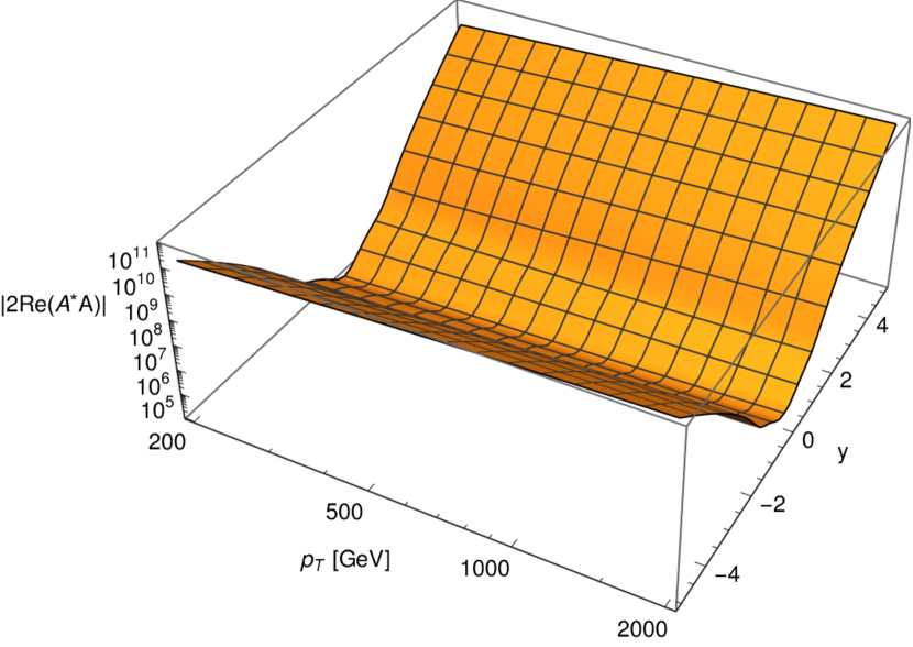
(a) $u\,\bar{u}\to g\,Z$

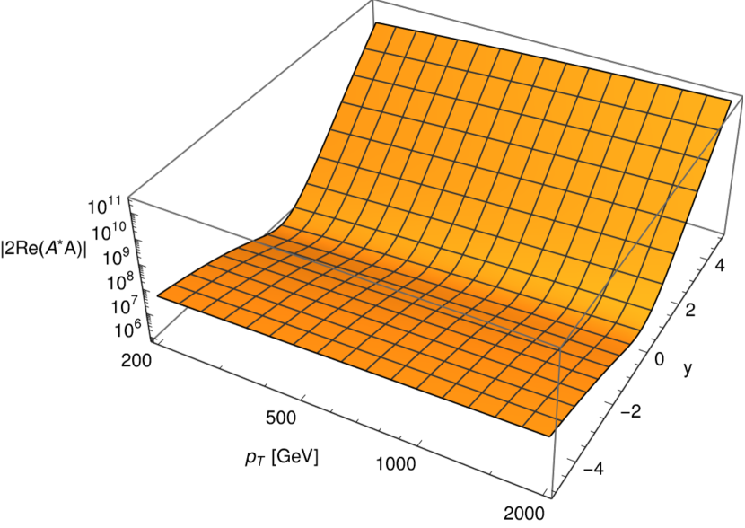
(b) $u\,g\to u\,Z$

(c) $d\,\bar{d}\to g\,Z$

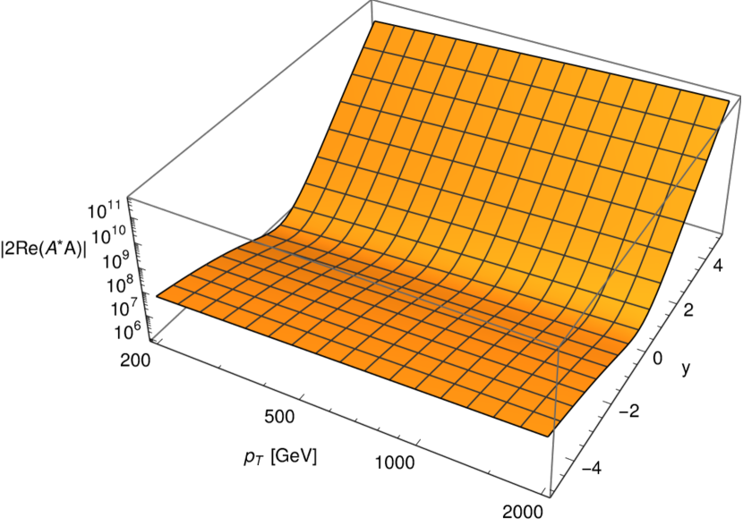
(d) $d\,g\to d\,Z$

Figure 2: Absolute value of the virtual NNLO finite remainders summed over colour and polarisations, see eq. 62, in all partonic channels as functions of transverse momentum $p_{t}$ and rapidity $y$ of the $Z$ boson. For simplicity, in this plot we set $\alpha_{s}=0.118$.

Finally, to illustrate the behaviour of the two-loop mixed QCD-EWK amplitudes across the whole kinematic coverage that we consider, in fig. 2 we plot

$$\left|\sum_{\rm col}\sum_{\rm pol}2\Re\left[\mathcal{A}^{(0,0)*}\mathcal{A}^{(1,1),\rm fin}\right]\right|,$$ (62)

see eq. 15, as a function of the $Z$-boson transverse momentum and rapidity, for all the independent partonic channels. The $(i,j)$ superscript in $\mathcal{A}^{(i,j)}$ indicates that only the $A^{(i,j)}$ contribution to eq. 15 is kept, see eq. 16. As it was the case for $\mathcal{M}^{\rm fin}$, the “fin” superscript implies that we only consider the finite part of the amplitude, as defined in sec. 4.

6 Conclusions and outlook

In this paper, we have performed a first important step towards the calculation of mixed QCD-EWK corrections for boosted $Z$ production in association with one hard jet. In particular, we have computed for the first time the bosonic contributions to the two-loop mixed QCD-EWK amplitudes. Our calculation relies on a recently proposed tensor decomposition method which reduces the redundancy stemming from unphysical dimensional regularization remnants. Moreover, we exploited the modern AMFlow method Liu:2022chg for highly efficient numerical evaluation of Feynman integrals. We have numerically evaluated the finite part of the two-loop amplitudes on a two-dimensional grid in $\{p_{t,Z},y_{Z}\}$ designed to offer good coverage for phenomenological investigations at the LHC and future colliders. We have performed extensive checks on our calculation, and expect the precision our final results to be more than sufficient for phenomenological applications. Our numerical evaluation of the tree-level, one-, and two-loop finite remainders in all the relevant partonic channels are provided in ancillary files.

Our framework is easily generalisable, and we expect it to be able to cope with the case of fermionic contribution as well, which we plan to investigate in the future. This would complete the calculation of the mixed QCD-EWK two-loop amplitudes for this process and will open the way for interesting investigations. In particular, one could apply these results to phenomenological studies at the LHC. This requires devising appropriate IR subtraction schemes for mixed QCD-QED real-emission, e.g. along the lines of ref. Buccioni:2022kgy . A successful completion of this programme would lead to a significant decrease on the theoretical uncertainty for important LHC analysis, like boosted Drell-Yan studies or monojet searches. It would also allow for a thorough study of the onset of the Sudakov regime, where EWK corrections are dominated by large logarithms. Insight in the transition region can provide important clues on the structure and size of subleading terms, and inform Sudakov-based approximations to mixed QCD-EWK corrections for more complicated processes. We leave these interesting avenues of exploration to the future.

Appendix A Projector coefficients

For convenience, we provide here an explicit form of the coefficients $c_{ik}$ required to define in eq. 21 the projectors $\mathcal{P}_{i}$ onto our Lorentz tensor basis $\overline{T}_{k}$.

$$\begin{split}c_{ik}&=\frac{1}{(d-3)\,tu}\times\\ &\left(\begin{array}[]{ccccccc}\frac{(s+u)^{2}}{2s^{2}}&-\frac{(s+u)^{2}}{2s^{2}t}&\frac{m_{Z}^{2}s-tu}{2s^{2}}&0&\frac{tu-m_{Z}^{2}s}{2s^{2}t}&0&0\\ -\frac{(s+u)^{2}}{2s^{2}t}&\frac{d(s+u)^{2}}{2s^{2}t^{2}}&\frac{tu-m_{Z}^{2}s}{2s^{2}t}&-\frac{u(s+u)}{2s^{2}t}&\frac{d(m_{Z}^{2}s-tu)+2t(u-s)}{2s^{2}t^{2}}&\frac{s+u}{2st}&0\\ \frac{m_{Z}^{2}s-tu}{2s^{2}}&\frac{tu-m_{Z}^{2}s}{2s^{2}t}&\frac{(s+t)^{2}}{2s^{2}}&0&-\frac{(s+t)^{2}}{2s^{2}t}&0&0\\ 0&-\frac{u(s+u)}{2s^{2}t}&0&\frac{u^{2}}{2s^{2}}&-\frac{u(s+t)}{2s^{2}t}&0&0\\ \frac{tu-m_{Z}^{2}s}{2s^{2}t}&\frac{d(m_{Z}^{2}s-tu)+2t(u-s)}{2s^{2}t^{2}}&-\frac{(s+t)^{2}}{2s^{2}t}&-\frac{u(s+t)}{2s^{2}t}&\frac{d(s+t)^{2}-4st}{2s^{2}t^{2}}&\frac{s-t}{2st}&0\\ 0&\frac{s+u}{2st}&0&0&\frac{s-t}{2st}&\frac{1}{2}&0\\ 0&0&0&0&0&0&\frac{1}{2(d-4)}\\ \end{array}\right),\end{split}$$ (63)

with $s=s_{12}$, $t=s_{13}$, $u=s_{23}$.

Appendix B Integral topologies

In this appendix we report the definition of the 18 basics topologies introduced in sec. 3.3. They read

$$\begin{split}\text{PL2A}&=\{k_{1}^{2},k_{2}^{2},(k_{1}-k_{2})^{2},(k_{1}-p_{1})^{2},(k_{2}-p_{1})^{2},(k_{1}-p_{12})^{2},(k_{2}-p_{12})^{2},(k_{1}-p_{123})^{2},(k_{2}-p_{123})^{2}\}\,,\\ \text{PL2Z1}&=\{k_{1}^{2}-m_{Z}^{2},k_{2}^{2},(k_{1}-k_{2})^{2},(k_{1}-p_{1})^{2},(k_{2}-p_{1})^{2},(k_{1}-p_{12})^{2},(k_{2}-p_{12})^{2},(k_{1}-p_{123})^{2},(k_{2}-p_{123})^{2}\}\,,\\ \text{PL2Z3}&=\{k_{1}^{2},k_{2}^{2},(k_{1}-k_{2})^{2}-m_{Z}^{2},(k_{1}-p_{1})^{2},(k_{2}-p_{1})^{2},(k_{1}-p_{12})^{2},(k_{2}-p_{12})^{2},(k_{1}-p_{123})^{2},(k_{2}-p_{123})^{2}\}\,,\\ \text{PL2Z4}&=\{k_{1}^{2},k_{2}^{2},(k_{1}-k_{2})^{2},-m_{Z}^{2}+(k_{1}-p_{1})^{2},(k_{2}-p_{1})^{2},(k_{1}-p_{12})^{2},(k_{2}-p_{12})^{2},(k_{1}-p_{123})^{2},(k_{2}-p_{123})^{2}\}\,,\\ \text{PL2W1}&=\{k_{1}^{2}-m_{W}^{2},k_{2}^{2},(k_{1}-k_{2})^{2},(k_{1}-p_{1})^{2},(k_{2}-p_{1})^{2},(k_{1}-p_{12})^{2},(k_{2}-p_{12})^{2},(k_{1}-p_{123})^{2},(k_{2}-p_{123})^{2}\}\,,\\ \text{PL2W3}&=\{k_{1}^{2},k_{2}^{2},(k_{1}-k_{2})^{2}-m_{W}^{2},(k_{1}-p_{1})^{2},(k_{2}-p_{1})^{2},(k_{1}-p_{12})^{2},(k_{2}-p_{12})^{2},(k_{1}-p_{123})^{2},(k_{2}-p_{123})^{2}\}\,,\\ \text{PL2W4}&=\{k_{1}^{2},k_{2}^{2},(k_{1}-k_{2})^{2},-m_{W}^{2}+(k_{1}-p_{1})^{2},(k_{2}-p_{1})^{2},(k_{1}-p_{12})^{2},(k_{2}-p_{12})^{2},(k_{1}-p_{123})^{2},(k_{2}-p_{123})^{2}\}\,,\\ \text{PL2W29}&=\{k_{1}^{2},k_{2}^{2}-m_{W}^{2},(k_{1}-k_{2})^{2},(k_{1}-p_{1})^{2},(k_{2}-p_{1})^{2},(k_{1}-p_{12})^{2},(k_{2}-p_{12})^{2},(k_{1}-p_{123})^{2},-m_{W}^{2}+(k_{2}-p_{123})^{2}\}\,,\\ \text{NPL2A}&=\{k_{1}^{2},k_{2}^{2},(k_{1}-k_{2})^{2},(k_{1}-p_{1})^{2},(k_{2}-p_{1})^{2},(k_{1}-p_{12})^{2},(k_{1}-k_{2}+p_{3})^{2},(k_{2}-p_{123})^{2},(k_{1}-k_{2}-p_{12})^{2}\}\,,\\ \text{NPL2Z1}&=\{k_{1}^{2}-m_{Z}^{2},k_{2}^{2},(k_{1}-k_{2})^{2},(k_{1}-p_{1})^{2},(k_{2}-p_{1})^{2},(k_{1}-p_{12})^{2},(k_{1}-k_{2}+p_{3})^{2},(k_{2}-p_{123})^{2},(k_{1}-k_{2}-p_{12})^{2}\}\,,\\ \text{NPL2Z4}&=\{k_{1}^{2},k_{2}^{2},(k_{1}-k_{2})^{2},-m_{Z}^{2}+(k_{1}-p_{1})^{2},(k_{2}-p_{1})^{2},(k_{1}-p_{12})^{2},(k_{1}-k_{2}+p_{3})^{2},(k_{2}-p_{123})^{2},(k_{1}-k_{2}-p_{12})^{2}\}\,,\\ \text{NPL2Z7}&=\{k_{1}^{2},k_{2}^{2},(k_{1}-k_{2})^{2},(k_{1}-p_{1})^{2},(k_{2}-p_{1})^{2},(k_{1}-p_{12})^{2},-m_{Z}^{2}+(k_{1}-k_{2}+p_{3})^{2},(k_{2}-p_{123})^{2},(k_{1}-k_{2}-p_{12})^{2}\}\,,\\ \text{NPL2Z1c13c24}&=\{k_{1}^{2}-m_{Z}^{2},k_{2}^{2},(k_{1}-k_{2})^{2},(k_{1}-p_{3})^{2},(k_{2}-p_{3})^{2},(k_{1}+p_{1}+p_{2})^{2},(k_{1}-k_{2}+p_{1})^{2},(k_{2}+p_{2})^{2},(k_{1}-k_{2}+p_{1}+p_{2})^{2}\}\,,\\ \text{NPL2W1}&=\{k_{1}^{2}-m_{W}^{2},k_{2}^{2},(k_{1}-k_{2})^{2},(k_{1}-p_{1})^{2},(k_{2}-p_{1})^{2},(k_{1}-p_{12})^{2},(k_{1}-k_{2}+p_{3})^{2},(k_{2}-p_{123})^{2},(k_{1}-k_{2}-p_{12})^{2}\}\,,\\ \text{NPL2W4}&=\{k_{1}^{2},k_{2}^{2},(k_{1}-k_{2})^{2},-m_{W}^{2}+(k_{1}-p_{1})^{2},(k_{2}-p_{1})^{2},(k_{1}-p_{12})^{2},(k_{1}-k_{2}+p_{3})^{2},(k_{2}-p_{123})^{2},(k_{1}-k_{2}-p_{12})^{2}\}\,,\\ \text{NPL2W7}&=\{k_{1}^{2},k_{2}^{2},(k_{1}-k_{2})^{2},(k_{1}-p_{1})^{2},(k_{2}-p_{1})^{2},(k_{1}-p_{12})^{2},-m_{W}^{2}+(k_{1}-k_{2}+p_{3})^{2},(k_{2}-p_{123})^{2},(k_{1}-k_{2}-p_{12})^{2}\}\,,\\ \text{NPL2W1c13c24}&=\{k_{1}^{2}-m_{W}^{2},k_{2}^{2},(k_{1}-k_{2})^{2},(k_{1}-p_{3})^{2},(k_{2}-p_{3})^{2},(k_{1}+p_{1}+p_{2})^{2},(k_{1}-k_{2}+p_{1})^{2},(k_{2}+p_{2})^{2},(k_{1}-k_{2}+p_{1}+p_{2})^{2}\}\,,\\ \text{NPL2W28}&=\{k_{1}^{2},k_{2}^{2}-m_{W}^{2},(k_{1}-k_{2})^{2},(k_{1}-p_{1})^{2},(k_{2}-p_{1})^{2},(k_{1}-p_{12})^{2},(k_{1}-k_{2}+p_{3})^{2},-m_{W}^{2}+(k_{2}-p_{123})^{2},(k_{1}-k_{2}-p_{12})^{2}\},\end{split}$$

where each list corresponds to $\{\mathcal{D}_{t,1},...,\mathcal{D}_{t,9}\}$, see sec. 3.3. For convenience, these topologies definitions are also provided in computer-readable format in an ancillary file.

References

- (1) ATLAS collaboration, Cross-section measurements for the production of a boson in association with high-transverse-momentum jets in collisions at TeV with the ATLAS detector, 2205.02597.
- (2) CMS collaboration, Measurement of differential cross sections for the production of a Z boson in association with jets in proton-proton collisions at = 13 TeV, 2205.02872.
- (3) J. M. Lindert et al., Precise predictions for jets dark matter backgrounds, Eur. Phys. J. C 77 (2017) 829, [1705.04664].
- (4) R. Boughezal, Y. Huang and F. Petriello, Exploring the SMEFT at dimension eight with Drell-Yan transverse momentum measurements, Phys. Rev. D 106 (2022) 036020, [2207.01703].
- (5) ATLAS collaboration, G. Aad et al., Search for new phenomena in events with an energetic jet and missing transverse momentum in collisions at =13 TeV with the ATLAS detector, Phys. Rev. D 103 (2021) 112006, [2102.10874].
- (6) CMS collaboration, A. Tumasyan et al., Search for new particles in events with energetic jets and large missing transverse momentum in proton-proton collisions at = 13 TeV, JHEP 11 (2021) 153, [2107.13021].
- (7) A. Gehrmann-De Ridder, T. Gehrmann, E. W. N. Glover, A. Huss and T. A. Morgan, Precise QCD predictions for the production of a Z boson in association with a hadronic jet, Phys. Rev. Lett. 117 (2016) 022001, [1507.02850].
- (8) A. Gehrmann-De Ridder, T. Gehrmann, E. W. N. Glover, A. Huss and T. A. Morgan, The NNLO QCD corrections to Z boson production at large transverse momentum, JHEP 07 (2016) 133, [1605.04295].
- (9) A. Gehrmann-De Ridder, T. Gehrmann, E. W. N. Glover, A. Huss and T. A. Morgan, NNLO QCD corrections for Drell-Yan and observables at the LHC, JHEP 11 (2016) 094, [1610.01843].
- (10) R. Boughezal, J. M. Campbell, R. K. Ellis, C. Focke, W. T. Giele, X. Liu et al., Z-boson production in association with a jet at next-to-next-to-leading order in perturbative QCD, Phys. Rev. Lett. 116 (2016) 152001, [1512.01291].
- (11) R. Boughezal, X. Liu and F. Petriello, Phenomenology of the Z-boson plus jet process at NNLO, Phys. Rev. D 94 (2016) 074015, [1602.08140].
- (12) R. Boughezal, C. Focke, X. Liu and F. Petriello, -boson production in association with a jet at next-to-next-to-leading order in perturbative QCD, Phys. Rev. Lett. 115 (2015) 062002, [1504.02131].
- (13) R. Boughezal, X. Liu and F. Petriello, W-boson plus jet differential distributions at NNLO in QCD, Phys. Rev. D 94 (2016) 113009, [1602.06965].
- (14) J. M. Campbell, R. K. Ellis and C. Williams, Direct Photon Production at Next-to–Next-to-Leading Order, Phys. Rev. Lett. 118 (2017) 222001, [1612.04333].
- (15) J. M. Campbell, R. K. Ellis and C. Williams, Driving missing data at the LHC: NNLO predictions for the ratio of and , Phys. Rev. D 96 (2017) 014037, [1703.10109].
- (16) T. Gehrmann, T. Peraro and L. Tancredi, Two-loop QCD corrections to the V → helicity amplitudes with axial-vector couplings, JHEP 02 (2023) 041, [2211.13596].
- (17) A. Denner, S. Dittmaier, T. Kasprzik and A. Muck, Electroweak corrections to dilepton + jet production at hadron colliders, JHEP 06 (2011) 069, [1103.0914].
- (18) A. Denner, S. Dittmaier, T. Kasprzik and A. Mück, Electroweak corrections to monojet production at the LHC, Eur. Phys. J. C 73 (2013) 2297, [1211.5078].
- (19) S. Kallweit, J. M. Lindert, P. Maierhofer, S. Pozzorini and M. Schönherr, NLO QCD+EW predictions for V + jets including off-shell vector-boson decays and multijet merging, JHEP 04 (2016) 021, [1511.08692].
- (20) A. Denner, S. Dittmaier, T. Kasprzik and A. Muck, Electroweak corrections to W + jet hadroproduction including leptonic W-boson decays, JHEP 08 (2009) 075, [0906.1656].
- (21) J. H. Kuhn and A. A. Penin, Sudakov logarithms in electroweak processes, hep-ph/9906545.
- (22) J. H. Kuhn, A. Kulesza, S. Pozzorini and M. Schulze, Electroweak corrections to hadronic photon production at large transverse momenta, JHEP 03 (2006) 059, [hep-ph/0508253].
- (23) J. H. Kuhn, A. Kulesza, S. Pozzorini and M. Schulze, One-loop weak corrections to hadronic production of Z bosons at large transverse momenta, Nucl. Phys. B 727 (2005) 368–394, [hep-ph/0507178].
- (24) J. H. Kuhn, A. Kulesza, S. Pozzorini and M. Schulze, Electroweak corrections to large transverse momentum production of W bosons at the LHC, Phys. Lett. B 651 (2007) 160–165, [hep-ph/0703283].
- (25) J. H. Kuhn, A. Kulesza, S. Pozzorini and M. Schulze, Electroweak corrections to hadronic production of W bosons at large transverse momenta, Nucl. Phys. B 797 (2008) 27–77, [0708.0476].
- (26) A. Behring, F. Buccioni, F. Caola, M. Delto, M. Jaquier, K. Melnikov et al., Mixed QCD-electroweak corrections to -boson production in hadron collisions, Phys. Rev. D 103 (2021) 013008, [2009.10386].
- (27) F. Buccioni, F. Caola, M. Delto, M. Jaquier, K. Melnikov and R. Röntsch, Mixed QCD-electroweak corrections to on-shell Z production at the LHC, Phys. Lett. B 811 (2020) 135969, [2005.10221].
- (28) S. Dittmaier, T. Schmidt and J. Schwarz, Mixed NNLO QCD×electroweak corrections of to single-W/Z production at the LHC, JHEP 12 (2020) 201, [2009.02229].
- (29) L. Buonocore, M. Grazzini, S. Kallweit, C. Savoini and F. Tramontano, Mixed QCD-EW corrections to at the LHC, Phys. Rev. D 103 (2021) 114012, [2102.12539].
- (30) R. Bonciani, L. Buonocore, M. Grazzini, S. Kallweit, N. Rana, F. Tramontano et al., Mixed Strong-Electroweak Corrections to the Drell-Yan Process, Phys. Rev. Lett. 128 (2022) 012002, [2106.11953].
- (31) F. Buccioni, F. Caola, H. A. Chawdhry, F. Devoto, M. Heller, A. von Manteuffel et al., Mixed QCD-electroweak corrections to dilepton production at the LHC in the high invariant mass region, JHEP 06 (2022) 022, [2203.11237].
- (32) A. Denner, S. Dittmaier, M. Roth and D. Wackeroth, Predictions for all processes e+ e- — 4 fermions + gamma, Nucl. Phys. B 560 (1999) 33–65, [hep-ph/9904472].
- (33) A. Denner, S. Dittmaier, M. Roth and L. H. Wieders, Electroweak corrections to charged-current e+ e- — 4 fermion processes: Technical details and further results, Nucl. Phys. B 724 (2005) 247–294, [hep-ph/0505042].
- (34) M. Beneke, A. P. Chapovsky, A. Signer and G. Zanderighi, Effective theory calculation of resonant high-energy scattering, Nucl. Phys. B 686 (2004) 205–247, [hep-ph/0401002].
- (35) A. H. Hoang and C. J. Reisser, Electroweak absorptive parts in NRQCD matching conditions, Phys. Rev. D 71 (2005) 074022, [hep-ph/0412258].
- (36) M. Beneke and V. A. Smirnov, Asymptotic expansion of Feynman integrals near threshold, Nucl. Phys. B 522 (1998) 321–344, [hep-ph/9711391].
- (37) A. Denner and S. Dittmaier, Electroweak Radiative Corrections for Collider Physics, Phys. Rept. 864 (2020) 1–163, [1912.06823].
- (38) T. Gehrmann and E. Remiddi, Analytic continuation of massless two loop four point functions, Nucl. Phys. B 640 (2002) 379–411, [hep-ph/0207020].
- (39) G. ’t Hooft and M. Veltman, Regularization and renormalization of gauge fields, Nuclear Physics B 44 (1972) 189–213.
- (40) Particle Data Group collaboration, R. L. Workman et al., Review of Particle Physics, PTEP 2022 (2022) 083C01.
- (41) T. Peraro and L. Tancredi, Physical projectors for multi-leg helicity amplitudes, JHEP 07 (2019) 114, [1906.03298].
- (42) T. Peraro and L. Tancredi, Tensor decomposition for bosonic and fermionic scattering amplitudes, Phys. Rev. D 103 (2021) 054042, [2012.00820].
- (43) R. G. Stuart, Gauge invariance, analyticity and physical observables at the Z0 resonance, Phys. Lett. B 262 (1991) 113–119.
- (44) A. Aeppli, G. J. van Oldenborgh and D. Wyler, Unstable particles in one loop calculations, Nucl. Phys. B 428 (1994) 126–146, [hep-ph/9312212].
- (45) S. Dittmaier and M. Huber, Radiative corrections to the neutral-current Drell-Yan process in the Standard Model and its minimal supersymmetric extension, JHEP 01 (2010) 060, [0911.2329].
- (46) S. Dittmaier, A. Huss and C. Schwinn, Dominant mixed QCD-electroweak O() corrections to Drell–Yan processes in the resonance region, Nucl. Phys. B 904 (2016) 216–252, [1511.08016].
- (47) L. J. Dixon, Calculating scattering amplitudes efficiently, in Theoretical Advanced Study Institute in Elementary Particle Physics (TASI 95): QCD and Beyond, 1, 1996. hep-ph/9601359.
- (48) P. Nogueira, Automatic Feynman graph generation, J. Comput. Phys. 105 (1993) 279–289.
- (49) A. von Manteuffel and C. Studerus, Reduze 2 - Distributed Feynman Integral Reduction, 1201.4330.
- (50) C. Studerus, Reduze-Feynman Integral Reduction in C++, Comput. Phys. Commun. 181 (2010) 1293–1300, [0912.2546].
- (51) J. A. M. Vermaseren, New features of FORM, math-ph/0010025.
- (52) K. G. Chetyrkin and F. V. Tkachov, Integration by Parts: The Algorithm to Calculate beta Functions in 4 Loops, Nucl. Phys. B 192 (1981) 159–204.
- (53) P. Maierhöfer, J. Usovitsch and P. Uwer, Kira—A Feynman integral reduction program, Comput. Phys. Commun. 230 (2018) 99–112, [1705.05610].
- (54) P. Maierhöfer and J. Usovitsch, Kira 1.2 Release Notes, 1812.01491.
- (55) S. Laporta, High precision calculation of multiloop Feynman integrals by difference equations, Int. J. Mod. Phys. A 15 (2000) 5087–5159, [hep-ph/0102033].
- (56) W. Decker, G.-M. Greuel, G. Pfister and H. Schönemann, “Singular 4-3-0 — A computer algebra system for polynomial computations.” http://www.singular.uni-kl.de, 2022.
- (57) M. Bonetti, E. Panzer, V. A. Smirnov and L. Tancredi, Two-loop mixed QCD-EW corrections to , JHEP 11 (2020) 045, [2007.09813].
- (58) M. Bonetti, E. Panzer and L. Tancredi, Two-loop mixed QCD-EW corrections to → Hg, qg → Hq, and → , JHEP 06 (2022) 115, [2203.17202].
- (59) A. V. Smirnov and V. A. Smirnov, How to choose master integrals, Nucl. Phys. B 960 (2020) 115213, [2002.08042].
- (60) J. Usovitsch, Factorization of denominators in integration-by-parts reductions, 2002.08173.
- (61) R. N. Lee, Presenting LiteRed: a tool for the Loop InTEgrals REDuction, 1212.2685.
- (62) R. N. Lee, LiteRed 1.4: a powerful tool for reduction of multiloop integrals, J. Phys. Conf. Ser. 523 (2014) 012059, [1310.1145].
- (63) A. von Manteuffel and R. M. Schabinger, A novel approach to integration by parts reduction, Phys. Lett. B 744 (2015) 101–104, [1406.4513].
- (64) T. Peraro, Scattering amplitudes over finite fields and multivariate functional reconstruction, JHEP 12 (2016) 030, [1608.01902].
- (65) T. Peraro, FiniteFlow: multivariate functional reconstruction using finite fields and dataflow graphs, JHEP 07 (2019) 031, [1905.08019].
- (66) X. Liu, Reconstruction of rational functions made simple, 2306.12262.
- (67) A. V. Kotikov, Differential equations method: New technique for massive Feynman diagrams calculation, Phys. Lett. B 254 (1991) 158–164.
- (68) M. Czakon, Tops from Light Quarks: Full Mass Dependence at Two-Loops in QCD, Phys. Lett. B 664 (2008) 307–314, [0803.1400].
- (69) X. Liu and Y.-Q. Ma, AMFlow: A Mathematica package for Feynman integrals computation via auxiliary mass flow, Comput. Phys. Commun. 283 (2023) 108565, [2201.11669].
- (70) X. Liu, Y.-Q. Ma and C.-Y. Wang, A Systematic and Efficient Method to Compute Multi-loop Master Integrals, Phys. Lett. B 779 (2018) 353–357, [1711.09572].
- (71) C. Brønnum-Hansen and C.-Y. Wang, Contribution of third generation quarks to two-loop helicity amplitudes for W boson pair production in gluon fusion, JHEP 01 (2021) 170, [2009.03742].
- (72) X. Liu and Y.-Q. Ma, Multiloop corrections for collider processes using auxiliary mass flow, Phys. Rev. D 105 (2022) L051503, [2107.01864].
- (73) X. Chen, X. Guan, C.-Q. He, X. Liu and Y.-Q. Ma, Heavy-quark-pair production at lepton colliders at NNNLO in QCD, 2209.14259.
- (74) X. Chen, X. Guan, C.-Q. He, Z. Li, X. Liu and Y.-Q. Ma, Complete two-loop electroweak corrections to , 2209.14953.
- (75) F. Febres Cordero, G. Figueiredo, M. Kraus, B. Page and L. Reina, Two-Loop Master Integrals for Leading-Color Amplitudes with a Light-Quark Loop, 2312.08131.
- (76) A. Denner, Techniques for calculation of electroweak radiative corrections at the one loop level and results for W physics at LEP-200, Fortsch. Phys. 41 (1993) 307–420, [0709.1075].
- (77) S. Catani, The Singular behavior of QCD amplitudes at two loop order, Phys. Lett. B 427 (1998) 161–171, [hep-ph/9802439].
- (78) J. M. Campbell, R. K. Ellis and W. T. Giele, A Multi-Threaded Version of MCFM, Eur. Phys. J. C 75 (2015) 246, [1503.06182].
- (79) F. Buccioni, J.-N. Lang, J. M. Lindert, P. Maierhöfer, S. Pozzorini, H. Zhang et al., OpenLoops 2, Eur. Phys. J. C 79 (2019) 866, [1907.13071].
- (80) L. W. Garland, T. Gehrmann, E. W. N. Glover, A. Koukoutsakis and E. Remiddi, Two loop QCD helicity amplitudes for e+ e- — three jets, Nucl. Phys. B 642 (2002) 227–262, [hep-ph/0206067].
- (81) Nicolas Deutschmann, “Qgraf-xml-drawer.”
- (82) J. Ellis, TikZ-Feynman: Feynman diagrams with TikZ, Comput. Phys. Commun. 210 (2017) 103–123, [1601.05437].