Simple and general bounds on quantum random access codes
Abstract
Random access codes are a type of communication task that is widely used in quantum information science. The optimal average success probability that can be achieved through classical strategies is known for any random access code. However, only a few cases are solved exactly for quantum random access codes. In this paper, we provide bounds for the fully general setting of independent variables, each selected from a -dimensional classical alphabet and encoded in a -dimensional quantum system subject to an arbitrary quantum measurement. The bound recovers the exactly known special cases, and we demonstrate numerically that even though the bound is not tight overall, it can still yield a good approximation.
I Introduction
Quantum random access codes are a broadly useful tool in quantum information science. In addition to being studied on their own merit (see e.g. [1, 2, 3, 4, 5, 6, 7, 8]), an incomplete list of their broader relevance includes protocols for quantum contextuality [9], information-theoretic principles for quantum correlations [10], tests of quantum dimension [11, 12], quantum cryptography [13], famous open problems in Hilbert space geometry [14] and certification of measurements [15, 16, 17] and instruments [18, 19].
Consider a communication scenario in which a sender encodes private data into a message that is sent to a receiver who wants to recover some freely chosen part of the original data set. RACs are a particularly natural class of such tasks. In a RAC, the private data can consist of independent and uniformly distributed classical variables, . Each variable is selected from an alphabet with distinct symbols, for . The data set is then encoded by the sender, Alice, into a typically much smaller message whose dimension is . The message is sent to the receiver, Bob, who privately selects at random which element in the data set he wishes to recover, labeled by , and outputs as his guess for the value of the random variable . The average success probability (ASP) of the RAC is hence given by
| (1) |
where, following a common short-hand notation, we used , and as labels of the corresponding random variables’ outcomes.
In a classical RAC, the message is represented by a random variable with possible integer values. The encoding is then represented by any function and, similarly, the decoding consists of a set of functions . The case in which the message dimension equals the size of the alphabet, i.e., when , has been the most studied case so far. The optimal ASP for such protocols was conjectured in [20] and later proven in [21]. In the general case, namely when , the optimal ASP was recently proven in [22].
In a quantum RAC, the sender encodes the classical data into a quantum state whose Hilbert space dimension is . The receiver’s decoding corresponds to a set of quantum measurements , for , where denotes the outcome and denotes the setting. For each , any -dimensional positive operator-valued measure (POVM) is a valid decoding operation. Hence, in the quantum RAC, the optimal ASP becomes
| (2) |
Finding the optimal quantum ASP is, in general, not easy. However, one family of exact results is known. This pertains to the case of and . It was conjectured in [20] and later proven in [23] that
| (3) |
This can be achieved by selecting the two decoding measurements as the computational and Fourier bases measurements. The encodings are obtained via the Weyl-Heisenberg group generators as , where and , with being a uniform superposition of and its Fourier transform [20]. This protocol is also unique, in a weaker self-testing sense: any pair of mutually unbiased bases leads to an optimal strategy, and not all of these are unitarily equivalent to the computational and Fourier bases [23].
One more exact result is known, namely when Alice has three bits and communicates a qubit to Bob. In that case, one has
| (4) |
The optimal quantum protocol consists in measuring the three Pauli observables and preparing eight qubit states on the Bloch sphere so that they form a cube [24, 25]. The protocol is known to be unique in a self-testing sense [26].
Beyond these exact results, a generic bound on the optimal quantum ASP when is known [27] to be
| (5) |
This was later generalized in [28] to a bound valid for arbitrary tuples , which reads
| (6) |
Eq. (6) reduces to Eq. (5) when and therefore subsumes that bound. Note that it does not recover the exact family of results in Eq. (3). Other known bounds for quantum RACs rely mainly on relaxation methods based on semidefinite programming (SDP) [29]. These are commonly applied to specific and typically small-scale tuples . See e.g., [30, 31, 32] for methods and case studies.
In this paper, we present two simple analytical upper bounds on the quantum ASP which apply to the most general setting, namely any tuple . Our final, combined, bound is given in Corollary 1. It is distinct from the known general bound in Eq. (6). Notably, it recovers the both exact results in Eq. (3) and Eq. (4) as special cases, as well as the bound in Eq. (5). Since our bound is typically not tight, we study its performance through numerical case studies. We demonstrate with examples that it can be a good approximation of the exact value.
II Bounds on quantum average success probability
We introduce a lemma before presenting the first main result.
Lemma 1.
Let be a trace-zero Hermitian matrix. Then it holds that
| (7) |
where is the rank of , and denote the operator and the Frobenius norms, respectively.
Proof.
Matrix has real eigenvalues which we denote as . Since , we have that . Let be the largest eigenvalue in the absolute value, which implies that . The Frobenius norm can then be lower-bounded as
| (8) |
In the first inequality we used the well-known relation , where is the trace norm and is the dimension of the relevant operator. In the second inequality we discarded the absolute values, and in the next step we used the trace-zero condition. Re-arranging the left- and right-hand side returns Eq. (7). ∎
We now state and prove our first bound on the quantum ASP.
Result 1.
The average success probability of the quantum random access code, in the setting of -element data set with alphabet size and message dimension , is bounded as
| (9) |
Proof.
We can trivially re-write the quantum ASP in Eq. (2) as
| (10) |
where we omitted writing the maximization and limits of the sums for convenience. In Eq. (10), is the identity operator on the -dimensional Hilbert space in which and are defined. From the normalization, , it follows that the first term evaluates to . Clearly, the optimal choice of corresponds to the eigenvector with the largest eigenvalue of the Hermitian operator . This gives
| (11) |
Notice that by adopting the form (10), we have conveniently ensured that . Hence, we can now apply Lemma 1 to obtain
| (12) |
where in the second step we used the concavity inequality , which holds for any , . Simplifying the expression under the square-root gives
| (13) |
The two terms on the right-hand-side of Eq. (13) simplify, respectively, as
| (14) | ||||
and
| (15) | ||||
where in the last inequality we used that for , we have . In the above two equations, denotes the summation over and such that . Substituting this back into Eq. (13), we obtain
| (16) |
where we used that for an operator , we have . Finally, substituting this back into Eq. (12) returns the result in Eq. (9). ∎
Notice that when , we recover the known bound (5). Also, when , we recover the previously known bound in Eq. (6). However, for and the above upper bound coincides with the other known bound (3) only for , and otherwise provides a weaker bound.
We now state and prove the second main result, which is a different general bound on the quantum ASP. This time, it is more relevant for the scaling in , as it recovers the bound in Eq. (3) as a special case. In this sense, it is complementary to Result 1.
Result 2.
The average success probability of the quantum random access code, in the setting of -element data set with alphabet size and message dimension , is bounded as
| (17) |
Proof.
Our main tool is an operator inequality proved by Popovici and Sebestyén [33]. For a set of positive semidefinite matrices , it holds that
| (18) |
where is an matrix with elements . Applying this to the quantum ASP we get
| (19) |
where , for . Let us now fix the computational basis on , and separate the diagonal and off-diagonal parts of matrices ,
| (20) |
where, as before, is the summation over and such that . Applying the triangle inequality gives
| (21) |
The completeness condition of POVMs implies for all , which when applied to the first term above bounds it by . Substituting the above into the right-hand-side of Eq. (19), we arrive at
| (22) |
Notice now that the operators are Hermitian and trace-zero. Hence we can apply Lemma 1 to bound the operator norm by the Frobenius norm. This gives
| (23) |
Bounding the operator norm by the Frobenius norm again, but this time without the trace-zero condition, and therefore without the rank pre-factor, and then using the concavity of the square-root function as well as the completeness condition, we get
| (24) | ||||
which is the final result. ∎
Combining the bounds in Result 1 and Result 2, the our final bound on the quantum ASP becomes simply the smallest of the two, which is summarized by the following Corollary.
Corollary 1.
The average success probability of the quantum random access code, in the setting of -element data set with alphabet size and message dimension , is bounded as
| (25) |
In particular, for the case , the two expressions are identical. For the case and , we have that
| (26) |
which corresponds to the first bound in Eq. (25), and for and , we have that
| (27) |
which corresponds to the second bound in Eq. (25).
When applied to the special cases of and , the bound in Corollary 1 reduces to the previously known bounds in Eq. (5) and Eq. (3). The bound in Corollary 1 and the other known generic bound, given in Eq. (6), admit no strict hierarchy. That is, there exist tuples for which one of the bounds performs better than the other. For instance, when and , the two bounds are identical, while for , Corollary 1 provides a tighter bound. This is also the case when . On the other hand, for and a sufficiently large , Eq. (6) is a tighter bound. In general, the best known bound can be easily determined for each particular case.
III Numerical case studies
In this section, we present numerical bounds on the quantum ASP for some families of RACs in order to benchmark our analytic bounds. We present both, lower bounds to see the possible gap between our analytic results and the actual optimal ASP, and upper bounds to prove that in some cases our bounds can be improved.
We use the seesaw SDP algorithms to derive lower bounds on the quantum ASP. Note that the ASP (2) is linear in both and in . Consequently, for a fixed POVM operators , optimizing the ASP over the set of is an SDP. Similarly, for a fixed set of , optimizing the ASP over is again an SDP. The seesaw algorithm starts with a randomly selected set of , and finds the optimal for that set as the solution of an SDP. Then found in the first iteration are fixed, and the optimal for this set of POVMs are found via an SDP. This process is iterated until the value of the ASP converges to a locally optimal value up to some error threshold. This method is not guaranteed to find a global maximum, but every set of and found by this algorithm provide a valid lower bound on the ASP.
The performance of the seesaw algorithm is highly dependent on the initialization, i.e., on the randomly selected . To obtain the lower bounds in this paper, in our numerical calculations we sample random pure states uniformly (with respect to the Haar measure) and repeat the algorithm a fixed number of times. Since there is no guarantee that the produced estimate is unbiased, one cannot determine a sufficient number of random initialization of the seesaw algorithm. Nevertheless, by observing the distribution of the local optima produced by the seesaw algorithm for a number of random initializations, one can judge about optimality of the produced lower bounds.
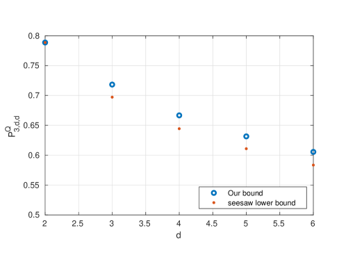
Since the case of and has been the focus of study for some time [14] and this family is unsolved apart from , in Fig. 1 we compare lower bounds from seesaw techniques with our analytic bound from Corollary 1, which correspond to Eq. (27) because we have , for values . We also include the point for , for which the seesaw algorithm finds the known optimal ASP. This plot demonstrates that our bound is possibly not tight for these values of , but the gap between the lower bound from the seesaw algorithm and our upper bound is seemingly not too large. That is, our upper bounds provide a reasonable approximation of the optimal quantum ASP from above.
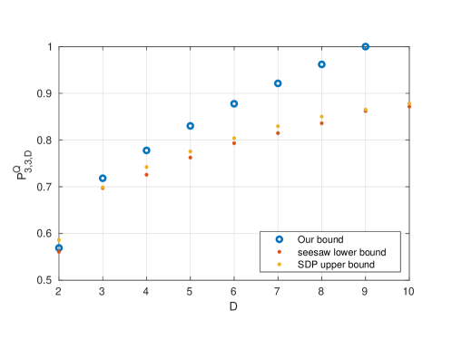
The smallest unsolved case of quantum RAC is , for which the best lower bound, both analytically and numerically, is given by performing measurements in three MUBs, and choosing the corresponding optimal states [14, 34]. This gives the lower bound , and our analytic upper bound is , according to Eq. (27). In order to test the tightness of our analytic upper bound, we numerically computed upper bounds on using SDP techniques, in particular using the QDimSum package [35] to implement the techniques described in [30, 31]. Note that this technique, as implemented in [35], assumes that the measurements used are projective. While there is no evidence that projective measurements are not optimal for the case, the upper bounds provided by this technique may be lower than the actual maximum.
Loosely speaking, the method [30] relies on moment matrices indexed by monomials of the operators and . The more monomials are used for building the moment matrix, the tighter the upper bound, leading to a hierarchy of upper bounds. On level 1 of the hierarchy, only order-1 monomials are used, that is, the monomials . On level 2, all order-2 monomials are used, that is, the monomials
| (28) |
One can also define “intermediate” levels, for example, the level “”, using the monomials
| (29) |
Using this notation, the upper bounds we found for the various levels of the SDP hierarchy for are given in Table 1.
| Level | Upper bound on |
| 1 | 0.7182 |
| 0.6989 | |
| 2 | 0.6989 |
| 0.6989 | |
| 0.69855 | |
| 0.69853 |
Note that our analytic bound is recovered, up to the solver precision, for level of the hierarchy. Then, various consecutive levels yield the same upper bound, which, interestingly, corresponds to the hypothetical case of measuring in three orthonormal bases , and on that form a set of MUBs with the triple products
| (30) |
being uniform, even though such bases are known not to exist [34]. Note that these triple products are naturally related to Bargmann invariants [36]. Adding certain order- monomials, such as and , makes the upper bound tighter, with our current best numerical upper bound being , which shows that there is still room for an improvement when deriving analytic upper bounds.
We also compare our analytical bounds to other recently developed SDP techniques [32]. In particular, a special case of the bounds developed in [32] corresponds to upper bounds on . Importantly, these do not assume that the measurements are projective. In Figure 2 we plot the seesaw lower bound, our analytical upper bound, and the upper bound from Ref. [32] on for . These numerical results show that our bound is not tight for this family of RACs apart from the case, where our analytical upper bound is actually tighter than the one obtained in Ref. [32].
Lastly, we compare our analytical upper bounds with seesaw lower bounds in the case for various different values for and in Table 2. While our bound is potentially not tight apart from the case, it provides a good approximation of the quantum optimal ASP for generic values of and .
| Seesaw lower bound | Our upper bound | |
| (2,2) | 0.78868 | 0.78868 |
| (2,3) | 0.80794∗ | 0.91068 |
| (2,4) | 0.90825 | 1 |
| (3,2) | 0.56066 | 0.56904 |
| (3,3) | 0.69715 | 0.71823 |
| (3,4) | 0.72567 | 0.77778 |
| (3,5) | 0.76241 | 0.83024 |
| (4,2) | 0.43697 | 0.45412 |
| (4,3) | 0.47525 | 0.58333 |
| (4,4) | 0.64434 | 0.66667 |
| (4,5) | 0.66331∗ | 0.70601 |
IV Conclusions
In this paper, we derive a universal analytic upper bound on the average success probability of quantum random access codes. We consider the most general case of RACs with independent variables from a -dimensional alphabet encoded into a -dimensional quantum system, for arbitrary and . Our bounds recover known families of upper bounds for the case of and , which is known to be tight [23], and the case, which is known to be tight for and [27]. In the general case, our bounds are not tight, although numerical evidence suggests that they provide reasonably good approximations of the actual quantum maximum. For the interesting case of , we show numerically that our upper bounds can be improved, and that the question whether MUBs measurements are optimal for this case is still unresolved. We believe that our bounds, in combination with that obtained in [28], will be useful for the analytical treatment of problems where RACs are used as a tool for benchmarking quantum information protocols.
Note that both of our bounds in Result 1 and 2 rely on pairwise properties of the measurements. In particular, both of these bounds at some point involve Hilbert-Schmidt inner products of measurement effects, and are, in principle, maximized when these inner products are uniform as both bounds use the concavity of the square root function. This would imply that if MUBs are indeed optimal for RACs, then any set of MUBs should give rise to the optimal ASP, as all sets of MUBs satisfy the above trace uniformity condition. It is known, however, that not all sets of MUBs give rise to the same ASP when [14, 34]. This implies that either MUBs are not optimal for RACs in the general case, or that new upper bounds relying on more than pairwise properties of measurement are needed to prove optimality.
Acknowledgements.
We thank Marcin Pawłowski for the years of insightful discussions about the subject of this paper. We thank Julio de Vicente for a valuable feedback. A.T. is supported by the Knut and Alice Wallenberg Foundation through the Wallenberg Center for Quantum Technology (WACQT) and the Swedish Research Council under Contract No. 2023-03498. This research was funded by the Deutsche Forschungsgemeinschaft (DFG, German Research Foundation), project number 441423094.References
- Nayak [1999] A. Nayak, Optimal lower bounds for quantum automata and random access codes, in 40th Annual Symposium on Foundations of Computer Science (Cat. No.99CB37039) (1999) pp. 369–376.
- Hayashi et al. [2006] M. Hayashi, K. Iwama, H. Nishimura, R. Raymond, and S. Yamashita, (4,1)-quantum random access coding does not exist—one qubit is not enough to recover one of four bits, New Journal of Physics 8, 129 (2006).
- Pawłowski and Żukowski [2010] M. Pawłowski and M. Żukowski, Entanglement-assisted random access codes, Phys. Rev. A 81, 042326 (2010).
- Tavakoli et al. [2016] A. Tavakoli, B. Marques, M. Pawłowski, and M. Bourennane, Spatial versus sequential correlations for random access coding, Phys. Rev. A 93, 032336 (2016).
- Liabøtrø [2017] O. Liabøtrø, Improved classical and quantum random access codes, Phys. Rev. A 95, 052315 (2017).
- Doriguello and Montanaro [2021] J. F. Doriguello and A. Montanaro, Quantum Random Access Codes for Boolean Functions, Quantum 5, 402 (2021).
- Miao et al. [2022] R.-H. Miao, Z.-D. Liu, Y.-N. Sun, C.-X. Ning, C.-F. Li, and G.-C. Guo, High-dimensional multi-input quantum random access codes and mutually unbiased bases, Phys. Rev. A 106, 042418 (2022).
- da Silva and Marques [2023] R. A. da Silva and B. Marques, Semidefinite-programming-based optimization of quantum random access codes over noisy channels, Phys. Rev. A 107, 042433 (2023).
- Spekkens et al. [2009] R. W. Spekkens, D. H. Buzacott, A. J. Keehn, B. Toner, and G. J. Pryde, Preparation contextuality powers parity-oblivious multiplexing, Phys. Rev. Lett. 102, 010401 (2009).
- Pawłowski et al. [2009] M. Pawłowski, T. Paterek, D. Kaszlikowski, V. Scarani, A. Winter, and M. Żukowski, Information causality as a physical principle, Nature 461, 1101 (2009).
- Brunner et al. [2013] N. Brunner, M. Navascués, and T. Vértesi, Dimension witnesses and quantum state discrimination, Phys. Rev. Lett. 110, 150501 (2013).
- Tavakoli et al. [2021] A. Tavakoli, J. Pauwels, E. Woodhead, and S. Pironio, Correlations in entanglement-assisted prepare-and-measure scenarios, PRX Quantum 2, 040357 (2021).
- Pawłowski and Brunner [2011] M. Pawłowski and N. Brunner, Semi-device-independent security of one-way quantum key distribution, Phys. Rev. A 84, 010302 (2011).
- Aguilar et al. [2018] E. A. Aguilar, J. J. Borkała, P. Mironowicz, and M. Pawłowski, Connections between mutually unbiased bases and quantum random access codes, Phys. Rev. Lett. 121, 050501 (2018).
- Mironowicz and Pawłowski [2019] P. Mironowicz and M. Pawłowski, Experimentally feasible semi-device-independent certification of four-outcome positive-operator-valued measurements, Phys. Rev. A 100, 030301 (2019).
- Tavakoli et al. [2020] A. Tavakoli, M. Smania, T. Vértesi, N. Brunner, and M. Bourennane, Self-testing nonprojective quantum measurements in prepare-and-measure experiments, Science Advances 6, eaaw6664 (2020), https://www.science.org/doi/pdf/10.1126/sciadv.aaw6664 .
- Carmeli et al. [2020] C. Carmeli, T. Heinosaari, and A. Toigo, Quantum random access codes and incompatibility of measurements, Europhysics Letters 130, 50001 (2020).
- Mohan et al. [2019] K. Mohan, A. Tavakoli, and N. Brunner, Sequential random access codes and self-testing of quantum measurement instruments, New Journal of Physics 21, 083034 (2019).
- Miklin et al. [2020] N. Miklin, J. J. Borkała, and M. Pawłowski, Semi-device-independent self-testing of unsharp measurements, Phys. Rev. Res. 2, 033014 (2020).
- Tavakoli et al. [2015] A. Tavakoli, A. Hameedi, B. Marques, and M. Bourennane, Quantum random access codes using single -level systems, Phys. Rev. Lett. 114, 170502 (2015).
- Ambainis et al. [2015] A. Ambainis, D. Kravchenko, and A. Rai, Optimal classical random access codes using single d-level systems (2015), arXiv:1510.03045 [quant-ph] .
- Saha et al. [2023] D. Saha, D. Das, A. K. Das, B. Bhattacharya, and A. S. Majumdar, Measurement incompatibility and quantum advantage in communication, Phys. Rev. A 107, 062210 (2023).
- Farkas and Kaniewski [2019] M. Farkas and J. Kaniewski, Self-testing mutually unbiased bases in the prepare-and-measure scenario, Phys. Rev. A 99, 032316 (2019).
- Ambainis et al. [1999] A. Ambainis, A. Nayak, A. Ta-Shma, and U. Vazirani, Dense quantum coding and a lower bound for 1-way quantum automata, in Proceedings of the Thirty-First Annual ACM Symposium on Theory of Computing, STOC ’99 (Association for Computing Machinery, New York, NY, USA, 1999) p. 376–383.
- Ambainis et al. [2002] A. Ambainis, A. Nayak, A. Ta-Shma, and U. Vazirani, Dense quantum coding and quantum finite automata, J. ACM 49, 496–511 (2002).
- Tavakoli et al. [2018] A. Tavakoli, J. Kaniewski, T. Vértesi, D. Rosset, and N. Brunner, Self-testing quantum states and measurements in the prepare-and-measure scenario, Phys. Rev. A 98, 062307 (2018).
- Ambainis et al. [2009] A. Ambainis, D. Leung, L. Mancinska, and M. Ozols, Quantum random access codes with shared randomness (2009), arXiv:0810.2937 [quant-ph] .
- de Vicente [2019] J. I. de Vicente, A general bound for the dimension of quantum behaviours in the prepare-and-measure scenario, Journal of Physics A: Mathematical and Theoretical 52, 095304 (2019).
- Tavakoli et al. [2023] A. Tavakoli, A. Pozas-Kerstjens, P. Brown, and M. Araújo, Semidefinite programming relaxations for quantum correlations (2023), arXiv:2307.02551 [quant-ph] .
- Navascués et al. [2015] M. Navascués, A. Feix, M. Araújo, and T. Vértesi, Characterizing finite-dimensional quantum behavior, Phys. Rev. A 92, 042117 (2015).
- Tavakoli et al. [2019] A. Tavakoli, D. Rosset, and M.-O. Renou, Enabling computation of correlation bounds for finite-dimensional quantum systems via symmetrization, Phys. Rev. Lett. 122, 070501 (2019).
- Pauwels et al. [2022] J. Pauwels, S. Pironio, E. Woodhead, and A. Tavakoli, Almost qudits in the prepare-and-measure scenario, Phys. Rev. Lett. 129, 250504 (2022).
- Popovici and Sebestyén [2006] D. Popovici and Z. Sebestyén, Norm estimations for finite sums of positive operators, Journal of Operator Theory 56, 3 (2006).
- Farkas [2017] M. Farkas, -fold unbiased bases: an extension of the MUB condition (2017), arXiv:1706.04446 [quant-ph] .
- [35] Qdimsum package.
- Chruściński and Jamiołkowski [2004] D. Chruściński and A. Jamiołkowski, Geometric Phases in Classical and Quantum Mechanics (Birkhäuser Boston, 2004).
