DUSt3R: Geometric 3D Vision Made Easy

Abstract

Multi-view stereo reconstruction (MVS) in the wild requires to first estimate the camera parameters e.g. intrinsic and extrinsic parameters. These are usually tedious and cumbersome to obtain, yet they are mandatory to triangulate corresponding pixels in 3D space, which is the core of all best performing MVS algorithms. In this work, we take an opposite stance and introduce DUSt3R, a radically novel paradigm for Dense and Unconstrained Stereo 3D Reconstruction of arbitrary image collections, i.e. operating without prior information about camera calibration nor viewpoint poses. We cast the pairwise reconstruction problem as a regression of pointmaps, relaxing the hard constraints of usual projective camera models. We show that this formulation smoothly unifies the monocular and binocular reconstruction cases. In the case where more than two images are provided, we further propose a simple yet effective global alignment strategy that expresses all pairwise pointmaps in a common reference frame. We base our network architecture on standard Transformer encoders and decoders, allowing us to leverage powerful pretrained models. Our formulation directly provides a 3D model of the scene as well as depth information, but interestingly, we can seamlessly recover from it, pixel matches, relative and absolute cameras. Exhaustive experiments on all these tasks showcase that the proposed DUSt3R can unify various 3D vision tasks and set new SoTAs on monocular/multi-view depth estimation as well as relative pose estimation. In summary, DUSt3R makes many geometric 3D vision tasks easy.

1 Introduction

Unconstrained image-based dense 3D reconstruction from multiple views is one of a few long-researched end-goals of computer vision [24, 89, 71]. In a nutshell, the task aims at estimating the 3D geometry and camera parameters of a particular scene, given a set of photographs of this scene. Not only does it have numerous applications like mapping [72, 13] , navigation [15], archaeology [86, 132], cultural heritage preservation [38], robotics [78], but perhaps more importantly, it holds a fundamentally special place among all 3D vision tasks. Indeed, it subsumes nearly all of the other geometric 3D vision tasks. Thus, modern approaches for 3D reconstruction consists in assembling the fruits of decades of advances in various sub-fields such as keypoint detection [62, 96, 26, 28] and matching [99, 119, 10, 59], robust estimation [3, 10, 180], Structure-from-Motion (SfM) and Bundle Adjustment (BA) [20, 105, 58], dense Multi-View Stereo (MVS) [106, 175, 157, 138], etc.

In the end, modern SfM and MVS pipelines boil down to solving a series of minimal problems: matching points, finding essential matrices, triangulating points, sparsely reconstructing the scene, estimating cameras and finally performing dense reconstruction. Considering recent advances, this rather complex chain is of course a viable solution in some settings [76, 142, 31, 162, 70, 145, 147], yet we argue it is quite unsatisfactory: each sub-problem is not solved perfectly and adds noise to the next step, increasing the complexity and the engineering effort required for the pipeline to work as a whole. In this regard, the absence of communication between each sub-problem is quite telling: it would seem more reasonable if they helped each other, i.e. dense reconstruction should naturally benefit from the sparse scene that was built to recover camera poses, and vice-versa. On top of that, key steps in this pipeline are brittle and prone to break in many cases [58]. For instance, the crucial stage of SfM that serves to estimate all camera parameters, is typically known to fail in many common situations, e.g. when the number of scene views is low [108], for objects with non-Lambertian surfaces [16], in case of insufficient camera motion [13], etc. This is concerning, because in the end, “an MVS algorithm is only as good as the quality of the input images and camera parameters” [32].

In this paper, we present DUSt3R, a radically novel approach for Dense Unconstrained Stereo 3D Reconstruction from un-calibrated and un-posed cameras. The main component is a network that can regress a dense and accurate scene representation solely from a pair of images, without prior information regarding the scene nor the cameras (not even the intrinsic parameters). The resulting scene representation is based on 3D pointmaps with rich properties: they simultaneously encapsulate (a) the scene geometry, (b) the relation between pixels and scene points and (c) the relation between the two viewpoints. From this output alone, practically all scene parameters (i.e. cameras and scene geometry) can be straightforwardly extracted. This is possible because our network jointly processes the input images and the resulting 3D pointmaps, thus learning to associate 2D structures with 3D shapes, and having the opportunities of solving multiple minimal problems simultaneously, enabling internal ‘collaboration’ between them.

Our model is trained in a fully-supervised manner using a simple regression loss, leveraging large public datasets for which ground-truth annotations are either synthetically generated [103, 68], reconstructed from SfM softwares [55, 161] or captured using dedicated sensors [93, 121, 165, 25]. We drift away from the trend of integrating task-specific modules [164], and instead adopt a fully data-driven strategy based on a generic transformer architecture, not enforcing any geometric constraints at inference, but being able to benefit from powerful pretraining schemes. The network learns strong geometric and shape priors, which are reminiscent of those commonly leveraged in MVS, like shape from texture, shading or contours [110].

To fuse predictions from multiple images pairs, we revisit bundle adjustment (BA) for the case of pointmaps, hereby achieving full-scale MVS. We introduce a global alignment procedure that, contrary to BA, does not involve minimizing reprojection errors. Instead, we optimize the camera pose and geometry alignment directly in 3D space, which is fast and shows excellent convergence in practice. Our experiments show that the reconstructions are accurate and consistent between views in real-life scenarios with various unknown sensors. We further demonstrate that the same architecture can handle real-life monocular and multi-view reconstruction scenarios seamlessly. Examples of reconstructions are shown in Fig. 1 and in the accompanying video.

In summary, our contributions are fourfold. First, we present the first holistic end-to-end 3D reconstruction pipeline from un-calibrated and un-posed images, that unifies monocular and binocular 3D reconstruction. Second, we introduce the pointmap representation for MVS applications, that enables the network to predict the 3D shape in a canonical frame, while preserving the implicit relationship between pixels and the scene. This effectively drops many constraints of the usual perspective camera formulation. Third, we introduce an optimization procedure to globally align pointmaps in the context of multi-view 3D reconstruction. Our procedure can extract effortlessly all usual intermediary outputs of the classical SfM and MVS pipelines. In a sense, our approach unifies all 3D vision tasks and considerably simplifies over the traditional reconstruction pipeline, making DUSt3R seem simple and easy in comparison. Fourth, we demonstrate promising performance on a range of 3D vision tasks In particular, our all-in-one model achieves state-of-the-art results on monocular and multi-view depth benchmarks, as well as multi-view camera pose estimation.

2 Related Work

For the sake of space, we summarize here the most related works in 3D vision, and refer the reader to the appendix in Sec.  for a more comprehensive review.

Structure-from-Motion (SfM) [44, 47, 20, 21, 105] aims at reconstructing sparse 3D maps while jointly determining camera parameters from a set of images. The traditional pipeline starts from pixel correspondences obtained from keypoint matching [42, 62, 5, 98, 4] between multiple images to determine geometric relationships, followed by bundle adjustment to optimize 3D coordinates and camera parameters jointly. Recently, the SfM pipeline has undergone substantial enhancements, particularly with the incorporation of learning-based techniques into its subprocesses. These improvements encompass advanced feature description [166, 26, 28, 96, 134], more accurate image matching [99, 119, 125, 17, 59, 81, 144, 3], featuremetric refinement [58], and neural bundle adjustment [57, 152]. Despite these advancements, the sequential structure of the SfM pipeline persists, making it vulnerable to noise and errors in each individual component.

MultiView Stereo (MVS) is the task of densely reconstructing visible surfaces, which is achieved via triangulation between multiple viewpoints. In the classical formulation of MVS, all camera parameters are supposed to be provided as inputs. The fully handcrafted [32, 174, 34, 106, 146], the more recent scene optimization based [75, 76, 142, 31, 162, 70, 145, 147], or learning based [52, 160, 179, 163, 85, 64] approaches all depend on camera parameter estimates obtained via complex calibration procedures, either during the data acquisition [1, 108, 23, 165] or using Structure-from-Motion approaches [105, 47] for in-the-wild reconstructions. Yet, in real-life scenarios, the inaccuracy of pre-estimated camera parameters can be detrimental for these algorithms to work properly. In this work, we propose instead to directly predict the geometry of visible surfaces without any explicit knowledge of the camera parameters.

Direct RGB-to-3D. Recently, some approaches aiming at directly predicting 3D geometry from a single RGB image have been proposed. Since the problem is by nature ill-posed without introducing additional assumptions, these methods leverage neural networks that learn strong 3D priors from large datasets to solve ambiguities. These methods can be classified into two groups. The first group leverages class-level object priors. For instance, Pavllo et al. [84, 82, 83] propose to learn a model that can fully recover shape, pose, and appearance from a single image, given a large collection of 2D images. While this type of approach is powerful, it does not allow to infer shape on objects from unseen categories. A second group of work, closest to our method, focuses instead on general scenes. These methods systematically build on or re-use existing monocular depth estimation (MDE) networks [90, 170, 6, 168]. Depth maps indeed encode a form of 3D information and, combined with camera intrinsics, can straightforwardly yield pixel-aligned 3D point-clouds. SynSin [150], for example, performs new viewpoint synthesis from a single image by rendering feature-augmented depthmaps knowing all camera parameters. Without camera intrinsics, one solution is to infer them by exploiting temporal consistency in video frames, either by enforcing a global alignment et al. [155] or by leveraging differentiable rendering with a photometric reconstruction loss [116, 36]. Another way is to explicitly learn to predict camera intrinsics, which enables to perform metric 3D reconstruction from a single image when combined with MDE [167, 169]. All these methods are, however, intrinsically limited by the quality of depth estimates, which arguably is ill-posed for monocular settings.

In contrast, our network processes two viewpoints simultaneously in order to output depthmaps, or rather, pointmaps. In theory, at least, this makes triangulation between rays from different viewpoint possible. Multi-view networks for 3D reconstruction have been proposed in the past. They are essentially based on the idea of building a differentiable SfM pipeline, replicating the traditional pipeline but training it end-to-end [135, 130, 183]. For that, however, ground-truth camera intrinsics are required as input, and the output is generally a depthmap and a relative camera pose [135, 183]. In contrast, our network has a generic architecture and outputs pointmaps, i.e. dense 2D field of 3D points, which handle camera poses implicitly and makes the regression problem much better posed.

Pointmaps. Using a collection of pointmaps as shape representation is quite counter-intuitive for MVS, but its usage is widespread for Visual Localization tasks, either in scene-dependent optimization approaches [8, 9, 11] or scene-agnostic inference methods [123, 158, 95]. Similarly, view-wise modeling is a common theme in monocular 3D reconstruction works [112, 56, 126, 140] and in view synthesis works [150]. The idea being to store the canonical 3D shape in multiple canonical views to work in image space. These approaches usually leverage explicit perspective camera geometry, via rendering of the canonical representation.

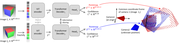
Figure 2: Architecture of the network $\mathcal{F}$. Two views of a scene $(I^{1},I^{2})$ are first encoded in a Siamese manner with a shared ViT encoder. The resulting token representations $F^{1}$ and $F^{2}$ are then passed to two transformer decoders that constantly exchange information via cross-attention. Finally, two regression heads output the two corresponding pointmaps and associated confidence maps. Importantly, the two pointmaps are expressed in the same coordinate frame of the first image $I^{1}$. The network $\mathcal{F}$ is trained using a simple regression loss (Eq. 4)

3 Method

Before delving into the details of our method, we introduce below the essential concept of pointmaps.

Pointmap. In the following, we denote a dense 2D field of 3D points as a pointmap $X\in\mathbb{R}^{W\times H\times 3}$. In association with its corresponding RGB image $I$ of resolution $W\times H$, $X$ forms a one-to-one mapping between image pixels and 3D scene points, i.e. $I_{i,j}\leftrightarrow X_{i,j}$, for all pixel coordinates $(i,j)\in\{1\ldots W\}\times\{1\ldots H\}$. We assume here that each camera ray hits a single 3D point, i.e. ignoring the case of translucent surfaces.

Cameras and scene. Given the camera intrinsics $K\in\mathbb{R}^{3\times 3}$, the pointmap $X$ of the observed scene can be straightforwardly obtained from the ground-truth depthmap $D\in\mathbb{R}^{W\times H}$ as $X_{i,j}=K^{-1}\left[iD_{i,j},jD_{i,j},D_{i,j}\right]^{\top}$. Here, $X$ is expressed in the camera coordinate frame. In the following, we denote as $X^{n,m}$ the pointmap $X^{n}$ from camera $n$ expressed in camera $m$’s coordinate frame:

$$X^{n,m}=P_{m}P_{n}^{-1}h\left(X^{n}\right)\vspace{-2mm}$$ (1)

with $P_{m},P_{n}\in\mathbb{R}^{3\times 4}$ the world-to-camera poses for images $n$ and $m$, and $h:(x,y,z)\rightarrow(x,y,z,1)$ the homogeneous mapping.

3.1 Overview

We wish to build a network that solves the 3D reconstruction task for the generalized stereo case through direct regression. To that aim, we train a network $\mathcal{F}$ that takes as input 2 RGB images $I^{1},I^{2}\in\mathbb{R}^{W\times H\times 3}$ and outputs 2 corresponding pointmaps $X^{1,1},X^{2,1}\in\mathbb{R}^{W\times H\times 3}$ with associated confidence maps $C^{1,1},C^{2,1}\in\mathbb{R}^{W\times H}$. Note that both pointmaps are expressed in the same coordinate frame of $I^{1}$, which radically differs from existing approaches but offers key advantages (see Secs. 1, 2, 3.3 and 3.4). For the sake of clarity and without loss of generalization, we assume that both images have the same resolution $W\times H$, but naturally in practice their resolution can differ.

Network architecture. The architecture of our network $\mathcal{F}$ is inspired by CroCo [149], making it straightforward to heavily benefit from CroCo pretraining [148]. As shown in Fig. 2, it is composed of two identical branches (one for each image) comprising each an image encoder, a decoder and a regression head. The two input images are first encoded in a Siamese manner by the same weight-sharing ViT encoder [27], yielding two token representations $F^{1}$ and $F^{2}$:

$$F^{1}=\text{Encoder}(I^{1}),F^{2}=\text{Encoder}(I^{2}).\vspace{-2mm}$$

The network then reasons over both of them jointly in the decoder. Similarly to CroCo [149], the decoder is a generic transformer network equipped with cross attention. Each decoder block thus sequentially performs self-attention (each token of a view attends to tokens of the same view), then cross-attention (each token of a view attends to all other tokens of the other view), and finally feeds tokens to a MLP. Importantly, information is constantly shared between the two branches during the decoder pass. This is crucial in order to output properly aligned pointmaps. Namely, each decoder block attends to tokens from the other branch:

$$G_{i}^{1}=\text{DecoderBlock}^{1}_{i}\left(G_{i-1}^{1},G_{i-1}^{2}\right),$$

$$G_{i}^{2}=\text{DecoderBlock}^{2}_{i}\left(G_{i-1}^{2},G_{i-1}^{1}\right),\vspace{-3mm}$$

for $i=1,\ldots,B$ for a decoder with $B$ blocks and initialized with encoder tokens $G_{0}^{1}:=F^{1}$ and $G_{0}^{2}:=F^{2}$. Here, $\text{DecoderBlock}_{i}^{v}(G^{1},G^{2})$ denotes the $i$-th block in branch $v\in\{1,2\}$, $G^{1}$ and $G^{2}$ are the input tokens, with $G^{2}$ the tokens from the other branch. Finally, in each branch a separate regression head takes the set of decoder tokens and outputs a pointmap and an associated confidence map:

$$X^{1,1},C^{1,1}=\text{Head}^{1}\left(G_{0}^{1},\ldots,G_{B}^{1}\right),$$

$$X^{2,1},C^{2,1}=\text{Head}^{2}\left(G_{0}^{2},\ldots,G_{B}^{2}\right).$$

Discussion. The output pointmaps $X^{1,1}$ and $X^{2,1}$ are regressed up to an unknown scale factor. Also, it should be noted that our generic architecture never explicitly enforces any geometrical constraints. Hence, pointmaps do not necessarily correspond to any physically plausible camera model. Rather, we let the network learn all relevant priors present from the train set, which only contains geometrically consistent pointmaps. Using a generic architecture allows to leverage strong pretraining technique, ultimately surpassing what existing task-specific architectures can achieve. We detail the learning process in the next section.

3.2 Training Objective

3D Regression loss. Our sole training objective is based on regression in the 3D space. Let us denote the ground-truth pointmaps as $\bar{X}^{1,1}$ and $\bar{X}^{2,1}$, obtained from Eq. 1 along with two corresponding sets of valid pixels $\mathcal{D}^{1},\mathcal{D}^{2}\subseteq\{1\ldots W\}\times\{1\ldots H\}$ on which the ground-truth is defined. The regression loss for a valid pixel $i\in\mathcal{D}^{v}$ in view $v\in\{1,2\}$ is simply defined as the Euclidean distance:

$$\ell_{\text{regr}}(v,i)=\left\|\frac{1}{z}X^{v,1}_{i}-\frac{1}{\bar{z}}\bar{X}^{v,1}_{i}\right\|.\vspace{-1mm}$$ (2)

To handle the scale ambiguity between prediction and ground-truth, we normalize the predicted and ground-truth pointmaps by scaling factors $z=\text{norm}(X^{1,1},X^{2,1})$ and $\bar{z}=\text{norm}(\bar{X}^{1,1},\bar{X}^{2,1})$, respectively, which simply represent the average distance of all valid points to the origin:

$$\text{norm}(X^{1},X^{2})=\frac{1}{|\mathcal{D}^{1}|+|\mathcal{D}^{2}|}\sum_{v\in\{1,2\}}\,\sum_{i\in\mathcal{D}^{v}}\left\|X^{v}_{i}\right\|.\vspace{-2mm}$$ (3)

Confidence-aware loss. In reality, and contrary to our assumption, there are ill-defined 3D points, e.g. in the sky or on translucent objects. More generally, some parts in the image are typically harder to predict that others. We thus jointly learn to predict a score for each pixel which represents the confidence that the network has about this particular pixel. The final training objective is the confidence-weighted regression loss from Eq. 2 over all valid pixels:

$$\mathcal{L}_{\text{conf}}=\sum_{v\in\{1,2\}}\,\sum_{i\in\mathcal{D}^{v}}C^{v,1}_{i}\ell_{\text{regr}}(v,i)-\alpha\log C^{v,1}_{i},\vspace{-2mm}$$ (4)

where $C^{v,1}_{i}$ is the confidence score for pixel $i$, and $\alpha$ is a hyper-parameter controlling the regularization term [136]. To ensure a strictly positive confidence, we typically define $C^{v,1}_{i}=1+\exp\widetilde{C^{v,1}_{i}}>1$. This has the effect of forcing the network to extrapolate in harder areas, e.g. like those ones covered by a single view. Training network $\mathcal{F}$ with this objective allows to estimate confidence scores without an explicit supervision. Examples of input image pairs with their corresponding outputs are shown in Fig. 3 and in the appendix in Figs. 4, 5 and 8.

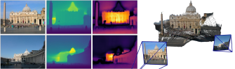
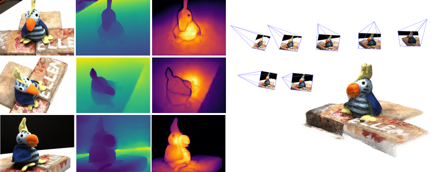
Figure 3: Reconstruction examples on two scenes never seen during training. From left to right: RGB, depth map, confidence map, reconstruction. The left scene shows the raw result output from $\mathcal{F}(I^{1},I^{2})$. The right scene shows the outcome of global alignment (Sec. 3.4).

3.3 Downstream Applications

The rich properties of the output pointmaps allows us to perform various convenient operations with relative ease.

Point matching. Establishing correspondences between pixels of two images can be trivially achieved by nearest neighbor (NN) search in the 3D pointmap space. To minimize errors, we typically retain reciprocal (mutual) correspondences $\mathcal{M}_{1,2}$ between images $I^{1}$ and $I^{2}$, i.e. we have:

$$\mathcal{M}_{1,2}=\{(i,j)\ |\ i=\text{NN}_{1}^{1,2}(j)\text{ and }j=\text{NN}_{1}^{2,1}(i)\}$$

$$\text{with }\text{NN}_{k}^{n,m}(i)=\operatorname*{arg\,min}_{j\in\{0,\ldots,WH\}}\left\|X^{n,k}_{j}-X^{m,k}_{i}\right\|.$$

Recovering intrinsics. By definition, the pointmap $X^{1,1}$ is expressed in $I^{1}$’s coordinate frame. It is therefore possible to estimate the camera intrinsic parameters by solving a simple optimization problem. In this work, we assume that the principal point is approximately centered and pixel are squares, hence only the focal $f_{1}^{*}$ remains to be estimated:

$$f_{1}^{*}=\operatorname*{arg\,min}_{f_{1}}\sum_{i=0}^{W}\sum_{j=0}^{H}C^{1,1}_{i,j}\left\|(i^{\prime},j^{\prime})-f_{1}\frac{(X^{1,1}_{i,j,0},X^{1,1}_{i,j,1})}{X^{1,1}_{i,j,2}}\right\|,\vspace{-1mm}$$

with $i^{\prime}=i-\frac{W}{2}$ and $j^{\prime}=j-\frac{H}{2}$. Fast iterative solvers, e.g. based on the Weiszfeld algorithm [87], can find the optimal $f_{1}^{*}$ in a few iterations. For the focal $f_{2}^{*}$ of the second camera, the simplest option is to perform the inference for the pair $(I^{2},I^{1})$ and use above formula with $X^{2,2}$ instead of $X^{1,1}$.

Relative pose estimation can be achieved in several fashions. One way is to perform 2D matching and recover intrinsics as described above, then estimate the Epipolar matrix and recover the relative pose [44]. Another, more direct, way is to compare the pointmaps $X^{1,1}\leftrightarrow X^{1,2}$ (or, equivalently, $X^{2,2}\leftrightarrow X^{1,2}$) using Procrustes alignment [63] to get the relative pose $P^{*}=[R^{*}|t^{*}]$:

$$R^{*},t^{*}=\operatorname*{arg\,min}_{\sigma,R,t}\sum_{i}C^{1,1}_{i}C^{1,2}_{i}\left\|\sigma(RX^{1,1}_{i}+t)-X^{1,2}_{i}\right\|^{2},\vspace{-2mm}$$

which can be achieved in closed-form. Procrustes alignment is, unfortunately, sensitive to noise and outliers. A more robust solution is finally to rely on RANSAC [30] with PnP [44, 51].

Absolute pose estimation, also termed visual localization, can likewise be achieved in several different ways. Let $I^{Q}$ denote the query image and $I^{B}$ the reference image for which 2D-3D correspondences are available. First, intrinsics for $I^{Q}$ can be estimated from $X^{Q,Q}$. One possibility consists of obtaining 2D correspondences between $I^{Q}$ and $I^{B}$, which in turn yields 2D-3D correspondences for $I^{Q}$, and then running PnP-RANSAC [30, 51]. Another solution is to get the relative pose between $I^{Q}$ and $I^{B}$ as described previously. Then, we convert this pose to world coordinate by scaling it appropriately, according to the scale between $X^{B,B}$ and the ground-truth pointmap for $I^{B}$.

3.4 Global Alignment

The network $\mathcal{F}$ presented so far can only handle a pair of images. We now present a fast and simple post-processing optimization for entire scenes that enables the alignment of pointmaps predicted from multiple images into a joint 3D space. This is possible thanks to the rich content of our pointmaps, which encompasses by design two aligned point-clouds and their corresponding pixel-to-3D mapping.

Pairwise graph. Given a set of images $\{I^{1},I^{2},\ldots,I^{N}\}$ for a given scene, we first construct a connectivity graph $\mathcal{G}(\mathcal{V},\mathcal{E})$ where $N$ images form vertices $\mathcal{V}$ and each edge $e=(n,m)\in\mathcal{E}$ indicates that images $I^{n}$ and $I^{m}$ shares some visual content. To that aim, we either use existing off-the-shelf image retrieval methods, or we pass all pairs through network $\mathcal{F}$ (inference takes $\approx$40ms on a H100 GPU) and measure their overlap based on the average confidence in both pairs, then we filter out low-confidence pairs.

Global optimization. We use the connectivity graph $\mathcal{G}$ to recover globally aligned pointmaps $\{\chi^{n}\in\mathbb{R}^{W\times H\times 3}\}$ for all cameras $n=1\ldots N$. To that aim, we first predict, for each image pair $e=(n,m)\in\mathcal{E}$, the pairwise pointmaps $X^{n,n},X^{m,n}$ and their associated confidence maps $C^{n,n},C^{m,n}$. For the sake of clarity, let us define $X^{n,e}:=X^{n,n}$ and $X^{m,e}:=X^{m,n}$. Since our goal involves to rotate all pairwise predictions in a common coordinate frame, we introduce a pairwise pose $P_{e}\in\mathbb{R}^{3\times 4}$ and scaling $\sigma_{e}>0$ associated to each pair $e\in\mathcal{E}$. We then formulate the following optimization problem:

$$\chi^{*}=\operatorname*{arg\,min}_{\chi,P,\sigma}\sum_{e\in\mathcal{E}}\sum_{v\in e}\sum_{i=1}^{HW}C^{v,e}_{i}\left\|\chi_{i}^{v}-\sigma_{e}P_{e}X^{v,e}_{i}\right\|.\vspace{-3mm}$$ (5)

Here, we abuse notation and write $v\in e$ for $v\in\{n,m\}$ if $e=(n,m)$. The idea is that, for a given pair $e$, the same rigid transformation $P_{e}$ should align both pointmaps $X^{n,e}$ and $X^{m,e}$ with the world-coordinate pointmaps $\chi^{n}$ and $\chi^{m}$, since $X^{n,e}$ and $X^{m,e}$ are by definition both expressed in the same coordinate frame. To avoid the trivial optimum where $\sigma_{e}=0,\,\forall e\in\mathcal{E}$, we enforce that $\prod_{e}\sigma_{e}=1$.

Recovering camera parameters. A straightforward extension to this framework enables to recover all cameras parameters. By simply replacing $\chi^{n}_{i,j}:=P_{n}^{-1}h(K_{n}^{-1}[iD^{n}_{i,j};jD^{n}_{i,j};D^{n}_{i,j}])$ (i.e. enforcing a standard camera pinhole model as in Eq. 1), we can thus estimate all camera poses $\{P_{n}\}$, associated intrinsics $\{K_{n}\}$ and depthmaps $\{D^{n}\}$ for $n=1\ldots N$.

Discussion. We point out that, contrary to traditional bundle adjustment, this global optimization is fast and simple to perform in practice. Indeed, we are not minimizing 2D reprojection errors, as bundle adjustment normally does, but 3D projection errors. The optimization is carried out using standard gradient descent and typically converges after a few hundred steps, requiring mere seconds on a standard GPU.

4 Experiments with DUSt3R

Training data. We train our network with a mixture of eight datasets: Habitat [103], MegaDepth [55], ARKitScenes [25], MegaDepth [55], Static Scenes 3D [68], Blended MVS [161], ScanNet++ [165], CO3D-v2 [93] and Waymo [121]. These datasets feature diverse scenes types: indoor, outdoor, synthetic, real-world, object-centric, etc. When image pairs are not directly provided with the dataset, we extract them based on the method described in [148]. Specifically, we utilize off-the-shelf image retrieval and point matching algorithms to match and verify image pairs. All in all, we extract 8.5M pairs in total.

Training details. During each epoch, we randomly sample an equal number of pairs from each dataset to equalize disparities in dataset sizes. We wish to feed relatively high-resolution images to our network, say 512 pixels in the largest dimension. To mitigate the high cost associated with such input, we train our network sequentially, first on 224$\times$224 images and then on larger 512-pixel images. We randomly select the image aspect ratios for each batch (e.g. 16/9, 4/3, etc), so that at test time our network is familiar with different image shapes. We simply crop images to the desired aspect-ratio, and resize so that the largest dimension is 512 pixels.

We use standard data augmentation techniques and training set-up overall. Our network architecture comprises a Vit-Large for the encoder [27], a ViT-Base for the decoder and a DPT head [90]. We refer to the appendix in Sec.  for more details on the training and architecture. Before training, we initialize our network with the weights of an off-the-shelf CroCo pretrained model [148]. Cross-View completion (CroCo) is a recently proposed pretraining paradigm inspired by MAE [45] that has been shown to excel on various downstream 3D vision tasks, and is thus particularly suited to our framework. We ablate in Sec. 4.6 the impact of CroCo pretraining and increase in image resolution.

Evaluation. In the remainder of this section, we benchmark DUSt3R on a representative set of classical 3D vision tasks, each time specifying datasets, metrics and comparing performance with existing state-of-the-art approaches. We emphasize that all results are obtained with the same DUSt3R model (our default model is denoted as ‘DUSt3R 512’, other DUSt3R models serves for the ablations in Section Sec. 4.6), i.e. we never finetune our model on a particular downstream task. During test, all test images are rescaled to 512px while preserving their aspect ratio. Since there may exist different ‘routes’ to extract task-specific outputs from DUSt3R, as described in Sec. 3.3 and Sec. 3.4, we precise each time the employed method.

Qualitative results. DUSt3R yields high-quality dense 3D reconstructions even in challenging situations. We refer the reader to the appendix in Sec.  for non-cherrypicked visualizations of pairwise and multi-view reconstructions.

4.1 Visual Localization

Methods

7Scenes (Indoor) [113]

Cambridge (Outdoor) [48]

Chess

Fire

Heads

Office

Pumpkin

Kitchen

Stairs

S. Facade

O. Hospital

K. College

St.Mary’s

G. Court

FM

AS [102]

4/1.96

3/1.53

2/1.45

9/3.61

8/3.10

7/3.37

3/2.22

4/0.21

20/0.36

13/0.22

8/0.25

24/0.13

HLoc  [100]

2/0.79

2/0.87

2/0.92

3/0.91

5/1.12

4/1.25

6/1.62

4/0.2

15/0.3

12/0.20

7/0.21

11/0.16

E2E

DSAC* [11]

2/1.10

2/1.24

1/1.82

3/1.15

4/1.34

4/1.68

3/1.16

5/0.3

15/0.3

15/0.3

13/0.4

49/0.3

HSCNet [54]

2/0.7

2/0.9

1/0.9

3/0.8

4/1.0

4/1.2

3/0.8

6/0.3

19/0.3

18/0.3

9/0.3

28/0.2

PixLoc [101]

2/0/80

2/0.73

1/0.82

3/0.82

4/1.21

3/1.20

5/1.30

5/0.23

16/0.32

14/0.24

10/0.34

30/0.14

SC-wLS [151]

3/0.76

5/1.09

3/1.92

6/0.86

8/1.27

9/1.43

12/2.80

11/0.7

42/1.7

14/0.6

39/1.3

164/0.9

NeuMaps  [124]

2/0.81

3/1.11

2/1.17

3/0.98

4/1.11

4/1.33

4/1.12

6/0.25

19/0.36

14/0.19

17/0.53

6/ 0.10

DUSt3R 224-NoCroCo

5/1.76

6/2.02

3/1.75

5/1.54

9/2.35

6/1.82

34/7.81

24/1.33

79/1.17

69/1.15

46/1.51

143/1.32

DUSt3R 224

3/0.96

3/1.02

1/1.00

4/1.04

5/1.26

4/1.36

21/4.08

9/0.38

26/0.46

20/0.32

11/0.38

36/0.24

DUSt3R 512

3/0.97

3/0.95

2/1.37

3/1.01

4/1.14

4/1.34

11/2.84

6/0.26

17/0.33

11/0.20

7/0.24

38/0.16

Table 1: Absolute camera pose on 7Scenes [113] and Cambridge-Landmarks [48] datasets. We report the median translation and rotation errors ($cm/^{\circ}$) to feature matching (FM) based and end-to-end (E2E) learning-base methods. The best results at each category are in bold.

Datasets and metrics. We first evaluate DUSt3R for the task of absolute pose estimation on the 7Scenes [113] and Cambridge Landmarks datasets [48]. 7Scenes contains 7 indoor scenes with RGB-D images from videos and their 6-DOF camera poses. Cambridge-Landmarks contains 6 outdoor scenes with RGB images and their associated camera poses, which are obtained via SfM. We report the median translation and rotation errors in (cm/^∘), respectively.

Protocol and results. To compute camera poses in world coordinates, we use DUSt3R as a 2D-2D pixel matcher (see Section 3.3) between a query and the most relevant database images obtained using off-the-shelf image retrieval AP-GeM [94]. In other words, we simply use the raw pointmaps output from $\mathcal{F}(I^{Q},I^{B})$ without any refinement, where $I^{Q}$ is the query image and $I^{B}$ is a database image. We use the top 20 retrieved images for Cambridge-Landmarks and top 1 for 7Scenes and leverage the known query intrinsics. For results obtained without using ground-truth intrinsics parameters, refer to the appendix in Sec. .

We compare our results against the state of the art in Table 1 for each scene of the two datasets. Our method obtains comparable accuracy compared to existing approaches, being feature-matching ones [102, 100] or end-to-end learning-based methods [11, 54, 101, 151, 124], even managing to outperform strong baselines like HLoc [100] in some cases. We believe this to be significant for two reasons. First, DUSt3R was never trained for visual localisation in any way. Second, neither query image nor database images were seen during DUSt3R’s training.

4.2 Multi-view Pose Estimation

We now evaluate DUSt3R on multi-view relative pose estimation after the global alignment from Sec. 3.4.

Datasets. Following  [139], we use two multi-view datasets, CO3Dv2 [93] and RealEstate10k [185] for the evaluation. CO3Dv2 contains 6 million frames extracted from approximately 37k videos, covering 51 MS-COCO categories. The ground-truth camera poses are annotated using COLMAP from 200 frames in each video. RealEstate10k is an indoor/outdoor dataset with 10 million frames from about 80K video clips on YouTube, the camera poses being obtained by SLAM with bundle adjustment. We follow the protocol introduced in [139] to evaluate DUSt3R on 41 categories from CO3Dv2 and 1.8K video clips from the test set of RealEstate10k. For each sequence, we random select 10 frames and feed all possible 45 pairs to DUSt3R.

Baselines and metrics. We compare DUSt3R pose estimation results, obtained either from PnP-RANSAC or global alignment, against the learning-based RelPose [176], PoseReg [139] and PoseDiffusion [139], and structure-based PixSFM [58], COLMAP+SPSG (COLMAP [106] extended with SuperPoint [26] and SuperGlue [99]). Similar to [139], we report the Relative Rotation Accuracy (RRA) and Relative Translation Accuracy (RTA) for each image pair to evaluate the relative pose error and select a threshold $\tau=15$ to report RTA@$15$ and RRA$@15$. Additionally, we calculate the mean Average Accuracy (mAA)$@30$, defined as the area under the curve accuracy of the angular differences at $min({\rm RRA}@30,{\rm RTA}@30)$.

Results. As shown in Table 2, DUSt3R with global alignment achieves the best overall performance on the two datasets and significantly surpasses the state-of-the-art PoseDiffusion [139]. Moreover, DUSt3R with PnP also demonstrates superior performance over both learning and structure-based existing methods. It is worth noting that RealEstate10K results reported for PoseDiffusion are from the model trained on CO3Dv2. Nevertheless, we assert that our comparison is justified considering that RealEstate10K is not used either during DUSt3R’s training. We also report performance with less input views (between 3 and 10) in the appendix (Sec. ), in which case DUSt3R also yields excellent performance on both benchmarks.

		Outdoor				Indoor
Methods	Train	DDAD[40]		KITTI [35]		BONN [79]		NYUD-v2 [114]		TUM [118]
		Rel$\downarrow$	$\delta_{1.25}\uparrow$	Rel$\downarrow$	$\delta_{1.25}\uparrow$	Rel$\downarrow$	$\delta_{1.25}\uparrow$	Rel$\downarrow$	$\delta_{1.25}\uparrow$	$\operatorname{Rel}\downarrow$	$\delta_{1.25}\uparrow$
DPT-BEiT[90]	D	10.70	84.63	9.45	89.27	-	-	5.40	96.54	10.45	89.68
NeWCRFs[173]	D	9.59	82.92	5.43	91.54	-	-	6.22	95.58	14.63	82.95
Monodepth2 [37]	SS	23.91	75.22	11.42	86.90	56.49	35.18	16.19	74.50	31.20	47.42
SC-SfM-Learners [6]	SS	16.92	77.28	11.83	86.61	21.11	71.40	13.79	79.57	22.29	64.30
SC-DepthV3 [120]	SS	14.20	81.27	11.79	86.39	12.58	88.92	12.34	84.80	16.28	79.67
MonoViT[181]	SS	-	-	09.92	90.01	-	-	-	-	-
RobustMIX [91]	T	-	-	18.25	76.95	-	-	11.77	90.45	15.65	86.59
SlowTv [116]	T	12.63	79.34	(6.84)	(56.17)	-	-	11.59	87.23	15.02	80.86
DUSt3R 224-NoCroCo	T	19.63	70.03	20.10	71.21	14.44	86.00	14.51	81.06	22.14	66.26
DUSt3R 224	T	16.32	77.58	16.97	77.89	11.05	89.95	10.28	88.92	17.61	75.44
DUSt3R 512	T	13.88	81.17	10.74	86.60	8.08	93.56	6.50	94.09	14.17	79.89

Methods	Co3Dv2 [93]				RealEstate10K
	RRA@15	RTA@15	mAA(30)		mAA(30)
RelPose [176]	57.1	-	-		-
Colmap+SPSG [26, 99]	36.1	27.3	25.3		45.2
PixSfM [58]	33.7	32.9	30.1		49.4
PosReg [139]	53.2	49.1	45.0		-
PoseDiffusion  [139]	80.5	79.8	66.5		48.0
DUSt3R 512 (w/ PnP)	94.3	88.4	77.2		61.2
DUSt3R 512 (w/ GA)	96.2	86.8	76.7		67.7

Table 2: Left: Monocular depth estimation on multiple benchmarks. D-Supervised, SS-Self-supervised, T-transfer (zero-shot). (Parentheses) refers to training on the same set. Right: Multi-view pose regression on the CO3Dv2 [93] and RealEst10K [185] with 10 random frames.

Methods		GT	GT	GT	Align	KITTI		ScanNet		ETH3D		DTU		T&T		Average
		Pose	Range	Intrinsics		rel $\downarrow$	$\tau\uparrow$	rel $\downarrow$	$\tau\uparrow$	rel $\downarrow$	$\tau\uparrow$	rel $\downarrow$	$\tau\uparrow$	rel$\downarrow$	$\tau\uparrow$	rel$\downarrow$	$\tau\uparrow$	time (s)$\downarrow$
(a)	COLMAP [105, 106]	$\checkmark$	$\times$	$\checkmark$	$\times$	12.0	58.2	14.6	34.2	16.4	55.1	0.7	96.5	2.7	95.0	9.3	67.8	$\approx$ 3 min
	COLMAP Dense [105, 106]	$\checkmark$	$\times$	$\checkmark$	$\times$	26.9	52.7	38.0	22.5	89.8	23.2	20.8	69.3	25.7	76.4	40.2	48.8	$\approx$ 3 min
(b)	MVSNet [160]	$\checkmark$	$\checkmark$	$\checkmark$	$\times$	22.7	36.1	24.6	20.4	35.4	31.4	(1.8)	$(86.0)$	8.3	73.0	18.6	49.4	0.07
	MVSNet Inv. Depth [160]	$\checkmark$	$\checkmark$	$\checkmark$	$\times$	18.6	30.7	22.7	20.9	21.6	35.6	(1.8)	$(86.7)$	6.5	74.6	14.2	49.7	0.32
	Vis-MVSSNet [175]	$\checkmark$	$\checkmark$	$\checkmark$	$\times$	9.5	55.4	8.9	33.5	10.8	43.3	(1.8)	(87.4)	4.1	87.2	7.0	61.4	0.70
	MVS2D ScanNet [159]	$\checkmark$	$\checkmark$	$\checkmark$	$\times$	21.2	8.7	(27.2)	(5.3)	27.4	4.8	17.2	9.8	29.2	4.4	24.4	6.6	0.04
	MVS2D DTU [159]	$\checkmark$	$\checkmark$	$\checkmark$	$\times$	226.6	0.7	32.3	11.1	99.0	11.6	(3.6)	(64.2)	25.8	28.0	77.5	23.1	0.05
(c)	DeMon [135]	$\checkmark$	$\times$	$\checkmark$	$\times$	16.7	13.4	75.0	0.0	19.0	16.2	23.7	11.5	17.6	18.3	30.4	11.9	0.08
	DeepV2D KITTI [130]	$\checkmark$	$\times$	$\checkmark$	$\times$	(20.4)	(16.3)	25.8	8.1	30.1	9.4	24.6	8.2	38.5	9.6	27.9	10.3	1.43
	DeepV2D ScanNet [130]	$\checkmark$	$\times$	$\checkmark$	$\times$	61.9	5.2	(3.8)	(60.2)	18.7	28.7	9.2	27.4	33.5	38.0	25.4	31.9	2.15
	MVSNet [160]	$\checkmark$	$\times$	$\checkmark$	$\times$	14.0	35.8	1568.0	5.7	507.7	8.3	(4429.1)	(0.1)	118.2	50.7	1327.4	20.1	0.15
	MVSNet Inv. Depth [160]	$\checkmark$	$\times$	$\checkmark$	$\times$	29.6	8.1	65.2	28.5	60.3	5.8	(28.7)	(48.9)	51.4	14.6	47.0	21.2	0.28
	Vis-MVSNet [175]	$\checkmark$	$\times$	$\checkmark$	$\times$	10.3	54.4	84.9	15.6	51.5	17.4	(374.2)	(1.7)	21.1	65.6	108.4	31.0	0.82
	MVS2D ScanNet [159]	$\checkmark$	$\times$	$\checkmark$	$\times$	73.4	0.0	(4.5)	(54.1)	30.7	14.4	5.0	57.9	56.4	11.1	34.0	27.5	0.05
	MVS2D DTU [159]	$\checkmark$	$\times$	$\checkmark$	$\times$	93.3	0.0	51.5	1.6	78.0	0.0	(1.6)	(92.3)	87.5	0.0	62.4	18.8	0.06
	Robust MVD Baseline [109]	$\checkmark$	$\times$	$\checkmark$	$\times$	7.1	41.9	7.4	38.4	9.0	42.6	2.7	82.0	5.0	75.1	6.3	56.0	0.06
(d)	DeMoN [135]	$\times$	$\times$	$\checkmark$	$\|\mathbf{t}\|$	15.5	15.2	12.0	21.0	17.4	15.4	21.8	16.6	13.0	23.2	16.0	18.3	0.08
	DeepV2D KITTI [130]	$\times$	$\times$	$\checkmark$	med	(3.1)	(74.9)	23.7	11.1	27.1	10.1	24.8	8.1	34.1	9.1	22.6	22.7	2.07
	DeepV2D ScanNet [130]	$\times$	$\times$	$\checkmark$	med	10.0	36.2	(4.4)	(54.8)	11.8	29.3	7.7	33.0	8.9	46.4	8.6	39.9	3.57
	DUSt3R 224-NoCroCo	$\times$	$\times$	$\times$	med	15.14	21.16	7.54	40.00	9.51	40.07	3.56	62.83	11.12	37.90	9.37	40.39	0.05
	DUSt3R 224	$\times$	$\times$	$\times$	med	15.39	26.69	(5.86)	(50.84)	4.71	61.74	2.76	77.32	5.54	56.38	6.85	54.59	0.05
	DUSt3R 512	$\times$	$\times$	$\times$	med	9.11	39.49	(4.93)	(60.20)	2.91	76.91	3.52	69.33	3.17	76.68	4.73	64.52	0.13

Table 3: Multi-view depth evaluation with different settings: a) Classical approaches; b) with poses and depth range, without alignment; c) absolute scale evaluation with poses, without depth range and alignment; d) without poses and depth range, but with alignment. (Parentheses) denote training on data from the same domain. The best results for each setting are in bold.

4.3 Monocular Depth

For this monocular task, we simply feed the same input image $I$ to the network as $\mathcal{F}(I,I)$. By design, depth prediction is simply the $z$ coordinate in the predicted 3D pointmap.

Datasets and metrics. We benchmark DUSt3R on two outdoor (DDAD [40], KITTI [35]) and three indoor (NYUv2 [114], BONN [79], TUM [118]) datasets. We compare DUSt3R ’s performance to state-in-the-art methods categorized in supervised, self-supervised and zero-shot settings, this last category corresponding to DUSt3R. We use two metrics commonly used in the monocular depth evaluations [6, 116]: the absolute relative error $AbsRel$ between target $y$ and prediction $\hat{y}$, $AbsRel=|y-\hat{y}|/y$, and the prediction threshold accuracy, $\delta_{1.25}=\max({\hat{y}}/y,y/{\hat{y}})<1.25$.

Results. In zero-shot setting, the state of the art is represented by the recent SlowTv [116]. This approach collected a large mixture of curated datasets with urban, natural, synthetic and indoor scenes, and trained one common model. For every dataset in the mixture, camera parameters are known or estimated with COLMAP. As Table 2 shows, DUSt3R adapts well to outdoor and indoor environments. It outperforms the self-supervised baselines [37, 120, 6] and performs on-par with state-of-the-art supervised baselines [173, 90].

4.4 Multi-view Depth

We evaluate DUSt3R for the task of multi-view stereo depth estimation. Likewise, we extract depthmaps as the $z$-coordinate of predicted pointmaps. In the case where multiple depthmaps are available for the same image, we rescale all predictions to align them together and aggregate all predictions via a simple averaging weighted by the confidence.

Datasets and metrics. Following [109], we evaluate it on the DTU [1], ETH3D [108], Tanks and Temples [49], and ScanNet [23] datasets. We report the Absolute Relative Error (rel) and Inlier Ratio $(\tau)$ with a threshold of 1.03 on each test set and the averages across all test sets. Note that we do not leverage the ground-truth camera parameters and poses nor the ground-truth depth ranges, so our predictions are only valid up to a scale factor. In order to perform quantitative measurements, we thus normalize predictions using the medians of the predicted depths and the ground-truth ones, as advocated in [109].

Results. We observe in Table 3 that DUSt3R achieves state-of-the-art accuracy on ETH-3D and outperforms most recent state-of-the-art methods overall, even those using ground-truth camera poses. Timewise, our approach is also much faster than the traditional COLMAP pipeline [105, 106]. This showcases the applicability of our method on a large variety of domains, either indoors, outdoors, small scale or large scale scenes, while not having been trained on the test domains, except for the ScanNet test set, since the train split is part of the Habitat dataset.

4.5 3D Reconstruction

Finally, we measure the quality of our full reconstructions obtained after the global alignment procedure described in Sec. 3.4. We again emphasize that our method is the first one to enable global unconstrained MVS, in the sense that we have no prior knowledge regarding the camera intrinsic and extrinsic parameters. In order to quantify the quality of our reconstructions, we simply align the predictions to the ground-truth coordinate system. This is done by fixing the parameters as constants in Eq. 5. This leads to consistent 3D reconstructions expressed in the coordinate system of the ground-truth.

Datasets and metrics. We evaluate our predictions on the DTU [1] dataset. We apply our network in a zero-shot setting, i.e. we do not finetune on the DTU train set and apply our model as is. In Tab. 4 we report the averaged accuracy, averaged completeness and overall averaged error metrics as provided by the authors of the benchmarks. The accuracy for a point of the reconstructed shape is defined as the smallest Euclidean distance to the ground-truth, and the completeness of a point of the ground-truth as the smallest Euclidean distance to the reconstructed shape. The overall is simply the mean of both previous metrics.

Results. Our method does not reach the accuracy levels of the best methods. In our defense, these methods all leverage GT poses and train specifically on the DTU train set whenever applicable. Furthermore, best results on this task are usually obtained via sub-pixel accurate triangulation, requiring the use of explicit camera parameters, whereas our approach relies on regression, which is known to be less accurate. Yet, without prior knowledge about the cameras, we reach an average accuracy of $2.7mm$, with a completeness of $0.8mm$, for an overall average distance of $1.7mm$. We believe this level of accuracy to be of great use in practice, considering the plug-and-play nature of our approach.

4.6 Ablations

We ablate the impact of the CroCo pretraining and image resolution on DUSt3R’s performance. We report results in tables Tab. 1, Tab. 2, Tab. 3 for the tasks mentioned above. Overall, the observed consistent improvements suggest the crucial role of pretraining and high resolution in modern data-driven approaches, as also noted by [148, 77].

	Methods	GT cams	Acc.$\downarrow$	Comp.$\downarrow$	Overall$\downarrow$
(a)	Camp [12]	$\checkmark$	0.835	0.554	0.695
	Furu [33]	$\checkmark$	0.613	0.941	0.777
	Tola [133]	$\checkmark$	0.342	1.190	0.766
	Gipuma [34]	$\checkmark$	0.283	0.873	0.578
(b)	MVSNet [160]	$\checkmark$	0.396	0.527	0.462
	CVP-MVSNet [157]	$\checkmark$	0.296	0.406	0.351
	UCS-Net [18]	$\checkmark$	0.338	0.349	0.344
	CER-MVS [64]	$\checkmark$	0.359	0.305	0.332
	CIDER [156]	$\checkmark$	0.417	0.437	0.427
	PatchmatchNet [138]	$\checkmark$	0.427	0.277	0.352
	GeoMVSNet [179]	$\checkmark$	0.331	0.259	0.295
	DUSt3R 512	$\times$	2.677	0.805	1.741

Table 4: MVS results on the DTU dataset, in mm. Traditional handcrafted methods (a) have been overcome by learning-based approaches (b) that train on this specific domain.

5 Conclusion

We presented a novel paradigm to solve not only 3D reconstruction in-the-wild without prior information about scene nor cameras, but a whole variety of 3D vision tasks as well.

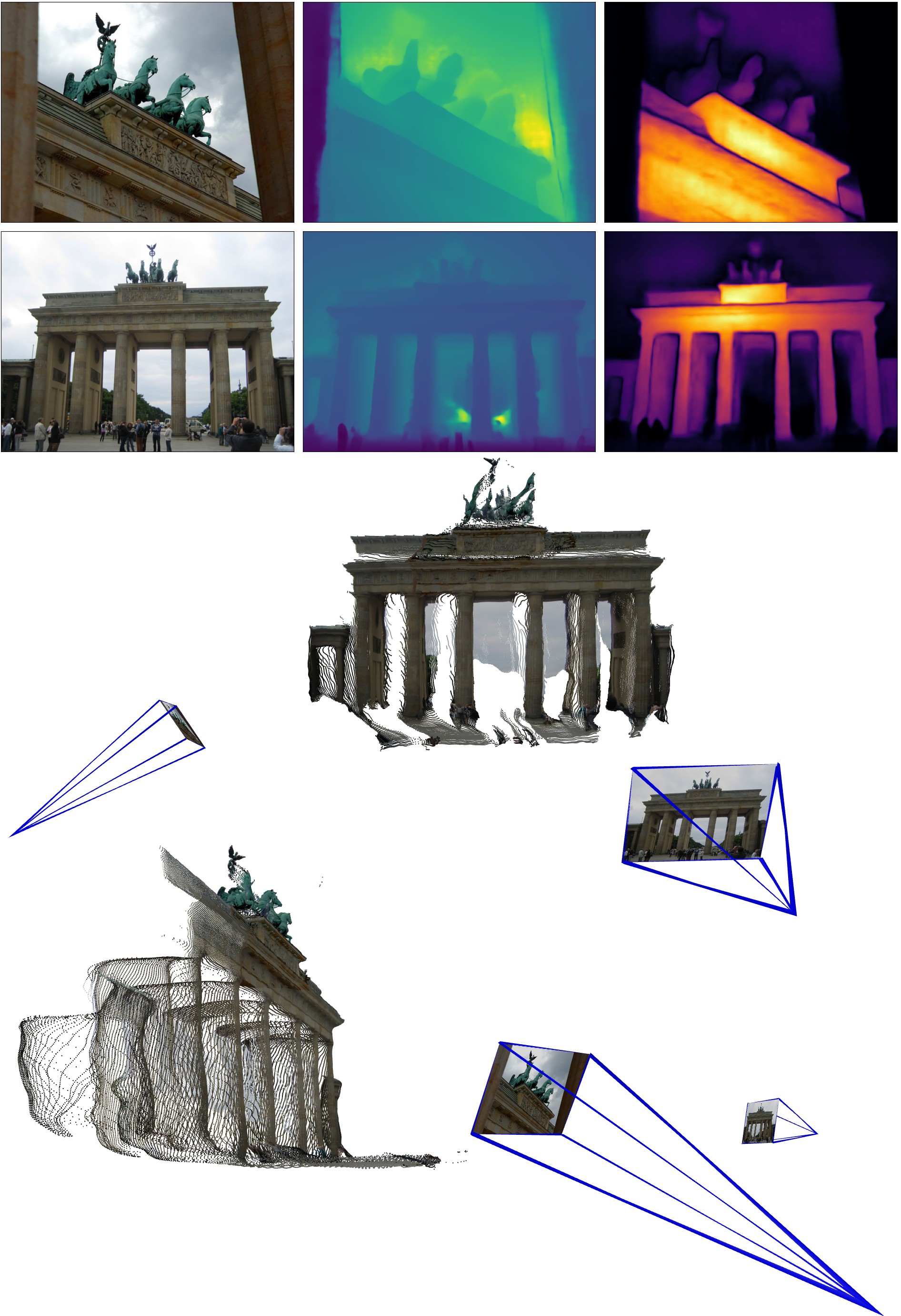
Figure 4: Example of 3D reconstruction of an unseen MegaDepth scene from two images (top-left). Note this is the raw output of the network, i.e. we show the output depthmaps (top-center, see Eq. 8) and confidence maps (top-right), as well as two different viewpoints on the colored pointcloud (middle and bottom). Camera parameters are recovered from the raw pointmaps, see Sec. 3.3 in the main paper. DUSt3R handles strong viewpoint and focal changes without apparent problems

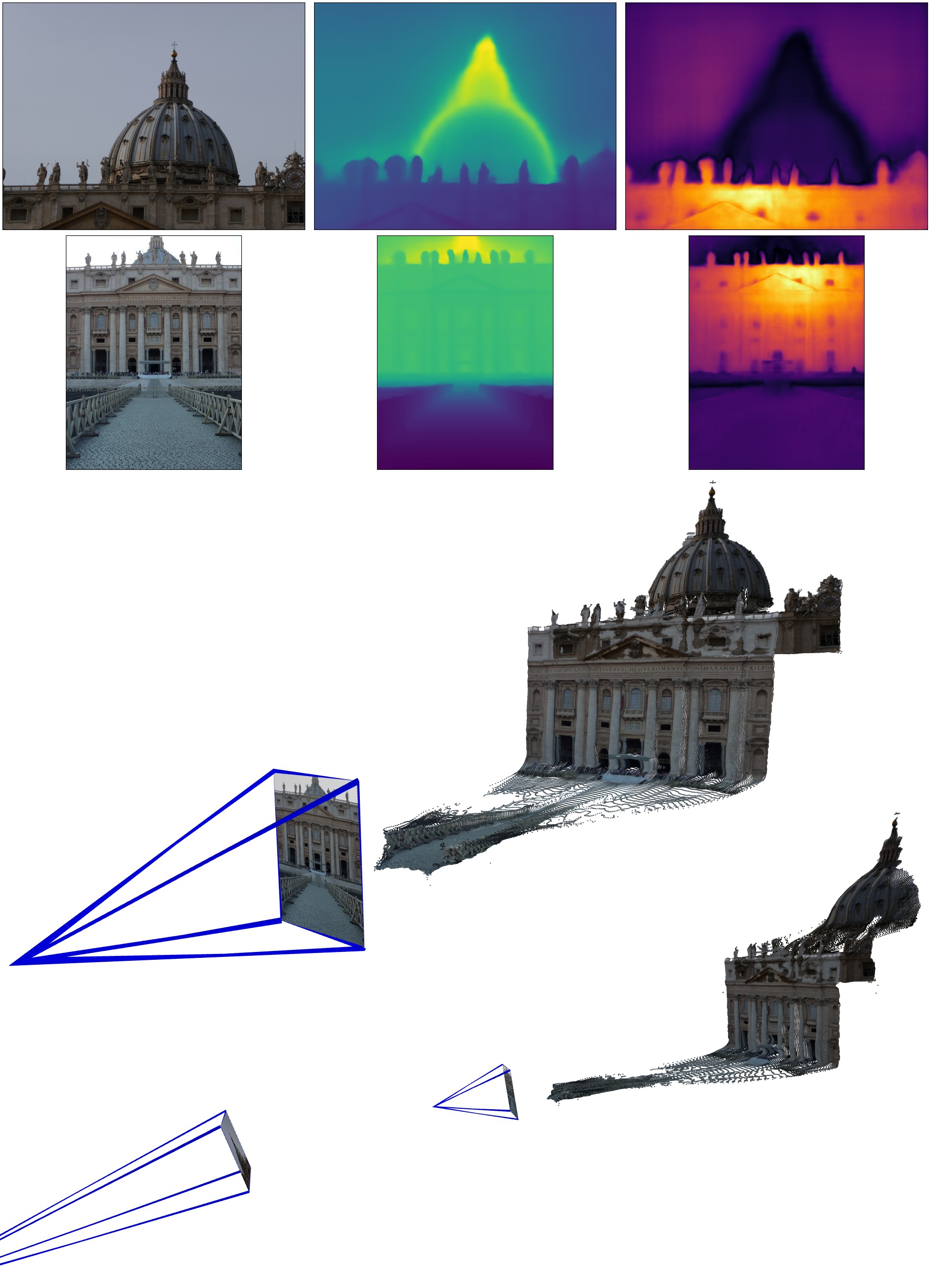
Figure 5: Example of 3D reconstruction of an unseen MegaDepth [55] scene from two images only. Note this is the raw output of the network, i.e. we show the output depthmaps (top-center) and confidence maps (top-right), as well as different viewpoints on the colored pointcloud (middle and bottom). Camera parameters are recovered from the raw pointmaps, see Sec. 3.3 in the main paper. DUSt3R handles strong viewpoint and focal changes without apparent problems

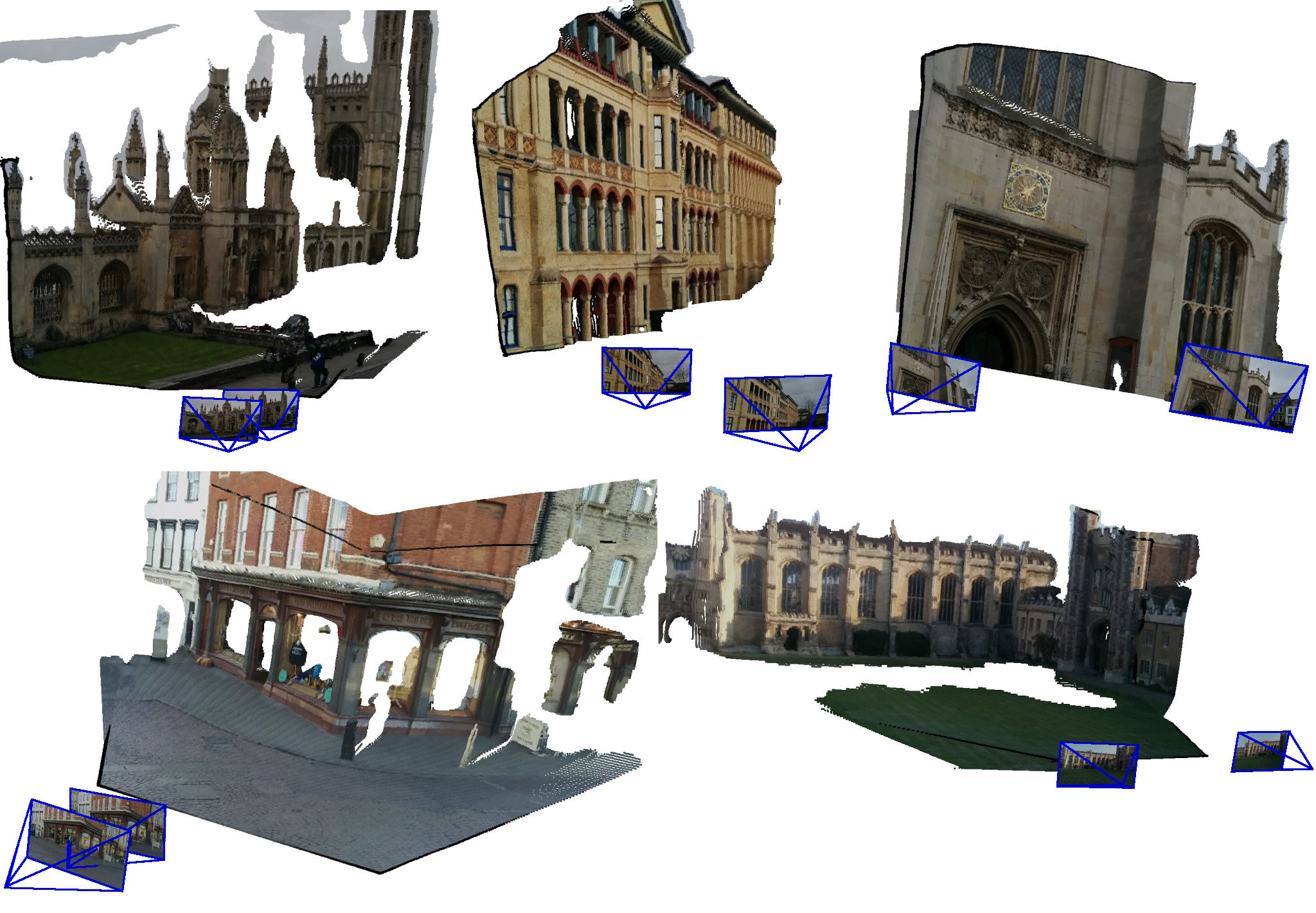
Figure 6: Example of 3D reconstruction from two images only of unseen scenes, namely KingsCollege(Top-Left), OldHospital (Top-Middle), StMarysChurch(Top-Right), ShopFacade(Bottom-Left), GreatCourt(Bottom-Right). Note this is the raw output of the network, i.e. we show new viewpoints on the colored pointclouds. Camera parameters are recovered from the raw pointmaps, see Sec. 3.3 in the main paper.

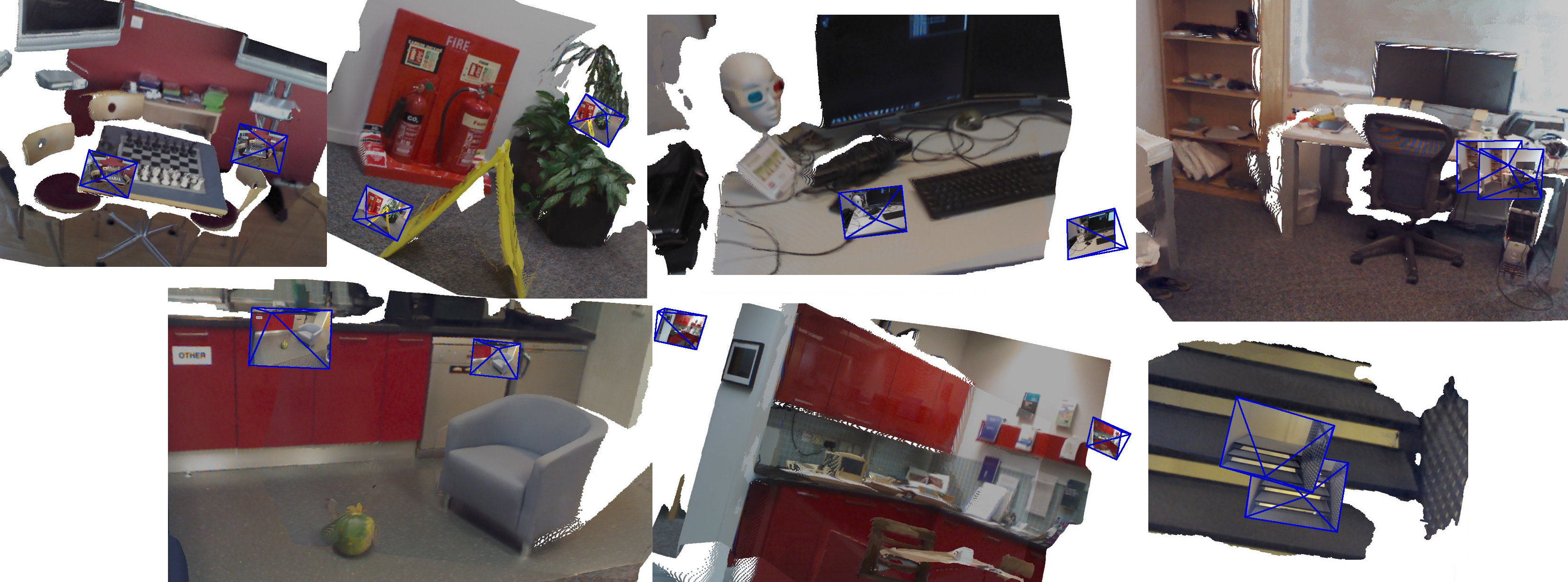
Figure 7: Example of 3D reconstruction from two images only of unseen scenes, namely Chess, Fire, Heads, Office (Top-Row), Pumpkin, Kitchen, Stairs (Bottom-Row). Note this is the raw output of the network, i.e. we show new viewpoints on the colored pointclouds. Camera parameters are recovered from the raw pointmaps, see Sec. 3.3 in the main paper.

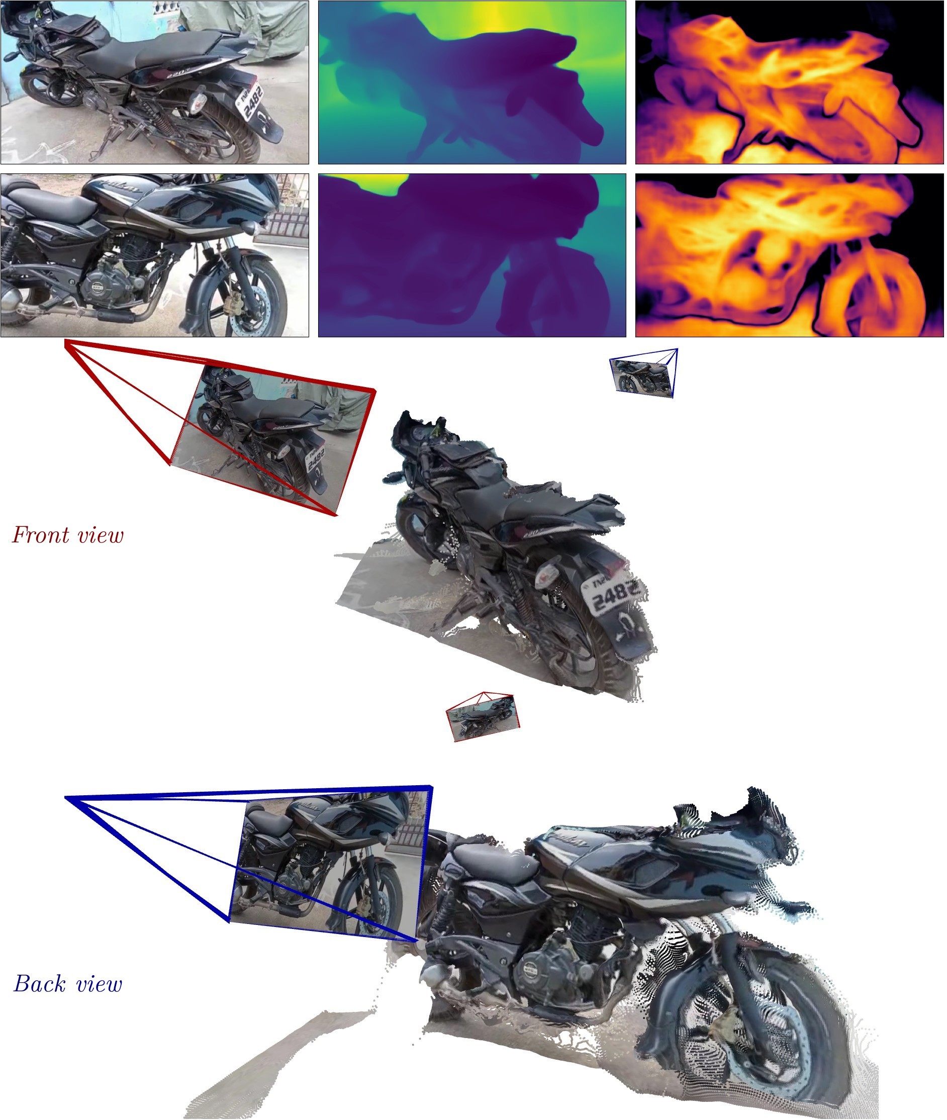
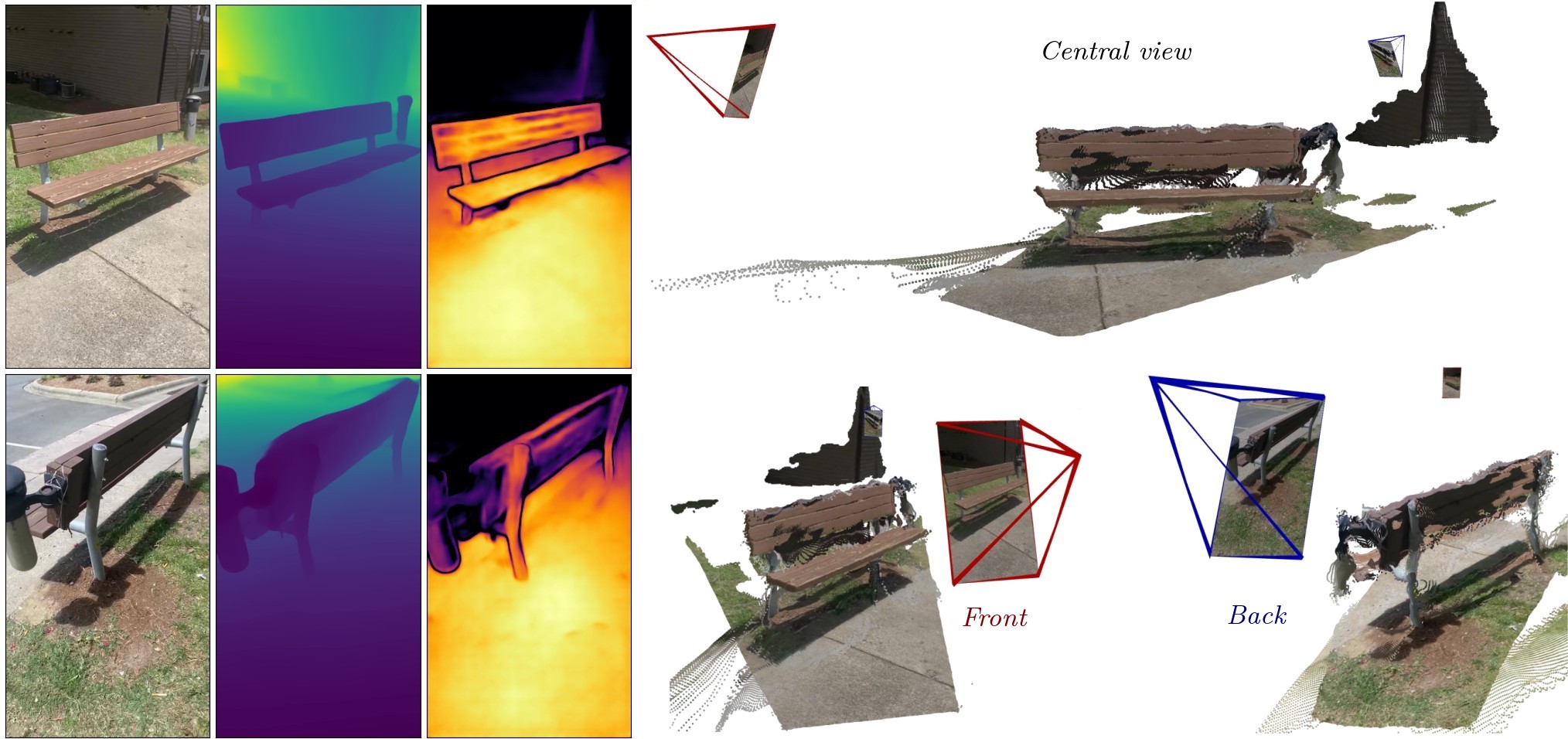
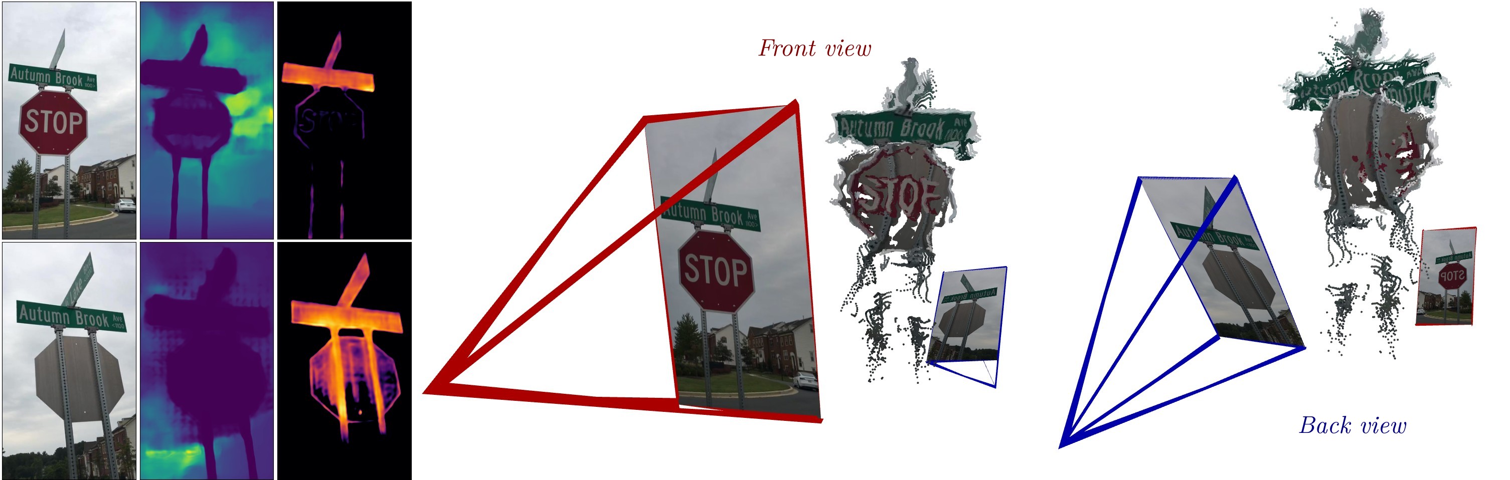
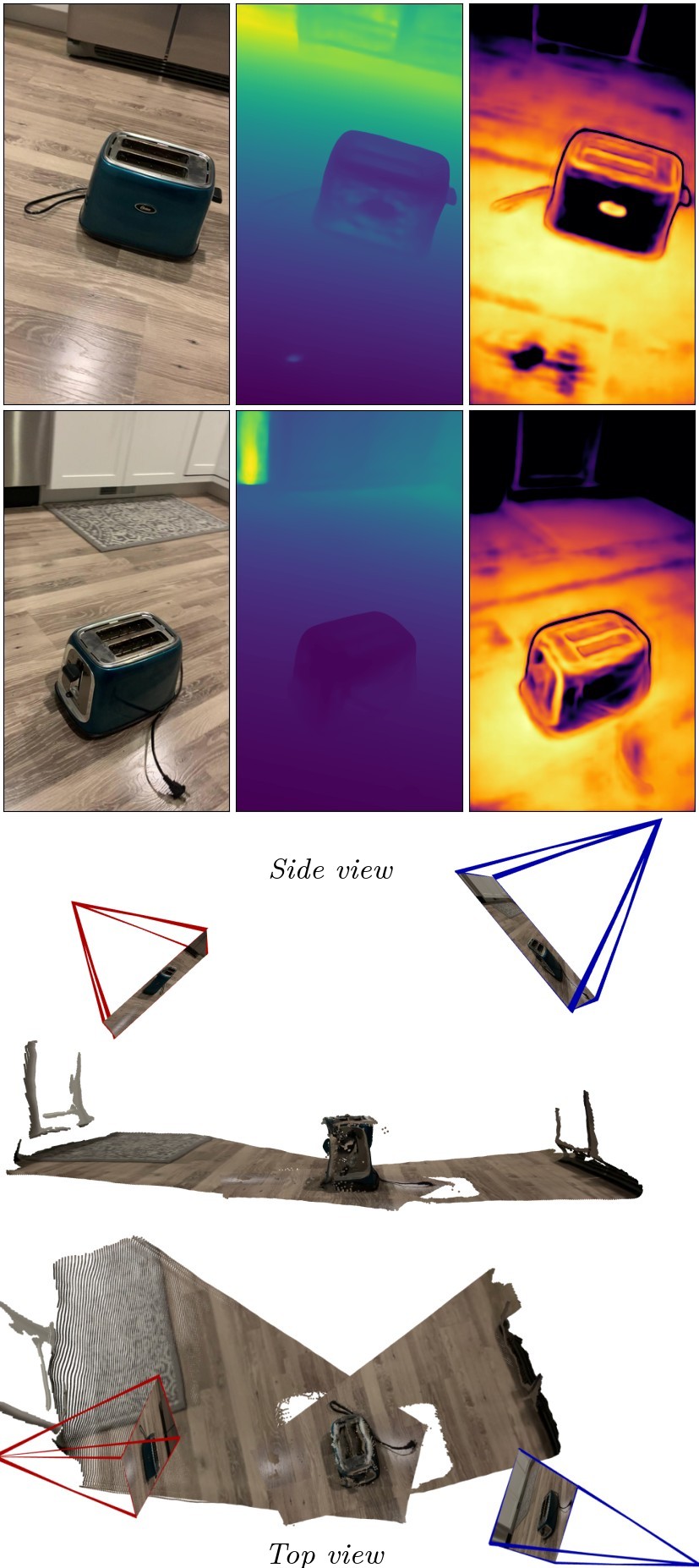
Figure 8: Examples of 3D reconstructions from nearly opposite viewpoints. For each of the 4 cases (motorcycle, toaster, bench, stop sign), we show the two input images (top-left) and the raw output of the network: output depthmaps (top-center) and confidence maps (top-right), as well as two different views on the colored point-clouds (middle and bottom). Camera parameters are recovered from the raw pointmaps, see Sec. 3.3 in the main paper. DUSt3R handles drastic viewpoint changes without apparent issues, even when there is almost no overlapping visual content between images, e.g. for the stop sign and motorcycle. Note that these example cases are not cherry-picked; they are randomly chosen from the set of unseen CO3D_v2 sequences. Please refer to the video for animated visualizations.

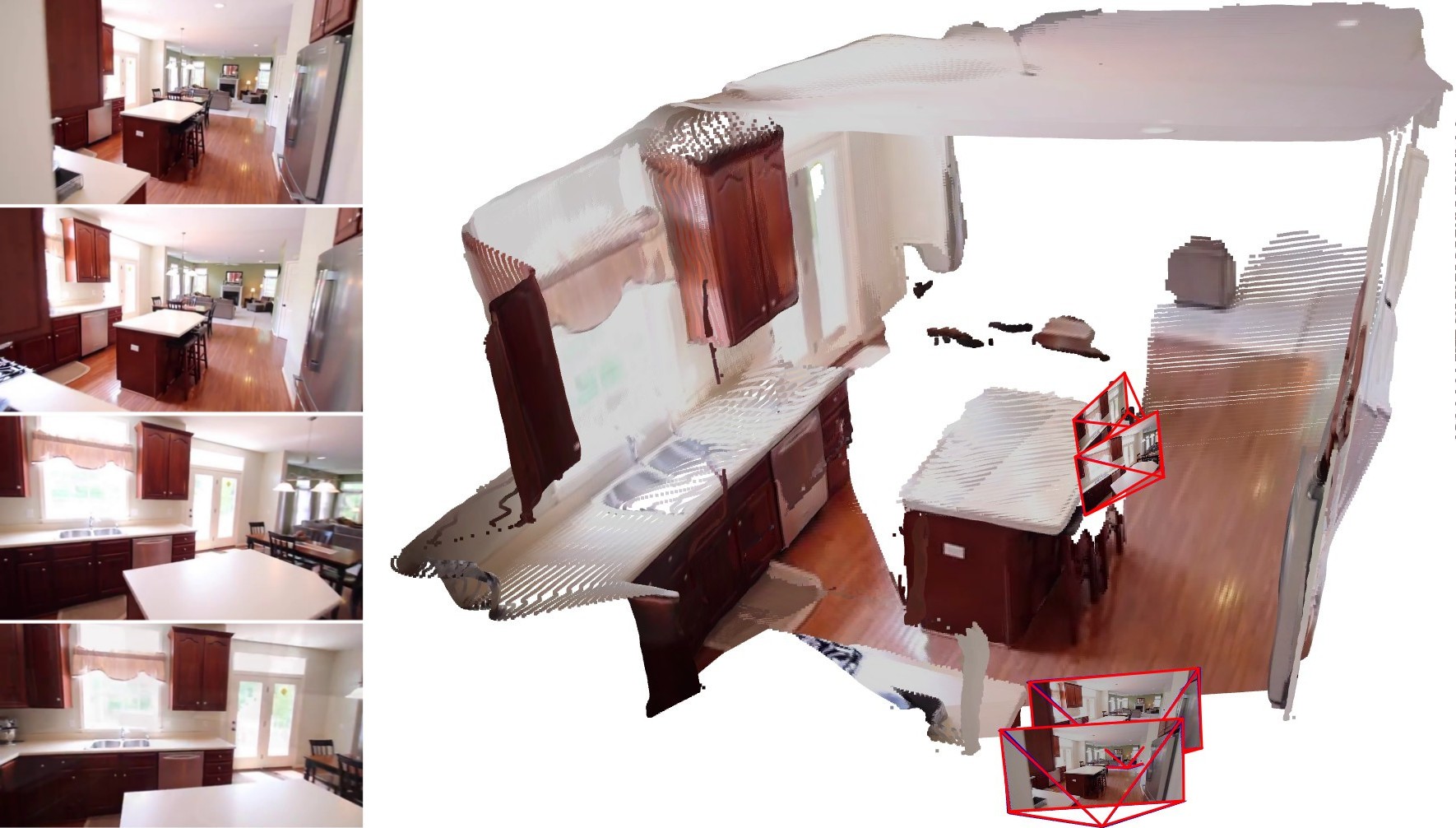
Figure 9: Reconstruction example from 4 random frames of a RealEstate10K indoor sequence, after global alignment. On the left-hand side, we show the 4 input frames, and on the right-hand side the resulting point-cloud and the recovered camera intrinsics and poses.

Appendix

This appendix provides additional details and qualitative results of DUSt3R. We first present in Sec.  qualitative pairwise predictions of the presented architecture on challenging real-life datasets. This section also contains the description of the video accompanying this material. We then propose an extended related works in Sec. , encompassing a wider range of methodological families and geometric vision tasks. Sec.  provides auxiliary ablative results on multi-view pose estimation, that did not fit in the main paper. We then report in Sec.  results on an experimental visual localization task, where the camera intrinsics are unknown. Finally, we details the training and data augmentation procedures in Sec. .

Qualitative results

Point-cloud visualizations.

We present some visualization of DUSt3R’s pairwise results in Figs. 4, 5, 6, 7 and 8. Note these scenes were never seen during training and were not cherry-picked. Also, we did not post-process these results, except for filtering out low-confidence points (based on the output confidence) and removing sky regions for the sake of visualization, i.e. these figures accurately represent the raw output of DUSt3R. Overall, the proposed network is able to perform highly accurate 3D reconstruction from just two images. In Fig. 9, we show the output of DUSt3R after the global alignment stage. In this case, the network has processed all pairs of the 4 input images, and outputs 4 spatially consistent pointmaps along with the corresponding camera parameters.

Note that, for the case of image sequences captured with the same camera, we never enforce the fact that camera intrinsics must be identical for every frame, i.e. all intrinsic parameters are optimized independently. This remains true for all results reported in this appendix and in the main paper, e.g. on multi-view pose estimation with the CO3Dv2 [93] and RealEstate10K [185] datasets.

Supplementary Video. We attach to this appendix a video showcasing the different steps of DUSt3R. In the video, we demonstrate dense 3D reconstruction from a small set of raw RGB images, without using any ground-truth camera parameters (i.e. unknown intrinsic and extrinsic parameters). We show that our method can seamlessly handle monocular predictions, and is able to perform reconstruction and camera pose estimation in extreme binocular cases, where the cameras are facing each other. In addition, we show some qualitative reconstructions of rather large scale scenes from the ETH3D dataset [108].

Extended Related Work

For the sake of exposition, Section 2 of the main paper covered only some (but not all) of the most related works. Because this work covers a large variety of geometric tasks, we complete it in this section with a few equally important topics.

Implicit Camera Models. In our work, we do not explicitly output camera parameters. Likewise, there are several works aiming to express 3D shapes in a canonical space that is not directly related to the input viewpoint. Shapes can be stored as occupancy in regular grids [19, 117, 153, 154, 97, 137, 111], octree structures [127], collections of parametric surface elements [39], point clouds encoders [66, 65, 29], free-form deformation of template meshes [88] or per-view depthmaps [53]. While these approaches arguably perform classification and not actual 3D reconstruction [128], all-in-all, they work only in very constrained setups, usually on ShapeNet [14] and have trouble generalizing to natural scenes with non object-centric views [186]. The question of how to express a complex scene with several object instances in a single canonical frame had yet to be answered: in this work, we also express the reconstruction in a canonical reference frame, but thanks to our scene representation (pointmaps), we still preserve a relationship between image pixels and the 3D space, and we are thus able to perform 3D reconstruction consistently.

Dense Visual SLAM. In visual SLAM, early works on dense 3D reconstruction and ego-motion estimation utilized active depth sensors [73, 183, 135]. Recent works on dense visual SLAM from RGB video stream are able to produce high-quality depth maps and camera trajectories [7, 22, 121, 129, 131, 115], but they inherit the traditional limitations of SLAM, e.g. noisy predictions, drifts and outliers in the pixel correspondences. To make the 3D reconstruction more robust, R3D3 [104] jointly leverages jointly multi-camera constraints and monocular depth cues. Most recently, GO-SLAM [178] proposed real-time global pose optimization by considering the complete history of input frames and continuously aligning all poses that enables instantaneous loop closures and correction of global structure. Still, all SLAM methods assume that the input consists of a sequence of closely related images, e.g. with identical intrinsics, nearby camera poses and small illumination variations. In comparison, our approach handles completely unconstrained image collections.

3D reconstruction from implicit models has undergone significant advancements, largely fueled by the integration of neural networks [71, 147, 80, 172, 60]. Earlier approaches [74, 60, 80] utilize Multi-Layer Perceptron (MLP) to generate continuous surface outputs with only posed RGB images. Innovations like Nerf [71] and its follow-ups  [177, 69, 143, 93, 46, 67] have pioneered density-based volume rendering to represent scenes as continuous 5D functions for both occupancy and color, showing exceptional ability in synthesizing novel views of complex scenes. To handle large-scale scenes, recent approaches  [41, 172, 188, 187] introduce geometry priors to the implicit model, leading to much more detailed reconstructions. In contrast to the implicit 3D reconstruction, our work focuses on the explicit 3D reconstruction and showcases that the proposed DUSt3R can not only have detailed 3D reconstruction but also provide rich geometry for multiple downstream 3D tasks.

RGB-pairs-to-3D takes its roots in two-view geometry [43] and is considered as a stand-alone task or an intermediate step towards the multi-view reconstruction. This process typically involves estimating a dense depth map and determining the relative camera pose from two different views. Recent learning-based approaches formulate this problem either as pose and monocular depth regression [184, 171, 92] or pose and stereo matching [135, 122, 130, 141, 182]. The ultimate goal is to achieve 3D reconstruction from the predicted geometry [2]. In addition to reconstruction tasks, learning from two views also gives an advance in unsupervised pretraining; the recently proposed CroCo [149, 148] introduces a pretext task of cross-view completion from a large set of image pair to learn 3D geometry from unlabeled data and to apply this learned implicit representation to various downstream 3D vision tasks. Our method draws inspiration from the CroCo pipeline, but diverges in its application. Instead of focusing on model pretraining, our approach leverages this pipeline to directly generate 3D pointmaps from the image pair. In this context, the depth map and camera poses are only by-products in our pipeline.

Multi-view Pose Estimation

We include additional results for the multi-view pose estimation task from the main paper (in Sec. 4.2). Namely, we compute the pose accuracy for a smaller number of input images (they are randomly selected from the entire test sequences). Tab. 5 reports our performance and compares with the state of the art. Numbers for state-of-the-art methods are borrowed from the recent PoseDiffusion [139] paper’s tables and plots, hence some numbers are only approximate. Our method consistently outperforms all other methods on the CO3Dv2 dataset by a large margin, even for small number of frames. As can be observed in Fig. 8 and in the attached video, DUSt3R handles opposite viewpoints (i.e. nearly 180^∘ apart) seemingly without much troubles. In the end, DUSt3R obtains relatively stable performance, regardless of the number of input views. When comparing with PoseDiffusion [139] on RealEstate10K, we report performances with and without training on the same dataset. Note that DUSt3R’s training data include a small subset of CO3Dv2 (we used 50 sequences for each category, i.e. less than 7% of the full training set) but no data from RealEstate10K whatsoever.

An example of reconstruction on RealEstate10K is shown in Fig. 9. Our network outputs a consistent pointcloud despite wide baseline viewpoint changes between the first and last pairs of frames.

Methods	N Frames	Co3Dv2 [93]				RealEstate10K [185]
		RRA@15	RTA@15	mAA(30)		mAA(30)
COLMAP+SPSG	3	$\sim$22	$\sim$14	$\sim$15		$\sim$23
PixSfM	3	$\sim$18	$\sim$8	$\sim$10		$\sim$17
Relpose	3	$\sim$56	-	-		-
PoseDiffusion	3	$\sim$75	$\sim$75	$\sim$61		- ($\sim$77)
DUSt3R 512	3	95.3	88.3	77.5		69.5
COLMAP+SPSG	5	$\sim$21	$\sim$17	$\sim$17		$\sim$34
PixSfM	5	$\sim$21	$\sim$16	$\sim$15		$\sim$30
Relpose	5	$\sim$56	-	-		-
PoseDiffusion	5	$\sim$77	$\sim$76	$\sim$63		- ($\sim$78)
DUSt3R 512	5	95.5	86.7	76.5		67.4
COLMAP+SPSG	10	31.6	27.3	25.3		45.2
PixSfM	10	33.7	32.9	30.1		49.4
Relpose	10	57.1	-	-		-
PoseDiffusion	10	80.5	79.8	66.5		48.0 ($\sim$80)
DUSt3R 512	10	96.2	86.8	76.7		67.7

Table 5: Comparison with the state of the art for multi-view pose regression on the CO3Dv2 [93] and RealEstate10K [185] with 3, 5 and 10 random frames. (Parentheses) indicates results obtained after training on RealEstate10K. In contrast, we report results for DUSt3R after global alignment without training on RealEstate10K.

Visual localization

We include additional results of visual localization on the 7-scenes and Cambridge-Landmarks datasets [113, 48]. Namely, we experiment with a scenario where the focal parameter of the querying camera is unknown. In this case, we feed the query image and a database image into DUSt3R, and get an un-scaled 3D reconstruction. We then scale the resulting pointmap according to the ground-truth pointmap of the database image, and extract the pose as described in Sec. 3.3 of the main paper. Tab. 6 shows that this method performs reasonably well on the 7-scenes dataset, where the median translation error is on the order of a few centimeters. On the Cambridge-Landmarks dataset, however, we obtain considerably larger errors. After inspection, we find that the ground-truth database pointmaps are sparse, which prevents any reliable scaling of our reconstruction. On the contrary, 7-scenes provides dense ground-truth pointmaps. We conclude that further work is necessary for ”in-the-wild” visual-localization with unknown intrinsics.

Methods		GT	7Scenes (Indoor) [113]								Cambridge (Outdoor) [48]
		Focals	Chess	Fire	Heads	Office	Pumpkin	Kitchen	Stairs		S. Facade	O. Hospital	K. College	St.Mary’s	G. Court
	DUSt3R 512 from 2D-matching	$\checkmark$	3/0.97	3/0.95	2/1.37	3/1.01	4/1.14	4/1.34	11/2.84		6/0.26	17/0.33	11/0.20	7/0.24	38/0.16
	DUSt3R 512 from scaled rel-pose	$\times$	5/1.08	5/1.18	4/1.33	6/1.05	7/1.25	6/1.37	26/3.56		64/0.97	151/0.88	102/0.88	79/1.46	245/1.08

Table 6: Absolute camera pose on 7Scenes [113] (top 1 image) and Cambridge-Landmarks [48] (top 20 images) datasets. We report the median translation and rotation errors ($cm/^{\circ}$).

Training details

.1 Training data

Ground-truth pointmaps. Ground-truth pointmaps $\bar{X}^{1,1}$ and $\bar{X}^{2,1}$ for images $I^{1}$ and $I^{2}$, respectively, from Eq. (2) in the main paper are obtained from the ground-truth camera intrinsics $K_{1},K_{2}\in\mathbb{R}^{3\times 3}$, camera poses $P_{1},P_{2}\in\mathbb{R}^{3\times 4}$ and depthmaps $D_{1},D_{2}\in\mathbb{R}^{W\times H}$. Specifically, we simply project both pointmaps in the reference frame of $P_{1}$:

$$\bar{X}^{1,1} =K_{1}^{-1}([U;V;\mathbf{1}]\cdot D_{1})$$ (6)

$$\bar{X}^{2,1} =P_{1}P_{2}^{-1}h\left(\bar{X}^{2,2}\right)$$

$$=P_{1}P_{2}^{-1}h\left(K_{2}^{-1}([U;V;\mathbf{1}]\cdot D_{2})\right),$$ (7)

where $X\cdot Y$ denotes element-wise multiplication, $U,V\in\mathbb{R}^{W\times H}$ are the $x,y$ pixel coordinate grids and $h$ is the mapping to homogeneous coordinates, see Eq. (1) of the main paper.

Relation between depthmaps and pointmaps. As a result, the depth value $D^{1}_{i,j}$ at pixel $(i,j)$ in image $I^{1}$ can be recovered as

$$D^{1}_{i,j}=\bar{X}^{1,1}_{i,j,2}.$$ (8)

Therefore, all depthmaps displayed in the main paper and this appendix are straightforwardly extracted from DUSt3R’s output as $X^{1,1}_{:,:,2}$ and $X^{2,2}_{:,:,2}$ for images $I^{1}$ and $I^{2}$, respectively.

Dataset mixture. DUSt3R is trained with a mixture of eight datasets: Habitat [103], ARKitScenes [25], MegaDepth [55], Static Scenes 3D [68], Blended MVS [161], ScanNet++ [165], CO3Dv2 [93] and Waymo [121]. These datasets feature diverse scene types: indoor, outdoor, synthetic, real-world, object-centric, etc. Table 8 shows the number of extracted pairs in each datasets, which amounts to 8.5M in total.

Data augmentation. We use standard data augmentation techniques, namely random color jittering and random center crops, the latter being a form of focal augmentation. Indeed, some datasets are captured using a single or a small number of camera devices, hence many images have practically the same intrinsic parameters. Centered random cropping thus helps in generating more focals. Crops are centered so that the principal point is always centered in the training pairs. At test time, we observe little impact on the results when the principal point is not exactly centered. During training, we also systematically feed each training pair $(I^{1},I^{2})$ as well as its inversion $(I^{2},I^{1})$ to help generalization. Naturally, tokens from these two pairs do not interact.

.2 Training hyperparameters

We report the detailed hyperparameter settings we use for training DUSt3R in Table 7.

Hyperparameters	low-resolution training	high-resolution training	DPT training
Prediction Head	Linear	Linear	DPT[90]
Optimizer	AdamW [61]	AdamW [61]	AdamW [61]
Base learning rate	1e-4	1e-4	1e-4
Weight decay	0.05	0.05	0.05
Adam $\beta$	(0.9, 0.95)	(0.9, 0.95)	(0.9, 0.95)
Pairs per Epoch	700k	70k	70k
Batch size	128	64	64
Epochs	50	100	90
Warmup epochs	10	20	15
Learning rate scheduler	Cosine decay	Cosine decay	Cosine decay
Input resolutions	$224{\times}224$	$512{\times}384$, $512{\times}336$	$512{\times}384$, $512{\times}336$
		$512{\times}288$, $512{\times}256$	$512{\times}288$, $512{\times}256$
		$512{\times}160$	$512{\times}160$
Image Augmentations	Random centered crop, color jitter	Random centered crop, color jitter	Random centered crop, color jitter
Initialization	CroCo v2[148]	low-resolution training	high-resolution training

Table 7: Detailed hyper-parameters for the training, with first a low-resolution training with a linear head followed by a higher-resolution training still with a linear head and a final step of higher-resolution training with a DPT head, in order to save training time

Datasets	Type	N Pairs
Habitat [103]	Indoor / Synthetic	1000k
CO3Dv2 [93]	Object-centric	941k
ScanNet++ [165]	Indoor / Real	224k
ArkitScenes [25]	Indoor / Real	2040k
Static Thing 3D [68]	Object / Synthetic	337k
MegaDepth [55]	Outdoor / Real	1761k
BlendedMVS [161]	Outdoor / Synthetic	1062k
Waymo [121]	Outdoor / Real	1100k

Table 8: Dataset mixture and sample sizes for DUSt3R training.

References

- [1] Henrik Aanæs, Rasmus Ramsbøl Jensen, George Vogiatzis, Engin Tola, and Anders Bjorholm Dahl. Large-scale data for multiple-view stereopsis. IJCV, 2016.
- [2] Samir Agarwala, Linyi Jin, Chris Rockwell, and David F. Fouhey. Planeformers: From sparse view planes to 3d reconstruction. In ECCV, volume 13663 of Lecture Notes in Computer Science, pages 192–209, 2022.
- [3] Daniel Barath, Dmytro Mishkin, Luca Cavalli, Paul-Edouard Sarlin, Petr Hruby, and Marc Pollefeys. Affineglue: Joint matching and robust estimation, 2023.
- [4] Axel Barroso-Laguna, Edgar Riba, Daniel Ponsa, and Krystian Mikolajczyk. Key. net: Keypoint detection by handcrafted and learned cnn filters. In ICCV, pages 5836–5844, 2019.
- [5] Herbert Bay, Tinne Tuytelaars, and Luc Van Gool. Surf: Speeded up robust features. In ECCV, pages 404–417. Springer, 2006.
- [6] Jia-Wang Bian, Huangying Zhan, Naiyan Wang, Tat-Jun Chin, Chunhua Shen, and Ian D. Reid. Auto-rectify network for unsupervised indoor depth estimation. IEEE Trans. Pattern Anal. Mach. Intell., 44(12):9802–9813, 2022.
- [7] Michael Bloesch, Jan Czarnowski, Ronald Clark, Stefan Leutenegger, and Andrew J. Davison. CodeSLAM - learning a compact, optimisable representation for dense visual SLAM. In CVPR, 2018.
- [8] Eric Brachmann, Alexander Krull, Sebastian Nowozin, Jamie Shotton, Frank Michel, Stefan Gumhold, and Carsten Rother. DSAC - differentiable RANSAC for camera localization. In CVPR, 2017.
- [9] Eric Brachmann and Carsten Rother. Learning less is more - 6d camera localization via 3d surface regression. In CVPR, 2018.
- [10] Eric Brachmann and Carsten Rother. Neural-guided RANSAC: learning where to sample model hypotheses. In ICCV, pages 4321–4330. IEEE, 2019.
- [11] Eric Brachmann and Carsten Rother. Visual camera re-localization from RGB and RGB-D images using DSAC. PAMI, 2022.
- [12] Neill D. F. Campbell, George Vogiatzis, Carlos Hernández, and Roberto Cipolla. Using multiple hypotheses to improve depth-maps for multi-view stereo. In ECCV, 2008.
- [13] Carlos Campos, Richard Elvira, Juan J. Gómez Rodríguez, José M. M. Montiel, and Juan D. Tardós. Orb-slam3: An accurate open-source library for visual, visual–inertial, and multimap slam. IEEE Transactions on Robotics, 2021.
- [14] Angel X. Chang, Thomas Funkhouser, Leonidas Guibas, Pat Hanrahan, Qixing Huang, Zimo Li, Silvio Savarese, Manolis Savva, Shuran Song, Hao Su, Jianxiong Xiao, Li Yi, and Fisher Yu. ShapeNet: An Information-Rich 3D Model Repository. Technical Report arXiv:1512.03012 [cs.GR], 2015.
- [15] Devendra Singh Chaplot, Dhiraj Gandhi, Saurabh Gupta, Abhinav Gupta, and Ruslan Salakhutdinov. Learning to explore using active neural slam. arXiv preprint arXiv:2004.05155, 2020.
- [16] Guanying Chen, Kai Han, Boxin Shi, Yasuyuki Matsushita, and Kwan-Yee K. Wong. Deep photometric stereo for non-lambertian surfaces. PAMI, 2022.
- [17] Hongkai Chen, Zixin Luo, Lei Zhou, Yurun Tian, Mingmin Zhen, Tian Fang, David McKinnon, Yanghai Tsin, and Long Quan. Aspanformer: Detector-free image matching with adaptive span transformer. ECCV, 2022.
- [18] Shuo Cheng, Zexiang Xu, Shilin Zhu, Zhuwen Li, Li Erran Li, Ravi Ramamoorthi, and Hao Su. Deep stereo using adaptive thin volume representation with uncertainty awareness. In CVPR, 2020.
- [19] Christopher B Choy, Danfei Xu, JunYoung Gwak, Kevin Chen, and Silvio Savarese. 3D-R2N2: A unified approach for single and multi-view 3d object reconstruction. In ECCV, 2016.
- [20] David Crandall, Andrew Owens, Noah Snavely, and Daniel Huttenlocher. SfM with MRFs: Discrete-continuous optimization for large-scale structure from motion. PAMI, 2013.
- [21] Hainan Cui, Xiang Gao, Shuhan Shen, and Zhanyi Hu. Hsfm: Hybrid structure-from-motion. In Proceedings of the IEEE conference on computer vision and pattern recognition, 2017.
- [22] Jan Czarnowski, Tristan Laidlow, Ronald Clark, and Andrew J. Davison. DeepFactors: Real-time probabilistic dense monocular SLAM. IEEE Robotics Autom. Lett., 5(2):721–728, 2020.
- [23] Angela Dai, Angel X. Chang, Manolis Savva, Maciej Halber, Thomas Funkhouser, and Matthias Nießner. Scannet: Richly-annotated 3d reconstructions of indoor scenes. In CVPR, 2017.
- [24] Amaury Dame, Victor A Prisacariu, Carl Y Ren, and Ian Reid. Dense reconstruction using 3d object shape priors. In CVPR, pages 1288–1295, 2013.
- [25] Afshin Dehghan, Gilad Baruch, Zhuoyuan Chen, Yuri Feigin, Peter Fu, Thomas Gebauer, Daniel Kurz, Tal Dimry, Brandon Joffe, Arik Schwartz, and Elad Shulman. ARKitScenes: A diverse real-world dataset for 3d indoor scene understanding using mobile RGB-D data. In NeurIPS Datasets and Benchmarks, 2021.
- [26] Daniel DeTone, Tomasz Malisiewicz, and Andrew Rabinovich. Superpoint: Self-supervised interest point detection and description. In CVPR Workshops, pages 224–236, 2018.
- [27] Alexey Dosovitskiy, Lucas Beyer, Alexander Kolesnikov, Dirk Weissenborn, Xiaohua Zhai, Thomas Unterthiner, Mostafa Dehghani, Matthias Minderer, Georg Heigold, Sylvain Gelly, Jakob Uszkoreit, and Neil Houlsby. An image is worth 16x16 words: Transformers for image recognition at scale. ICLR, 2021.
- [28] Mihai Dusmanu, Ignacio Rocco, Tomás Pajdla, Marc Pollefeys, Josef Sivic, Akihiko Torii, and Torsten Sattler. D2-net: A trainable CNN for joint description and detection of local features. In CVPR, pages 8092–8101, 2019.
- [29] Haoqiang Fan, Hao Su, and Leonidas J. Guibas. A point set generation network for 3d object reconstruction from a single image. In CVPR, 2017.
- [30] Martin A. Fischler and Robert C. Bolles. Random sample consensus: a paradigm for model fitting with applications to image analysis and automated cartography. Communications of the ACM, 1981.
- [31] Qiancheng Fu, Qingshan Xu, Yew Soon Ong, and Wenbing Tao. Geo-neus: Geometry-consistent neural implicit surfaces learning for multi-view reconstruction. In NeurIPS, 2022.
- [32] Yasutaka Furukawa and Carlos Hernández. Multi-view stereo: A tutorial. Found. Trends Comput. Graph. Vis., 2015.
- [33] Yasutaka Furukawa and Jean Ponce. Accurate, dense, and robust multiview stereopsis. PAMI, 2010.
- [34] Silvano Galliani, Katrin Lasinger, and Konrad Schindler. Massively parallel multiview stereopsis by surface normal diffusion. In ICCV, June 2015.
- [35] Andreas Geiger, Philip Lenz, Christoph Stiller, and Raquel Urtasun. Vision meets robotics: The KITTI dataset. Int. J. Robotics Res., 32(11):1231–1237, 2013.
- [36] Clément Godard, Oisin Mac Aodha, and Gabriel J. Brostow. Unsupervised monocular depth estimation with left-right consistency. In CVPR, 2017.
- [37] Clément Godard, Oisin Mac Aodha, Michael Firman, and Gabriel J. Brostow. Digging into self-supervised monocular depth estimation. In ICCV, pages 3827–3837. IEEE, 2019.
- [38] Leonardo Gomes, Olga Regina Pereira Bellon, and Luciano Silva. 3d reconstruction methods for digital preservation of cultural heritage: A survey. Pattern Recognit. Lett., 2014.
- [39] Thibault Groueix, Matthew Fisher, Vladimir G. Kim, Bryan C. Russell, and Mathieu Aubry. Atlasnet: A papier-mâché approach to learning 3d surface generation. CVPR, 2018.
- [40] Vitor Guizilini, Rares Ambrus, Sudeep Pillai, Allan Raventos, and Adrien Gaidon. 3d packing for self-supervised monocular depth estimation. In CVPR, pages 2482–2491, 2020.
- [41] Haoyu Guo, Sida Peng, Haotong Lin, Qianqian Wang, Guofeng Zhang, Hujun Bao, and Xiaowei Zhou. Neural 3d scene reconstruction with the manhattan-world assumption. In Proceedings of the IEEE/CVF Conference on Computer Vision and Pattern Recognition, pages 5511–5520, 2022.
- [42] Chris Harris, Mike Stephens, et al. A combined corner and edge detector. In Alvey vision conference, volume 15, pages 10–5244. Citeseer, 1988.
- [43] Richard Hartley and Andrew Zisserman. Multiple view geometry in computer vision. Cambridge university press, 2003.
- [44] Richard Hartley and Andrew Zisserman. Multiple View Geometry in Computer Vision. Cambridge University Press, 2004.
- [45] Kaiming He, Xinlei Chen, Saining Xie, Yanghao Li, Piotr Dollár, and Ross B. Girshick. Masked autoencoders are scalable vision learners. In CVPR, 2022.
- [46] Muhammad Zubair Irshad, Sergey Zakharov, Katherine Liu, Vitor Guizilini, Thomas Kollar, Adrien Gaidon, Zsolt Kira, and Rares Ambrus. Neo 360: Neural fields for sparse view synthesis of outdoor scenes. In Proceedings of the IEEE/CVF International Conference on Computer Vision, pages 9187–9198, 2023.
- [47] Nianjuan Jiang, Zhaopeng Cui, and Ping Tan. A global linear method for camera pose registration. In ICCV, 2013.
- [48] Alex Kendall, Matthew Grimes, and Roberto Cipolla. PoseNet: a Convolutional Network for Real-Time 6-DOF Camera Relocalization. In ICCV, 2015.
- [49] Arno Knapitsch, Jaesik Park, Qian-Yi Zhou, and Vladlen Koltun. Tanks and temples: Benchmarking large-scale scene reconstruction. ACM Transactions on Graphics, 36(4), 2017.
- [50] Arno Knapitsch, Jaesik Park, Qian-Yi Zhou, and Vladlen Koltun. Tanks and Temples Online Benchmark. https://www.tanksandtemples.org/leaderboard/, 2017. [Online; accessed 19-October-2023].
- [51] Vincent Lepetit, Francesc Moreno-Noguer, and Pascal Fua. Epnp: An accurate O(n) solution to the pnp problem. IJCV, 2009.
- [52] Vincent Leroy, Jean-Sébastien Franco, and Edmond Boyer. Volume sweeping: Learning photoconsistency for multi-view shape reconstruction. IJCV, 2021.
- [53] Kejie Li, Trung Pham, Huangying Zhan, and Ian D. Reid. Efficient dense point cloud object reconstruction using deformation vector fields. In ECCV, 2018.
- [54] Xiaotian Li, Shuzhe Wang, Yi Zhao, Jakob Verbeek, and Juho Kannala. Hierarchical scene coordinate classification and regression for visual localization. In CVPR, 2020.
- [55] Zhengqi Li and Noah Snavely. Megadepth: Learning single-view depth prediction from internet photos. In CVPR, pages 2041–2050, 2018.
- [56] Chen-Hsuan Lin, Chen Kong, and Simon Lucey. Learning efficient point cloud generation for dense 3d object reconstruction. In AAAI, 2018.
- [57] Chen-Hsuan Lin, Wei-Chiu Ma, Antonio Torralba, and Simon Lucey. BARF: bundle-adjusting neural radiance fields. In ICCV, 2021.
- [58] Philipp Lindenberger, Paul-Edouard Sarlin, Viktor Larsson, and Marc Pollefeys. Pixel-perfect structure-from-motion with featuremetric refinement. In ICCV, 2021.
- [59] Philipp Lindenberger, Paul-Edouard Sarlin, and Marc Pollefeys. Lightglue: Local feature matching at light speed. In ICCV, 2023.
- [60] Shaohui Liu, Yinda Zhang, Songyou Peng, Boxin Shi, Marc Pollefeys, and Zhaopeng Cui. Dist: Rendering deep implicit signed distance function with differentiable sphere tracing. In Proceedings of the IEEE/CVF Conference on Computer Vision and Pattern Recognition, pages 2019–2028, 2020.
- [61] Ilya Loshchilov and Frank Hutter. Decoupled weight decay regularization. In ICLR, 2019.
- [62] David G. Lowe. Distinctive image features from scale-invariant keypoints. IJCV, 2004.
- [63] Bin Luo and Edwin R. Hancock. Procrustes alignment with the EM algorithm. In Computer Analysis of Images and Patterns, CAIP, volume 1689 of Lecture Notes in Computer Science, pages 623–631. Springer, 1999.
- [64] Zeyu Ma, Zachary Teed, and Jia Deng. Multiview stereo with cascaded epipolar raft. In ECCV, 2022.
- [65] Priyanka Mandikal, Navaneet K. L., Mayank Agarwal, and Venkatesh Babu Radhakrishnan. 3d-lmnet: Latent embedding matching for accurate and diverse 3d point cloud reconstruction from a single image. In BMVC, 2018.
- [66] Priyanka Mandikal and Venkatesh Babu Radhakrishnan. Dense 3d point cloud reconstruction using a deep pyramid network. In WACV, 2019.
- [67] Ricardo Martin-Brualla, Noha Radwan, Mehdi SM Sajjadi, Jonathan T Barron, Alexey Dosovitskiy, and Daniel Duckworth. Nerf in the wild: Neural radiance fields for unconstrained photo collections. In Proceedings of the IEEE/CVF Conference on Computer Vision and Pattern Recognition, pages 7210–7219, 2021.
- [68] N. Mayer, E. Ilg, P. Häusser, P. Fischer, D. Cremers, A. Dosovitskiy, and T. Brox. A large dataset to train convolutional networks for disparity, optical flow, and scene flow estimation. In CVPR, 2016.
- [69] Quan Meng, Anpei Chen, Haimin Luo, Minye Wu, Hao Su, Lan Xu, Xuming He, and Jingyi Yu. Gnerf: Gan-based neural radiance field without posed camera. In ICCV, 2021.
- [70] Xiaoxu Meng, Weikai Chen, and Bo Yang. Neat: Learning neural implicit surfaces with arbitrary topologies from multi-view images. In CVPR, 2023.
- [71] Ben Mildenhall, Pratul P. Srinivasan, Matthew Tancik, Jonathan T. Barron, Ravi Ramamoorthi, and Ren Ng. Nerf: Representing scenes as neural radiance fields for view synthesis. In ECCV, 2020.
- [72] Raul Mur-Artal, Jose Maria Martinez Montiel, and Juan D Tardos. Orb-slam: a versatile and accurate monocular slam system. IEEE transactions on robotics, 2015.
- [73] Richard A. Newcombe, Steven Lovegrove, and Andrew J. Davison. DTAM: dense tracking and mapping in real-time. In ICCV, pages 2320–2327, 2011.
- [74] Michael Niemeyer, Lars Mescheder, Michael Oechsle, and Andreas Geiger. Differentiable volumetric rendering: Learning implicit 3d representations without 3d supervision. In Proceedings of the IEEE/CVF Conference on Computer Vision and Pattern Recognition, pages 3504–3515, 2020.
- [75] Michael Niemeyer, Lars M. Mescheder, Michael Oechsle, and Andreas Geiger. Differentiable volumetric rendering: Learning implicit 3d representations without 3d supervision. In CVPR, 2020.
- [76] Michael Oechsle, Songyou Peng, and Andreas Geiger. UNISURF: unifying neural implicit surfaces and radiance fields for multi-view reconstruction. In ICCV, 2021.
- [77] Maxime Oquab, Timothée Darcet, Théo Moutakanni, Huy Vo, Marc Szafraniec, Vasil Khalidov, Pierre Fernandez, Daniel Haziza, Francisco Massa, Alaaeldin El-Nouby, Mahmoud Assran, Nicolas Ballas, Wojciech Galuba, Russell Howes, Po-Yao Huang, Shang-Wen Li, Ishan Misra, Michael G. Rabbat, Vasu Sharma, Gabriel Synnaeve, Hu Xu, Hervé Jégou, Julien Mairal, Patrick Labatut, Armand Joulin, and Piotr Bojanowski. Dinov2: Learning robust visual features without supervision. arXiv preprint arXiv:2304.07193, 2023.
- [78] Onur Özyeşil, Vladislav Voroninski, Ronen Basri, and Amit Singer. A survey of structure from motion*. Acta Numerica, 26:305–364, 2017.
- [79] Emanuele Palazzolo, Jens Behley, Philipp Lottes, Philippe Giguère, and Cyrill Stachniss. Refusion: 3d reconstruction in dynamic environments for RGB-D cameras exploiting residuals. In 2IEEE/RSJ International Conference on Intelligent Robots and Systems (IROS), pages 7855–7862, 2019.
- [80] Jeong Joon Park, Peter Florence, Julian Straub, Richard Newcombe, and Steven Lovegrove. Deepsdf: Learning continuous signed distance functions for shape representation. In The IEEE Conference on Computer Vision and Pattern Recognition (CVPR), June 2019.
- [81] Rémi Pautrat, Iago Suárez, Yifan Yu, Marc Pollefeys, and Viktor Larsson. GlueStick: Robust image matching by sticking points and lines together. In ICCV, 2023.
- [82] Dario Pavllo, Jonas Kohler, Thomas Hofmann, and Aurélien Lucchi. Learning generative models of textured 3d meshes from real-world images. In ICCV, 2021.
- [83] Dario Pavllo, Graham Spinks, Thomas Hofmann, Marie-Francine Moens, and Aurélien Lucchi. Convolutional generation of textured 3d meshes. In NeurIPS, 2020.
- [84] Dario Pavllo, David Joseph Tan, Marie-Julie Rakotosaona, and Federico Tombari. Shape, pose, and appearance from a single image via bootstrapped radiance field inversion. In CVPR, 2023.
- [85] Rui Peng, Rongjie Wang, Zhenyu Wang, Yawen Lai, and Ronggang Wang. Rethinking depth estimation for multi-view stereo: A unified representation. In CVPR, 2022.
- [86] MV Peppa, JP Mills, KD Fieber, I Haynes, S Turner, A Turner, M Douglas, and PG Bryan. Archaeological feature detection from archive aerial photography with a sfm-mvs and image enhancement pipeline. The International Archives of the Photogrammetry, Remote Sensing and Spatial Information Sciences, 42:869–875, 2018.
- [87] Frank Plastria. The Weiszfeld Algorithm: Proof, Amendments, and Extensions, pages 357–389. Springer US, 2011.
- [88] Jhony K. Pontes, Chen Kong, Sridha Sridharan, Simon Lucey, Anders P. Eriksson, and Clinton Fookes. Image2mesh: A learning framework for single image 3d reconstruction. In ACCV, 2018.
- [89] Charles Ruizhongtai Qi, Hao Su, Kaichun Mo, and Leonidas J. Guibas. Pointnet: Deep learning on point sets for 3d classification and segmentation. In CVPR, pages 77–85, 2017.
- [90] René Ranftl, Alexey Bochkovskiy, and Vladlen Koltun. Vision transformers for dense prediction. In ICCV, 2021.
- [91] René Ranftl, Katrin Lasinger, David Hafner, Konrad Schindler, and Vladlen Koltun. Towards robust monocular depth estimation: Mixing datasets for zero-shot cross-dataset transfer. CoRR, 1907.01341/abs, 2020.
- [92] Anurag Ranjan, Varun Jampani, Lukas Balles, Kihwan Kim, Deqing Sun, Jonas Wulff, and Michael J Black. Competitive collaboration: Joint unsupervised learning of depth, camera motion, optical flow and motion segmentation. In Proceedings of the IEEE/CVF conference on computer vision and pattern recognition, pages 12240–12249, 2019.
- [93] Jeremy Reizenstein, Roman Shapovalov, Philipp Henzler, Luca Sbordone, Patrick Labatut, and David Novotný. Common objects in 3d: Large-scale learning and evaluation of real-life 3d category reconstruction. In ICCV, pages 10881–10891, 2021.
- [94] Jerome Revaud, Jon Almazán, Rafael S Rezende, and Cesar Roberto de Souza. Learning with average precision: Training image retrieval with a listwise loss. In ICCV, 2019.
- [95] Jerome Revaud, Yohann Cabon, Romain Brégier, JongMin Lee, and Philippe Weinzaepfel. SACReg: Scene-agnostic coordinate regression for visual localization. CoRR, abs/2307.11702, 2023.
- [96] Jérôme Revaud, César Roberto de Souza, Martin Humenberger, and Philippe Weinzaepfel. R2D2: reliable and repeatable detector and descriptor. In Neurips, pages 12405–12415, 2019.
- [97] Stephan R. Richter and Stefan Roth. Matryoshka networks: Predicting 3d geometry via nested shape layers. In CVPR, 2018.
- [98] Edward Rosten and Tom Drummond. Machine learning for high-speed corner detection. In ECCV. Springer, 2006.
- [99] Paul-Edouard Sarlin, Daniel DeTone, Tomasz Malisiewicz, and Andrew Rabinovich. Superglue: Learning feature matching with graph neural networks. In CVPR, pages 4937–4946, 2020.
- [100] Paul-Edouard Sarlin, Cesar Cadena, Roland Siegwart, and Marcin Dymczyk. From coarse to fine: Robust hierarchical localization at large scale. In CVPR, 2019.
- [101] Paul-Edouard Sarlin, Ajaykumar Unagar, Måns Larsson, Hugo Germain, Carl Toft, Victor Larsson, Marc Pollefeys, Vincent Lepetit, Lars Hammarstrand, Fredrik Kahl, and Torsten Sattler. Back to the Feature: Learning Robust Camera Localization from Pixels to Pose. In CVPR, 2021.
- [102] Torsten Sattler, Bastian Leibe, and Leif Kobbelt. Efficient & effective prioritized matching for large-scale image-based localization. IEEE trans. PAMI, 2017.
- [103] Manolis Savva, Abhishek Kadian, Oleksandr Maksymets, Yili Zhao, Erik Wijmans, Bhavana Jain, Julian Straub, Jia Liu, Vladlen Koltun, Jitendra Malik, Devi Parikh, and Dhruv Batra. Habitat: A platform for embodied ai research. In ICCV, 2019.
- [104] Aron Schmied, Tobias Fischer, Martin Danelljan, Marc Pollefeys, and Fisher Yu. R3D3: dense 3d reconstruction of dynamic scenes from multiple cameras. CoRR, abs/2308.14713, 2023.
- [105] Johannes Lutz Schönberger and Jan-Michael Frahm. Structure-from-motion revisited. In Conference on Computer Vision and Pattern Recognition (CVPR), 2016.
- [106] Johannes Lutz Schönberger, Enliang Zheng, Marc Pollefeys, and Jan-Michael Frahm. Pixelwise view selection for unstructured multi-view stereo. In ECCV, 2016.
- [107] Thomas Schöps, Johannes L. Schönberger, Silvano Galliani, Torsten Sattler, Konrad Schindler, Marc Pollefeys, and Andreas Geiger. ETH3D Online Benchmark. https://www.eth3d.net/high_res_multi_view, 2017. [Online; accessed 19-October-2023].
- [108] Thomas Schöps, Johannes L. Schönberger, Silvano Galliani, Torsten Sattler, Konrad Schindler, Marc Pollefeys, and Andreas Geiger. A multi-view stereo benchmark with high-resolution images and multi-camera videos. In CVPR, 2017.
- [109] Philipp Schröppel, Jan Bechtold, Artemij Amiranashvili, and Thomas Brox. A benchmark and a baseline for robust multi-view depth estimation. In 3DV, pages 637–645, 2022.
- [110] Qi Shan, Brian Curless, Yasutaka Furukawa, Carlos Hernandez, and Steven M Seitz. Occluding contours for multi-view stereo. In CVPR, pages 4002–4009, 2014.
- [111] Zai Shi, Zhao Meng, Yiran Xing, Yunpu Ma, and Roger Wattenhofer. 3d-retr: End-to-end single and multi-view 3d reconstruction with transformers. In BMVC, page 405, 2021.
- [112] Daeyun Shin, Charless C. Fowlkes, and Derek Hoiem. Pixels, voxels, and views: A study of shape representations for single view 3d object shape prediction. In CVPR, 2018.
- [113] Jamie Shotton, Ben Glocker, Christopher Zach, Shahram Izadi, Antonio Criminisi, and Andrew W. Fitzgibbon. Scene coordinate regression forests for camera relocalization in RGB-D images. In CVPR, pages 2930–2937, 2013.
- [114] Nathan Silberman, Derek Hoiem, Pushmeet Kohli, and Rob Fergus. Indoor segmentation and support inference from RGBD images. In ECCV, pages 746–760, 2012.
- [115] Cameron Smith, Yilun Du, Ayush Tewari, and Vincent Sitzmann. Flowcam: Training generalizable 3d radiance fields without camera poses via pixel-aligned scene flow, 2023.
- [116] Jaime Spencer, Chris Russell, Simon Hadfield, and Richard Bowden. Kick back & relax: Learning to reconstruct the world by watching slowtv. In ICCV, 2023.
- [117] Riccardo Spezialetti, David Joseph Tan, Alessio Tonioni, Keisuke Tateno, and Federico Tombari. A divide et impera approach for 3d shape reconstruction from multiple views. In 3DV, 2020.
- [118] Jürgen Sturm, Nikolas Engelhard, Felix Endres, Wolfram Burgard, and Daniel Cremers. A benchmark for the evaluation of RGB-D SLAM systems. In IEEE/RSJ International Conference on Intelligent Robots and Systems (IROS), pages 573–580. IEEE, 2012.
- [119] Jiaming Sun, Zehong Shen, Yuang Wang, Hujun Bao, and Xiaowei Zhou. LoFTR: Detector-free local feature matching with transformers. CVPR, 2021.
- [120] Libo Sun, Jia-Wang Bian, Huangying Zhan, Wei Yin, Ian Reid, and Chunhua Shen. Sc-depthv3: Robust self-supervised monocular depth estimation for dynamic scenes. CoRR, 2211.03660, 2022.
- [121] Pei Sun, Henrik Kretzschmar, Xerxes Dotiwalla, Aurelien Chouard, Vijaysai Patnaik, Paul Tsui, James Guo, Yin Zhou, Yuning Chai, Benjamin Caine, Vijay Vasudevan, Wei Han, Jiquan Ngiam, Hang Zhao, Aleksei Timofeev, Scott Ettinger, Maxim Krivokon, Amy Gao, Aditya Joshi, Yu Zhang, Jonathon Shlens, Zhifeng Chen, and Dragomir Anguelov. Scalability in perception for autonomous driving: Waymo open dataset. In CVPR, June 2020.
- [122] Chengzhou Tang and Ping Tan. Ba-net: Dense bundle adjustment network. Proceedings of the International Conference on Learning Representations, 2018.
- [123] Shitao Tang, Chengzhou Tang, Rui Huang, Siyu Zhu, and Ping Tan. Learning camera localization via dense scene matching. In CVPR, 2021.
- [124] Shitao Tang, Sicong Tang, Andrea Tagliasacchi, Ping Tan, and Yasutaka Furukawa. Neumap: Neural coordinate mapping by auto-transdecoder for camera localization. In CVPR, 2023.
- [125] Shitao Tang, Jiahui Zhang, Siyu Zhu, and Ping Tan. Quadtree attention for vision transformers. ICLR, 2022.
- [126] Maxim Tatarchenko, Alexey Dosovitskiy, and Thomas Brox. Multi-view 3d models from single images with a convolutional network. In ECCV, 2016.
- [127] Maxim Tatarchenko, Alexey Dosovitskiy, and Thomas Brox. Octree generating networks: Efficient convolutional architectures for high-resolution 3d outputs. In ICCV, 2017.
- [128] Maxim Tatarchenko, Stephan R. Richter, René Ranftl, Zhuwen Li, Vladlen Koltun, and Thomas Brox. What do single-view 3d reconstruction networks learn? In CVPR, 2019.
- [129] Keisuke Tateno, Federico Tombari, Iro Laina, and Nassir Navab. CNN-SLAM: real-time dense monocular SLAM with learned depth prediction. In CVPR, 2017.
- [130] Zachary Teed and Jia Deng. Deepv2d: Video to depth with differentiable structure from motion. In ICLR, 2020.
- [131] Zachary Teed and Jia Deng. DROID-SLAM: deep visual SLAM for monocular, stereo, and RGB-D cameras. In NeurIPS, pages 16558–16569, 2021.
- [132] Sebastian Thrun. Probabilistic robotics. Communications of the ACM, 45(3):52–57, 2002.
- [133] Engin Tola, Christoph Strecha, and Pascal Fua. Efficient large-scale multi-view stereo for ultra high-resolution image sets. Mach. Vis. Appl., 2012.
- [134] Michał Tyszkiewicz, Pascal Fua, and Eduard Trulls. Disk: Learning local features with policy gradient. Advances in Neural Information Processing Systems, 33:14254–14265, 2020.
- [135] Benjamin Ummenhofer, Huizhong Zhou, Jonas Uhrig, Nikolaus Mayer, Eddy Ilg, Alexey Dosovitskiy, and Thomas Brox. DeMoN: Depth and motion network for learning monocular stereo. In CVPR, pages 5622–5631, 2017.
- [136] Sheng Wan, Tung-Yu Wu, Wing H. Wong, and Chen-Yi Lee. Confnet: Predict with confidence. In IEEE Intern. Conf.on Acoustics, Speech and Signal Processing (ICASSP), pages 2921–2925, 2018.
- [137] Dan Wang, Xinrui Cui, Xun Chen, Zhengxia Zou, Tianyang Shi, Septimiu Salcudean, Z. Jane Wang, and Rabab Ward. Multi-view 3d reconstruction with transformers. In ICCV, pages 5702–5711, 2021.
- [138] Fangjinhua Wang, Silvano Galliani, Christoph Vogel, Pablo Speciale, and Marc Pollefeys. Patchmatchnet: Learned multi-view patchmatch stereo. In CVPR, pages 14194–14203, 2021.
- [139] Jianyuan Wang, Christian Rupprecht, and David Novotný. Posediffusion: Solving pose estimation via diffusion-aided bundle adjustment. In ICCV, 2023.
- [140] Jinglu Wang, Bo Sun, and Yan Lu. Mvpnet: Multi-view point regression networks for 3d object reconstruction from A single image. In AAAI, 2019.
- [141] Jianyuan Wang, Yiran Zhong, Yuchao Dai, Stan Birchfield, Kaihao Zhang, Nikolai Smolyanskiy, and Hongdong Li. Deep two-view structure-from-motion revisited. In Proceedings of the IEEE/CVF conference on Computer Vision and Pattern Recognition, pages 8953–8962, 2021.
- [142] Peng Wang, Lingjie Liu, Yuan Liu, Christian Theobalt, Taku Komura, and Wenping Wang. Neus: Learning neural implicit surfaces by volume rendering for multi-view reconstruction. In NeurIPS, 2021.
- [143] Peng Wang, Lingjie Liu, Yuan Liu, Christian Theobalt, Taku Komura, and Wenping Wang. Neus: Learning neural implicit surfaces by volume rendering for multi-view reconstruction. NeurIPS, 2021.
- [144] Shuzhe Wang, Juho Kannala, Marc Pollefeys, and Daniel Barath. Guiding local feature matching with surface curvature. In Proceedings of the IEEE/CVF International Conference on Computer Vision (ICCV), pages 17981–17991, October 2023.
- [145] Yiqun Wang, Ivan Skorokhodov, and Peter Wonka. Hf-neus: Improved surface reconstruction using high-frequency details. In NeurIPS, 2022.
- [146] Yuesong Wang, Zhaojie Zeng, Tao Guan, Wei Yang, Zhuo Chen, Wenkai Liu, Luoyuan Xu, and Yawei Luo. Adaptive patch deformation for textureless-resilient multi-view stereo. In CVPR, 2023.
- [147] Yi Wei, Shaohui Liu, Yongming Rao, Wang Zhao, Jiwen Lu, and Jie Zhou. Nerfingmvs: Guided optimization of neural radiance fields for indoor multi-view stereo. In ICCV, 2021.
- [148] Philippe Weinzaepfel, Thomas Lucas, Vincent Leroy, Yohann Cabon, Vaibhav Arora, Romain Brégier, Gabriela Csurka, Leonid Antsfeld, Boris Chidlovskii, and Jérôme Revaud. CroCo v2: Improved Cross-view Completion Pre-training for Stereo Matching and Optical Flow. In ICCV, 2023.
- [149] Weinzaepfel, Philippe and Leroy, Vincent and Lucas, Thomas and Brégier, Romain and Cabon, Yohann and Arora, Vaibhav and Antsfeld, Leonid and Chidlovskii, Boris and Csurka, Gabriela and Revaud Jérôme. CroCo: Self-Supervised Pre-training for 3D Vision Tasks by Cross-View Completion. In NeurIPS, 2022.
- [150] Olivia Wiles, Georgia Gkioxari, Richard Szeliski, and Justin Johnson. Synsin: End-to-end view synthesis from a single image. In CVPR, 2020.
- [151] Xin Wu, Hao Zhao, Shunkai Li, Yingdian Cao, and Hongbin Zha. Sc-wls: Towards interpretable feed-forward camera re-localization. In ECCV, 2022.
- [152] Yuxi Xiao, Nan Xue, Tianfu Wu, and Gui-Song Xia. Level-S2fM: Structure From Motion on Neural Level Set of Implicit Surfaces. In Proceedings of the IEEE/CVF Conference on Computer Vision and Pattern Recognition, 2023.
- [153] Haozhe Xie, Hongxun Yao, Xiaoshuai Sun, Shangchen Zhou, and Shengping Zhang. Pix2vox: Context-aware 3d reconstruction from single and multi-view images. In ICCV, 2019.
- [154] Haozhe Xie, Hongxun Yao, Shengping Zhang, Shangchen Zhou, and Wenxiu Sun. Pix2vox++: Multi-scale context-aware 3d object reconstruction from single and multiple images. IJCV, 2020.
- [155] Guangkai Xu, Wei Yin, Hao Chen, Chunhua Shen, Kai Cheng, and Feng Zhao. Frozenrecon: Pose-free 3d scene reconstruction with frozen depth models. In ICCV, 2023.
- [156] Qingshan Xu and Wenbing Tao. Learning inverse depth regression for multi-view stereo with correlation cost volume. In AAAI, 2020.
- [157] Jiayu Yang, Wei Mao, José M. Álvarez, and Miaomiao Liu. Cost volume pyramid based depth inference for multi-view stereo. In CVPR, pages 4876–4885, 2020.
- [158] Luwei Yang, Ziqian Bai, Chengzhou Tang, Honghua Li, Yasutaka Furukawa, and Ping Tan. Sanet: Scene agnostic network for camera localization. In ICCV, 2019.
- [159] Zhenpei Yang, Zhile Ren, Qi Shan, and Qixing Huang. MVS2D: efficient multiview stereo via attention-driven 2d convolutions. In CVPR, pages 8564–8574, 2022.
- [160] Yao Yao, Zixin Luo, Shiwei Li, Tian Fang, and Long Quan. Mvsnet: Depth inference for unstructured multi-view stereo. In ECCV, 2018.
- [161] Yao Yao, Zixin Luo, Shiwei Li, Jingyang Zhang, Yufan Ren, Lei Zhou, Tian Fang, and Long Quan. Blendedmvs: A large-scale dataset for generalized multi-view stereo networks. In CVPR, pages 1787–1796, 2020.
- [162] Lior Yariv, Yoni Kasten, Dror Moran, Meirav Galun, Matan Atzmon, Ronen Basri, and Yaron Lipman. Multiview neural surface reconstruction by disentangling geometry and appearance. In NeurIPS, 2020.
- [163] Xinyi Ye, Weiyue Zhao, Tianqi Liu, Zihao Huang, Zhiguo Cao, and Xin Li. Constraining depth map geometry for multi-view stereo: A dual-depth approach with saddle-shaped depth cells. ICCV, 2023.
- [164] Zhichao Ye, Chong Bao, Xin Zhou, Haomin Liu, Hujun Bao, and Guofeng Zhang. Ec-sfm: Efficient covisibility-based structure-from-motion for both sequential and unordered images. CoRR, abs/2302.10544, 2023.
- [165] Chandan Yeshwanth, Yueh-Cheng Liu, Matthias Nießner, and Angela Dai. Scannet++: A high-fidelity dataset of 3d indoor scenes. In Proceedings of the International Conference on Computer Vision (ICCV), 2023.
- [166] Kwang Moo Yi, Eduard Trulls, Vincent Lepetit, and Pascal Fua. Lift: Learned invariant feature transform. In Computer Vision–ECCV 2016: 14th European Conference, Amsterdam, The Netherlands, October 11-14, 2016, Proceedings, Part VI 14, pages 467–483. Springer, 2016.
- [167] Wei Yin, Chi Zhang, Hao Chen, Zhipeng Cai, Gang Yu, Kaixuan Wang, Xiaozhi Chen, and Chunhua Shen. Metric3d: Towards zero-shot metric 3d prediction from a single image. In ICCV, 2023.
- [168] Wei Yin, Jianming Zhang, Oliver Wang, Simon Niklaus, Simon Chen, Yifan Liu, and Chunhua Shen. Towards accurate reconstruction of 3d scene shape from a single monocular image, 2022.
- [169] Wei Yin, Jianming Zhang, Oliver Wang, Simon Niklaus, Simon Chen, Yifan Liu, and Chunhua Shen. Towards accurate reconstruction of 3d scene shape from a single monocular image. IEEE Transactions on Pattern Analysis and Machine Intelligence (TPAMI), 2022.
- [170] Wei Yin, Jianming Zhang, Oliver Wang, Simon Niklaus, Long Mai, Simon Chen, and Chunhua Shen. Learning to recover 3d scene shape from a single image. In CVPR, 2020.
- [171] Zhichao Yin and Jianping Shi. Geonet: Unsupervised learning of dense depth, optical flow and camera pose. In Proceedings of the IEEE conference on computer vision and pattern recognition, pages 1983–1992, 2018.
- [172] Zehao Yu, Songyou Peng, Michael Niemeyer, Torsten Sattler, and Andreas Geiger. Monosdf: Exploring monocular geometric cues for neural implicit surface reconstruction. Advances in neural information processing systems, 35:25018–25032, 2022.
- [173] Weihao Yuan, Xiaodong Gu, Zuozhuo Dai, Siyu Zhu, and Ping Tan. Neural window fully-connected crfs for monocular depth estimation. In CVPR, pages 3906–3915, 2022.
- [174] Zhaojie Zeng. OpenMVS. https://github.com/cdcseacave/openMVS, 2015. [Online; accessed 19-October-2023].
- [175] Jingyang Zhang, Shiwei Li, Zixin Luo, Tian Fang, and Yao Yao. Vis-mvsnet: Visibility-aware multi-view stereo network. Int. J. Comput. Vis., 131(1):199–214, 2023.
- [176] Jason Y. Zhang, Deva Ramanan, and Shubham Tulsiani. Relpose: Predicting probabilistic relative rotation for single objects in the wild. In Shai Avidan, Gabriel J. Brostow, Moustapha Cissé, Giovanni Maria Farinella, and Tal Hassner, editors, ECCV, pages 592–611, 2022.
- [177] Kai Zhang, Gernot Riegler, Noah Snavely, and Vladlen Koltun. Nerf++: Analyzing and improving neural radiance fields. arXiv preprint arXiv:2010.07492, 2020.
- [178] Youmin Zhang, Fabio Tosi, Stefano Mattoccia, and Matteo Poggi. GO-SLAM: Global optimization for consistent 3d instant reconstruction. In ICCV, pages 3727–3737, October 2023.
- [179] Zhe Zhang, Rui Peng, Yuxi Hu, and Ronggang Wang. Geomvsnet: Learning multi-view stereo with geometry perception. In CVPR, 2023.
- [180] Chen Zhao, Yixiao Ge, Feng Zhu, Rui Zhao, Hongsheng Li, and Mathieu Salzmann. Progressive correspondence pruning by consensus learning. In ICCV, 2021.
- [181] Chaoqiang Zhao, Youmin Zhang, Matteo Poggi, Fabio Tosi, Xianda Guo, Zheng Zhu, Guan Huang, Yang Tang, and Stefano Mattoccia. MonoViT: Self-supervised monocular depth estimation with a vision transformer. In International Conference on 3D Vision (3DV), sep 2022.
- [182] Yunhan Zhao, Connelly Barnes, Yuqian Zhou, Eli Shechtman, Sohrab Amirghodsi, and Charless C. Fowlkes. Geofill: Reference-based image inpainting with better geometric understanding. In WACV, pages 1776–1786, 2023.
- [183] Huizhong Zhou, Benjamin Ummenhofer, and Thomas Brox. DeepTAM: Deep tracking and mapping with convolutional neural networks. Int. J. Comput. Vis., 128(3):756–769, 2020.
- [184] Tinghui Zhou, Matthew Brown, Noah Snavely, and David G Lowe. Unsupervised learning of depth and ego-motion from video. In Proceedings of the IEEE conference on computer vision and pattern recognition, pages 1851–1858, 2017.
- [185] Tinghui Zhou, Richard Tucker, John Flynn, Graham Fyffe, and Noah Snavely. Stereo magnification: Learning view synthesis using multiplane images. ACM Trans. Graph. (Proc. SIGGRAPH), 37, 2018.
- [186] Rui Zhu, Chaoyang Wang, Chen-Hsuan Lin, Ziyan Wang, and Simon Lucey. Semantic photometric bundle adjustment on natural sequences. CoRR, 2017.
- [187] Zihan Zhu, Songyou Peng, Viktor Larsson, Zhaopeng Cui, Martin R Oswald, Andreas Geiger, and Marc Pollefeys. Nicer-slam: Neural implicit scene encoding for rgb slam. arXiv preprint arXiv:2302.03594, 2023.
- [188] Zihan Zhu, Songyou Peng, Viktor Larsson, Weiwei Xu, Hujun Bao, Zhaopeng Cui, Martin R Oswald, and Marc Pollefeys. Nice-slam: Neural implicit scalable encoding for slam. In Proceedings of the IEEE/CVF Conference on Computer Vision and Pattern Recognition, pages 12786–12796, 2022.