Adaptation using spatially distributed Gaussian Processes

Abstract

We consider the accuracy of an approximate posterior distribution in nonparametric regression problems by combining posterior distributions computed on subsets of the data defined by the locations of the independent variables. We show that this approximate posterior retains the rate of recovery of the full data posterior distribution, where the rate of recovery adapts to the smoothness of the true regression function. As particular examples we consider Gaussian process priors based on integrated Brownian motion and the Matérn kernel augmented with a prior on the length scale. Besides theoretical guarantees we present a numerical study of the methods both on synthetic and real world data. We also propose a new aggregation technique, which numerically outperforms previous approaches.

1 Introduction

Gaussian processes (GPs) are standard tools in statistical and machine learning. They provide a particularly effective prior distribution over the space of functions and are routinely used in regression and classification tasks, amongst others. The monograph rasmussen:williams:2006 gives an in-depth overview of the foundations and practical applications of this approach. However, GPs scale poorly with the sample size $n$. For instance, in regression the computational complexity and memory requirements are of the orders $O(n^{3})$ and $O(n^{2})$, respectively. This limitation has triggered the development of various approximation methods, including sparse approximations of the empirical covariance matrices gibbs:poole:stockmeyer:1976 ; saad:1990 ; quinonero:rasmussen:2005 , variational Bayes approximations titsias:2009 ; burt2019 ; nieman2022 or distributed methods. We focus on the latter method in this paper.

In distributed (or divide-and-conquer) methods, the computational burden is reduced by splitting the data over “local” machines (or servers, experts or cores). Next the computations are carried out locally, in parallel to each other, before transmitting the outcomes to a “central” server or core, where the partial, local results are combined, forming the final outcome of the procedure. This distributed architecture occurs naturally when data is collected and processed locally and only a summary statistic is transmitted to a central server. Besides speeding up the computations and reducing the memory requirements, distributed methods can also help in protecting privacy, as the data do not have to be stored in a central data base, but are processed locally.

In the literature various distributed methods were proposed to speed up Bayesian computation, in particular in the context of Gaussian Processes. One can distinguish two main strategies depending on the data-splitting technique. The first approach is to partition the data randomly over the servers, computing a posterior distribution on each server and finally aggregating these local distributions by some type of averaging. Examples include Consensus Monte Carlo scott:blocker:et.al:16 , WASP srivastava:2015a , Generalized Product of Experts cao:fleet:14 , Bayesian Committee Machine tresp:2000 ; deisenroth2015 , Distributed Bayesian Varying Coefficients guhaniyogi2022distributed and Distributed Kriging guhaniyogi2017divide . The second approach takes advantage of the spatial structure of the data and splits the observations based on a partition of the design space. Each machine is assigned a specific region of the space, a local posterior distribution is computed using the data in this region, and these are glued together to form the final answer. This approach is referred to as the Naive-Local-Experts model, see kim:mallick:holmes ; vasudevan2009gaussian . We discuss various methods of combining the local outputs in Section 4.2, including a new proposal, which outperforms its competitors in the case that the length scale of the priors is determined from the data.

A number of papers in the literature studied the randomly split data approach, deriving theoretical guarantees, but also limitations, for a range of methods and models. Under the assumption that the regularity of the underlying functional parameter is known, minimax rate-optimal contraction rates and frequentist coverage guarantees for Bayesian credible sets were derived in the context of the Gaussian white noise szabo:vzanten:19 and nonparametric regression models guhaniyogi2017divide ; shang:cheng:2015 ; hadji2022optimal . However, in practice the latter regularity is typically not known, but inferred from the data in some way. In the mentioned references it is shown that with randomly split data, standard adaptation techniques necessarily lead to highly sub-optimal inference, see szabo:vzanten:19 . In the numerical analysis in the present paper we observe this on both synthetic and real world data sets.

In contrast, spatially partitioned distributed approaches have received little theoretical attention, despite their popularity in applications. In this paper we aim to fill this gap in the literature. We derive general contraction rate theorems under mild assumptions and apply them in the context of the nonparametric regression and classification models. We also consider two specific GP priors: the rescaled integrated Brownian motion and the Matérn process and show that both priors (augmented with an additional layer of prior on the scale parameter) lead to rate-adaptive posterior contraction rates. This is in sharp contrast to the randomly split data framework, which necessarily results in sub-optimal estimation. Thus we provide the first adaptive distributed Bayesian method with theoretical guarantees. We also demonstrate the superior performance of spatially distributed methods on synthetic and real world data sets. Furthermore, we propose a novel aggregation technique, which numerically outperforms its close competitors, especially in the realistic situation that the length scales of the local posteriors are adapted to the data.

The paper is organised as follows. In Section 2 we introduce the spatially distributed general framework with GP priors and recall the regression and classification models, considered as examples in our paper. Then in Sections 2.1 and 2.2 we derive general contraction rate results under mild conditions in the non-adaptive and adaptive frameworks, respectively, using the hierarchical Bayesian method in the latter one. As specific examples we consider the rescaled integrated Brownian motion and the Matérn process in Sections 3.1 and 3.2, respectively. For both priors we derive rate-adaptive contraction rates in the regression and classification models using the fully Bayesian approach. The theoretical guarantees are complemented with a numerical analysis. In Section 4.1 we discuss various aggregation techniques. We investigate their numerical properties compared to benchmark distributed and non-distributed methods on synthetic and real world data sets in Sections 4.2 and 4.3, respectively. We discuss our results and future directions in Section 5. The proofs for the general theorems are given in Section 6 and for the specific examples in Section 7. A collection of auxiliary lemmas is presented in Section 8.

We write $C^{\beta}([a,b])$ for the Hölder space of order $\beta>0$: the space of functions $f:[a,b]\to\mathbb{R}$ that are $b$ times differentiable, for $b$ the largest integer strictly smaller than $\beta$, with highest order derivative $f^{(b)}$ satisfying $|f^{(b)}(x)-f^{(b)}(y)|\lesssim|x-y|^{\beta-b}$, for every $x,y\in[a,b]$. We also write $H^{\beta}([a,b])$ for the Sobolev space of order $\beta$.

2 Spatially distributed Bayesian inference with GP priors

We consider general nonparametric regression models. The observations are independent pairs $(x_{1},Y_{1}),\ldots,(x_{n},Y_{n})$, where the covariates $x_{i}$ are considered to be fixed and the corresponding dependent variables $Y_{i}$ random. We state our abstract theorems in this general setting, but next focus on two commonly used models: nonparametric regression with Gaussian errors and logistic regression.

In the standard nonparametric regression model the observed data $\textbf{Y}=(Y_{1},Y_{2},\ldots,Y_{n})\in\mathbb{R}^{n}$ satisfy the relation

$$Y_{i}=f_{0}(x_{i})+Z_{i},\qquad Z_{i}\stackrel{{\scriptstyle iid}}{{\sim}}\mathcal{N}(0,\sigma^{2}).\qquad i=1,\ldots,n.$$ (1)

The goal is to estimate the unknown regression function $f_{0}$, which is assumed to be smooth, but not to take a known parametric form. In the logistic regression model the observed data $\textbf{Y}=(Y_{1},Y_{2},\ldots,Y_{n})\in\{0,1\}^{n}$ are binary with likelihood function

$$\Pr(Y_{i}=1|x_{i})=\psi\big{(}f_{0}(x_{i})\big{)},\qquad i=1,\ldots,n,$$ (2)

where $\psi(x)=1/(1+e^{-x})$ denotes the logistic function. Additional examples include Poisson regression, binomial regression, etc.

We consider the distributed version of these models. We assume that the data is spatially distributed over $m$ machines in the following way. The $k$th machine, for $k\in\{1,\ldots,m\}$, receives the observations $Y_{i}$ with design points $x_{i}$ belonging to the $k$th subregion $\mathcal{D}^{(k)}$ of the design space $\mathcal{D}$, i.e.  $x_{i}\in\mathcal{D}^{(k)}$. In the examples in Section 3 we take the domain of the regression function $f_{0}$ to be the unit interval $[0,1]$ and split it into equidistant sub-intervals $I^{(k)}=(\frac{k-1}{m},\frac{k}{m}]$. We use the shorthand notations $\textbf{x}^{(k)}=\{x_{i}:\,x_{i}\in\mathcal{D}^{(k)}\}$, and $\textbf{Y}^{(k)}=\{Y_{i}:\,x_{i}\in\mathcal{D}^{(k)}\}$. However, our results hold more generally, also in the multivariate setting. For simplicity of notation, we assume that $|\textbf{x}^{(k)}|=n/m$, but in general it is enough that the number of points in each subregion is proportional to $n/m$.

We endow the functional parameter $f_{0}$ in each machine with a Gaussian Process prior $(G_{t}^{(k)}:t\in\mathcal{D})$, with sample paths supported on the full covariate space, identical in distribution but independent across the machines. Gaussian prior processes often depend on regularity and/or scale hyperparameters, which can be adjusted to achieve bigger flexibility. Corresponding local posteriors are computed based on the data $\textbf{Y}^{(k)}=\{Y_{i}:\,x_{i}\in\mathcal{D}^{(k)}\}$ available at the local machines, independently across the machines. These define stochastic processes (supported on the full covariate space), which we aggregate these into a single one by restricting them to the corresponding subregions and pasting them together, i.e. a draw $f$ from the “aggregated posterior” is defined as

$$f(x)=\sum_{k=1}^{m}1_{\mathcal{D}^{(k)}}(x)f^{(k)}(x),$$ (3)

where $f^{(k)}$ is a draw from the $k$th local posterior. Formally, an “aggregated posterior measure” is defined as

$$\Pi_{n,m}(B|\textbf{Y})=\prod_{k=1}^{m}\Pi^{(k)}(B_{k}|\textbf{Y}^{(k)}),$$ (4)

where $B$ is a measurable set of functions, $\Pi^{(k)}(\cdot|\textbf{Y}^{(k)})$ is the posterior distribution in the $k$th local problem, and $B_{k}$ is the set of all functions whose restriction to $\mathcal{D}^{(k)}$ agrees with the corresponding restriction of some element of $B$, i.e.

$$B_{k}=\bigl{\{}\vartheta\colon[0,1]\to\mathbb{R}\Big{|}\,\exists f\in B\text{ such that }\vartheta(x)=f(x),\,\forall x\in\mathcal{D}^{(k)}\bigr{\}}.$$

2.1 Posterior contraction for distributed GP for independent observations

We investigate the contraction rate of the aggregate posterior $\Pi_{n,m}(\cdot|\textbf{Y})$ given in (4). Our general result is stated in terms of a local version of the concentration function originally introduced in vaart:zanten:2008 for the non-distributed model. This local concentration function is attached to the restriction of the Gaussian prior process to the subregion $\mathcal{D}^{(k)}$. For $k=1,\ldots,m$, let $\|f\|_{\infty,k}=\sup_{x\in\mathcal{D}^{(k)}}|f(x)|$ denote the $L_{\infty}$-norm restricted to $\mathcal{D}^{(k)}$, and define

$$\phi_{f_{0}}^{(k)}(\varepsilon)=\inf_{h\in\mathbb{H}^{(k)}:\|f_{0}-h\|_{\infty,k}\leq\varepsilon}\|h\|^{2}_{\mathbb{H}^{(k)}}-\log\Pi\left(f:\|f\|_{\infty,k}<\varepsilon\right),$$ (5)

where $\|\cdot\|_{\mathbb{H}^{(k)}}$ is the norm corresponding to the Reproducing Kernel Hilbert Space (RKHS) $\mathbb{H}^{(k)}$ of the Gaussian process $(G_{t}^{(k)}:t\in\mathcal{D}^{(k)})$.

We consider contraction rates relative to the semimetric $d_{n}$, whose square is given by

$$d_{n}(f,g)^{2} =\frac{1}{n}\sum_{i=1}^{n}h_{i}(f,g)^{2},$$ (6)

$$h_{i}(f,g)^{2} =\int\bigl{(}\sqrt{p_{f,i}}-\sqrt{p_{g,i}}\bigr{)}^{2}d\mu_{i},$$

where $p_{f,i}$ denotes the density of $Y_{i}$ given $x_{i}$ and $f$ with respect to some dominating measure $\mu_{i}$, for $i=1,\ldots,n$. The semimetrics $d_{n}$ are convenient for general theory, but as we discuss below, our results can be extended to other semimetrics as well, for instance to the empirical $L_{2}$-distance $\|f-g\|_{n}$, for $\|f\|_{n}^{2}=n^{-1}\sum_{i=1}^{n}f^{2}(x_{i})$, in the case of the nonparametric regression model.

The following standard and mild assumption relate the supremum norm to the $d_{n}$ semimetric and Kullback-Leibler divergence and variation.

Assumption 1.

For all bounded functions $f,g$,

$$\max\big{\{}h_{i}(f,g)^{2},K(p_{f,i},p_{g,i}),V(p_{f,i},p_{g,i})\big{\}}\lesssim\|f-g\|_{\infty,k}^{2},$$

where $K(p_{f,i},p_{g,i})=\int\log(p_{f,i}/p_{g,i})p_{f,i}\,d\mu_{i}$ and $V(p_{f,i},p_{g,i})=\int\log(p_{f,i}/p_{g,i})^{2}p_{f,i}\,d\mu_{i}$.

For instance, in the case of the nonparametric regression model, the maximum in the left hand side is bounded above by a multiple of $(f(x_{i})-g(x_{i}))^{2}\leq\|f-g\|_{\infty,k}^{2}$, for any $x_{i}\in\mathcal{D}^{(k)}$; see for example page 214 of ghoshal:vaart:2007 . The condition also holds for the logistic regression model; see for instance the proof of Lemma 2.8 of ghosal2017fundamentals .

The preceding assumption suffices to express the posterior contraction rate with the help of the local concentration functions. The proof of the following theorem can be found in Section 6.1.

Theorem 2.

Let $f_{0}$ be a bounded function and assume that there exists a sequence $\varepsilon_{n}\rightarrow 0$ with $(n/m^{2})\varepsilon_{n}^{2}\rightarrow\infty$ such that $\phi_{f_{0}}^{(k)}(\varepsilon_{n})\leq(n/m)\varepsilon_{n}^{2}$, for $k=1,\ldots,m$. Then under Assumption 1, the aggregated hierarchical posterior given in (4) contracts around the truth with rate $\varepsilon_{n}$, i.e.

$$\operatorname{\mathbb{E}}_{0}\Pi_{n,m}\bigl{(}f:d_{n}(f,f_{0})\geq M_{n}\varepsilon_{n}|\textbf{Y}\bigr{)}\rightarrow 0,$$

for arbitrary $M_{n}\rightarrow\infty$. In the distributed nonparametric regression model (1) or the classification model (2), the condition $(n/m^{2})\varepsilon_{n}^{2}\rightarrow\infty$ may be relaxed to $m=o(n\varepsilon_{n}^{2}/\log n)$.

2.2 Adaptation

It is common practice to tune the prior GP by changing its “length scale” and consider the process $t\mapsto G^{\tau}_{t}:=G_{\tau t}$, for a given parameter $\tau$ instead of the original process. Even though the qualitative smoothness of the sample paths does not change, a dramatic impact on the posterior contraction rate can be observed when $\tau=\tau_{n}$ tends to infinity or zero with the sample size $n$. A length scale $\tau>1$ entails shrinking a process on a bigger time set to the time set $[0,1]$, whereas $\tau<1$ corresponds to stretching. Intuitively, shrinking makes the sample paths more variable, as the randomness on a bigger time set is packed inside a smaller one, whereas stretching creates a smoother process. We show in our examples that by optimally choosing the scale hyper-parameter, depending on the regularity of the true function $f_{0}$ and the GP, one can achieve rate-optimal contraction for the aggregated posterior. We also show that this same rate-optimal contraction is achieved in a data-driven way by choosing the length scale from a prior, without knowledge of the regularity of the underlying function $f_{0}$. Thus we augment the model with another layer of prior, making the scale parameter $\tau$ a random variable, in a fully Bayesian approach.

Each local problem, for $k=1,\ldots,m$, receives its own scale parameter, independently of the other problems, and a local posterior is formed using the local data of each problem independently across the local problems. For simplicity we use the same prior for $\tau$ in each local problem. If this is given by a Lebesgue density $g$ and $\Pi^{\tau,(k)}$ is the prior on $f$ with scale $\tau$ used in the $k$th local problem, then the hierarchical prior for $f$ in the $k$th local problem takes the form

$$\Pi^{A,(k)}(\cdot)=\int\Pi^{\tau,(k)}(\cdot)g(\tau)\,d\tau.$$ (7)

After forming a local posterior using this prior and the corresponding local data in each local problem, an aggregated posterior is constructed as in the non-adaptive case, i.e. a draw $f$ from the aggregated posterior is given in (3). The corresponding aggregated posterior measure takes the form

$$\Pi_{n,m}^{A}(B|\textbf{Y})=\prod_{k=1}^{m}\Pi^{A,(k)}(B_{k}|\textbf{Y}^{(k)}),$$ (8)

for $\Pi^{A,(k)}(\cdot|\textbf{Y}^{(k)})$ the $k$th posterior distribution corresponding to the prior (7).

Theorem 3.

Let $f_{0}$ be a bounded function and assume that there exist measurable sets of functions $B_{n,m}^{(k)}$ such that for all local hierarchical priors $\Pi^{A,(k)}$ given in (7) and $\varepsilon_{n}\rightarrow 0$ such that $(n/m^{2})\varepsilon_{n}^{2}\rightarrow\infty$, it holds that, for some $c,C>0$,

$$\Pi^{A,(k)}(f:f\notin B_{n,m}^{(k)})\leq e^{-4(n/m)\varepsilon_{n}^{2}},$$ (9)

$$\Pi^{A,(k)}(f:\|f-f_{0}\|_{\infty,k}\leq\varepsilon_{n})\geq e^{-(n/m)\varepsilon_{n}^{2}},$$ (10)

$$\log N(c\varepsilon_{n},B_{n,m}^{(k)},\|\cdot\|_{\infty,k})\leq C(n/m)\varepsilon^{2}_{n}.$$ (11)

Then under Assumption 1, the aggregated hierarchical posterior given in (8), contracts around the truth with rate $\varepsilon_{n}$, i.e.

$$\operatorname{\mathbb{E}}_{0}\Pi_{n,m}^{A}\bigl{(}d_{n}(f,f_{0})\geq M_{n}\varepsilon_{n}|\textbf{Y}\bigr{)}\rightarrow 0,$$ (12)

for arbitrary $M_{n}\rightarrow\infty$. In the distributed nonparametric regression model (1) or the classification model (2), the condition $(n/m^{2})\varepsilon_{n}^{2}\rightarrow\infty$ may be relaxed to $m=o(n\varepsilon_{n}^{2}/\log n)$.

The proof of the theorem is deferred to Section 6.2.

3 Examples

In this section we apply the general results of the preceding section to obtain (adaptive) minimax contraction rates for regression and classification, with priors built on integrated Brownian motion and the Matérn process.

3.1 Rescaled Integrated Brownian Motion

The ”released” $\ell$-fold integrated Brownian motion is defined as

$$G_{t}:=B\sum_{j=0}^{\ell}\frac{Z_{j}t^{j}}{j!}+(I^{\ell}W)_{t},\quad t\in[0,1],$$ (13)

with $B>0$, and i.i.d. standard normal random variables $(Z_{j})_{j=0}^{\ell}$ independent from a Brownian motion $W$. The functional operator $I^{\ell}$ denotes taking repeated indefinite integrals and has the purpose of smoothing out the Brownian motion sample paths. Formally we define $(If)_{t}=\int_{0}^{t}f(s)\,ds$ and next $I^{1}=I$ and $I^{\ell}=I^{\ell-1}I$ for $\ell\geq 2$. Because the sample paths of Brownian motion are Hölder continuous of order almost $1/2$ (almost surely), the process $t\mapsto(I^{\ell}W)_{t}$ and hence the process $t\mapsto G_{t}$ has sample paths that are $\ell$ times differentiable with $\ell$th derivative Hölder of order almost $1/2$. The polynomial term in $t\mapsto G_{t}$ allows this process to have nonzero derivatives at zero, where the scaling by $B$ of this fixed-dimensional part of the prior is relatively inessential. The prior process $t\mapsto G_{t}$ in (13) is an appropriate model for a function that is regular of order $\ell+1/2$: it is known from vaart:zanten:2008 that the resulting posterior contraction rate is equal to the minimax rate for a $\beta$-Hölder function $f_{0}$ if and only if $\beta=\ell+1/2$. For $\beta\not=\ell+1/2$, the posterior still contracts, but at a suboptimal rate. To remedy this, we introduce additional flexibility by rescaling the prior.

Because the integrated Brownian motion is self-similar, a time rescaling is equivalent to a space rescaling with another coefficient. We consider a time rescaling and introduce, for a fixed $\tau>0$,

$$G^{\tau,(k)}_{t}:=B_{n}\sum_{j=0}^{\ell}\frac{Z^{(k)}_{j}(\tau t)^{j}}{j!}+(I^{\ell}W^{(k)})_{\tau t},\quad t\in[0,1].$$ (14)

The $(Z_{j}^{(k)})$ and $W^{(k)}$ are standard normal variables and a Brownian motion, as in (13), but independently across the local problems. This process has been studied in vaart:zanten:2007 (or see Section 11.5 of ghosal2017fundamentals ) in the non-distributed nonparametric regression setting. The authors demonstrated that for a given $\beta\leq\ell+1$, the scale parameter $\tau:=\tau_{n}=n^{(\ell+1/2-\beta)/((\ell+1/2)(2\beta+1))}$ leads to the optimal contraction rate in the minimax sense at a $\beta$-regular function $f_{0}$, i.e.

$$\Pi^{\tau_{n}}\left(f:\|f-f_{0}\|_{n}\geq M_{n}n^{-\beta/(2\beta+1)}|\textbf{Y}\right)\rightarrow 0,$$

for arbitrary $M_{n}$ tending to infinity. Our first result shows that this same choice of length scale in the local prior distributions leads to the same contraction rate for the distributed, aggregated posterior distribution.

Corollary 4.

Consider the distributed nonparametric regression model (1) or the classification model (2) with a function $f_{0}\in C^{\beta}([0,1])$, for $\beta>1/2$. In each local problem endow $f$ with the rescaled integrated Brownian motion prior (14) with $\ell+1/2\geq\beta$ with $\tau=\tau_{n}\asymp n^{(\ell+1/2-\beta)/((\ell+1/2)(2\beta+1))}$ and $\exp\{n^{1/(1+2\beta)}/m\}\geq B_{n}^{2}\geq n^{\frac{-1+2(\ell-\beta)\vee 0}{1+2\beta}}m$. Then for $m=o(n^{1/(2\beta+1)}/\log n)$, the aggregated posterior (4) achieves the minimax contraction rate, i.e.

$$\operatorname{\mathbb{E}}_{0}\Pi_{n,m}\left(f:d_{n}(f,f_{0})\geq M_{n}n^{-\beta/(2\beta+1)}|\textbf{Y}\right)\rightarrow 0,$$

for arbitrary $M_{n}\rightarrow\infty$. In case of the regression model (1), the pseudo-metric $d_{n}$ can be replaced by the empirical $L_{2}$-metric $\|\cdot\|_{n}$.

Thus the aggregated posterior contracts at the optimal rate, provided that the number of machines does not increase more than a certain polynomial in the number of data points.

Unfortunately, the corollary employs a scaling rate $\tau_{n}$ that depends on the smoothness $\beta$ of the true function, which is typically unknown in practice. To remedy this, we consider a data-driven procedure for selecting $\tau$. In each local problem we choose a random scale factor $\tau$, independently from the variables $(Z_{j}^{(k)})$ and $W^{(k)}$ and independently across the problems, from a hyper-prior distribution with Lebesgue density $g_{\ell,n,m}$ satisfying, for every $\tau>0$,

$$C_{1} \exp\{-D_{1}n^{\frac{1}{2(\ell+1)}}\tau^{\frac{\ell+1/2}{\ell+1}}/m\}$$ (15)

$$\qquad\qquad\leq g_{\ell,n,m}(\tau)\leq C_{2}\exp\{-D_{2}n^{\frac{1}{2\ell+2}}\tau^{\frac{\ell+1/2}{\ell+1}}/m\},$$

where $C_{1}$, $D_{1}$, $C_{2}$, $D_{2}$ are positive constants. The following corollary shows that this procedure results in rate-optimal recovery of the underlying truth.

Corollary 5.

Consider the distributed nonparametric regression model (1) or the classification model (2) with a function $f_{0}\in C^{\beta}([0,1])$, for $\beta>1/2$. In each local problem endow $f$ with the hierarchical prior (7) built on the randomly rescaled integrated Brownian motion prior given in (14) with $\ell+1/2\geq\beta$ and $\exp\{n^{1/(2+2\ell)}/m\}\geq B_{n}^{2}\geq n^{(\ell-1)\vee 0}m$ and hyper-prior density $g_{\ell,n,m}$ satisfying (15). Then, for $m=o(n^{1/(2\ell+2)}/\log n)$, the aggregated posterior (8) adapts to the optimal minimax contraction rate, i.e

$$\operatorname{\mathbb{E}}_{0}\Pi_{n,m}^{A}\left(f:\,d_{n}(f,f_{0})\geq M_{n}n^{-\beta/(2\beta+1)}|\textbf{Y}\right)\rightarrow 0,$$

for arbitrary $M_{n}\rightarrow\infty$. In case of the regression model (1), the pseudo-metric $d_{n}$ can be replaced by the empirical $L_{2}$-metric $\|\cdot\|_{n}$.

The corollary shows that the aggregated posterior with randomly rescaled local priors contracts at the optimal rate for a true function of given Hölder smoothness level, as long as the hyper-prior and the number of experts are chosen appropriately.

Proofs for the results in this section are given in Section 7.2.

3.2 Matérn process

The Matérn process is a popular prior, particularly in spatial statistics (see e.g. rasmussen:williams:2006 , page 84). It is a stationary mean zero Gaussian process with spectral density

$$\rho_{\alpha,\tau}(\lambda)=C_{\alpha,d}\tau^{2\alpha}(c_{\alpha,d}\tau^{2}+\|\lambda\|^{2})^{-\alpha-d/2},$$ (16)

where $\alpha,\tau>0$ are parameters, $d$ is the dimension (we shall restrict to $d=1$) and $c_{\alpha,d},C_{\alpha,d}>0$ are constants. The sample paths of the Matérn process are Sobolev smooth of order $\alpha$, and $\tau$ is a scale parameter: if $t\mapsto G_{t}$ is Matérn with parameter $\tau=1$, then $t\mapsto G_{\tau t}$ is Matérn with parameter $\tau$. (For consistency of notation we took $\tau=1/\ell$ in rasmussen:williams:2006 , page 84.) The present time-rescaled Matérn process is different fromthe space-rescaled version $t\mapsto\tau^{\alpha}G_{t}$ (for any $\alpha$) and has been less studied. In Section 7.5 we derive bounds on its small ball probability and the entropy of the unit ball of its reproducing kernel Hilbert space. These quantities, in their dependence on $\tau$, are important drives of posterior contraction rates, and of independent interest. For computation the Matérn process can be spatially represented with the help of Bessel functions.

First we consider the non-adaptive setting where the regularity parameter $\beta>0$ of the unknown function of interest $f_{0}$ is assumed to be known. We choose each local prior equal to a Matérn process with regularity parameter $\alpha$ satisfying $\beta\leq\alpha$, scaled by $\tau_{n}=n^{\frac{\alpha-\beta}{\alpha(1+2\beta)}}$ to compensate for the possible mismatch between $\alpha$ and $\beta$. It is known that the Matérn prior gives minimax optimal contraction rates if used on the full data vdVvZJMLR . The following corollary asserts that, in the distributed setting, the aggregated posterior corresponding to this choice of prior also achieves the minimax contraction rate.

Corollary 6.

Consider the distributed nonparametric regression model (1) or the classification model (2) with a function $f_{0}\in C^{\beta}([0,1])$, for $\beta>1/2$. In each local problem endow $f$ with the rescaled Matérn process prior with regularity parameter $\alpha$ satisfying $\alpha\geq\beta$ and $\alpha+1/2\in\mathbb{N}$ and scale parameter $\tau_{n}=n^{(\alpha-\beta)/(\alpha(1+2\beta))}$. Then for $m=o(n^{1/(1+2\beta)}/\log n)$, the corresponding aggregated posterior (4) achieves the minimax contraction rate $n^{-\beta/(1+2\beta)}$, i.e.

$$\operatorname{\mathbb{E}}_{0}\Pi_{n,m}\big{(}f:d_{n}(f,f_{0})\geq M_{n}n^{-\beta/(2\beta+1)}|\textbf{Y}\big{)}\rightarrow 0,$$

for arbitrary $M_{n}\rightarrow\infty$. In case of the regression model (1), the pseudo-metric $d_{n}$ can be replaced by the empirical $L_{2}$-metric $\|\cdot\|_{n}$.

Next we consider the local hierarchical priors (7) with hyper-prior density satisfying, for every $\tau>0$,

$$c_{1} \exp\{-d_{1}n^{\frac{1}{2\alpha+1}}\tau^{\frac{\alpha}{\alpha+1/2}}/m\}$$ (17)

$$\qquad\leq g_{\alpha,n,m}(\tau)\leq c_{2}\exp\{-d_{2}n^{\frac{1}{2\alpha+1}}\tau^{\frac{\alpha}{\alpha+1/2}}/m\},$$

where $c_{1},d_{1},c_{2},d_{2}$ are positive constants. The priors in the local problems are then chosen to be Matérn with random scales drawn from $g_{\alpha,n,m}$, and the aggregated distributed posterior follows our general construction in (8). The following corollary shows that using Matérn processes yields rate-optimal contraction over a range of regularity classes, similarly to the integrated Brownian motion prior case.

Corollary 7.

Consider the distributed nonparametric regression model (1) or the classification model (2) with a function $f_{0}\in C^{\beta}([0,1])$, for $\beta>1/2$. In each local problem endow $f$ with the hierarchical prior built on the randomly rescaled Matérn Process with regularity parameter $\alpha$ satisfying $\alpha\geq\beta$ and $\alpha+1/2\in\mathbb{N}$ and scale drawn from a density satisfying (17). Then for $m=o(n^{1/(1+2\alpha)}/\log n)$ the aggregated posterior (8) adapts to the optimal minimax contraction rate, i.e.

$$\operatorname{\mathbb{E}}_{0}\Pi_{n,m}^{A}\left(f:\,d_{n}(f,f_{0})\geq M_{n}n^{-\beta/(2\beta+1)}|\textbf{Y}\right)\rightarrow 0,$$

for arbitrary $M_{n}\rightarrow\infty$. In case of the regression model (1), the pseudo-metric $d_{n}$ can be replaced by the empirical $L_{2}$-metric $\|\cdot\|_{n}$.

Proofs for the results in this section are given in Section 7.4.

4 Numerical analysis

In this section we investigate the distributed methods numerically by simulation and illustrate it on a real data problem. We start by a discussion of more refined aggregation techniques than (3). Our numerical analysis was carried out using the MatLab package gpml.

4.1 Aggregation techniques

In spatially distributed GP regression a draw from the aggregated posterior takes the form (3), where the $\mathcal{D}^{(k)}$ are the sub-regions into which the design points are partitioned and $f^{(k)}\sim\Pi^{(k)}(\cdot|\textbf{Y}^{(k)})$. The output can be considered a weighted average of the local posteriors, with the indicator functions $1_{\mathcal{D}^{(k)}}(x)$ as weights. Although the procedure provides optimal recovery of the underlying truth, as shown in the preceding sections, the sample functions (3) are discontinuous at the boundaries of the regions $\mathcal{D}{(k)}$. The optimality implies that the discontinuities are small, but they are visually unappealing.

Various approaches in the literature palliate this problem. In the Patched GP method neighbouring local GPs are constrained to share nearly identical predictions on the boundary, see park:huang:2016 ; park:apley:2018 . In tresp:2001 ; rasmussen:ghahramani:2002 ; meeds:osindero:2006 a two-step mixture procedure was proposed, following the mixture of experts architecture of jacobs1991adaptive . A prediction at a given point is drawn from an expert (local posterior) that is selected from a pool of experts by a latent variable, which is endowed with a prior to provide a dynamical, Bayesian procedure.

Another method, more closely related to (3), is to consider continuous weights instead of the discontinuous indicators $1_{\mathcal{D}^{(k)}}(x)$. Since the variances of a local posterior is smaller in the region where the local data lies than outside of this region, inverse pointwise variances are natural as weights. Following this idea, ng:deisenroth:14 introduced as aggregation technique

$$f(x)=\sum_{k=1}^{m}\frac{f^{(k)}(x)}{\sigma^{2}_{k}(x)}\Big{/}\sum_{k=1}^{m}\frac{1}{\sigma^{2}_{k}(x)},$$ (18)

where $\sigma^{2}_{k}(x)$ is the variance of $f^{(k)}(x)$ if $f^{(k)}\sim\Pi^{(k)}(\cdot|\textbf{Y}^{(k)})$. This approach provides data-driven and continuous weights. However, as shown in our numerical analysis, this leads to sub-optimal behaviour in the adaptive setting, where the regularity parameter is tuned to the data. Perceived local smoothness in the data in region $\mathcal{D}^{(k)}$ will induce a small variance in the induced local posterior distribution, due to the adaptive bandwidth choice. This posterior variance will then also be relatively small outside the local region, where the local posterior is not informed by data, no matter the nature of the data in this region. The inverse variance weights then lead to overly large weights even outside of the experts’s domain. That is to say that an expert will be overly confident about their knowledge of the true function in the whole space when this function is particularly smooth in this expert’s own domain.

In view of these observations we propose a new approach, which introduces more severe shrinkage outside of the local domain. As samples from the aggregated posterior, consider the weighted average

$$f(x)=\sum_{k=1}^{m}w_{k}(x)f^{(k)}(x)\Bigl{/}\sum_{k=1}^{m}w_{k}(x),$$ (19)

with weights, for $c_{k}$ being the center of gravity of $\mathcal{D}^{(k)}$,

$$w_{k}(x)=\frac{e^{-\rho m^{2}(x-c_{k})^{2}}}{\sigma^{2}_{k}(x)},$$

for some $\rho>0$. These weights are also continuous and data-driven and impose an exponential shrinkage, which depends on the distance from the subregion. We show below numerically, both on synthetic and real world data sets, that this new aggregation technique substantially improves the performance of the distributed GP procedure, especially when the scale hyper-parameter is selected in a data-driven way.

4.2 Synthetic datasets

In this section we investigate the performance of various distributed Gaussian process regression methods on synthetic data sets, and compare them to the benchmark: the non-distributed approach that computes the posterior distribution on all data.

We consider recovery and confidence statements for the functional parameter $f_{0}$ based on $n$ independent data points $(X_{1},Y_{1}),\ldots,(X_{n},Y_{n})$ from the model

$$Y_{i}=f_{0}(X_{i})+Z_{i},\qquad Z_{i}\stackrel{{\scriptstyle iid}}{{\sim}}\mathcal{N}(0,\sigma^{2}),\quad X_{i}\stackrel{{\scriptstyle iid}}{{\sim}}U(0,1).$$

We simulated the data with noise standard deviation $\sigma=1$ and the function $f_{0}$ defined by coefficients $f_{0,i}=ci^{-1/2-\beta}\sin(i)$ relative to the cosine basis $\psi_{i}(t)=\sqrt{2}\cos(\pi(i-1/2)t)$, for $i\geq 4$ and $f_{0,i}=0$ for $i\leq 3$, for varying $c$ and $\beta$. This function $f_{0}$ is essentially $\beta$ smooth: $f_{0}$ belongs to the Sobolev space $H^{\alpha}([0,1])$ for all $\alpha<\beta$.

Next to the true posterior distribution, based on all data, we computed distributed posterior distributions, using four methods. Method 1 is the consensus Monte Carlo method proposed by scott:blocker:et.al:16 and applied to Gaussian Processes in szabo:vzanten:19 ; hadji2022optimal . This method splits the data randomly between the machines (i.e. the $k$th machine receives a random subset of size $n_{k}=n/m$ from the observations) and compensates for working with only partial data sets by scaling the priors in the local machines by a factor $1/m$. A draw from the aggregated posterior is constructed as the average $f(x)=m^{-1}\sum_{k=1}^{m}f^{(k)}(x)$ of independent draws $f^{(k)}$ from each (modified) local posterior. Methods 2–4 all split the data spatially (i.e. the $k$th machine receives the pairs $(X_{i},Y_{i})$ for which $X_{i}\in I^{(k)}=\big{(}\frac{k-1}{m},\frac{k}{m}\big{]}$), and differ only in their aggregation technique. Method 2 uses the standard “glue together” approach displayed in (3), Method 3 uses the inverse variance weighted average (18), and Method 4 uses the exponential weights (19).

All distributed methods were carried out on a single core, drawing sequentially from the local posteriors. Parallelising them over multiple cores or machines would have shortened the reported run times substantially, approximately by a factor $m$.

As priors we considered the Matérn and the squared exponential process. The latter is not covered as an example in our theoretical study, but the numerical results show comparable performance, thus suggesting that the theory has a wider relevance. For both prior processes we considered both a version with sample paths rescaled deterministically by the optimal length scale $\tau_{n}$ for the given true function $f_{0}$ and a version with data-based rescaling that does not use information on $f_{0}$. In the first case we also assumed the noise standard deviation to be known ($\sigma=1$), whereas in the second case we estimated $\sigma$ from the data. The second scenario, that the regularity of $f_{0}$ and the noise standard deviation are unknown, is clearly the more realistic one. In this scenario we observed substantial differences between the distributed Methods 1–4. Spatially distributing the data (Methods 2 and 4) clearly outperformed random distribution (Method 1). This is in agreement with the theory, and can be explained by the inability to determine suitable scale parameters from the data in the randomly distributed case. However, it was also observed that the benefits of spatial distribution can be destroyed when smoothing out the inherent spatially discontinuities using aggregation weights that depend on the local length scales in the wrong way (Method 3).

In the adaptive scenarios we estimated the prior length scales (corresponding to the regularity of $f_{0}$) and the noise standard deviation by the method of maximum marginal likelihood (MMLE). This empirical Bayes method has been shown to behave similarly to the hierarchical Bayes method, considered in our theoretical study (see for instance sz:vaart:zanten:2013 ; Sniekers2 ; rousseau:szabo:2017 ; SniekersvdV2020 ). We implemented the method using the minimize function built into the gpml package, with the settings: maximum number of iterations 100, starting point 1 for each hyper-parameter and logarithm of the posterior standard deviation hyper-parameter bounded from below by $-3$.

As a measure of the size of $L_{2}$-credible balls for the parameter $f_{0}$, we report twice the root average posterior variance

$$r=2\sqrt{\int_{0}^{1}\sigma^{2}(x|\textbf{X,Y})\,dx}.$$

We consider the true function to be in the credible ball if its $L_{2}$-distance to the posterior mean is smaller than $r$.

4.2.1 Matérn kernel

In our study with the Matérn prior, we used this kernel with regularity hyper-parameter $\alpha=3$ (see (16)), and generated the data with true parameter $f_{0}$ as described previously with $c=1.5$ and $\beta=1$. The optimal length scale parameter of the prior is then $\tau_{n}=n^{(\beta-\alpha)/(1+2\beta)/\alpha}$, as seen in Section 3.2.

We considered pairs $(n,m)$ of sample sizes and numbers of machines equal to $(2000,20)$, $(5000,20)$ and $(10000,100)$. In every scenario and separately for deterministic and data-based length scales, we repeated the experiment 100 times, except in the adaptive setting with $(n,m)=(10000,100)$, where we considered only 20 repetitions, due to the overly slow non-distributed approach. Posterior means and $95\%$ point-wise credible sets for a single experiment are visualised in Figures 1 and 2, for deterministic and data-based scaling, respectively. Average $L_{2}$-errors, sizes of credible sets, frequentist coverages and run times over the 100 replicates are reported in Tables 1-3 for deterministic scaling and in Tables 4-6 for data-based scaling.

In the non-adaptive setting, where the GP was optimally rescaled, all methods performed similarly well. They all resulted in good estimators and reliable uncertainty statements. The run time of the distributed algorithms were similar and substantially shorter than for the non-distributed approach (on average below 1s in all cases).

(n,m)	$(2000,20)$	$(5000,20)$	$(10000,100)$
BM	0.092 (0.013)	0.068 (0.008)	0.055 (0.007)
M1	0.095 (0.013)	0.070 (0.008)	0.060 (0.008)
M2	0.120 (0.015)	0.086 (0.009)	0.101 (0.008)
M3	0.097 (0.013)	0.070 (0.008)	0.089 (0.007)
M4	0.105 (0.014)	0.076 (0.008)	0.081 (0.007)

((a)) Average $L_{2}$-distance between $f_{0}$ and posterior mean.

(n,m)	$(2000,20)$	$(5000,20)$	$(10000,100)$
BM	0.192 ($<$0.001)	0.146 ($<$0.001)	0.119 ($<$0.001)
M1	0.208 (0.002)	0.153 ($<$0.001)	0.147 ($<$0.001)
M2	0.258 (0.001)	0.184 ($<$0.001)	0.213 ($<$0.001)
M3	0.320 (0.001)	0.213 ($<$0.001)	0.323 ($<$0.001)
M4	0.263 (0.001)	0.188 ($<$0.001)	0.215 ($<$0.001)

((b)) Average radius of the credible balls.

Table 1: Deterministically (optimally) rescaled Matérn process prior (with $\alpha=3$). BM: Benchmark, Non-distributed method. M1: Random partitioning, M2: Spatial partitioning, M3: Spatial partitioning with inverse variance weights, M4: Spatial partitioning with exponential weights. Average values over 100 replications of the experiment with standard error in brackets.

(n,m)	$(1000,5)$	$(5000,20)$	$(10000,100)$
BM	1.00	1.00	1.00
M1	1.00	1.00	1.00
M2	1.00	1.00	1.00
M3	1.00	1.00	1.00
M4	1.00	1.00	1.00

Table 2: Deterministically (optimally) rescaled Matérn process prior ($\alpha=3$). Proportion of experiments where the true function $f_{0}$ was inside the $L_{2}$-credible ball.

(n,m)	$(1000,5)$	$(5000,20)$	$(10000,100)$
Benchmark	0.48s (0.06s)	5.66s (1.33s)	45.03s (5.95s)
Random	0.06s (0.01s)	0.16s (0.04s)	0.43s (0.10s)
Spatial	0.13s (0.02s)	0.24s (0.05s)	0.92s (0.21s)

Table 3: Deterministically (optimally) rescaled Matérn process prior ($\alpha=3$). Average run time for computing the posterior. Benchmark: Non-distributed method. Method 1: Random partitioning, Method 2: Spatial partitioning.

Figure 1: Deterministically (optimally) rescaled Matérn process prior ($\alpha=3$). Benchmark and distributed GP posteriors. True function $f_{0}(x)=\sum_{i=4}^{\infty}1.5i^{-3/2}\sin(i)\psi_{i}(x)$ drawn in black. Posterior means drawn by solid lines, surrounded by $95\%$ point-wise credible sets shaded between two dotted lines. The five columns correspond (left to right) to the non-distributed method, the distributed method with random partitioning, and the distributed methods with spatial partitioning without smoothing, with inverse variance weights and with exponential weights. From top to bottom the sample sizes are $n=2000,5000,10000$ and the number of experts $m=20,20,100$.

In the adaptive setting with estimated hyperparameters, randomly distributing the data to local machines (M1) over-smoothed the posterior and provided too narrow, overconfident uncertainty quantification. The standard spatially distributed approach (M2) performed well, but produced visible discontinuities. The aggregation approach (M3) provided poor and overconfident estimators (as is very evident in Figure 1), while our approach (M4) combined the best of both worlds: it provided continuous sample paths and maintained (and even improved) the performance of the standard glue-together spatial approach (M2), while substantially reducing the computational burden compared to the non-distributed approach.

Here again we note, that by parallelised implementation of the algorithm the run time could be further reduced by a factor of $m$. For instance, in the last scenario with $(n,m)=(10000,100)$ this would reduce the computation time of 4726 seconds needed for the non-distributed method to around 0.25 seconds.

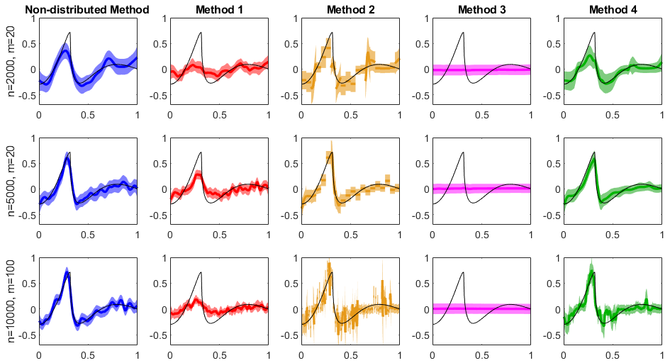
Figure 2: Adaptively scaled (MMLE) Matérn process prior ($\alpha=3$). Benchmark and distributed GP posteriors. True function $f_{0}(x)=\sum_{i=4}^{\infty}1.5i^{-3/2-\beta}\sin(i)\psi_{i}(x)$ drawn in black. Posterior means drawn by solid lines, surrounded by $95\%$ point-wise credible sets, shaded between two dotted lines. The five columns correspond (left to right) to the non-distributed method, the distributed method with random partitioning, and the distributed methods with spatial partitioning without smoothing, with inverse variance weights and with exponential weights. From top to bottom the sample sizes are $n=2000,5000,10000$ and the number of experts is $m=20,20,100$.

(n,m)	$(2000,20)$	$(5000,20)$	$(10000,100)$
BM	0.093 (0.016)	0.069 (0.009)	0.052 (0.007)
M1	0.189 (0.019)	0.120 (0.021)	0.176 (0.012)
M2	0.120 (0.020)	0.010 (0.009)	0.109 (0.001)
M3	0.225 (0.001)	0.224 (0.002)	0.226 ($<$0.001)
M4	0.100 (0.021)	0.066 (0.009)	0.087 (0.083)

((a)) Average $L_{2}$-distance between $f_{0}$ and posterior mean.

(n,m)	$(2000,20)$	$(5000,20)$	$(10000,100)$
BM	0.183 (0.025)	0.137 (0.022)	0.103 (0.007)
M1	0.122 (0.069)	0.129 (0.037)	0.113 (0.046)
M2	0.194 (0.031)	0.138 (0.018)	0.177 (0.011)
M3	0.100 (0.003)	0.093 (0.003)	0.100 (0.001))
M4	0.157 (0.019)	0.121 (0.009)	0.138 (0.004)

((b)) Average radius credible ball.

Table 4: Data-based rescaled (MMLE) Matérn Gaussian process prior. BM: Benchmark, Non-distributed method. M1: Random partitioning, M2: Spatial partitioning, M3: Spatial partitioning with inverse variance weights, M4: Spatial partitioning with exponential weights.

(n,m)	$(1000,5)$	$(5000,20)$	$(10000,100)$
BM	1.00	1.00	1.00
M1	0.18	0.57	0.15
M2	0.98	1.00	1.00
M3	0.00	0.00	0.00
M4	0.96	1.00	1.00

Table 5: Data-based rescaled (MMLE) Matérn Gaussian process prior. Proportion of experiments when the true function $f_{0}$ was inside in the $L_{2}$-credible ball.

(n,m)	$(1000,5)$	$(5000,20)$	$(10000,100)$
Benchmark	35.85s (6.48s)	662.4s (26.9s)	4726s (570s)
Random	4.97s (1.32s)	13.8s (3.9s)	23.7s (4.6s)
Spatial	5.25s (2.49s)	13.0s (3.4s)	24.8s (6.4s)

Table 6: Data-based rescaled (MMLE) Matérn Gaussian process prior. Average run time for computing the posterior. Benchmark: Non-distributed method. Method 1: Random partitioning, Method 2: Spatial partitioning.

4.2.2 Squared exponential kernel

The squared exponential process is the centered Gaussian process with covariance kernel $\operatorname{\mathbb{E}}(G_{s}G_{t})=e^{-|s-t|^{2}/2}$. Its sample paths are infinitely smooth, but with appropriately changed length scale the process is an accurate prior also for finitely smooth functions $f_{0}$ (see vandervaart2009 ). The optimal length scale for a $\beta$ regular function $f_{0}$ is $\tau_{n}=n^{1/(1+2\beta)}$. In our study we generated data with the function $f_{0}$ as described previously with $c=6$ and $\beta=3/2$.

We considered pairs of sample sizes and numbers of machines $(n,m)$ equal to $(1000,5)$, $(5000,10)$ and $(10000,100)$. For each setting and both with deterministic and adaptive, data-based length scale, we report the average performance over 100 independent data sets, except in the adaptive setting with $(n,m)=(10000,100)$, where we considered only 20 repetitions, due to the overly slow non-distributed approach.

For visualising our numerical findings, we plot the posterior means and the pointwise $95\%$-credible sets in Figures 3 and 4 for the deterministic and adaptive priors, respectively.

Tables (7(a))–9 report the average $L_{2}$-errors, credible radii, $L_{2}$-coverages of credible sets and run times in the scenarios with deterministic scaling. The errors were comparable for all methods and coverage was excellent, while the size of the credible sets were somewhat smaller for the true posterior (BM) and the random distributed technique (M1). The run times of the distributed algorithms were similar and substantially shorter than for the true (non-distributed) posterior.

Tables 10(a)-12 report the same quantities for the adaptive priors, with data-based length scale. In all investigated settings the consensus Monte-Carlo method (M1) performed substantially worse than the true posterior (BM), as was expected from the fact that this method of distribution cannot adapt to unknown smoothness. The standard spatially distributed approach (M2) provided good estimation and reliable uncertainty quantification. The aggregation method (M3) proposed in the literature performed also sub-optimally, whereas our approach with exponential weights (M4) outperformed the other distributed approaches. The run times of the distributed methods were substantially shorter than for the standard, non-distributed algorithm. We note again, that these run times are sequential and could be substantially shortened by parallelising the computations. For instance, in the last scenario $(10000,100)$ our approach (M4) would take a fraction of a second (around 0.2s) as compared to the average runtime of 4741s of the non-distributed algorithm, while providing comparable reliability and accuracy.

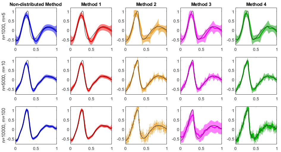
Figure 3: Deterministically (optimally) scaled squared exponential prior. Benchmark and distributed GP posteriors. True function $f_{0}(x)=\sum_{i=4}^{\infty}6^{-2}\sin(i)\psi_{i}(x)$ drawn in black. Posterior means drawn by solid lines, surrounded by $95\%$ point-wise credible sets, shaded between two dotted lines. The five columns correspond (left to right) to the non-distributed method, the distributed method with random partitioning, and the distributed methods with spatial partitioning without smoothing, with inverse variance weights and with exponential weights. From top to bottom the sample sizes are $n=2000,5000,10000$ and the numbers of experts are $m=20,20,100$.

(n,m)	$(1000,5)$	$(5000,10)$	$(10000,100)$
BM	0.153 (0.014)	0.080 (0.006)	0.060 (0.007)
M1	0.154 (0.014)	0.080 (0.006)	0.062 (0.006)
M2	0.143 (0.016)	0.070 (0.009)	0.101 (0.008)
M3	0.131 (0.017)	0.062 (0.008)	0.123 (0.008)
M4	0.131 (0.016)	0.063 (0.009)	0.079 (0.007)

((a)) Average $L_{2}$-distance between $f_{0}$ and posterior mean.

(n,m)	$(1000,5)$	$(5000,10)$	$(10000,100)$
BM	0.172 (0.001)	0.096 ($<$0.001)	0.075 ($<$0.001)
M1	0.175 (0.001)	0.097 ($<$0.001)	0.083 ($<$0.001)
M2	0.220 (0.001)	0.138 ($<$0.001)	0.208 ($<$0.001)
M3	0.235 (0.001)	0.148 ($<$0.001)	0.308 ($<$0.001))
M4	0.224 (0.012)	0.141 ($<$0.001)	0.209 ($<$0.001)

((b)) Average radius $r$ of the $L_{2}$-credible ball.

Table 7: Deterministically (optimally) rescaled squared exponential Gaussian process prior. BM: Benchmark, Non-distributed method, M 1: Random partitioning, M 2: Spatial partitioning, M 3: Spatial partitioning with inverse variance weights, M 4: Spatial partitioning with exponential weights. Average values over 100 replications with standard error in brackets.

(n,m)	$(1000,5)$	$(5000,10)$	$(10000,100)$
BM	0.95	0.99	1.00
M1	0.94	1.00	1.00
M2	1.00	1.00	1.00
M3	1.00	1.00	1.00
M4	1.00	1.00	1.00

Table 8: Deterministically (optimally) scaled squared exponential prior. Proportion of runs when the $L_{2}$-credible ball contains $f_{0}$.

(n,m)	$(1000,5)$	$(5000,10)$	$(10000,100)$
Benchmark	0.094s (0.018s)	9.035s (0.942s)	59.95s (17.22s)
Random	0.023s (0.004s)	0.482s (0.092s)	0.50s (0.22s)
Spatial	0.048s (0.012s)	0.568 (0.084s)	1.14s 0.52s)

Table 9: Deterministically (optimally) scaled squared exponential prior. Average run time (and standard error) for computing the posterior. Benchmark: Non-distributed method, Method 1: Random partitioning, Method 2: Spatial partitioning.

(n,m)	$(1000,5)$	$(5000,10)$	$(10000,100)$
BM	0.212 (0.127)	0.065 (0.008)	0.050 (0.007)
M1	0.350 (0.053)	0.305 (0.050)	0.348 (0.009)
M2	0.128 (0.021)	0.073 (0.009)	0.117 (0.008)
M3	0.349 (0.050)	0.364 (0.020)	0.396 (0.001)
M4	0.138 (0.030)	0.069 (0.011)	0.095 (0.007)

((a)) Average $L_{2}$-distance between $f_{0}$ and posterior mean.

(n,m)	$(1000,5)$	$(5000,10)$	$(10000,100)$
BM	0.165 (0.069)	0.113 (0.008)	0.088 (0.005)
M1	0.098 (0.049)	0.065 (0.033)	0.047 (0.014)
M2	0.208 (0.024)	0.119 (0.008)	0.188 (0.096)
M3	0.127 (0.050)	0.086 (0.008)	0.106 (0.002))
M4	0.197 (0.022)	0.114 (0.007)	0.170 (0.004)

((b)) Average size of the credible balls.

Table 10: Data-based rescaled (MMLE) squared exponential Gaussian process prior. BM: Benchmark, Non-distributed method. M1: Random partitioning, M2: Spatial partitioning, M3: Spatial partitioning with inverse variance weights, M4: Spatial partitioning with exponential weights. We report the average (and standard deviations) out of 100 repetitions (except of the last column when the number are based on 20 repetitions)

(n,m)	$(1000,5)$	$(5000,10)$	$(10000,100)$
BM	0.66	1.00	1.00
M1	0.01	0.01	0.00
M2	1.00	1.00	1.00
M3	0.06	0.00	0.00
M4	0.91	0.99	1.00

Table 11: Data-based rescaled (MMLE) squared exponential Gaussian process prior. Proportion of runs when the $L_{2}$-credible ball contains $f_{0}$.

(n,m)	$(1000,5)$	$(5000,10)$	$(10000,100)$
Benchmark	14.84s (5.23s)	633.8s (241.2s)	4741s (1069s)
Random	2.37s (1.14s)	24.7s (5.1s)	22.0s (6.1s)
Spatial	2.55s (1.11s)	25.2s (5.4s)	22.6s (5.8s)

Table 12: Data-based rescaled (MMLE) squared exponential Gaussian process prior. Average run time for the computation of the posterior. Benchmark: Non-distributed method. Method 1: Random partitioning, Method 2: Spatial partitioning.

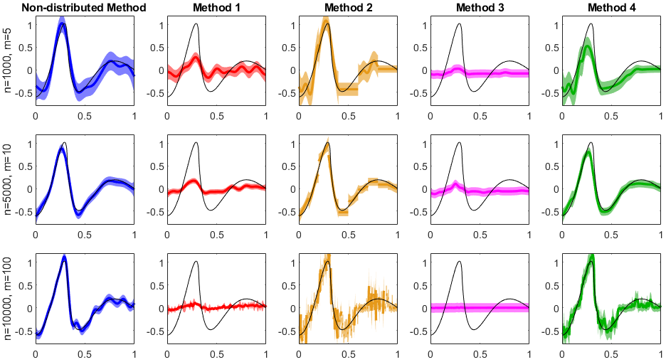
Figure 4: Data-based rescaled (MMLE) squared exponential Gaussian process prior. Benchmark and distributed GP posteriors. True function $f_{0}(x)=\sum_{i=4}^{\infty}6^{-2}\sin(i)\psi_{i}(x)$ drawn in black. Posterior means drawn by solid lines, surrounded by $95\%$ point-wise credible sets, shaded between two dotted lines. The five columns correspond (left to right) to the non-distributed method, the distributed method with random partitioning, and the distributed methods with spatial partitioning without smoothing, with inverse variance weights and with exponential weights. From top to bottom the sample sizes are $n=2000,5000,10000$ and the numbers of experts are $m=20,20,100$.

4.3 Real world dataset: Airline Delays (USA Flight)

Next we compare the performance of the different distributed methods on a large-scale real world data set consisting of the flight arrival and departure times of all commercial flights in the USA from January 2008 to April 2008. This data set covers almost 6 million flights and contains exhaustive information about them, including delays at arrival (in minutes). For a such large data set standard non-parametric Bayesian regression is impossible, and approximate algorithms must be used.

This data set has been studied before in hensman:fusi:lawrence:2013 ; gal:vdwilk:rasmussen:2014 ; ng:deisenroth:14 ; deisenroth2015 using various approximation techniques to speed-up the GP regression with squared exponential covariance kernel. In hensman:fusi:lawrence:2013 Stochastic Variational inference (SVI) was applied based on the inducing points variational method proposed by Titsias titsias:2009 . In deisenroth2015 various distributed methods with random partitioning were compared, amongst which robust Bayesian Committee Machine (rBCM) performed the best. In our numerical analysis we use these two approaches as benchmark to compare our methods.

We follow the procedure described by hensman:fusi:lawrence:2013 , and applied also in deisenroth2015 , to predict the flight delay in minutes at arrival. We select $P=70K,2M$ or $5M$ data points to train our models and use an additional $100,000$ data points for testing. We select the same eight-dimensional input variable $x$ consisting of: the age of the aircraft (number of years since deployment), distance between the two airports (in miles), airtime (in minutes), departure time, arrival time, month, day of the week and day of the month. To account to the increasing sample sizes, we chose the number of experts in methods M1-M4 as 256, 512 and 1024 in the three scenarios, respectively. The root-mean-square errors (RMSE, i.e. root of the mean of the squares of the deviations within the training set) of the different methods are reported in Table 13, along with the reported performance of the SVI and the rBCM. All simulations were carried out on a single workstation, computing the different local GP posteriors sequentially, storing the results on the single work station.

Method $\backslash P=$	$70K$	$2M$	$5M$
SVI	33.0	$-$	$-$
rBCM	27.1	34.4	35.5
M1	29.1	34.8	41.5
M2	25.0	27.1	30.2
M3	33.4	40.4	45.1
M4	26.6	31.5	31.8

Table 13: US Flight Data Set. Root-mean-square error (RMSE) of different scalable GP methods. SVI and rBCM results are reported from hensman:fusi:lawrence:2013 and deisenroth2015 , respectively. M1: Random partitioning, M2: Spatial partitioning, M3: Spatial partitioning with inverse variance weights, M4: Spatial partitioning with exponential weights.

In Table 13 one can observe a decrease in performance with the number of training data, which was reported before in deisenroth2015 . It is also noticeable that randomly partitioning the data over the machines leads to similar RMSE as obtained by rBCM, which is not surprising in view of the above simulation study. In contrast, spatial partitioning (M2) consistently outperforms all the other GP methods. However, the inherently induced discontinuities of this procedure make it visually unappealing. Using continuous weights solves the problem of discontinuities, but can result in highly sub-optimal performance when using inverse variance weights (M3). Our proposal to use exponential weights (M4) remedies this problem and largely improves the prediction. The run time of methods M1-M4 ranged between 20 and 45 minutes in all experiments. We note that they were not optimised by parallelisation, which would further reduce the computational times substantially, even by a factor of 1000 in the last scenario with $P=5M$.

5 Discussion

The paper provides the first theoretical guarantees for method of spatial distribution applied to Gaussian processes. Our general results show that the resulting approximation to the posterior provides optimal recovery (both in the case of known and unknown regularity parameter) of the underlying functional parameter of interest in a range of models, including the nonparametric regression model with Gaussian errors and the logistic regression model. As specific examples of priors we considered the popular Matérn process and integrated Brownian motion, but in principle other GP priors could be covered as well. The theoretical findings are complemented with a numerical analysis both on synthetic and real world data sets, where we also proposed a novel aggregation technique for aggregating the local posteriors together, which empirically outperformed the close competitors.

The main advantage of spatial distribution of the data is the ability to adapt the length scale of the prior in a data-driven way, which was highlighted by both theory and numerical illustration. The latter showed that the combination technique of the local posteriors is highly important and can substantially influence the performance of the method.

Our results, although formulated for Gaussian processes, in principle rely on general Bayesian nonparametric techniques, adapted to the spatially distributed architecture and hence can be potentially extended to other classes of priors. Also, in the theoretical results univariate functional parameters were considered for simplicity, but the results could be extended to higher dimensional covariates. Another interesting extension is to derive theoretical guarantees for the proposed aggregation techniques beyond the “glue together” approach covered by this paper. These extensions, although of interest, are left for future work.

6 Proofs of the general results

In this section we collect the proofs of the general contraction rate theorems for the non-adaptive and adaptive frameworks with known and unknown regularity parameter, respectively.

6.1 Proof of Theorem 2

The $k$th local problem is a non-i.i.d. regression problem of the type considered in ghoshal:vaart:2007 , with a Gaussian process prior as considered in vaart:zanten:2008 , but with the number of observations reduced to $n/m$. These papers give a rate of contraction of the local posterior distribution $\Pi^{(k)}(\cdot|\textbf{Y}^{(k)})$ relative to the root of the average square Hellinger distance defined as

$$d_{n}^{(k)}(f,g)^{2}=\frac{m}{n}\sum_{x_{i}\in\mathcal{D}^{(k)}}\int(\sqrt{p_{f,i}}-\sqrt{p_{g,i}})^{2}d\mu_{i}.$$

Under Assumption 1 this square semimetric is bounded above by the square of the local uniform metric $\|\cdot\|_{\infty,k}$ and so are the average local Kullback-Leibler divergence and variation. Therefore Theorem 4 of ghoshal:vaart:2007 shows that the solution $\varepsilon_{n}$ to the inequality $\phi_{f_{0}}^{(k)}(\varepsilon_{n})\leq(n/m)\varepsilon_{n}^{2}$ gives a rate of contraction relative to $d_{n}^{(k)}$. (Theorem 3.3 in vaart:zanten:2008 shows that in the Gaussian regression problem the same is true with the local root average square Hellinger distance replaced by the local empirical $L_{2}$-distance.) Inspection of the proof (or see (b) of Theorems 8.19-8.20 in ghosal2017fundamentals ) shows that this rate statement can be understood in the sense that

$$\operatorname{\mathbb{E}}_{0}\Pi^{(k)}\left(f:\,d_{n}^{(k)}(f,f_{0})^{2}\geq M_{n}\varepsilon_{n}^{2}|\textbf{Y}^{(k)}\right)\lesssim\frac{1}{(n/m)\varepsilon_{n}^{2}},$$ (20)

thus including the assertion that the left side tends to zero at the speed $m/(n/\varepsilon_{n}^{2})$. Then, because $d_{n}^{2}=m^{-1}\sum_{k=1}^{m}(d_{n}^{(k)})^{2}$,

$$\operatorname{\mathbb{E}}_{0}\Pi_{n,m}\left(f:\,d_{n}(f,f_{0})^{2}\geq M_{n}\varepsilon_{n}^{2}|\textbf{Y}\right)$$

$$\quad\leq\operatorname{\mathbb{E}}_{0}\Pi_{n,m}\left(f:\,\exists k\ d_{n}^{(k)}(f,f_{0})^{2}\geq M_{n}\varepsilon_{n}^{2}|\textbf{Y}\right)$$

$$\quad\leq\sum_{k=1}^{m}\operatorname{\mathbb{E}}_{0}\Pi^{(k)}\left(f:\,d_{n}^{(k)}(f,f_{0})^{2}\geq M_{n}\varepsilon_{n}^{2}|\textbf{Y}^{(k)}\right)\lesssim\frac{m^{2}}{n\varepsilon_{n}^{2}},$$

which tends to zero by the assumption that $n\varepsilon_{n}^{2}/m^{2}\rightarrow\infty$. This concludes the proof of the first statement of the theorem.

Theorems 8.19-8.20 in ghosal2017fundamentals show that the left side of (20) is bounded by the probability of failure of the evidence lower bound (the left side of Lemma 8.21) plus terms of the order $e^{-D(n/m)\varepsilon_{n}^{2}}$, for some positive constant $D$. Under Assumption 1 the former probability gives the order on the right side of (20). We show below in Lemma 15 that in the nonparametric and logistic regression models the probability of failure of the evidence lower bound is actually also of the smaller exponential order, whence the right side of (20) can be replaced by $e^{-D(n/m)\varepsilon_{n}^{2}}$. The right side of the final display in the preceding proof then improves to $me^{-D(n/m)\varepsilon_{n}^{2}}$, which tends to zero if $m\leq n\varepsilon_{n}^{2}/(D^{\prime}\log n)$ for a sufficiently large constant $D^{\prime}$. This proves the second statement of the theorem.

6.2 Proof of Theorem 3

Under Assumption 1 the average square local Hellinger distance $d_{n}^{(k)}$ and the local average Kullback-Leibler divergence and variation are bounded above by the square local uniform norm. Therefore conditions (9)-(11) imply the conditions of Theorem 4 of ghoshal:vaart:2007 applied to the $k$th local problem, with $n/m$ observations and prior $\Pi^{A,(k)}$. Thus this theorem gives a contraction rate $\varepsilon_{n}$ of the $k$th local posterior distribution relative to $d_{n}^{(k)}$. In view of (b) of Theorems 8.19-8.20 in ghosal2017fundamentals , this rate can be understood in the sense of (20), with $\Pi^{A,(k)}$ taking the place of $\Pi^{(k)}$, and improved to exponential order in the case of the Gaussian and logistic regression models. The proof can be finished as the proof of Theorem 2.

7 Proofs for the examples

In this section we collect the proofs of the corollaries for the integrated Brownian motion and Matérn prior processes.

7.1 Proof of Corollary 4

Assumption 1 holds both in the nonparametric and logistic regression models, and for $\varepsilon_{n}=n^{-\beta/(2\beta+1)}$ we have $n\varepsilon_{n}^{2}=n^{1/(2\beta+1)}$ so that $m=o(n\varepsilon_{n}^{2}/\log n)$ by assumption. Therefore the corollary is a consequence of Theorem 2 provided the remaining condition of this theorem, the modulus inequalities $\phi_{f_{0}}^{(k)}(\varepsilon_{n})\leq(n/m)\varepsilon_{n}^{2}$, is satisfied.

Let $(G^{\tau,(k)}_{t}:t\in I^{(k)})$ be rescaled Integrated Brownian motion (14) on the interval $I^{(k)}$ and let $\mathbb{H}^{\tau,(k)}$ be its RKHS. We prove below that, for $f_{0}\in C^{\beta}([0,1])$ and $\beta\leq\ell+1/2$, if $m\leq\tau/\varepsilon^{1/(\ell+1/2)}$ and $B_{n}\geq\varepsilon$ with

$$\frac{B_{n}^{2}}{m}\gtrsim\varepsilon^{2(1+(\ell-\beta)\wedge 0)/\beta}(\tau\vee\tau^{2\ell+1}),$$ (21)

then the following bounds are satisfied up to constants that do not depend on $\varepsilon$, $\tau$, $m$ and $n$

$$\inf_{h:\|f_{0}-h\|_{\infty,k}\leq\varepsilon}\|h\|^{2}_{\mathbb{H}^{\tau,(k)}} \lesssim\frac{\tau^{-2\ell-1}}{m\varepsilon^{\frac{2\ell+2-2\beta}{\beta}}},$$ (22)

$$-\log\Pr\bigl{(}\|G^{\tau,(k)}\|_{\infty,k}\!<\!\varepsilon\bigr{)} \lesssim\frac{\tau}{m\varepsilon^{\frac{1}{\ell+1/2}}}+\log\!\frac{B_{n}(\tau^{\ell}\!\vee\!1)}{\varepsilon^{2}}.$$ (23)

(More precisely, (22) needs (21), but (23) is valid without it.) Next we choose $\tau=\tau_{n}\asymp n^{\frac{\ell+1/2-\beta}{(\ell+1/2)(2\beta+1)}}$ and $\varepsilon=\varepsilon_{n}=n^{-\beta/(2\beta+1)}$, so that condition (21) is satisfied if $B_{n}^{2}\geq mn^{\frac{-1+2(\ell-\beta)\vee 0}{1+2\beta}}$, which is true by assumption. Furthermore, with these choices $\tau_{n}/\varepsilon_{n}^{1/(\ell+1/2)}=n^{1/(1+2\beta)}\geq m$, by assumption, and $(\tau_{n}^{\ell}\vee 1)/\varepsilon_{n}$ is a power of $n$, so that the second term on the right side of (23) is bounded by a multiple of the first if $(\log B_{n}\vee 0)+\log n\leq n^{1/(1+2\beta)}/m$, which is also true by assumption. Combining (22) and (23), we then get

$$\phi_{f_{0}}^{(k)}(\varepsilon_{n})\lesssim\frac{\tau_{n}^{-2\ell-1}}{m\varepsilon_{n}^{(2\ell+2-2\beta)/\beta}}+\frac{\tau_{n}}{m\varepsilon_{n}^{1/(\ell+1/2)}}\lesssim\frac{n\varepsilon_{n}^{2}}{m}.$$

Proof of (22)

By Whitney’s theorem, a function $f_{0}\in C^{\beta}([0,1])$ can be extended to a function $f_{0}$ on the full line $\mathbb{R}$ of the same Hölder norm and with compact support. Let $\psi$ be a smooth $\ell$th order kernel (a function with $\int\psi(s)\,ds=1$, $\int s^{l}\psi(s)\,ds=0$ for all $l\leq\ell$, and $\int|s|^{\ell+1}|\psi(s)|\,ds<\infty$), and let $f_{0}\ast\psi_{\sigma}$ be the convolution between $f_{0}$ and the scaled version $\psi_{\sigma}(\cdot):=\sigma^{-1}\psi(\cdot/\sigma)$ of $\psi$, for $\sigma>0$. Then, for $l\in\mathbb{N}$,

$$\sup_{0\leq t\leq 1}|f_{0}-f_{0}\ast\psi_{\sigma}|(t) \lesssim\sigma^{\beta},$$ (24)

$$\sup_{0\leq t\leq 1}|(f_{0}\ast\psi_{\sigma})^{(l)}(t)| \lesssim\Bigl{(}\frac{1}{\sigma}\Bigr{)}^{(l-\beta)\vee 0}.$$ (25)

For proofs, see the proof of Lemma 11.31 in ghosal2017fundamentals , and at the end of this section.

The local RKHS $\mathbb{H}^{\tau,(k)}$ of $G^{\tau,(k)}$ is characterised in Lemma 8 and 9 below. Set $I^{(k)}=\left[\frac{k-1}{m},\frac{k}{m}\right]$ and consider the function $h$ defined by

$$h(t) :=I^{\ell+1}\left((f_{0}\ast\psi_{\sigma})^{(\ell+1)}\textbf{1}_{I^{(k)}}\right)(t)$$

$$\qquad+\sum_{r=0}^{\ell}\frac{(t-\frac{k-1}{m})^{r}}{r!}(f_{0}\ast\psi_{\sigma})^{(r)}\left(\frac{k-1}{m}\right).$$ (26)

The function $I^{\ell+1}\bigl{(}(f_{0}\ast\psi_{\sigma})^{(\ell+1)}\textbf{1}_{I^{(k)}}\bigr{)}$ has $(\ell+1)th$ derivative equal to $(f_{0}\ast\psi_{\sigma})^{(\ell+1)}\textbf{1}_{I^{(k)}}$ and derivatives of orders $0,1,\ldots,\ell$ at $(k-1)/m$ equal to 0, while the polynomial part of $h$ is set up to have vanishing $(\ell+1)$th derivative and derivatives of orders $0,1,\ldots,\ell$ at $(k-1)/m$ equal to the derivatives of $f_{0}\ast\psi_{\sigma}$ at this point. If follows that $h=f_{0}\ast\psi_{\sigma}$ on $I^{(k)}$, whence $\|h-f_{0}\|_{\infty,k}\leq\sigma^{\beta}$ by (24). Moreover, in view of Lemmas 8 and 9, the local RKHS norm of $h$ satisfies

$$\|h\|^{2}_{\mathbb{H}^{\tau,(k)}}\leq\sum_{j=0}^{\ell}\frac{h^{(j)}(0)^{2}}{B_{n}^{2}\tau^{2j}}+\frac{1}{\tau^{2\ell+1}}\int_{\frac{k-1}{m}}^{\frac{k}{m}}(f_{0}\ast\psi_{\sigma})^{(\ell+1)}(t)^{2}\,dt.$$

In view of (25) the second term in the right side is bounded from above by $\tau^{-2\ell-1}\sigma^{-2(\ell+1-\beta)}/m$. Because the first, integral part of $h$ vanishes at 0, only the polynomial part contributes to the first term of the RKHS norm. Without the factor $1/B_{n}^{2}$ this is equal to

$$\sum_{j=0}^{\ell}\frac{1}{\tau^{2j}}\biggl{(}\sum_{r=j}^{\ell}\Bigl{(}-\frac{k-1}{m}\Bigr{)}^{r-j}\frac{1}{(r-j)!}(f_{0}\ast\psi_{\sigma})^{(r)}\Big{(}\frac{k-1}{m}\Big{)}\biggr{)}^{2}$$

$$\quad\leq\sum_{j=0}^{\ell}\frac{1}{\tau^{2j}}\Bigl{(}\sum_{r=j}^{\ell}\frac{1}{\sigma^{(r-\beta)\vee 0}}\Bigr{)}^{2}\lesssim\Bigl{(}\frac{1}{\sigma}\Bigr{)}^{(2\ell-2\beta)\vee 0}(\tau^{-2\ell}\vee 1).$$

Taking these together and choosing $\sigma=\varepsilon^{1/\beta}$, we see that

$$\inf_{h:\|f_{0}-h\|_{\infty,k}\leq\varepsilon}\|h\|^{2}_{\mathbb{H}^{\tau,(k)}} \lesssim\frac{\tau^{-2\ell}\vee 1}{B_{n}^{2}\varepsilon^{\frac{2\ell-2\beta}{\beta}\vee 0}}+\frac{\tau^{-2\ell-1}}{m\varepsilon^{\frac{2\ell+2-2\beta}{\beta}}}.$$

Under assumption (21), the right side of this display is dominated by its second term. This concludes the proof of assertion (22).

Proof of (23)

By the independence of the two components of the process $G^{\tau,(k)}$, defined in (14),

$$\Pr\bigl{(}\|G^{\tau,(k)}\|_{\infty,k}<\varepsilon\bigr{)}$$

$$\ \geq\Pr\Bigl{(}\|I^{\ell}W_{\tau t}\|_{\infty,k}<\frac{\varepsilon}{2}\Bigr{)}\Pr\Big{(}\Bigl{\|}B_{n}\sum_{j=0}^{\ell}\frac{Z_{j}(\tau t)^{j}}{j!}\Bigr{\|}_{\infty,k}<\frac{\varepsilon}{2}\Big{)}.$$

In view of Lemma 10 (with $x_{0}=\tau(k-1)/m$ and $x_{1}=\tau k/m$), the first term on the right, the small ball probability of the scaled $\ell$-fold integrated Brownian motion on $I^{(k)}$, is bounded from below by a multiple of

$$\exp\Big{\{}-q\frac{\tau/m}{\varepsilon^{1/(\ell+1/2)}}-\log\frac{2}{\varepsilon}\Big{\}},$$

for some $q>0$, provided that $(\tau/m)\varepsilon^{-1/(\ell+1/2)}\geq 1$. On the other hand, by the independence of the random variables $Z_{j}$, the second term is bounded below by

$$\Pr\Bigl{(}\max_{0\leq j\leq\ell}|Z_{j}|<\frac{\varepsilon}{2B_{n}e(\tau^{\ell}\lor 1)}\Bigr{)}$$

$$\qquad=\Big{(}2\Phi\Bigl{(}\frac{\varepsilon}{2B_{n}e(\tau^{\ell}\lor 1)}\Bigr{)}-1\Big{)}^{\ell+1}\gtrsim\Big{(}\frac{\varepsilon}{B_{n}e(\tau^{\ell}\lor 1)}\Big{)}^{\ell+1},$$

provided $4B_{n}e>\varepsilon$, since $2\Phi(x)-1\geq xe^{-1}$, for $0<x<2$. Combining the last two displays, we find (23).

Proof of (25)

The derivative of the convolution $f\ast g$ is given as $\left(f\ast g\right)^{\prime}=f^{\prime}\ast g=f\ast g^{\prime}$, which can be iterated to obtain derivatives of higher degree. In the case that $\beta>l$ we use this to see that $(f_{0}\ast\psi_{\sigma})^{(l)}=f_{0}^{(l)}\ast\psi_{\sigma}$, which is uniformly bounded by $\|f_{0}^{(l)}\|_{\infty}$. In the case that $\beta\leq l$, we write $(f_{0}\ast\psi_{\sigma})^{(l)}=f_{0}^{(b)}\ast\psi^{(l-b)}_{\sigma}$, for $b$ the largest integer strictly smaller than equal $\beta$. Since $\psi$ is smooth and integrates to 1, we have $\int\psi^{(l)}(s)\,ds=0$, for $l=1,2,\ldots$. Therefore

$$(f_{0}\ast\psi_{\sigma})^{(l)}(t)=\int\bigl{(}f_{0}^{(b)}(t-\sigma y)-f_{0}^{(b)}(t)\bigr{)}\psi^{(l-b)}(s)\,ds\frac{1}{\sigma^{l-b}}.$$

Since $f_{0}^{(b)}\in C^{\beta-b}$, this is bounded in absolute value by $\int|\sigma y|^{\beta-b}|\psi^{(l-b)}(s)|\,ds\,\sigma^{-l+b}\lesssim\sigma^{\beta-l}$.

7.2 Proof of Corollary 5

In view of Theorem 3 it is sufficient to construct a sieve $B_{n,m}^{(k)}$ such that assumptions (9), (10) and (11) hold. This may be done analogously to the construction in vandervaart2009 for the squared exponential Gaussian process.

For $\mathbb{H}_{1}^{\tau,(k)}$ the unit ball in the RKHS of the local rescaled integrated Brownian motion $(G^{\tau,(k)}_{t}:t\in I^{(k)})$ with fixed scale $\tau$, and $\mathbb{B}^{(k)}_{1}$ the unit ball in the Banach space of continuous functions on $I^{(k)}$ equipped with the supremum norm $\|\cdot\|_{\infty,k}$, we consider sieves of the form

$$B_{n,m}^{(k)}=\bigl{\{}f1_{I^{(k)}}:f\in\bigcup_{q_{n}<\tau<r_{n}}K_{n,m}\mathbb{H}_{1}^{\tau,(k)}+\varepsilon_{n}\mathbb{B}^{(k)}_{1}\bigr{\}}.$$ (27)

In the present proof we set $\varepsilon_{n}=Cn^{-\beta/(2\beta+1)}$, $q_{n}=0$, $r_{n}=cn^{\frac{\ell+1/2-\beta}{(\ell+1/2)(2\beta+1)}}$, and $K^{2}_{n,m}:=K(n/m)\varepsilon_{n}^{2}$, for large constants $C$, $c$ and $K$ to be determined.

Write $G^{A,(k)}$ for the rescaled integrated Brownian motion process with random scale $\tau$. It will be shown below that the following bounds are satisfied

$$\log\Pr\left(G^{A,(k)}\notin B^{(k)}_{n,m}\right) \leq-4\frac{n}{m}\varepsilon_{n}^{2},$$ (28)

$$-\log\Pr\left(\|G^{A,(k)}-f_{0}\|_{\infty,k}\leq\varepsilon_{n}\right) \leq\frac{n}{m}\varepsilon_{n}^{2},$$ (29)

$$\log N\left(\varepsilon_{n},B^{(k)}_{n,m},\|\cdot\|_{\infty,k}\right) \lesssim\frac{n}{m}\varepsilon_{n}^{2}.$$ (30)

This verifies (9)–(11) and completes the proof of the corollary.

Proof of (28)

The local remaining masses satisfy

$$\Pr (G^{A,(k)}\notin B_{n,m}^{(k)})$$

$$\leq\Pr(\tau>r_{n})+\int_{0}^{r_{n}}\Pr(G^{\tau,(k)}\notin B_{n,m}^{(k)})g(\tau)\,d\tau.$$

By assumption (15), the first term is bounded above by a multiple of $\exp\bigl{(}-D_{1}n^{1/(2\ell+2)}r_{n}^{(\ell+1/2)/(\ell+1)}/(2m)\bigr{)}\leq\exp(-5(n/m)\varepsilon_{n}^{2})$, if the constant $c$ in $r_{n}$ is chosen small enough relative to $C$ in $\varepsilon_{n}$ and $D_{1}$. It suffices to bound the second term.

Let $\phi_{0}^{\tau,(k)}(\varepsilon)=-\log\Pr\bigl{(}\|G^{\tau,(k)}\|_{\infty,k}<\varepsilon\bigr{)}$ be the centered small ball exponent of the rescaled process $G^{\tau,(k)}$. Then

$$\Pr(G^{\tau,(k)}\notin B_{n,m}^{(k)}) \leq\Pr(G^{\tau,(k)}\notin K_{n,m}\mathbb{H}_{1}^{\tau,(k)}+\varepsilon_{n}\mathbb{B}^{(k)}_{1})$$

$$\leq 1-\Phi(\Phi^{-1}(e^{-\phi_{0}^{\tau,(k)}(\varepsilon_{n})})+K_{n,m}),$$ (31)

in view of Borell’s inequality (see borell1975brunn or Theorem 5 in vaart:zanten:2008:reproducing ). For $\tau\leq r_{n}$ and $\tau/m\geq\varepsilon_{n}^{1/(\ell+1/2)}$, relation (23) gives that $\phi_{0}^{\tau,(k)}(\varepsilon_{n})\lesssim r_{n}\varepsilon_{n}^{-1/(\ell+1/2)}/m+(0\vee\log B_{n})+\log n$, which is bounded above by $Kn\varepsilon_{n}^{2}/(8m)=K_{n,m}^{2}/8$, for sufficiently large $K$. For $\tau\leq r_{n}$ and $\tau/m\leq\varepsilon_{n}^{1/(\ell+1/2)}$, relation (23) applied with $\varepsilon=(\tau/m)^{\ell+1/2}\leq\varepsilon_{n}$, so that $\tau/m\geq\varepsilon^{1/(\ell+1/2)}$, gives that $\phi_{0}^{\tau,(k)}(\varepsilon_{n})\leq\phi_{0}^{\tau,(k)}(\varepsilon)\lesssim 1+(0\vee\log B_{n})+\log n\ll K_{n,m}^{2}/8$. Therefore, Lemma 16 gives that $\Phi^{-1}(e^{-\phi_{0}^{\tau,(k)}(\varepsilon_{n})})\geq-K_{n,m}/2$, and consequently the preceding display is bounded above by $1-\Phi(K_{n,m}/2)\leq e^{-K_{n,m}^{2}/8}$, by Lemma 17. This implies (28), for $K\geq 32$.

Proof of (29)

For $\tau\in[r_{n},2r_{n}]$, we have that $\tau/\varepsilon_{n}^{1/(\ell+1/2)}\asymp n\varepsilon_{n}^{2}$ and hence $\tau/m\geq\varepsilon_{n}^{1/(\ell+1/2)}$, by the assumptions on $m$, and condition (21) is satisfied at $\varepsilon=\varepsilon_{n}/2$, by the assumptions on $B_{n}$. Therefore, assertions (22) and (23) give

$$\phi^{\tau,(k)}_{f_{0}}(\varepsilon_{n}/2) \lesssim\frac{\tau^{-2\ell-1}}{m\varepsilon_{n}^{\frac{2\ell+2-2\beta}{\beta}}}+\frac{\tau}{m\varepsilon_{n}^{\frac{1}{\ell+1/2}}}+\log\frac{B_{n}(\tau^{\ell}\vee 1)}{\varepsilon_{n}^{2}}.$$

The first two terms on the right are both of the order $n\varepsilon_{n}^{2}/m$, where the multiplicative constant can be adjusted to be arbitrarily small by choosing the constant $C$ in $\varepsilon_{n}$ large, for a given constant $c$ in $r_{n}$. The third term is bounded above by a multiple of $(0\vee\log B_{n})+\log n\leq n^{1/(2\beta+1)}/m+\log n$, by assumption, and hence is also bounded by an arbitrarily small constant times $n\varepsilon_{n}^{2}/m$ if the constant $C$ in $\varepsilon_{n}$ is sufficiently large. Thus $C$ can be adjusted so that right side and hence $\phi^{\tau,(k)}_{f_{0}}(\varepsilon_{n}/2)$ is bounded above by $n\varepsilon_{n}^{2}/(2m)$. Then, in view of Lemma 5.3 in vaart:zanten:2008:reproducing ,

$$\Pr\big{(} \|G^{A,(k)}-f_{0}\|_{\infty,k}\leq\varepsilon_{n}\big{)}\geq\int_{0}^{\infty}e^{-\phi^{\tau,(k)}_{f_{0}}(\varepsilon_{n}/2)}g(\tau)\,d\tau$$

$$\geq\int_{r_{n}}^{2r_{n}}e^{-n\varepsilon_{n}^{2}/(2m)}g(\tau)\,d\tau.$$

In view of (15), minus the logarithm of this is bounded above by

$$-\log r_{n}+\frac{n\varepsilon_{n}^{2}}{2m}+D_{2}\frac{n^{1/(2\ell+2)}(2r_{n})^{(\ell+1/2)/(\ell+1)}}{m}.$$

The first term is of order $\log n$ and is much smaller than the second by the assumptions on $m$. The third term is of order $n\varepsilon_{n}^{2}/m$, where the multiplicative constant can be adjusted to be arbitrarily small by choosing $C$ in $\varepsilon_{n}$ sufficiently large. Thus the whole expression is bounded above by $n\varepsilon_{n}^{2}/m$.

Proof of (30)

By the combination of Lemmas 8 and 9, the RKHS $\mathbb{H}^{\tau,(k)}$ is the set of functions $h:I^{(k)}\to\mathbb{R}$ that can be extended to a function in the Sobolev space $H^{\ell+1}([0,1])$, equipped with the norm with square

$$\|h\|_{\mathbb{H}^{\tau,(k)}}^{2}=\inf_{\begin{subarray}{c}g\in H^{\ell+1}([0,1])\\ g1_{I^{(k)}}=h\end{subarray}}\sum_{j=0}^{\ell}\frac{g^{(j)}(0)^{2}}{B^{2}\tau^{2j}}+\frac{1}{\tau^{2\ell+1}}\int_{0}^{1}g^{(\ell+1)}(s)^{2}\,ds.$$

Because the norm $\tau\mapsto\|h\|_{\mathbb{H}^{\tau,(k)}}$ is decreasing in $\tau$, the unit balls satisfy $\mathbb{H}^{\tau,(k)}_{1}\subset\mathbb{H}^{r_{n},(k)}_{1}$ for $\tau\leq r_{n}$. It follows that

$$N\Bigl{(}2\varepsilon_{n},B_{n,m}^{(k)},\|\cdot\|_{\infty,k}\Bigr{)}\leq N\left(\varepsilon_{n}/K_{n,m},\mathbb{H}^{r_{n},(k)}_{1},\|\cdot\|_{\infty,k}\right).$$

Next we bound the covering number on the right using the estimate (23) on the small ball probability and the duality between these quantities, proved by KuelbsLi (see Lemma I.29(ii) in ghosal2017fundamentals ). By (23) the small ball exponent satisfies $\phi_{0}^{r_{n},(k)}(\varepsilon_{n})\lesssim(r_{n}/m)\varepsilon_{n}^{-1/(\ell+1/2)}$. Because $\Pr\bigl{(}\|G^{\tau,(k)}\|_{k,\infty}<\varepsilon\bigr{)}\leq\Pr\|I^{l}W\|_{k,\infty}<\varepsilon\bigr{)}$, by Anderson’s lemma, Lemma 10 gives that also $\phi_{0}^{r_{n},(k)}(\varepsilon_{n})\gtrsim(r_{n}/m)\varepsilon_{n}^{-1/(\ell+1/2)}$. Thus Lemma I.29(ii) gives

$$\log N\Bigl{(}\frac{\varepsilon_{n}}{\sqrt{D_{2}\frac{r_{n}}{m}\varepsilon_{n}^{-1/(\ell+1/2)}}},\mathbb{H}^{r_{n},(k)}_{1},\|\cdot\|_{\infty,k}\Bigr{)}\lesssim\!\frac{r_{n}}{m}\varepsilon_{n}^{-1/(\ell+1/2)}.$$

Because $K_{n,m}^{2}\asymp(r_{n}/m)\varepsilon_{n}^{-1/(\ell+1/2)}=n\varepsilon_{n}^{2}/m$, this gives the desired bound on the right side of the second last display and hence concludes the proof of (30).

7.3 Proof of Corollary 6

Let $G^{\tau,(k)}$ be the Matérn process with regularity parameter $\alpha$ scaled by $\tau$, write $\mathbb{H}^{\tau,(k)}$ for its RKHS and let $\phi_{f_{0}}^{\tau,(k)}(\varepsilon)=-\log\Pr(\|G^{\tau,(k)}-f_{0}\|_{\infty,k}<\varepsilon)$ be its small ball probability when restricted to $I^{(k)}$. We show below that for $f_{0}\in C^{\beta}([0,1])$ with $1/2<\beta\leq\alpha$, and $(\tau/m)\varepsilon^{-1/\alpha}\gtrsim\log(m/(\tau\varepsilon^{2}))$ and $\tau\lesssim\varepsilon^{-1/\beta}$, the following bounds are satisfied with multiplicative constants not depending on $\alpha$, $\varepsilon$, $m$, $\tau$ and $n$:

$$\inf_{h:\|f_{0}-h\|_{\infty,k}\leq\varepsilon}\|h\|^{2}_{\mathbb{H}^{\tau,(k)}} \lesssim\frac{\varepsilon^{-\frac{2\alpha+1-2\beta}{\beta}}}{m\tau^{2\alpha}}+\frac{\tau}{m},$$ (32)

$$-\log\Pr\bigl{(}\|G^{\tau,(k)}\|_{\infty,k}<\varepsilon\bigr{)} \lesssim\frac{\tau}{m}\varepsilon^{-1/\alpha}.$$ (33)

This implies that the concentration function (5) satisfies

$$\phi_{f_{0}}^{\tau,(k)}(\varepsilon)\lesssim\frac{\varepsilon^{-\frac{2\alpha+1-2\beta}{\beta}}}{m\tau^{2\alpha}}+\frac{\tau}{m}\varepsilon^{-1/\alpha}.$$ (34)

For $\tau_{n}=n^{\frac{\alpha-\beta}{\alpha(1+2\beta)}}$ and $\varepsilon_{n}\asymp n^{-\beta/(1+2\beta)}$, the right hand side of this inequality is a multiple of $n\varepsilon_{n}^{2}/m$ and the conditions above (32) hold for $m=o(n^{1/(1+2\beta)}/\log n)$. Since Assumption 1 holds both in the nonparametric and logistic regression models, Corollary 6 is a consequence of Theorem 2.

Proof of (32)

Define a map $T:C(I^{(k)})\to C([0,1])$ by $Th(t)=h((k-1)/m+t/m)$, for $0\leq t\leq 1$. Then the RKHS of the process $\bigl{(}(TG^{\tau,(k)})_{t}:0\leq t\leq 1)$ is $\mathbb{H}:=T\mathbb{H}^{\tau,(k)}$, with norm $\|Th\|_{\mathbb{H}}=\|h\|_{\mathbb{H}^{\tau,(k)}}$ (see Lemma I.16 in ghosal2017fundamentals ). By the stationarity of the Matérn process, the process $\bigl{(}(TG^{\tau,(k)})_{t}:0\leq t\leq 1)$ is equal in distribution to $(G^{\tau}_{t/m}:0\leq t\leq 1)$, for $G^{\tau}$ a Matérn process with spectral density (16), which in turn is equal in distribution to $(G^{\tau/m}_{t}:0\leq t\leq 1)$, since $\tau$ is a scale parameter to the process. The RKHS of the process $G^{\tau/m}$ is described in Lemma 11 (for $m=1$). Let $\|\cdot\|_{\infty}$ be the uniform norm on $C([0,1])$, so that $\|Th\|_{\infty}=\|h\|_{\infty,k}$, and conclude that the left side of (32) is equal to

$$\inf_{\begin{subarray}{c}h\in\mathbb{H}^{\tau,(k)}:\\ \|Tf_{0}-Th\|_{\infty}<\varepsilon\end{subarray}}\|Th\|^{2}_{\mathbb{H}}=\inf_{\begin{subarray}{c}h\in\mathbb{H}:\\ \|Tf_{0}-h\|_{\infty}<\varepsilon\end{subarray}}\|h\|^{2}_{\mathbb{H}}$$

$$\qquad\qquad=\inf_{g:\|g(\tau\cdot/m)-\bar{f}_{0}(\cdot/m)\|_{\infty}<\varepsilon}\|g\|_{H^{\alpha+1/2}([0,\tau/m])}^{2},$$

where $\bar{f}_{0}(t/m)=f_{0}((k-1)/m+t/m)$. For a smooth $(\alpha+1/2)$th order kernel $\psi$ as in the proof of (22) and $\sigma=\varepsilon^{1/\beta}$, define $g(t)=\bar{f}_{0}\ast\psi_{\sigma}(t/\tau)$. Then by (24) $\|g(\tau\cdot/m)-\bar{f}_{0}(\cdot/m)\|_{\infty}<\varepsilon$ and by (25)

$$\|g\|_{H^{\alpha+1/2}([0,\tau/m])}^{2} =\sum_{l=0}^{\alpha+1/2}\int_{0}^{\tau/m}(\bar{f}_{0}\ast\psi_{\sigma})^{(l)}\Bigl{(}\frac{t}{\tau}\Bigr{)}^{2}\frac{1}{\tau^{2l}}\,dt$$

$$\leq\sum_{l=0}^{b}\frac{\tau}{m}\frac{1}{\tau^{2l}}+\sum_{l=b+1}^{\alpha+1/2}\frac{\tau}{m}\frac{1}{\tau^{2l}}\Bigl{(}\frac{1}{\sigma}\Bigr{)}^{2l-2\beta},$$

where $b$ is the biggest integer smaller than $\beta$. For $\tau\geq 1$, the first sum on the right is bounded above by a multiple of its first term, which is $\tau/m$. For $\tau\leq 1$, the first sum is bounded above by a multiple of its last term $(\tau/m)\tau^{-2b}$, which is then dominated by the first term of the second sum, since $2(b+1)-2\beta\geq 0$ and $\sigma<1$, so that the second sum dominates the first. Under the assumption $\tau\lesssim 1/\sigma$, the second sum is bounded above by a multiple of its last term, which is $m^{-1}\tau^{-2\alpha}(1/\sigma)^{2\alpha+1-2\beta}$. This concludes the proof.

Proof of (33)

Because the Matérn process is stationary, its supremum over $I^{(k)}$ is distributed as its supremum over $[0,1/m]$. As $\tau$ is a scale parameter to the process, it follows that

$$\Pr\Bigl{(}\sup_{t\in I^{(k)}}|G^{\tau,(k)}_{t}|<\varepsilon\Bigr{)} =\Pr\Bigl{(}\sup_{0<t\leq 1}|G_{t}^{\tau/m}|<\varepsilon\Bigr{)},$$

for $t\mapsto G_{t}^{\tau}$ the Matérn process with spectral density (16). Then in view of the assumptions $(\tau/m)\varepsilon^{-1/\alpha}\gtrsim\log(m/(\tau\varepsilon^{2}))\geq\log(m/\varepsilon^{2-1/\beta})$, the statement follows from Lemma 13 with scaling parameter $\tau/m$.

7.4 Proof of Corollary 7

We proceed similarly to the proof of Corollary 5 in Section 7.2. We again consider the sieves $B_{n,m}^{(k)}$ defined in (27), where presently $\mathbb{H}_{1}^{\tau,(k)}$ is the unit ball in the RKHS of the local rescaled Matérn process $t\mapsto G^{\tau,(k)}_{t}$ on $I^{(k)}$, with fixed scale $\tau$. Presently we set $\varepsilon_{n}=Cn^{-\beta/(2\beta+1)}$, $q_{n}=e^{-5(n/m)\varepsilon_{n}^{2}}$, $r_{n}=cn^{(\alpha-\beta)/((2\beta+1)\alpha)}$, $K^{2}_{n,m}=K(n/m)\varepsilon_{n}^{2}$, with suitable constants $C$, $c$ and $K$.

It suffices to show that the conditions of Theorem 3 are satisfied. The verifications of (9) and (10) follow the lines of the proof of Corollary 5, where we employ the correspondences between the pair (22) and (32) and the pair (23) and (33), with the substitution $\ell+1/2=\alpha$, as well as the correspondence between conditions (15) and (17) on the hyper-prior density. (See the paragraphs “Proof of (28)” and “Proof of (29)”.) A minor difference is that in the bound of the remaining mass, we also separate out the probability.

$$\Pr(\tau<q_{n})=\int_{0}^{q_{n}}g_{\alpha,n,m}(\tau)\,d\tau\leq q_{n}c_{2}\lesssim e^{-5(n/m)\varepsilon_{n}^{2}}.$$

Verification of (11)

The $\varepsilon_{n}$-entropy of $B_{n,m}^{(k)}$ is bounded above by the $2\varepsilon_{n}$ entropy of $\cup_{q_{n}<\tau<r_{n}}K_{n,m}\mathbb{H}^{\tau,(k)}_{1}$. As argued in the proof of (32), the RKHS $\mathbb{H}^{\tau,(k)}$ of $(G^{\tau}_{t}:t\in I^{(k)})$ is isometric to the RKHS of the Matérn process with scale $\tau/m$ on the interval $[0,1]$. The RKHS $\mathbb{H}^{\tau/m}$ of this Matérn process is described in Lemma 11. Because the local uniform norm on $I^{(k)}$ maps to the uniform norm on $[0,1]$ under this correspondence, we can estimate the entropy of $K_{n,m}\mathbb{H}_{1}^{\tau,(k)}$ under $\|\cdot\|_{\infty,k}$ by the entropy of $K_{n,m}\mathbb{H}_{1}^{\tau/m}$ for the uniform norm on $[0,1]$. In Lemma 11, the entropy of the union of these spaces over $\tau\in(q_{n},r_{n})$ is bounded above by a multiple of

$$\Bigl{(}\frac{r_{n}}{m}\Bigr{)}^{\alpha/(\alpha+1/2)}\Bigl{(}\frac{\varepsilon_{n}}{K_{n,m}}\Bigr{)}^{-1/(\alpha+1/2)}+\log\frac{K_{n,m}}{\sqrt{q_{n}/m}\,\varepsilon_{n}}.$$

For the given choices of $r_{n}$, $q_{n}$, $K_{n,m}$ and $\varepsilon_{n}$, this is bounded above by a multiple of $(n/m)\varepsilon_{n}^{2}$.

7.5 Technical lemmas

Lemma 8.

The RKHS $\mathbb{H}$ of the process $(G^{\tau,(k)}_{t}:t\in[0,1])$ given in (14) is the Sobolev space $H^{\ell+1}([0,1])$ equipped with inner product

$$\langle\vartheta_{1},\vartheta_{2}\rangle_{\mathbb{H}} =\sum^{\ell}_{j=0}\frac{\vartheta_{1}^{(j)}(0)\vartheta_{2}^{(j)}(0)}{B_{n}^{2}\tau^{2j}}$$

$$\qquad+\frac{1}{\tau^{2\ell+1}}\int^{1}_{0}\vartheta_{1}^{(\ell+1)}(s)\vartheta_{2}^{(\ell+1)}(s)\,ds.$$

Proof.

With scales set equal to $\tau=1$ and $B_{n}=1$, this is exactly Lemma 11.29 in ghosal2017fundamentals . With general scaling by $\tau$, but without the polynomial part, the lemma follows from Lemma 11.52 in the same reference, as integrated Brownian motion is self-similar of order $\ell+1/2$. The polynomial part can next be incorporated by the arguments given in the proof of Lemma 11.29 in ghosal2017fundamentals , based on their Lemma I.18. ∎

Lemma 9.

Given a centered Gaussian process $(G_{t}:t\in[0,1])$ with RKHS $\mathbb{H}$, the RKHS $\mathbb{H}^{I}$ of the process $(G_{t}:t\in I)$ for $I\subset[0,1]$ is equal to the set of functions $h\in\mathbb{H}$ restricted to $I$, with the norm

$$\|h\|_{\mathbb{H}^{I}}=\inf_{h^{*}\in\mathbb{H};h^{*}(t)=h(t):t\in I}\|h^{*}\|_{\mathbb{H}}.$$

Proof.

By definition, the RKHS $\mathbb{H}^{I}$ consists of all functions $z=z_{H}$ that can be represented as

$$z_{H}(t)=\operatorname{\mathbb{E}}HG_{t},\quad t\in I,$$

for a random element $H\in\overline{\textrm{lin}}(G_{t}:t\in I)$, and its RKHS norm is equal to the $L_{2}$-norm $\sqrt{\operatorname{\mathbb{E}}H^{2}}$. Since $H$ is also an element of $\overline{\textrm{lin}}(G_{t}:t\in[0,1])$, the right side of the display with $t$ ranging over the larger domain $[0,1]$ is also an element of $\mathbb{H}$, by the definition of $\mathbb{H}$. Thus any $z\in\mathbb{H}^{I}$ is the restriction of a function $z\in\mathbb{H}$.

Any other $z^{*}\in\mathbb{H}$ with restriction to $I$ equal to the given $z=z_{H}\in\mathbb{H^{I}}$ can be represented as $z^{*}(t)=\operatorname{\mathbb{E}}H^{*}G_{t}$, for $t\in[0,1]$, for some $H^{*}\in\overline{\textrm{lin}}(G_{t}:t\in[0,1])$ and possesses $\mathbb{H}$-norm equal to $\sqrt{\operatorname{\mathbb{E}}(H^{*})^{2}}$. Because $\operatorname{\mathbb{E}}H^{*}G_{t}=\operatorname{\mathbb{E}}HG_{t}$ for all $t\in I$, it follows that $H^{*}-H$ is orthogonal to $\overline{\textrm{lin}}(G_{t}:t\in I)$, whence $H$ is the projection of $H^{*}$ on this space and has a smaller $L_{2}$-norm. This proves the assertion on the norm. ∎

Lemma 10.

Let $(W_{t}:t\geq 0)$ be a standard Brownian motion process. For any $\ell\in\mathbb{N}$, there exist constants $q_{1},q_{2}>0$ such that for any $0\leq x_{0}<x_{1}\leq 1$ and $\varepsilon>0$ with $\varepsilon^{-\frac{1}{\ell+1/2}}(x_{1}-x_{0})\geq 1$,

$$q_{1}(x_{1}-x_{0})\varepsilon^{-\frac{1}{\ell+1/2}} \leq-\log\Pr\Big{(}\sup_{x_{0}\leq t\leq x_{1}}\bigl{|}(I^{\ell}W)_{t}\bigr{|}<\varepsilon\Big{)}$$

$$\qquad\leq q_{2}(x_{1}-x_{0})\varepsilon^{-\frac{1}{\ell+1/2}}+q_{2}\log\frac{2}{\varepsilon}.$$

Proof.

By the independence and stationarity of the increments of Brownian motion, the process $(W^{*}_{t})_{t\geq 0}$ defined by $W^{*}_{t}:=W_{x_{0}+t}-W_{x_{0}}$ is also a standard Brownian motion, independent from $(W_{t})_{0\leq t\leq x_{0}}$. First, we prove by induction that, for every $\ell\in\mathbb{N}$ and $t\geq 0$,

$$(I^{\ell}W^{*})_{t}=(I^{\ell}W)_{x_{0}+t}-\sum_{j=0}^{\ell}\frac{t^{j}}{j!}(I^{\ell-j}W)_{x_{0}}.$$ (35)

The identity is true by definition for $\ell=0$. If the claim is true for $\ell$, then

$$I^{\ell+1}W^{*}_{t} =\int_{0}^{t}(I^{\ell}W)_{x_{0}+s}ds-\sum_{j=0}^{\ell}\int_{0}^{t}\frac{s^{j}}{j!}(I^{\ell-j}W)_{x_{0}}ds$$

$$=(I^{\ell+1}W)_{x_{0}+t}-(I^{\ell+1}W)_{x_{0}}-\sum_{j=0}^{\ell}\frac{t^{j+1}}{(j+1)!}(I^{\ell-j}W)_{x_{0}}$$

$$=(I^{\ell+1}W)_{x_{0}+t}-\sum_{j=0}^{\ell+1}\frac{t^{j}}{j!}(I^{\ell+1-j}W)_{x_{0}},$$

which confirms the claim for $\ell+1$.

In view of (35) it follows that

$$\Pr \Big{(}\sup_{x_{0}\leq t\leq x_{1}}|(I^{\ell}W)_{t}|<\varepsilon\Big{)}$$

$$=\Pr\Bigl{(}\sup_{0\leq t\leq x_{1}-x_{0}}\Big{|}(I^{\ell}W^{*})_{t}+\sum_{j=0}^{\ell}\frac{t^{j}}{j!}(I^{\ell-j}W)_{x_{0}}\Bigr{|}<\varepsilon\Bigr{)}.$$

The two variables in the sum in the right side are independent. The first is an ordinary Brownian motion, while the second is a polynomial of fixed degree with (dependent) Gaussian coefficients. By the self-similarity of integrated Brownian motion the process $t\mapsto(I^{\ell}W^{*})_{t(x_{1}-x_{0})}$ is distributed as $t\mapsto(x_{1}-x_{0})^{\ell+1/2}(I^{\ell}W^{*})_{t}$. Therefore, by the small ball probability of the integrated Brownian motion (see Lemma 11.30 in ghosal2017fundamentals ),

$$\log\Pr\Bigl{(}\sup_{0\leq t\leq x_{1}-x_{0}}\bigl{|}(I^{\ell}W^{*})_{t}\bigr{|}<\varepsilon\Bigr{)}$$

$$\quad=\log\Pr\Big{(}\sup_{0\leq t\leq 1}\bigl{|}(I^{\ell}W^{*})_{t}\bigr{|}<\frac{\varepsilon}{(x_{1}-x_{0})^{\ell+1/2}}\Big{)}\asymp\frac{x_{1}-x_{0}}{\varepsilon^{1/(\ell+1/2)}},$$

provided the last expression remains bounded from below. To complete the proof of the lemma it suffices to consider the polynomial part.

For the lower bound of the lemma, we can just ignore the polynomial part, noting that by Anderson’s lemma (e.g. Corollary A.2.11 in vdVW2 ) the sum of the two independent centered processes gives less probability to the centered small ball than the Brownian motion part on its own.

For the upper bound, we use that $\Pr(A+B<\varepsilon)\geq\Pr(A<\varepsilon/2)\Pr(B<\varepsilon/2)$ for independent random variables $A$ and $B$, and hence only need to derive a lower bound on $\Pr(B<\varepsilon/2)$ for $B=\sup_{0\leq t\leq x_{1}-x_{0}}|\sum_{j=0}^{\ell}\frac{t^{j}}{j!}(I^{\ell-j}W)_{x_{0}}|$. Since $B\leq e\max_{0\leq j\leq l+1}|(I^{\ell-j}W)_{x_{0}}|$, the Gaussian correlation inequality (see Royen ) gives that

$$\Pr \Bigl{(}\sup_{0\leq t\leq x_{1}-x_{0}}\Bigl{|}\sum_{j=0}^{\ell}\frac{t^{j}}{j!}(I^{\ell-j}W)_{x_{0}}\Bigr{|}<\varepsilon\Bigr{)}$$

$$\qquad\qquad\qquad\geq\prod_{j=0}^{\ell}\Pr\Bigl{(}\bigl{|}(I^{\ell-j}W)_{x_{0}}\bigr{|}<\frac{\varepsilon}{e}\Bigr{)}.$$

For $c$ the maximal standard deviation of the centered Gaussian variables in the right side, all probabilities are bounded below by $2\Phi\big{(}\varepsilon/(ec)\bigr{)}-1$. Since $\log(2\Phi(x)-1)\geq\log x-1$, for $0<x<2$, we obtain that minus the logarithm of the preceding display is bounded above by $-(l+1)\log\varepsilon+(l+1)\log(e^{2}c)\lesssim\log(2/\varepsilon)$ if $\varepsilon<1$. ∎

Lemma 11.

The RKHS $\mathbb{H}^{\tau}$ for the one-dimensional Matérn process $(G^{\tau}_{t}:0\leq t\leq 1)$ with spectral density $\rho_{\alpha,\tau}$ given by (16) (with $d=1$) is the set of functions $h:[0,1]\to\mathbb{R}$ that can be written as $h(t)=g(\tau t)$, for $g$ in the Sobolev space $H^{\alpha+1/2}([0,\tau])$, with norm $\|h\|_{\mathbb{H}^{\tau}}=\|g\|_{H^{\alpha+1/2}([0,\tau])}$. For $\alpha+1/2\in\mathbb{N}$, the entropy of the unit ball in this space satisfies, for $\varepsilon<1/2$ and $0<\tau_{0}\leq\tau_{1}<\infty$, and a multiplicative constant that depends on $\alpha$ only,

$$\log N\bigl{(}\varepsilon,\cup_{\tau\in[\tau_{0},\tau_{1}]}\mathbb{H}_{1}^{\tau},\|\cdot\|_{\infty}\bigr{)}$$

$$\ \lesssim\begin{cases}\tau_{1}^{\alpha/(\alpha+1/2)}\varepsilon^{-1/(\alpha+1/2)},&\text{if }\tau_{0}\geq 1,\\ \tau_{1}^{\alpha/(\alpha+1/2)}\varepsilon^{-1/(\alpha+1/2)}+\log(1/(\sqrt{\tau_{0}}\varepsilon)),&\text{if }\tau_{0}\leq 1.\end{cases}$$

Proof.

For simplicity take the constants $C_{\alpha,1}$ and $c_{\alpha,1}$ in the spectral density equal to 1. In view of Lemma 11.35 of ghosal2017fundamentals , the RKHS of $G^{\tau}$ is the set of functions $h:[0,1]\to\mathbb{R}$ of the form $h(t)=\int e^{i\lambda t}\psi(\lambda)\rho_{\alpha,\tau}(\lambda)\,d\lambda$, for functions $\psi$ such that $\int|\psi(\lambda)|^{2}\rho_{\alpha,\tau}(\lambda)\,d\lambda<\infty$, with square norm $\|h\|_{\mathbb{H}}^{2}$ equal to the infimum of the latter expression over all $\psi$ that give the same function $h$ (on $[0,1]$). Substituting $\phi(\lambda)=\psi(\tau\lambda)(1+\lambda^{2})^{-\alpha-1/2}$, we can write these functions as $h(t)=g(\tau t)$, for $g(t)=\int e^{it\lambda}\,\phi(\lambda)\,d\lambda$, with square norm $\|h\|_{\mathbb{H}}^{2}$ the infimum of $\int|\phi(\lambda)|^{2}(1+\lambda^{2})^{\alpha+1/2}\,d\lambda$ over all $\phi$ that give the same function $g$. When defined with domain the full line $\mathbb{R}$, these functions $g$ form the Sobolev space $H^{\alpha+1/2}(\mathbb{R})$ (see e.g. Evans10 , page 282), and the restrictions to an interval are the Sobolev space corresponding to this interval, with equivalent norm the infimum of the norms of all extensions. This proves the first assertion.

For an integer-valued index $k:=\alpha+1/2$, an equivalent norm of $H^{k}([0,\tau])$ is the root of $\|g\|_{H^{k}([0,\tau])}^{2}=\sum_{l=0}^{k}\int_{0}^{\tau}g^{(l)}(s)^{2}\,ds$, where the highest derivative may be in the distributional sense. When $\tau=1$ we also have that the $L_{2}([0,1])$-norms of lower-order derivatives of functions with $g(0)=\cdots=g^{(k-1)}(0)=0$ are bounded by the norm of the $k$th derivative and hence $\|g\|_{H^{k}([0,1])}^{2}\leq(k+1)\int_{0}^{1}g^{(k)}(s)^{2}\,ds$. This follows by repeatedly applying the inequality $|g^{(l)}(t)|=|\int_{0}^{t}g^{(l+1)}(s)\,ds|\leq\|g^{(l+1)}\|_{L_{2}([0,1])}$, for $0\leq t\leq 1$ and $l=k-1,\ldots,0$.

For the entropy bound, first consider the case of a single unit ball $\mathbb{H}_{1}^{\tau}$ with $\tau\geq 1$. The map $T:H^{k}([0,\tau])\to H^{k}([0,1])$ defined by $Tg(t)=g(\tau t)$, for $t\in[0,1]$, has $\|Tg\|_{H^{k}([0,1])}^{2}=\sum_{l=0}^{k}\tau^{2l-1}\int_{0}^{\tau}g^{(l)}(s)^{2}\,ds$ and hence $\|Tg\|_{H^{k}([0,1])}\leq\tau^{k-1/2}\|g\|_{H^{k}([0,\tau])}$, for $\tau\geq 1$. Since $\|g\|_{H^{k}([0,\tau])}=\|Tg\|_{\mathbb{H}^{\tau}}$, it follows that $\mathbb{H}^{\tau}_{1}\subset\tau^{k-1/2}H_{1}^{k}([0,1])$ and hence its uniform covering number is bounded above by a multiple of $(\varepsilon/\tau^{k-1/2})^{-1/k}$ (see e.g. Proposition C.7 of ghosal2017fundamentals , with $r=\infty$).

Second, consider the case of a single RKHS with $\tau\leq 1$. We decompose $g\in H^{k}([0,\tau])$ as $g=Pg+Qg$, for $Pg(t)=\sum_{l=0}^{k-1}g^{(l)}(0)t^{l}/l!$ the Taylor polynomial at zero. The set of functions $Qg=g-Pg$ has zero derivatives at 0 up to order $k-1$, and the same is true for their scaled versions $TQg\in\mathbb{H}^{\tau}$. It follows that $\|TQg\|_{H^{k}([0,1])}\lesssim\|(TQg)^{(k)}\|_{L_{2}([0,1])}=\tau^{k-1/2}\|(Qg)^{(k)}\|_{L_{2}([0,\tau])}=\tau^{k-1/2}\|g^{(k)}\|_{L_{2}([0,\tau])}$, because $(Pg)^{(k)}=0$. Consequently $\{TQg:g\in H_{1}^{k}([0,\tau])\}\subset C\tau^{k-1/2}H_{1}^{k}([0,1])$, for some constant $C$, and hence the entropy of this set is bounded as in the preceding paragraph.

It remains to cover the set of functions $\{TPg:g\in H_{1}^{k}([0,\tau])\}$. Because for $t\in[0,\tau]$, $|g^{(l)}(t)-g^{(l)}(0)|\leq\int_{0}^{\tau}|g^{(l+1)}(s)|\,ds\leq\|g^{(l+1)}\|_{L_{2}([0,\tau])}\sqrt{\tau}\leq\sqrt{\tau}$, if $g\in H_{1}^{k}([0,\tau])$ and $l<k$, the triangle inequality gives that $\sqrt{\tau}|g^{(l)}(0)|\leq\|g^{(l)}(0)-g^{(l)}\|_{L_{2}([0,\tau])}+\|g^{(l)}\|_{L_{2}([0,\tau])}\lesssim\sqrt{\tau}+1$, if $g\in H_{1}^{k}([0,\tau])$. Thus the $k$ coefficients of the polynomials $Pg$, for $g\in H_{1}^{k}([0,\tau])$, are bounded in absolute value by $C/\sqrt{\tau}$, for some constant $C$. Discretising these coefficients on a grid of mesh width $\varepsilon$ yields uniform approximations to the polynomials $TPg$ within a multiple of $\varepsilon$ (since $\tau\leq 1$). Therefore, the covering numbers of the set of polynomials are bounded above by $((C/\sqrt{\tau})/\varepsilon)^{k}$.

Finally consider the case of a union over $\tau\in[\tau_{0},\tau_{1}]$. If $\tau_{0}\geq 1$, then the first argument shows that $\mathbb{H}^{\tau}_{1}\subset\tau^{k-1/2}H_{1}^{k}([0,1])\subset\tau_{1}^{k-1/2}H_{1}^{k}([0,1])$ and the bound follows. If $\tau_{0}\leq 1$, then the arguments in the last two paragraphs show that $\mathbb{H}^{\tau}_{1}\subset\tau_{1}^{k-1/2}H_{1}^{k}([0,1])+\mathbb{P}^{\tau_{0}}$, where $\mathbb{P}^{\tau}$ are polynomials with coefficients uniformly bounded by a multiple of $C/\sqrt{\tau_{0}}$, and the second bound follows. ∎

Lemma 12.

Given a centered Gaussian process $G=(G_{t}:t\in[0,1])$ with $l\geq 0$ times differentiable sample paths, the RKHS $\bar{\mathbb{H}}$ of the process $\bar{G}=(\bar{G}_{t}:t\in[0,1])$ defined by $\bar{G}_{t}=G_{t}-\sum_{j=0}^{l}G_{0}^{(j)}t^{j}/j!$ for $G_{0}^{(j)}$ the $j$th derivative at 0, is the set of all functions $t\mapsto\bar{h}(t)=h(t)-\sum_{j=0}^{l}h^{(j)}(0)t^{j}/j!$ for $h$ ranging over the RKHS $\mathbb{H}$ of $G$ with norm

$$\|\bar{h}\|_{\bar{\mathbb{H}}}=\inf\biggl{\{}\|h\|_{\mathbb{H}}:h\in\mathbb{H},\bar{h}(t)=h(t)-\sum_{j=0}^{l}h^{(j)}(0)\frac{t^{j}}{j!}\biggr{\}}.$$

Proof.

By definition the RKHS $\bar{\mathbb{H}}$ is the set of functions $t\mapsto\bar{h}(t)=\operatorname{\mathbb{E}}\bar{G}_{t}\bar{H}$ when $\bar{H}$ ranges over the closure of the linear span of the variables $\bar{G}_{t}$ with square norm $\|\bar{h}\|_{\bar{\mathbb{H}}}^{2}=\operatorname{\mathbb{E}}\bar{H}^{2}$. This space can equivalently be described as the set of all functions $t\mapsto\operatorname{\mathbb{E}}\bar{G}_{t}H$ with $H$ ranging over all square-integrable variables, with square norm equal to the infimum of $\operatorname{\mathbb{E}}H^{2}$ over all $H$ that represent the given function $\bar{h}$ as $\bar{h}(t)=\operatorname{\mathbb{E}}\bar{G}_{t}H$. Similarly, the RKHS $\mathbb{H}$ of $G$ consists of the functions $t\mapsto h(t)=\operatorname{\mathbb{E}}G_{t}H$ with square norm $\|h\|_{\mathbb{H}}^{2}$ the infimum of $\operatorname{\mathbb{E}}H^{2}$ over all variables that represent $h$ in this way. By the definition of $\bar{G}_{t}$, we have $\operatorname{\mathbb{E}}\bar{G}_{t}H=\operatorname{\mathbb{E}}G_{t}H-\sum_{j=0}^{l}\operatorname{\mathbb{E}}G_{0}^{(j)}H\,t^{j}/j!$. If $h(t)=\operatorname{\mathbb{E}}G_{t}H$, then $h^{(j)}(0)=\operatorname{\mathbb{E}}G_{0}^{(j)}H$, whence this identity can be written as $\bar{h}(t)=h(t)-\sum_{j=0}^{l}h^{(j)}(0)t^{j}/j!$.

Let $SH$ be the function given by $(SH)(t)=\operatorname{\mathbb{E}}G_{t}H$ and let $Qh$ be the function given by $Qh(t)=h(t)-\sum_{j=0}^{l}h^{(j)}(0)t^{j}/j!$. Then we conclude that

$$\|\bar{h}\|_{\bar{\mathbb{H}}}^{2} =\inf_{H:QSH=\bar{h}}\operatorname{\mathbb{E}}H^{2}=\inf_{h:Qh=\bar{h}}\inf_{H:SH=h}\operatorname{\mathbb{E}}H^{2}=\inf_{h:Qh=\bar{h}}\|h\|_{\mathbb{H}}^{2}.$$

The lemma follows. ∎

Lemma 13.

Consider the time-rescaled Matérn process $G_{t}^{\tau}$, with spectral measure given in (16) and $\alpha+1/2\in\mathbb{N}$, restricted to the interval $[0,1]$. Then, for $\varepsilon<1$, and a multiplicative constant that depends on $\alpha$ only,

$$-\log\Pr\Bigl{(}\sup_{t\in[0,1]}|G_{t}^{\tau}|\leq\varepsilon\Bigr{)}\lesssim\tau\varepsilon^{-1/\alpha}+\log\frac{2}{\varepsilon}.$$ (36)

Proof.

We distinguish two cases depending on the value of $\tau$.

For $\tau\geq 1$, we note that in view of (16),

$$\rho_{\alpha,\tau}(\lambda)\leq C_{\alpha,d}\tau^{2\alpha}(c_{\alpha,d}+\|\lambda\|^{2})^{-\alpha-d/2}=:\rho^{*}_{\alpha,\tau}(\lambda).$$ (37)

The function $\rho^{*}_{\alpha,\tau}$ on the right hand side is $\tau^{2\alpha}$ times the spectral density of the Matérn process with scale parameter $\tau=1$, which is the spectral density of the space-rescaled Matérn process $t\mapsto\tau^{\alpha}G^{1}_{t}$. By Lemma 11.36 of ghosal2017fundamentals ,

$$-\log \Pr\Bigl{(}\sup_{t\in[0,1]}|\tau^{\alpha}G^{1}_{t}|\leq\varepsilon\Bigr{)}\lesssim(\varepsilon/\tau^{\alpha})^{-1/\alpha}=\tau\varepsilon^{-1/\alpha}.$$ (38)

Because $\rho^{*}_{\alpha,\tau}-\rho_{\alpha,\tau}\geq 0$, by Bochner’s theorem (e.g. Gnedenko , p. 275–277) this difference function is the spectral density of a stationary Gaussian process $Z$, and then $\tau^{\alpha}G^{1}\stackrel{{\scriptstyle d}}{{=}}G^{\tau}+Z$, where $G^{\tau}$ and $Z$ are independent. Then Anderson’s lemma gives that

$$\Pr\Bigl{(}\sup_{t\in[0,1]}|\tau^{\alpha}G_{t}^{1}|\leq\varepsilon\Bigr{)} \leq\Pr\Bigl{(}\sup_{t\in[0,1]}|G_{t}^{\tau}|\leq\varepsilon\Bigr{)},$$

which together with (38) implies statement (36) (without the logarithmic term).

To deal with the case $\tau\leq 1$, we decompose the process as $G_{t}^{\tau}=(PG^{\tau})_{t}+(QG^{\tau})_{t}$, for $(PG)^{\tau}_{t}=\sum_{l=0}^{k-1}G_{0}^{\tau,(j)}t^{j}/j!$, where $k=\alpha+1/2$ and $G_{0}^{\tau,(j)}$ is the $j$th derivative of $G$ at 0. By the triangle inequality and the Gaussian correlation inequality (see Royen ) we have

$$\Pr\Bigl{(}\sup_{0<t<1}|G_{t}^{\tau}|<\varepsilon\Bigr{)}$$

$$\quad\geq\Pr\Bigl{(}\sup_{0<t<1}|(PG^{\tau})_{t}|<\frac{\varepsilon}{2}\Bigr{)}\Pr\Bigl{(}\sup_{0<t<1}|(QG^{\tau})_{t}|<\frac{\varepsilon}{2}\Bigr{)}.$$

We shall prove that minus the logarithm of the two probabilities on the right are bounded above by the second and first terms in the bound of the lemma, respectively.

Since $G^{\tau}_{t}=G^{1}_{\tau t}$, it follows that $|G^{\tau,(j)}_{0}|=\tau^{j}|G^{1,(j)}_{0}|\leq|G^{1,(j)}_{0}|$, for $\tau\leq 1$. Thus the supremum in the first term on the right is bounded above by $e\max_{0\leq j<k}|G_{0}^{1,(j)}|$, whence the probability is of the order $\varepsilon^{k}$, as $\varepsilon\downarrow 0$. This term gives rise to the $\log(2/\varepsilon)$ term in the lemma.

By Lemmas 12 and 11, the RKHS of the process $QG^{\tau}$ is the set of functions $t\mapsto\bar{h}(t)=g(\tau t)-\sum_{l=0}^{k-1}g^{(l)}(0)(\tau t)^{l}/l!$, with norm the infimum of $\|g\|_{H^{k}([0,\tau])}$ over all functions $g\in H^{k}([0,\tau])$ that represent $\bar{h}$ in this way. In the notation of the proof of Lemma 11 this is the set of functions $\bar{h}=TQg$, and the unit ball of the RKHS consists of the functions $\bar{h}$ such that there exists $g$ with $\bar{h}=TQg$ and $\|g\|_{H^{k}([0,\tau])}\leq 1$. It is seen in the proof of Lemma 11 that $\{TQg:g\in H_{1}^{k}([0,\tau])\}\subset C\tau^{k-1/2}H_{1}^{k}([0,1])$. It follows that the unit ball of the RKHS of the process $QG^{\tau}$ is contained in the latter set, whence its $\varepsilon$-entropy is bounded above by $(\varepsilon/\tau^{k-1/2})^{-1/k}$. This verifies condition (39) of Lemma 14 with $\gamma=1/(\alpha+1/2)$ and $J=C_{1}\tau^{\alpha/(\alpha+1/2)}$, for some constant $C_{1}$. We also have the crude bound

$$-\log\Pr(\sup_{t\in[0,1]}|(QG)^{\tau}_{t}|\leq\varepsilon)$$

$$\qquad\qquad\qquad\qquad\leq-\log\Pr(\sup_{t\in[0,1]}|(QG)^{1}_{t}|\leq\varepsilon)\lesssim\varepsilon^{-1/\alpha},$$

by the preceding for $\tau=1$. This verifies (40), with $f(J)$ a constant and $c=1/\alpha$. An application of Lemma 14 concludes the proof of (36). ∎

The following lemma is a modified version of Proposition 3.1 of li:linde:99 , in which the constants have been made explicit, using a preliminary crude bound on the small ball probability.

Lemma 14.

Consider a centered Gaussian variable $W$ in a separable Banach space, with norm $\|\cdot\|$, and let $\mathbb{H}_{1}$ be the unit ball of its RKHS. Assume that there exist constants $\varepsilon_{0},J>0$, $\gamma\in(0,2)$, $c>0$ and a function $f:(0,\infty)\to(0,\infty)$ such that, for all $\varepsilon\in(0,\varepsilon_{0})$,

$$\log N\bigl{(}\varepsilon,\mathbb{H}_{1},\|\cdot\|\bigr{)}\leq J\varepsilon^{-\gamma},$$ (39)

$$-\log\Pr(\|W\|\leq\varepsilon)\leq f(J)\varepsilon^{-c}.$$ (40)

Then, for all $\varepsilon\in(0,\varepsilon_{0})$,

$$-\log\Pr(\|W\|\leq\varepsilon)\leq c_{2}\max\Big{\{}J^{2/(2-\gamma)}\varepsilon^{-2\gamma/(2-\gamma)},1\Big{\}},$$

for a constant $c_{2}$ that depends only on $\gamma$ and $c$.

Proof.

We follow the lines of the proof of Proposition 3.1 in li:linde:99 , making changes when needed. Let $\phi_{0}(\varepsilon)=-\log\Pr(\|W\|\leq\varepsilon)$. Since the statement is trivially true if $\phi_{0}(\varepsilon)$ is bounded above by a (universal) constant, we may assume that $\phi_{0}(\varepsilon)>\log 2$. Then $\theta_{\varepsilon}$ defined by $\log\Phi(\theta_{\varepsilon})=-\phi_{0}(\varepsilon)$, for $\Phi$ the standard normal distribution function, is negative and hence $\phi_{0}(\varepsilon)\geq\theta_{\varepsilon}^{2}/2$, by the standard normal tail bound, Lemma 17. It is shown in Lemma 1 in KuelbsLi that, for any $\lambda,\varepsilon>0$,

$$\log N\bigl{(}\varepsilon,\lambda\mathbb{H}_{1},\|\cdot\|\bigr{)}-\phi_{0}(2\varepsilon)\geq\log\Phi(\lambda+\theta_{\varepsilon}).$$ (41)

For $\lambda=\sqrt{2\phi_{0}(\varepsilon)}$, we have that $\lambda+\theta_{\varepsilon}=\sqrt{2\phi_{0}(\varepsilon)}+\theta_{\varepsilon}\geq|\theta_{\varepsilon}|+\theta_{\varepsilon}\geq 0$. Together with (41) this gives

$$\log N\bigl{(}\varepsilon/\sqrt{2\phi_{0}(\varepsilon)},\mathbb{H}_{1},\|\cdot\|\bigr{)}\geq\phi_{0}(2\varepsilon)+\log(1/2).$$

Changing $\varepsilon$ to $\varepsilon/2$ and combining the above display with assumption (39), we see that

$$\phi_{0}(\varepsilon) \leq\log 2+N\bigl{(}\varepsilon/\sqrt{8\phi_{0}(\varepsilon/2)},\mathbb{H}_{1},\|\cdot\|\bigr{)}$$

$$\leq 2\max\{\log 2,J\varepsilon^{-\gamma}8^{\gamma/2}\phi_{0}(\varepsilon/2)^{\gamma/2}\}.$$

If the maximum is taken in the first term, then our statement holds. Suppose that the maximum is taken in the second term. Since the function $\varepsilon\mapsto\varepsilon^{-\gamma}\phi_{0}(\varepsilon/2)^{\gamma/2}$ is decreasing, the maximum is then also taken in the second term for every smaller value of $\varepsilon$, whence for every such $\varepsilon$ and with $\psi(\varepsilon)=16J\varepsilon^{-\gamma}$,

$$\log\phi_{0}(\varepsilon)\leq(\gamma/2)\log\phi_{0}(\varepsilon/2)+\log\psi(\varepsilon).$$

Iterating this inequality $K$ times, we obtain

$$\log\phi_{0}(\varepsilon) \leq(\gamma/2)^{K}\log\phi_{0}(\varepsilon/2^{K})+\sum_{j=0}^{K-1}(\gamma/2)^{j}\log\psi(\varepsilon/2^{j})$$

$$\leq(\gamma/2)^{K}\log\bigl{(}f(J)2^{cK}\varepsilon^{-c}\bigr{)}+\sum_{j=0}^{K-1}(\gamma/2)^{j}\log\psi(\varepsilon/2^{j}),$$

in view of (40). The first term on the right tends to zero as $K\rightarrow\infty$, while the second tends to

$$\frac{2}{2-\gamma}\log\psi(\varepsilon)+\sum_{j=0}^{\infty}(\gamma/2)^{j}\log\frac{\psi(\varepsilon/2^{j})}{\psi(\varepsilon)}$$

$$\qquad\qquad=\frac{2}{2-\gamma}\log\psi(\varepsilon)+\sum_{j=0}^{\infty}(\gamma/2)^{j}\gamma j\log 2.$$

Thus the right side, in which the second term is a constant that depends only on $\gamma$, is a bound on $\log\phi_{0}(\varepsilon)$. The lemma follows upon exponentiating. ∎

In addition to the notation in Assumption 1, let $E(p_{f_{0},i},p_{f,i})$ be the square of the $\psi_{2}$-Orlicz norm of the (centered) variable $Z_{i}(f):=\log\bigl{(}p_{f,i}/p_{f_{0},i}(Y_{i}|x_{i})\bigr{)}+K(p_{f_{0},i},p_{f,i})$ under $f_{0}$, i.e. the smallest constant $M$ such that $\operatorname{\mathbb{E}}_{f_{0}}\psi_{2}(Z_{i}(f)/\sqrt{M})\leq 1$, for $\psi_{2}(x)=e^{x^{2}}-1$. Furthermore, set

$$B_{f_{0}}(\varepsilon)=\Bigl{\{}f:\sum_{i=1}^{n}\!K(p_{f_{0},i},p_{f,i})\leq n\varepsilon^{2},\sum_{i=1}^{n}\!E(p_{f_{0},i},p_{f,i})\leq n\varepsilon^{2}\Bigr{\}}.$$

Lemma 15.

There exists a universal constant $D>0$ such that, for any prior distribution $\Pi$,

$$P_{f_{0}}\Bigl{(}\int\prod_{i=1}^{n}\frac{p_{f,i}}{p_{f_{0},i}}(Y_{i}|x_{i})\,d\Pi(f)\geq\Pi\bigl{(}B_{f_{0}}(\varepsilon)\bigr{)}e^{-2n\varepsilon^{2}}\Bigr{)}\leq 2e^{-Dn\varepsilon^{2}}.$$

Proof.

Let $\Pi_{\varepsilon}$ be the probability measure obtained by restricting and renormalising $\Pi$ to $B_{f_{0}}(\varepsilon)$. By first restricting the integral to $B_{f_{0}}(\varepsilon)$ and next using Jensen’s inequality we see

$$\log\int\prod_{i=1}^{n}\frac{p_{f,i}}{p_{f_{0},i}}(Y_{i}|x_{i})\,\frac{d\Pi(f)}{\Pi\bigl{(}B_{f_{0}}(\varepsilon)\bigr{)}}$$

$$\qquad\geq\int\sum_{i=1}^{n}\log\frac{p_{f,i}}{p_{f_{0},i}}(Y_{i}|x_{i})\,d\Pi_{\varepsilon}(f)$$

$$\qquad=\int\sum_{i=1}^{n}Z_{i}(f)\,d\Pi_{\varepsilon}(f)-\int\sum_{i=1}^{n}K(p_{f_{0},i},p_{f,i})\,d\Pi_{\varepsilon}(f),$$

where $Z_{i}(f)$ is as indicated preceding the lemma. By the definitions of $B_{f_{0}}(\varepsilon)$ and $\Pi_{\varepsilon}$, the second term on the right is bounded below by $-n\varepsilon^{2}$. It follows that the left side of the display is bounded below by $Z-n\varepsilon^{2}$, for $Z$ the first integral on the far right. By convexity the Orlicz norm of this variable satisfies $\|Z\|_{\psi_{2}}\leq\int\bigl{\|}\sum_{i=1}^{n}Z_{i}(f)\bigr{\|}_{\psi_{2}}\,d\Pi_{\varepsilon}(f)$. By general bounds on Orlicz norms of sums of centered variables (see e.g. the third inequality in Proposition A.1.6 in vdVW2 ), this is further bounded above by a multiple of $\int\sqrt{\sum_{i=1}^{n}\|Z_{i}(f)\|_{\psi_{2}}^{2}}\,d\Pi_{\varepsilon}(f)\lesssim\sqrt{n\varepsilon^{2}}$, by the definitions of $B_{f_{0}}(\varepsilon)$ and $\Pi_{\varepsilon}$, since $\|Z_{i}(f)\|_{\psi_{2}}^{2}=E(p_{f_{0},i},p_{f,i})$.

We conclude that the left side of the first display of the proof is bounded below by $Z-n\varepsilon^{2}$, for $Z$ a random variable with $\|Z\|_{\psi_{2}}\lesssim\sqrt{n\varepsilon^{2}}$. Consequently the probability in the lemma is bounded above by $\Pr(Z-n\varepsilon^{2}\leq-2n\varepsilon^{2})\leq\Pr(|Z|\geq n\varepsilon^{2})\leq 1/\psi_{2}(n\varepsilon^{2}/\|Z\|_{\psi_{2}})\leq 1/\psi_{2}(\sqrt{Dn\varepsilon^{2}})$, for some constant $D>0$, by Markov’s inequality. We finish by noting that $\min(1,1/(e^{x^{2}}-1))\leq 2e^{-x^{2}}$, for $x>0$. ∎

In the Gaussian nonparametric regression model (1), we have that $Z_{i}(f):=\varepsilon_{i}(f-f_{0})(x_{i})/\sigma$ and hence $E(p_{f_{0},i},p_{f,i})=(f-f_{0})(x_{i})^{2}\|\varepsilon_{i}\|_{\psi_{2}}^{2}/\sigma^{2}$. In the logistic regression model (2), we have $Z_{i}(f)=\bigl{(}Y_{i}-\psi(f_{0}(x_{i})\bigr{)}\bigl{[}\log\bigl{(}\psi(f)/\psi(f_{0})\bigr{)}-\log\bigl{(}(1-\psi(f))/(1-\psi(f_{0}))\bigr{)}\bigr{]}(x_{i})$. Since $\log\big{(}\psi(f)/(1-\psi(f))\big{)}(x_{i})=f(x_{i})$, the term in square brackets is $(f-f_{0})(x_{i})$, and hence $E(p_{f_{0},i},p_{f,i})=(f-f_{0})(x_{i})^{2}\|Y_{i}-\psi(f_{0}(x_{i}))\|_{\psi_{2}}^{2}$. In both cases $\sum_{i=1}^{n}E(p_{f_{0},i},p_{f,i})$ is bounded above by a multiple of $\sum_{i=1}^{n}\bigl{(}f(x_{i})-f_{0}(x_{i})\bigr{)}^{2}$ and hence $B_{f_{0}}(\varepsilon)\supset\{f:\|f-f_{0}\|_{n}\leq c\varepsilon\}$, for some constant $c>0$.

8 Auxiliary Lemmas

Lemma 16 (Lemma K.6 of ghosal2017fundamentals ).

The standard normal quantile function $\Phi^{-1}$ satisfies $\Phi^{-1}(u)\geq-\sqrt{2\log(1/u)}$ for $u\in(0,1)$ and $\Phi^{-1}(u)\leq-1/2\sqrt{\log(1/u)}$ for $u\in(0,1/2)$.

Lemma 17 (Lemma K.6 of ghosal2017fundamentals ).

The standard normal cumulative distribution function $\Phi$ satisfies, for $x>0$,

$$\frac{e^{-x^{2}/2}}{\sqrt{2\pi}}\Big{(}\frac{1}{x}-\frac{1}{x^{3}}\Big{)}\leq 1-\Phi(x)\leq e^{-x^{2}/2}\Bigl{(}\frac{1}{\sqrt{2\pi}x}\wedge\frac{1}{2}\Bigr{)}.$$

9 Acknowledgments

Co-funded by the European Union (ERC, BigBayesUQ, project number: 101041064). Views and opinions expressed are however those of the author(s) only and do not necessarily reflect those of the European Union or the European Research Council. Neither the European Union nor the granting authority can be held responsible for them. This research was partially funded by a Spinoza grant of the Dutch Research Council (NWO).

References

- [1] Christer Borell. The brunn-minkowski inequality in gauss space. Inventiones mathematicae, 30(2):207–216, 1975.
- [2] David R. Burt, Carl Edward Rasmussen, and Mark van der Wilk. Rates of convergence for sparse variational Gaussian process regression. In International Conference on Machine Learning, pages 862–871. PMLR, 2019.
- [3] Y. Cao and D.J. Fleet. Generalized product of experts for automaticand principled fusion of gaussian process predictions. arXiv e-prints, 2014.
- [4] Marc Deisenroth and Jun Wei Ng. Distributed gaussian processes. pages 1481–1490, 2015.
- [5] Lawrence C. Evans. Partial differential equations, volume 19 of Graduate Studies in Mathematics. American Mathematical Society, Providence, RI, second edition, 2010.
- [6] Yarin Gal, Mark Van Der Wilk, and Carl Edward Rasmussen. Distributed variational inference in sparse gaussian process regression and latent variable models. Advances in neural information processing systems, 27, 2014.
- [7] Subhashis Ghosal and Aad van der Vaart. Convergence rates of posterior distributions for noniid observations. The Annals of Statistics, 35(1):192 – 223, 2007.
- [8] Subhashis Ghosal and Aad van der Vaart. Fundamentals of Nonparametric Bayesian Inference. Cambridge Series in Statistical and Probabilistic Mathematics. Cambridge University Press, 2017.
- [9] N.E. Gibbs, W.G. Poole Jr, and P.K. Stockmeyer. An algorithm for reducing the bandwidth and profile of a sparse matrix. SIAM J. Numer. Anal., 13(2):236–250, 1976.
- [10] B. V. Gnedenko. The theory of probability. “Mir”, Moscow, 1982. Translated from the Russian by George Yankovsky [G. Yankovskiĭ].
- [11] Rajarshi Guhaniyogi, Cheng Li, Terrance D Savitsky, and Sanvesh Srivastava. A divide-and-conquer bayesian approach to large-scale kriging. arXiv preprint arXiv:1712.09767, 2017.
- [12] Rajarshi Guhaniyogi, Cheng Li, Terrance D Savitsky, and Sanvesh Srivastava. Distributed bayesian varying coefficient modeling using a gaussian process prior. The Journal of Machine Learning Research, 23(1):3642–3700, 2022.
- [13] Amine Hadji, Tammo Hesselink, and Botond Szabó. Optimal recovery and uncertainty quantification for distributed gaussian process regression. arXiv preprint arXiv:2205.03150, 2022.
- [14] James Hensman, Nicolò Fusi, and Neil D. Lawrence. Gaussian processes for big data. UAI’13, page 282–290, Arlington, Virginia, USA, 2013. AUAI Press.
- [15] Robert A Jacobs, Michael I Jordan, Steven J Nowlan, and Geoffrey E Hinton. Adaptive mixtures of local experts. Neural computation, 3(1):79–87, 1991.
- [16] Hyoung-Moon Kim, Bani K Mallick, and C. C Holmes. Analyzing nonstationary spatial data using piecewise gaussian processes. Journal of the American Statistical Association, 100(470):653–668, 2005.
- [17] J. Kuelbs and W. Li. Metric entropy and the small ball problem for Gaussian measures. J. Funct. Anal., 116(1):133–157, 1993.
- [18] Wenbo V. Li and Werner Linde. Approximation, metric entropy and small ball estimates for Gaussian measures. Ann. Probab., 27(3):1556–1578, 1999.
- [19] Edward Meeds and Simon Osindero. An alternative infinite mixture of gaussian process experts. In Y. Weiss, B. Schölkopf, and J. Platt, editors, Advances in Neural Information Processing Systems, volume 18. MIT Press, 2006.
- [20] J.W. Ng and M.P. Deisenroth. Hierarchical mixture-of-experts modelfor large-scale gaussian process regression. arXiv e-prints, 2014.
- [21] Dennis Nieman, Botond Szabo, and Harry Van Zanten. Contraction rates for sparse variational approximations in gaussian process regression. The Journal of Machine Learning Research, 23(1):9289–9314, 2022.
- [22] Chiwoo Park and Daniel W. Apley. Patchwork kriging for large-scale gaussian process regression. J. Mach. Learn. Res., 19:7:1–7:43, 2018.
- [23] Chiwoo Park and Jianhua Z. Huang. Efficient computation of gaussian process regression for large spatial data sets by patching local gaussian processes. Journal of Machine Learning Research, 17(174):1–29, 2016.
- [24] Joaquin Quiñonero-Candela and Carl Edward Rasmussen. A unifying view of sparse approximate gaussian process regression. J. Machine Learning Research, 6:1939–1959, 2005.
- [25] Carl Rasmussen and Zoubin Ghahramani. Infinite mixtures of gaussian process experts. In T. Dietterich, S. Becker, and Z. Ghahramani, editors, Advances in Neural Information Processing Systems, volume 14. MIT Press, 2002.
- [26] C.E. Rasmussen and C.K.I. Williams. Gaussian processes for machine learning. MIT Press, Boston, 2006.
- [27] Judith Rousseau and Botond Szabo. Asymptotic behaviour of the empirical Bayes posteriors associated to maximum marginal likelihood estimator. The Annals of Statistics, 45(2):833 – 865, 2017.
- [28] Thomas Royen. A simple proof of the Gaussian correlation conjecture extended to some multivariate gamma distributions. Far East J. Theor. Stat., 48(2):139–145, 2014.
- [29] Y. Saad. Sparskit: a basic tool kit for sparse matrix computations, 1990.
- [30] S.L. Scott, A.W. Blocker, F.V. Bonassi, H.A. Chipman, E.I. George, and R.E. McCulloch. Bayes and big data: The consensus monte carlo algorithm. International Journal of Management Science and Engineering Management, 11(2):78–88, 2016.
- [31] Z. Shang and G. Cheng. A Bayesian splitotic theory for nonparametric models. ArXiv e-prints, August 2015.
- [32] Suzanne Sniekers and Aad van der Vaart. Adaptive Bayesian credible sets in regression with a Gaussian process prior. Electron. J. Stat., 9(2):2475–2527, 2015.
- [33] Suzanne Sniekers and Aad van der Vaart. Adaptive Bayesian credible bands in regression with a Gaussian process prior. Sankhya A, 82(2):386–425, 2020.
- [34] Sanvesh Srivastava, Volkan Cevher, Quoc Dinh, and David Dunson. WASP: Scalable Bayes via barycenters of subset posteriors. In Guy Lebanon and S. V. N. Vishwanathan, editors, Proceedings of the Eighteenth International Conference on Artificial Intelligence and Statistics, volume 38 of Proceedings of Machine Learning Research, pages 912–920, San Diego, California, USA, 09–12 May 2015. PMLR.
- [35] B. T. Szabó, A. W. van der Vaart, and J. H. van Zanten. Empirical Bayes scaling of Gaussian priors in the white noise model. Electronic Journal of Statistics, 7(none):991 – 1018, 2013.
- [36] Botond Szabó and Harry van Zanten. An asymptotic analysis of distributed nonparametric methods. Journal of Machine Learning Research, 20(87):1–30, 2019.
- [37] M. Titsias. Variational learning of inducing variables in sparse Gaussian Processes. In Artificial Intelligence and Statistics, pages 567–574. 2009.
- [38] Volker Tresp. The generalized bayesian committee machine. In Proceedings of the Sixth ACM SIGKDD International Conference on Knowledge Discovery and Data Mining, page 130–139, New York, NY, USA, 2000. Association for Computing Machinery.
- [39] Volker Tresp. Mixtures of gaussian processes. In T. Leen, T. Dietterich, and V. Tresp, editors, Advances in Neural Information Processing Systems, volume 13. MIT Press, 2001.
- [40] A. van der Vaart and H. van Zanten. Information rates of nonparametric Gaussian process methods. J. Mach. Learn. Res., 12:2095–2119, 2011.
- [41] A. W. van der Vaart and J. H. van Zanten. Rates of contraction of posterior distributions based on Gaussian process priors. The Annals of Statistics, 36(3):1435 – 1463, 2008.
- [42] A. W. van der Vaart and J. H. van Zanten. Adaptive bayesian estimation using a gaussian random field with inverse gamma bandwidth. Ann. Statist., 37(5B):2655–2675, 10 2009.
- [43] A. W. van der Vaart and Jon A. Wellner. Weak convergence and empirical processes—with applications to statistics. Springer Series in Statistics. Springer, Cham, second edition, [2023] ©2023.
- [44] Aad van der Vaart and Harry van Zanten. Bayesian inference with rescaled Gaussian process priors. Electronic Journal of Statistics, 1(none):433 – 448, 2007.
- [45] Aad W van der Vaart, J Harry van Zanten, et al. Reproducing kernel hilbert spaces of gaussian priors. IMS Collections, 3:200–222, 2008.
- [46] Shrihari Vasudevan, Fabio Ramos, Eric Nettleton, and Hugh Durrant-Whyte. Gaussian process modeling of large-scale terrain. Journal of Field Robotics, 26(10):812–840, 2009.