Neural Point Cloud Diffusion
for Disentangled 3D Shape and Appearance Generation

Abstract

Controllable generation of 3D assets is important for many practical applications like content creation in movies, games and engineering, as well as in AR/VR. Recently, diffusion models have shown remarkable results in generation quality of 3D objects. However, none of the existing models enable disentangled generation to control the shape and appearance separately. For the first time, we present a suitable representation for 3D diffusion models to enable such disentanglement by introducing a hybrid point cloud and neural radiance field approach. We model a diffusion process over point positions jointly with a high-dimensional feature space for a local density and radiance decoder. While the point positions represent the coarse shape of the object, the point features allow modeling the geometry and appearance details. This disentanglement enables us to sample both independently and therefore to control both separately. Our approach sets a new state of the art in generation compared to previous disentanglement-capable methods by reduced FID scores of 30-90% and is on-par with other non-disentanglement-capable state-of-the art methods.

1 Introduction

3D assets are used in many practical applications, ranging from engineering to movies and computer games, and will become even more important in virtual spaces and virtual telepresence that will be enabled by AR/VR technology in the future. However, manually creating such assets is a labor-intensive and costly task that requires expert skills. It is even more important that such content cannot just be generated but that the generation can also be controlled to obtain the desired outcome. With the impressive image generation capabilities of diffusion models [13, 9, 31, 32, 33, 46], it is appealing to consider such models. Generally, the extension to 3D is still limited and not straightforward [26, 35, 11]. Even more so, none of the current diffusion models allow for disentangled generation of shape and appearance and controlling them separately.

The general challenge for 3D diffusion models lies in selecting the right 3D representation. One track of work explores diffusion models to generate 3D point clouds [4, 22, 47, 45, 26]. While such methods are able to generate the sparse point clouds well, they are not able to model dense geometry or appearance. Another track uses implicit representations [11, 15, 10], triplanes [35, 8] or voxel grids [25] to define the geometry and appearance continuously for each coordinate in a volume that encloses the object. The downside of all of these representations is that they do not provide disentanglement of shape and appearance. The reason for this limitation is the missing invariance of a single factor of variation to changes in others: Global neural field representations, for example, model shape and appearance in joint parameters. Thus, one of these factors cannot be changed independently. Voxel grids or triplanes provide limited invariance of appearance variables to voxel-sized shifts but fail to be invariant to sub-voxel shifts or more complex, non-rigid sub-voxel deformation.

In contrast, we propose a method that enables individual generation of shape and appearance by introducing a hybrid approach that consists of a neural point cloud hosting a continuous radiance field. The point cloud explicitly disentangles coarse object shape from appearance. Feature vectors model the geometry and appearance of local parts [5] and, while the point positions determine where a part is, the point features describe how the details of a part look like. Notably, the point positions can undergo complex deformations without requiring changes in point features. With this representation, we are able to control the generation of both aspects separately, as illustrated in LABEL:fig:teaser.

To establish our model, we first train a generalizable Point-NeRF renderer [42] by sharing its weights across many instances of ShapeNet [36] or PhotoShape [29] objects. The obtained neural point clouds then serve as a dataset to train a diffusion model that learns to denoise the point positions and features simultaneously. Different to previous diffusion models, our model operates on high-dimensional latent spaces. In summary, our contributions are:

1. We propose the first approach for object generation that leverages a hybrid approach consisting of a neural point cloud combined with a neural renderer and a diffusion model that operates in a high-dimensional latent space.

2. We identify many-to-one mappings as a crucial obstacle when applying denoising diffusion to autodecoded, high-dimensional latent spaces and present effective regularization schemes to overcome this issue.

3. We show that our approach is capable of successfully disentangling geometry and appearance by allowing to control them separately and that the generation quality our approach significantly outperforms the previous methods GRAF [34] and Disentangled3D [39] by a large margin, while being on-par in generation quality with state-of-the-art methods incapable of disentangling.

2 Related work

Disentangled generation.

Disentangled generation of shape and appearance has been studied in multiple works and is commonly achieved by modeling distinct architecture parts and latent codes [49, 28, 14]. GRAF [34, 27] presented the first generative model for radiance fields that allows to separately control both factors. Disentangled3D (D3D) [39] provides a more explicit disentanglement by leveraging a canonical volume and deformation. In contrast to ours, none of the approaches uses diffusion models or point clouds. We can show that our diffusion model clearly outperforms these previous GAN-based methods.

Probabilistic diffusion models.

In recent years, diffusion models [37, 38] have emerged as a successful class of generative models. They first define a forward diffusion process in the form of a Markov chain, which gradually transforms the data distribution to a simple known distribution. A model is then trained to reverse this process, which then allows to sample from the learned data distribution. DDPM [13] proposes a diffusion model formulation with various simplifications that enable high quality image synthesis. Follow-up works improved on synthesis quality via refinements of the architecture and sampling procedure to even outperform state-of-the-art generative adversarial networks [9, 16]. In order to scale diffusion models to high resolutions, LDM [32] moves the diffusion process from the image to a latent space with smaller spatial dimensions. In this work, we adopt the DDPM diffusion formulation and apply it to 3D objects on a high-dimensional latent space in the form of neural point clouds.

NeRF and Point-NeRF.

NeRF [24] represents geometry and appearance as a radiance and density field that can be volumetrically rendered to photorealistic images. Point-NeRF [42] extends NeRF to a parameterization by a point cloud that is obtained from MVSNet [44]. This reduces ambiguity and allows for a much faster reconstruction. The Point-NeRF MLPs are originally trained on a single scene. In this work, we train them jointly on many objects to obtain a generalizable version [41]. In addition, we regularize the neural point cloud features to be optimally suitable for the diffusion model, which we use to generate objects.

3D diffusion.

There are currently two trends of applying diffusion to 3D: (1) Test-time distillation using large pre-trained image generators [30, 20, 23, 21, 48] and (2) diffusion models on datasets of 3D models [4, 22, 47, 45, 26, 10, 15, 25, 8, 2, 6, 35]. Our approach can be assigned to the second category, and therefore we focus on this direction in the following.

Diffusion on point clouds.

Unlike alternative 3D representations, such as dense voxel grids or meshes, point clouds are sparse, unlimited to pre-defined topologies, and flexible w.r.t. modifications. Therefore, there are several recent works combining these advantages with the generative power of diffusion models [4, 22, 47, 45, 26]. Except for differences in network architecture and the relation to score matching or diffusion models, first approaches [4, 22, 47] all define the diffusion process directly on 3D point coordinates. In contrast to that, LION [45] applies the idea of LDM [32] to point clouds by denoising latent codes of a hierarchical VAE. However, with only a single dimension, their latent codes are not very expressive and very low dimensional. Following the great success of text-to-image generation, Point-E [26] trains a transformer-based architecture for generation of RGB point clouds conditioned on complex prompts. Unlike all of these approaches, our method generates point clouds with high-dimensional features encoding detailed shape and appearance.

Diffusion for 3D object shape and appearance.

Previous approaches for object shape and appearance synthesis opt for other 3D representations. Functa [10] and Shap-E [15] generate the weights of implicit (neural) representations such as radiance fields or signed distance functions. DiffRF [25] uses a 3D-UNet to denoise explicit voxel grids storing density and color. The usual training pipeline for these approaches involves first fitting 3D representations to a dataset of multi-view images. Recently, SSDNeRF [8] showed improvements by optimizing the diffusion model and individual NeRFs for each training object in a joint single stage. RenderDiffusion [2] avoids the question about single- or two-stage training by defining the diffusion process again in image space, but it appends the triplane representation from EG3D [6] to the usual diffusion architecture for 3D view conditioning. In contrast to implicit representations, voxel grids and triplanes, our neural point clouds enable the disentanglement of shape and appearance.

3 Method

In this section, we describe Neural Point Cloud Diffusion (NPCD), our generative model for 3D shape and appearance via diffusion on neural point clouds. An overview of the method is shown in Fig. 1. At the center of our method is a generalizable neural point representation, which is further described in Sec. 3.1. We discuss characteristics of autodecoder schemes in Sec. 3.2 and provide regularization schemes that enable denoising diffusion on the feature space. Subsequently, in Sec. 3.3 we then present a diffusion model to denoise the neural point positions and features. After the diffusion model is trained, we can sample 3D shape and appearance independently from each other as described in Sec. 3.4.

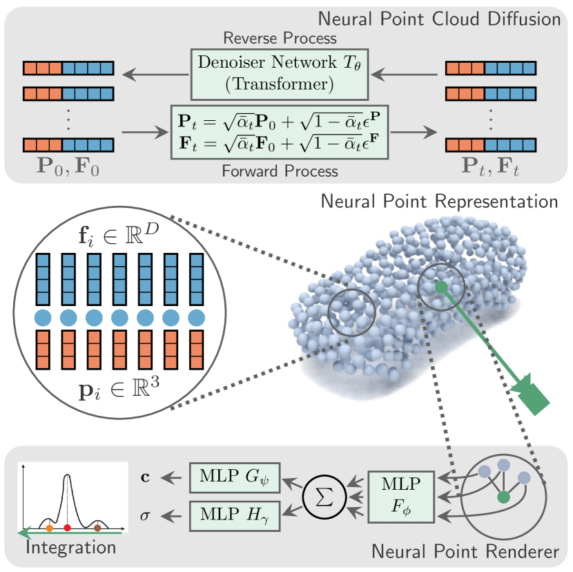
Figure 1: Overview of neural point cloud diffusion (NCPD). In the center we have a neural point cloud representation, where each point has a position ($\blacksquare$) and an appearance feature ($\blacksquare$). The neural point cloud can be generated with a diffusion model (top) and can be rendered via ray integration (bottom).

3.1 Generalizable Point-NeRF

We begin by outlining our representation as an extension of Point-NeRF [42]. A single object is represented by a neural point cloud $\mathcal{P}=\{(\mathbf{p}_{1},\mathbf{f}_{1}),...,(\mathbf{p}_{M},\mathbf{f}_{M})\}=(\mathbf{P},\mathbf{F})$ where each 3D point $i\in\{1,...,M\}$ with position $\mathbf{p}_{i}\in\mathbb{R}^{3}$ is associated with a neural feature $\mathbf{f}_{i}\in\mathbb{R}^{D}$. We denote the full matrix of point positions as $\mathbf{P}\in\mathbb{R}^{M\times 3}$ and the full matrix of features as $\mathbf{F}\in\mathbb{R}^{M\times D}$. In contrast to PointNeRF, we assume the point positions $\mathbf{P}$ to be given for training objects and $\mathbf{F}$ to be manually initialized before optimization. We explore different initialization strategies in Sec. 4.6. The neural point representation can be rendered from arbitrary views, as described in the following.

Volume rendering.

To render a pixel of an image we follow the Point-NeRF [42] procedure. Given camera parameters, we march rays through the scene and sample shading points $\mathbf{q}$ along the ray. For each shading point, the features $\mathbf{f}$ of the neighboring points $\mathbf{p}$ of the neural point cloud are first aggregated to a shading point feature $\mathbf{f}_{\mathbf{q}}$ via a multi-layer perceptron (MLP) $F_{\phi}$ and a weighted combination based on inverse distances:

$$\mathbf{f}_{\mathbf{q}}=\sum\limits_{i=1}\frac{w_{i}F_{\phi}(\mathbf{f}_{i},\mathbf{q}-\mathbf{p}_{i})}{\sum\limits_{i=1}w_{i}},\text{where }w_{i}=\frac{1}{||\mathbf{q}-\mathbf{p}_{i}||_{2}}.$$ (1)

This feature is then mapped mapped to a color $\mathbf{c}$ and density $\sigma$ by separate MLPs $H_{\gamma}$ and $G_{\psi}$:

$$\mathbf{c}=G_{\psi}(\mathbf{f}_{\mathbf{q}})\qquad\sigma=H_{\gamma}(\mathbf{f}_{\mathbf{q}})$$ (2)

The obtained radiances are then numerically integrated to the pixel color as described in NeRF [24]. Given camera parameters $\mathbf{v}$, we denote the full rendering function that renders an image as $R^{\mathbf{v}}_{\phi,\psi,\gamma}(\mathbf{P},\mathbf{F})$.

Optimization.

Optimization is done on a dataset of $N$ objects $O_{1},...,O_{N}$. Each object $O_{j}$ consists of a neural point cloud $\mathcal{P}_{j}=(\mathbf{P}_{j},\mathbf{F}_{j})$ and $K$ views $V_{j1},...,V_{jK}$. Each view $V_{jk}=(\mathbf{I}_{jk},\mathbf{v}_{jk})$ consists of a ground truth image $\mathbf{I}_{jk}$ and corresponding camera parameters $\mathbf{v}_{jk}$. The optimization objective is to jointly find the point features $\mathbf{F}$ and network parameters $\phi,\psi,\gamma$ that minimize the image reconstruction error for all views of all objects:

$$\hat{\mathbf{F}},\textasciiacute\hat{\phi},\textasciiacute\hat{\psi},\hat{\gamma}=\operatorname*{arg\,min}_{\mathbf{F},\textasciiacute\phi,\psi,\gamma}\sum_{j,k}\mathcal{L}\left(R^{\mathbf{v}_{jk}}_{\phi,\psi,\gamma}(\mathbf{P}_{j},\mathbf{F}_{j}),\mathbf{I}_{jk}\right)\textnormal{,}$$ (3)

with $\mathcal{L}$ being the mean squared error between rendered and ground truth pixel colors. In contrast to Point-NeRF, we share parameters $\phi,\psi,\gamma$ of the rendering MLPs over all objects, obtaining a generalizable representation.

3.2 Autodecoding for diffusion

The objective given above in Eq. 3 describes an underconstrained optimization problem. We found that, without further regularization, many-to-one mappings between features $\mathbf{F}$ and renderings $R^{\mathbf{v}}_{\theta,\psi,\phi}(\mathbf{P},\mathbf{F})$ emerge. Thus, there are multiple possible point features $\mathbf{f}_{i}$ representing the same local appearance information. We support this hypothesis with an empirical verification in Sec. 4.6 and Tab. 4. The many-to-one mappings pose a challenge for the denoising model, as it is trained to produce point estimates of the features $\mathbf{f}_{i}$ that are in that case ambiguous.

Most existing latent diffusion methods circumvent this issue by using an autoencoder [32, 45] instead of optimizing representations via backpropagation. Since encoder networks are functions by design, and thus assigning each input value only one output, they do not produce many-to-one mappings between latent representation and output. However, we argue that the autodecoder principle is preferred in many situations, since it does not require an encoder (which is difficult to design for representations like neural points) and often leads to higher quality.

Therefore, we present and analyze a list of strategies to eliminate many-to-one mappings from autodecoder formulations, which are outlined in the following paragraphs.

Zero initialization.

The first simple, albeit effective strategy is to initialize features $\mathbf{F}$ with zero instead of randomly sampled values. We can show that this is very effective and encourages convergence to the same minimum.

Total variation regularization (TV).

Inspired by TV regularization on triplanes [35], we design a TV regularization baseline for our neural point clouds by adding

$$\mathcal{L}_{TV}(\mathbf{F})=\lambda_{TV}\sum_{i=1}^{M}\sum_{n\in\mathcal{V}(i)}\frac{\left\lVert\mathbf{f}_{i}-\mathbf{f}_{n}\right\rVert_{1}}{\left\lVert\mathbf{p}_{i}-\mathbf{p}_{n}\right\rVert_{2}}\,,$$ (4)

with weighting $\lambda_{TV}$ to the objective in Eq. 3 for each object, where $\mathcal{V}(i)$ is a local neigborhood of points around the point with index $i$. Intuitively, it encourages that neighboring point features are varying only slightly.

Variational autodecoder (KL).

We introduce a variational autodecoder by storing vectors of means $\mathbf{\mu}_{i}$ and isotropic variances $\mathbf{\Sigma}_{i}$ instead of features $\mathbf{f}_{i}$ for each point. For rendering, we obtain the features $\mathbf{f}_{i}$ by sampling from the corresponding Gaussians using the reparameterization trick [18]. Additionally, we add a KL divergence loss

$$\mathcal{L}_{KL}(\{\mu_{i},\mathbf{\Sigma}_{i}\}_{i=1}^{M})=\lambda_{KL}\sum_{i=1}^{M}KL(\mathcal{N}(\mathbf{\mu}_{i},\mathbf{\Sigma}_{i}),\mathcal{N}(\mathbf{0},\mathbf{I}_{D}))\,,$$ (5)

for each object with weighting $\lambda_{KL}$, to minimize the evidence lower bound [18]. Intuitively, the consequences from this regularization are twofold. First, the latent space is regularized to follow a unit Gaussian distribution, reducing many-to-one mappings in the representation. Second, the decoder learns to be more robust to small changes in $\mathbf{f}$ due to the sampling procedure. Note that our diffusion model regresses $\mathbf{\mu}_{i}$, but we write $\mathbf{f}_{i}$ in the following for simplicity.

3.3 Neural point cloud diffusion

In this section, we describe our diffusion model for neural point cloud representations. As input, we assume a set of optimized representations $\{\mathcal{P}_{j}\}_{j=1}^{N}$ from the first stage. The diffusion model learns the distribution of these representations, which allows us to generate neural point clouds.

Denoising diffusion background.

Diffusion models [37, 38] learn the distribution $q(\mathbf{x})$ of data $\mathbf{x}$ by defining a forward diffusion process in form of a Markov chain with steps $q(\mathbf{x}_{t}|\mathbf{x}_{t-1})$ that gradually transform the data distribution into a simple known distribution. A model $p_{\theta}(\mathbf{x}_{t-1}|\mathbf{x}_{t})$ with parameters $\theta$ is then trained to approximate the steps $q(\mathbf{x}_{t-1}|\mathbf{x}_{t})$ in the Markov chain of the reverse process, which allows to evaluate the likelihood of a given data point, or sample from the learnt distribution.

In case of Gaussian diffusion processes, the forward diffusion process gradually replaces the data with Gaussian noise following a noise schedule $\beta_{1},..,\beta_{T}$:

$$q(\mathbf{x}_{t}|\mathbf{x}_{t-1})\coloneqq\mathcal{N}(\mathbf{x}_{t};\sqrt{1-\beta_{t}}\mathbf{x}_{t-1},\beta_{t}\mathbf{I})\,.$$ (6)

Further, it is possible to sample $\mathbf{x}_{t}$ directly from $\mathbf{x}_{0}$:

$$q(\mathbf{x}_{t}|\mathbf{x}_{0})=\mathcal{N}(\mathbf{x}_{t};\sqrt{\bar{\alpha}_{t}}\mathbf{x}_{0},(1-\bar{\alpha}_{t})\mathbf{I})\,,$$ (7)

with $\alpha_{t}\coloneqq 1-\beta_{t}$ and $\bar{\alpha}_{t}\coloneqq\prod_{s=1}^{t}\alpha_{s}$. For small enough step sizes in the noise schedule, the steps in the Markov chain of the reverse process can be approximated with Gaussian distributions:

$$p_{\theta}(\mathbf{x_{T}}) =\mathcal{N}(\mathbf{x}_{T};\mathbf{0},\mathbf{I}),$$ (8)

$$p_{\theta}(\mathbf{x}_{t-1}|\mathbf{x}_{t}) =\mathcal{N}(\mathbf{x}_{t-1};\mu_{\theta}(\mathbf{x}_{t},t),\Sigma_{\theta}(\mathbf{x}_{t},t))\,.$$ (9)

The objective hence is to learn $\mu_{\theta}(\mathbf{x}_{t},t)$ and $\Sigma_{\theta}(\mathbf{x}_{t},t)$. DDPM [13] proposes a diffusion model formulation with various simplifications. Specifically, DDPM suggests to fix $\Sigma_{\theta}(\mathbf{x}_{t},t)$ and the noise schedule $\beta_{t}$ to time-dependent constants. Further, DDPM reparametrizes Eq. 7 to

$$\mathbf{x}_{t}(\mathbf{x}_{0},\mathbf{\epsilon})=\sqrt{\bar{\alpha}_{t}}\mathbf{x}_{0}+\sqrt{1-\bar{\alpha}_{t}}\mathbf{\epsilon}\text{ with }\mathbf{\epsilon}\sim\mathcal{N}(\mathbf{0},\mathbf{I})$$ (10)

and trains the model to directly predict $\mathbf{\epsilon}_{\theta}(\mathbf{x}_{t},t)$, from which $\mu_{\theta}(\mathbf{x}_{t},t)$ can be computed.

Neural point cloud diffusion.

Given the background in DDPM, we turn to describing our neural point cloud diffusion. Conceptually, the neural points clouds $\mathcal{P}=(\mathbf{P},\mathbf{F})$ take the place of data points $\mathbf{x}_{0}$ in the above DDPM diffusion model formulation.

The distribution of both modalities, point positions $\mathbf{P}$ and appearance features $\mathbf{F}$, is learnt jointly. During training, we sample Gaussian noise $\mathbf{\epsilon}^{\mathbf{P}}$ for all point positions and $\mathbf{\epsilon}^{\mathbf{F}}$ for all point features and use it to obtain the noised neural point cloud $\mathcal{P}_{t}=(\mathbf{P}_{t},\mathbf{F}_{t})$ at a specific timestep $t$ in the diffusion process via Eq. 10. The denoiser network $T_{\theta}((\mathbf{P}_{t},\mathbf{F}_{t}),t)=(\mathbf{\epsilon}^{\mathbf{P}}_{\theta},\mathbf{\epsilon}^{\mathbf{F}}_{\theta})$ takes the noised neural point cloud and timestep as input and estimates the noise $\mathbf{\epsilon}^{\mathbf{P}}_{\theta}$ and $\mathbf{\epsilon}^{\mathbf{F}}_{\theta}$ that was applied to the points and features. The network is optimized by minimizing the average mean squared error on both noise vectors:

$$\mathcal{L}_{T}=\frac{1}{2}(\text{MSE}(\mathbf{\epsilon}^{\mathbf{P}},\mathbf{\epsilon}^{\mathbf{P}}_{\theta})+\text{MSE}(\mathbf{\epsilon}^{\mathbf{F}},\mathbf{\epsilon}^{\mathbf{F}}_{\theta}))\,.$$ (11)

Denoiser architecture.

As the architecture for the denoiser network we use a Transformer [26, 40]. As input, the transformer receives $M+1$ tokens, one token per point plus one additional token encoding $t$. Point tokens are obtained by concatenating the point position and feature of each point in the noisy point cloud and projecting them with a linear layer. Similarly, the $t$ token is obtained by projection with its own linear layer onto the same dimensionality. After encoding, all tokens are processed by transformer layers, including self-attention and MLPs. Finally, the resulting output tokens corresponding to the $M$ points are projected back to the dimensions of the input point positions and features and interpreted as noise predictions $\mathbf{\epsilon}^{\mathbf{P}}_{\theta}$ and $\mathbf{\epsilon}^{\mathbf{F}}_{\theta}$.

3.4 Disentangled generation

Given a trained NPCD model, we can naively sample from the joint distribution $p(\mathbf{P},\mathbf{F})$ of point positions and features by sampling positions and features from a unit Gaussian distribution and using the transformer for iterative denoising (c.f. LABEL:fig:teaser for a visualization). To achieve individual generation of shape and appearance, one needs to sample from conditional distributions $p(\mathbf{P}|\mathbf{F})$ or $p(\mathbf{F}|\mathbf{P})$ instead.

To sample from $p(\mathbf{F}|\mathbf{P})$ given point positions $\mathbf{P}_{0}$, we obtain the initial noisy neural point cloud $\mathcal{P}_{T}=(\mathbf{P}_{T},\mathbf{F}_{T})$ by

$$\mathbf{P}_{T}=\sqrt{\bar{\alpha}_{t}}\mathbf{P}_{0}+\sqrt{1-\bar{\alpha}_{t}}\mathbf{\epsilon}^{\mathbf{P}},\quad\mathbf{F}_{T}\sim\mathcal{N}(\mathbf{0},\mathbf{I})\textnormal{,}$$ (12)

i.e., only sampling $\mathbf{F}_{T}$ from noise while obtaining $\mathbf{P}_{T}$ as a noisy variant of $\mathbf{P}_{0}$. Then, the denoising transformer is applied. After each reverse process iteration, we reset $\mathbf{P}_{t}$ to the values from Eq. 12 for the appropriate $t$. Sampling from $p(\mathbf{P}|\mathbf{F})$ can be done analogously.

Note that the conditional sampling procedure described above is enabled by the neural point representations, which allow to individually modify the disentangled variables for coarse shape and local appearance.

4 Experiments

In this section, we provide experimental results for the presented NPCD method. We begin by introducing the experimental setup in Sec. 4.1 and used metrics in Sec. 4.2. Then, we evaluate the main contribution of our method in Sec. 4.3, i.e. the distentangled generation of coarse geometry and appearance. We compare against previous generative approaches that allow disentangled generation, namely GRAF [34] and Disentangled3D [39], and show our superior generation quality. Next, we compare against recent diffusion models without disentangling capabilities in Sec. 4.4. Here, we compare against DiffRF [25], Functa [10] and SSDNeRF [8]. Many existing 3D generative models model only shape but not appearance. Thus, to complement existing comparisons, we also provide a shape-only comparison in Sec. 4.5. Finally, we analyze many-to-one mappings due to auto-decoded features as a problem for diffusion models and propose regularization methods as effective countermeasures in Sec. 4.6.

4.1 Datasets and experimental setup

Data.

We use the cars and chairs categories of the ShapeNet SRN dataset [7, 36]. The cars split contains $2{,}458$ training objects and $704$ test objects, while the chairs split contains $4{,}611$ training and $1{,}317$ test objects. We use the original renderings with 50 views per training object and 251 views per test object. The images have a resolution of 128x128 pixels. For all training objects, the poses are sampled randomly from a sphere. For all test objects the poses follow a spiral on the upper hemisphere. We extract point clouds with 30k points from the mesh and subsample them to 512 points with farthest point sampling.

Besides ShapeNet SRN, we also use the PhotoShape Chairs dataset [29]. The dataset contains $15{,}576$ objects and features more realistic textures on top of ShapeNet meshes. We use the same test split as DiffRF [25], which consists of $1,552$ objects. From the remaining objects, we randomly select $2,480$ objects for training. Further, we use the same renderings as DiffRF [25], which consist of 200 views per object on an Archimedean spiral. We use images at a resolution of 128x128 pixels. We use the same point clouds with 512 points as for SRN chairs.

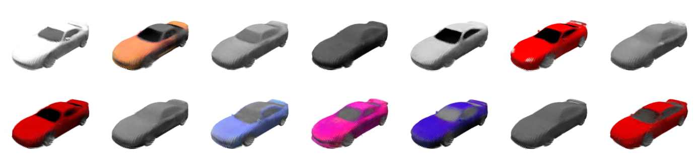
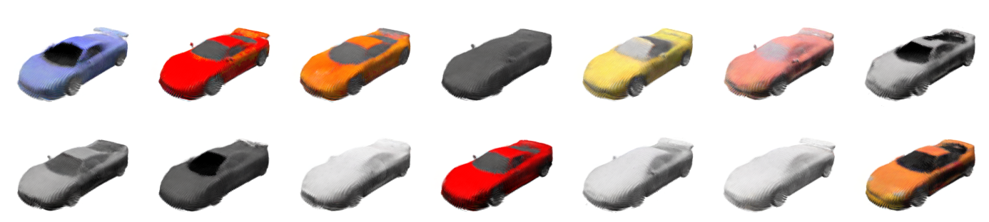
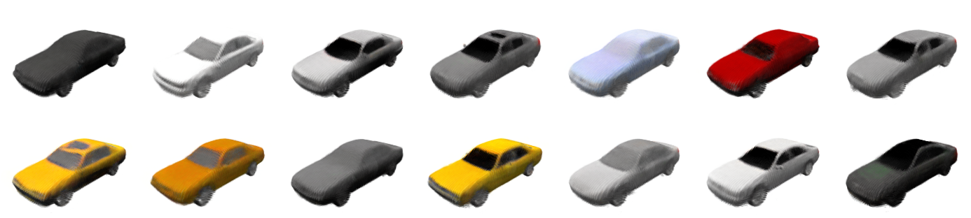
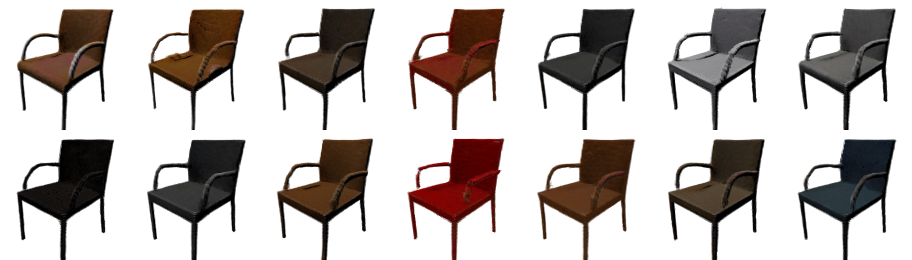
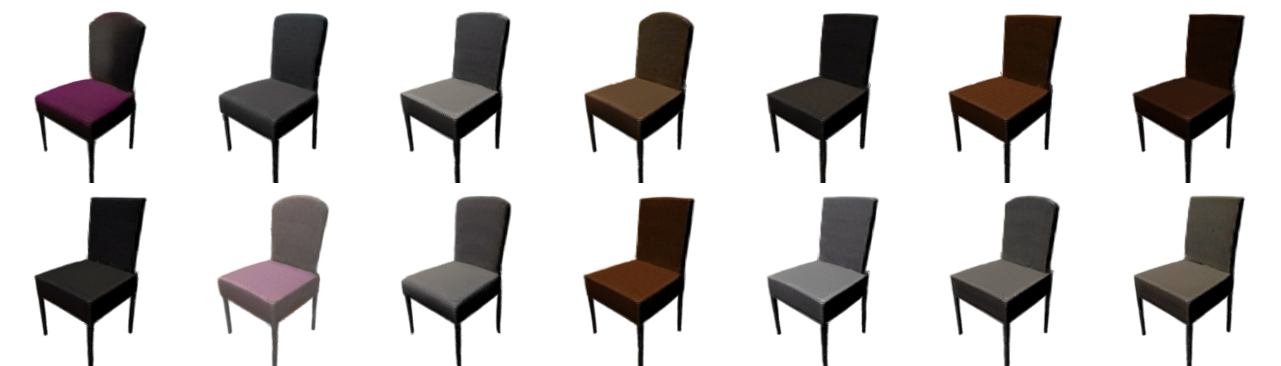
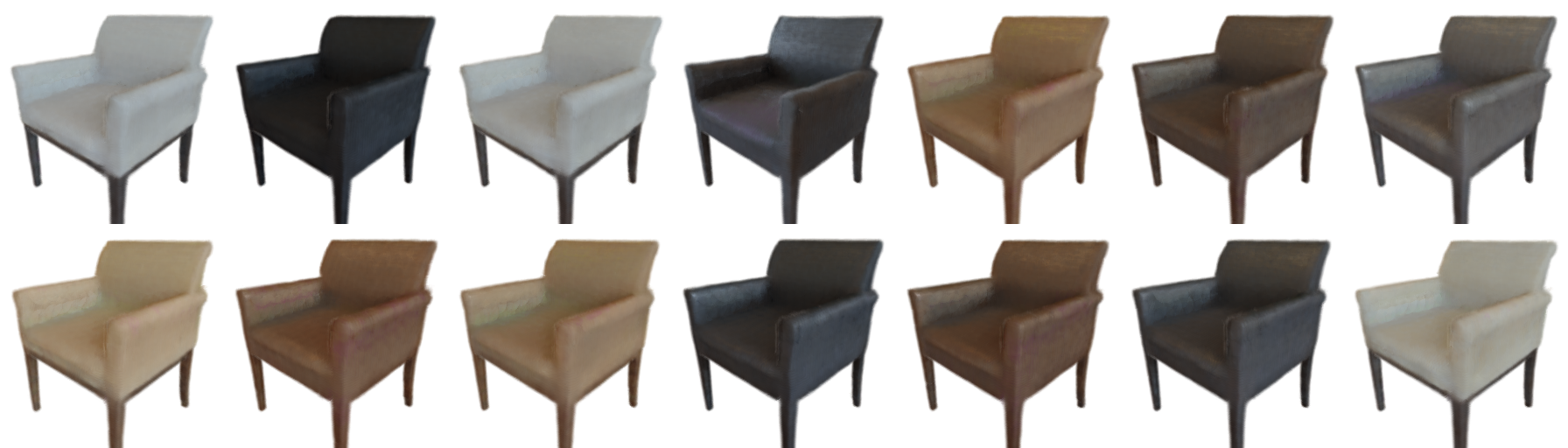
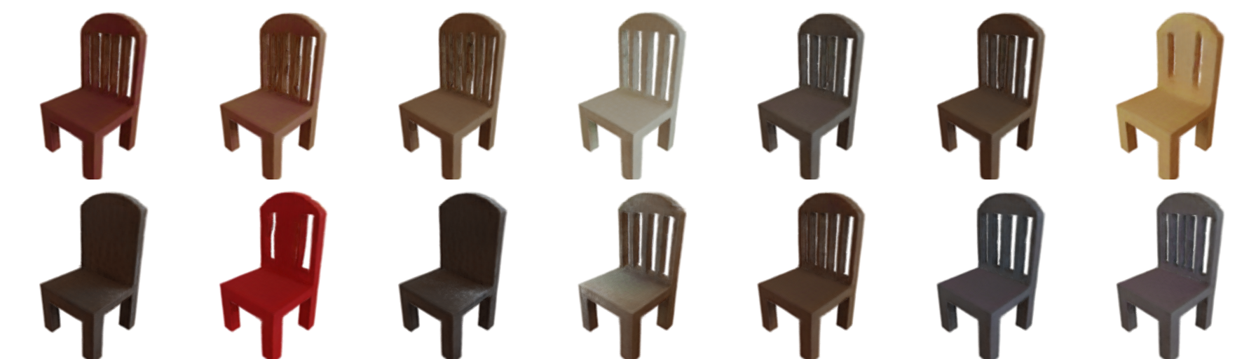
(a)

Figure 2: Qualitative examples of disentangled generation on SRN cars, SRN chairs, PhotoShape chairs. 2(a) Appearance-only generation: we show a generated object and objects with re-sampled appearance. 2(b) Shape-only generation: we show a generated object and objects with re-sampled coarse shape. We can get diverse samples of local appearance or coarse shape when the respective other is given.

 

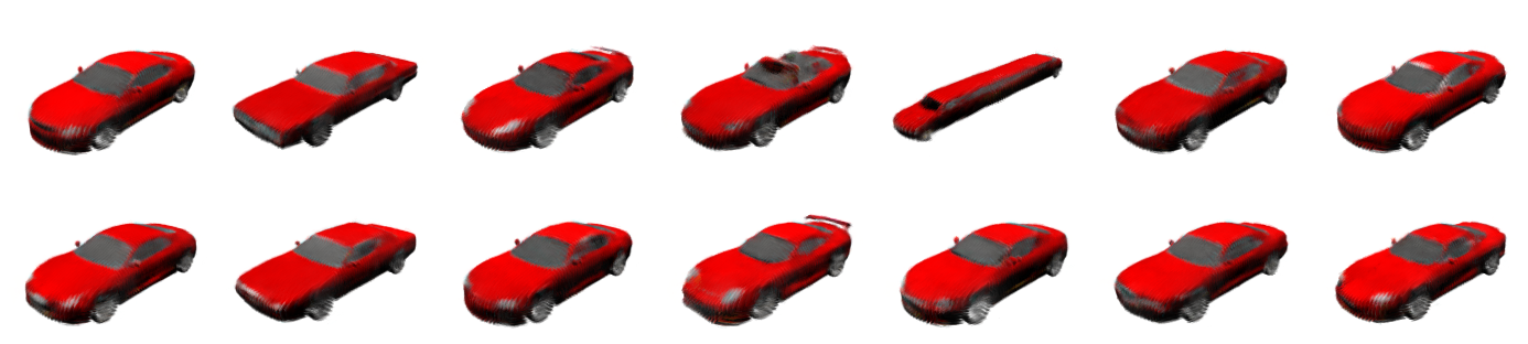
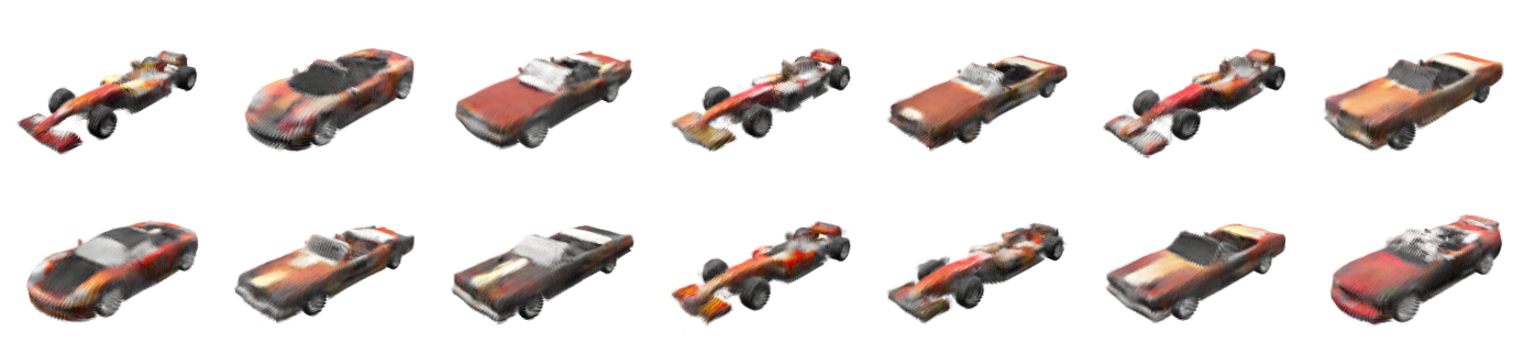
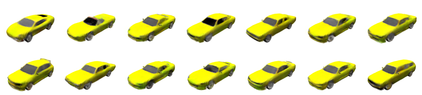
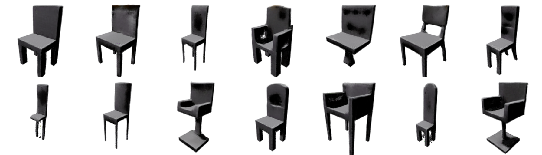
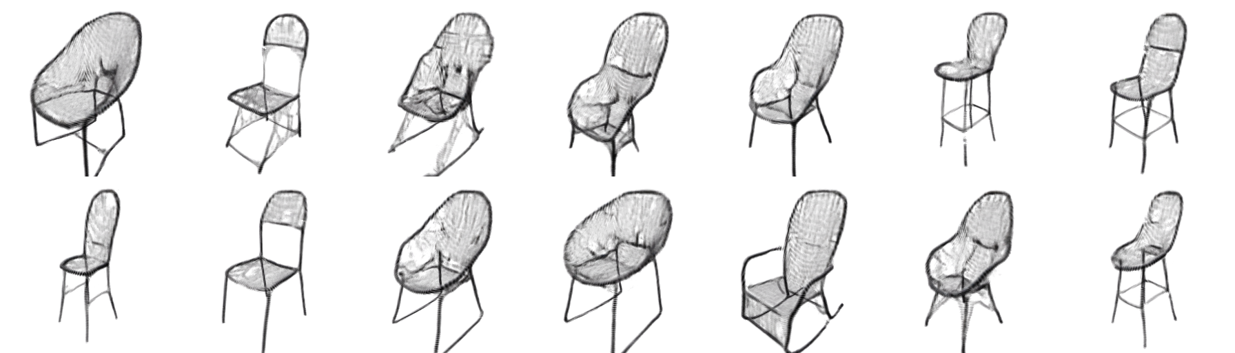
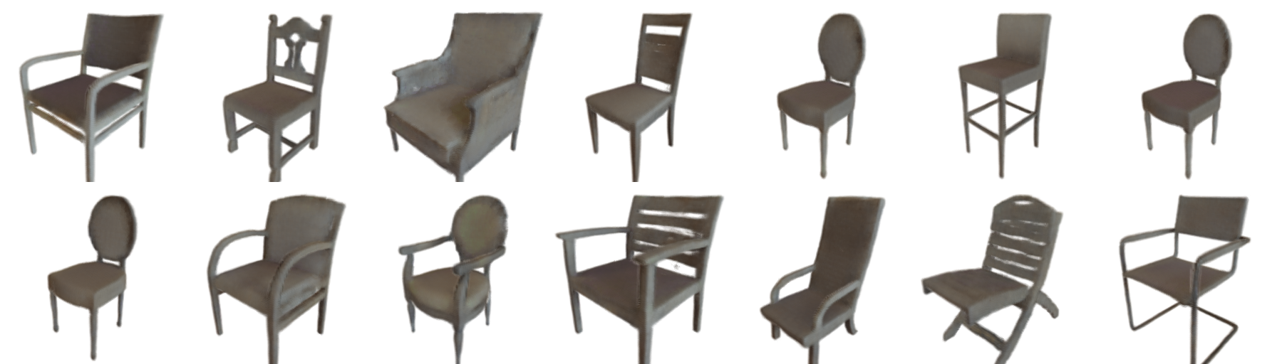
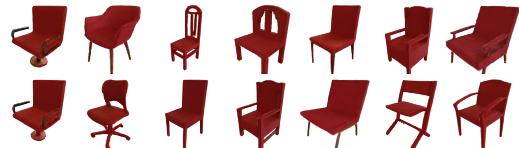
(b)

Training details.

We construct neural point clouds by zero-initializing features for each point. In generalizable Point-NeRF, we optimize the reconstruction loss in Eq. 3 with the TV and KL regularizers from Eq. 4 and Eq. 5. Further details on network architectures and training parameters are provided in the supplementals. For the diffusion model training, we normalize the neural point clouds and use DDPM [13] diffusion model parameters. Further details on the denoiser architecture, diffusion model parameters, and training parameters are provided in the supplementals.

4.2 Metrics

To measure the quality and diversity of the generated samples of the diffusion model, we report the FID [12] and KID [3] metrics. FID and KID compare the appearance and diversity of two image sets by computing features for each image with an Inception model and comparing the feature distributions of the two sets. We use the images of the test set objects as the reference set. For comparability, we follow the evaluation procedures of previous works: on SRN Cars and Chairs, we generate the same number of objects as in the test set and render them from the same poses; on PhotoShape Chairs, we generate $1{,}000$ objects and render them from 10 poses that are sampled randomly from the Archimedean spiral poses. Furthermore, for the shape-only evaluation of our generated point clouds representing the coarse geometry, we employ 1-nearest-neighbor accuracy w.r.t. Chamfer and Earth Mover’s Distance [43]. Last, we conduct a quantitative analysis by reporting the per-point mean cosine similarities between optimized neural point features of $10$ random training examples over $100$ different seeds with a fixed renderer. This measures the extent of many-to-one mappings, i.e. how far features that represent the same appearance are away from each other.

4.3 Disentangled generation

A major advantage of using neural point clouds as 3D representation is their intrinsic disentanglement of shape and appearance: the point positions represent the coarse geometry and the features model local geometry and appearance. As described in Sec. 3.4, this property enables the proposed method to generate both modalities separately, even though a joint distribution is modeled with a single diffusion model. In the following, we present the results of this disentangled 3D shape and appearance generation.

NPCD allows to explicitly control the point positions or point features throughout the diffusion process. As a consequence, we can re-sample appropriate features that fit to the given point positions or vice versa, resulting in generating new samples with one modality fixed. Results for the appearance-only generation are shown in Fig. 2(a) and for the shape-only generation in Fig. 2(b). It can be seen that our method succeeds in generating diverse novel shapes or appearances when one modality is fixed. Note that our method performs an actual recombination and does more than retrieval of objects from the training dataset.

Previous approaches that are able to generate disentangled 3D shape and appearance are GRAF [34] and Disentangled3D (D3D) [39], which are both GAN-based. We provide a quantitative comparison to these approaches regarding generation quality in Tab. 1 and a qualitative comparison in Fig. 3. Our comparisons show that our proposed method is capable of disentangled generation with superior quality than these previous approaches.

Model	ShapeNet SRN				PhotoShape
	Cars		Chairs		Chairs
	FID$\downarrow$	KID/10−3$\downarrow$	FID$\downarrow$	KID/10−3$\downarrow$	FID$\downarrow$	KID/10−3$\downarrow$
GRAF [34]	40.95	19.15	37.19	17.85	34.49	17.13
D3D [39]	62.34	41.60	45.73	24.33	59.80	36.07
NPCD (Ours)	28.38	17.62	9.87	3.62	14.45	5.40

Table 1: Comparison to disentanglement-capable approaches. The numbers show that we clearly outperform previous generative models that allow disentangled generation.

Cars
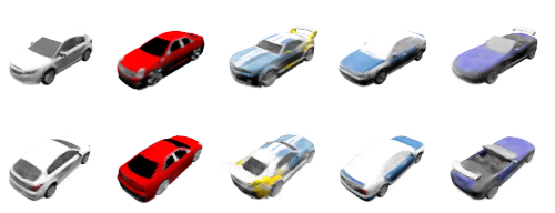
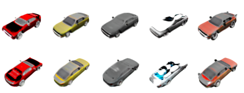
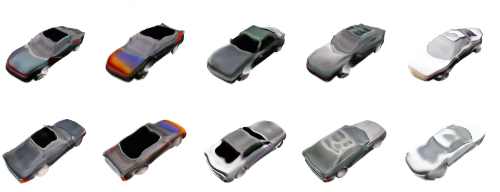
Chairs
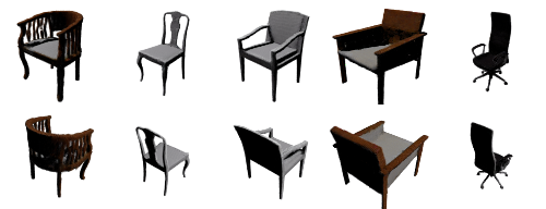
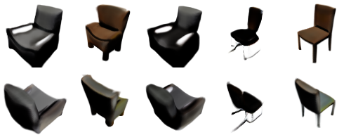
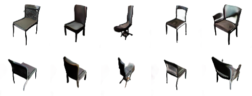
PS Chairs
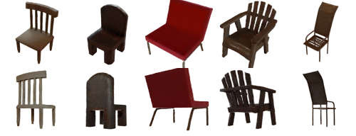
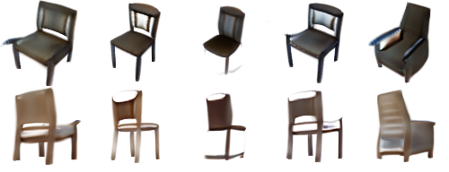
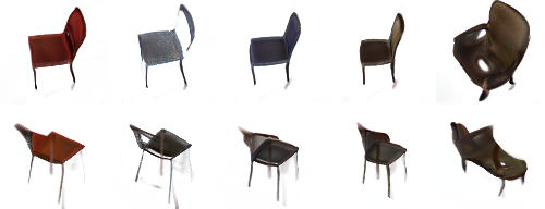
Ours	GRAF [34]	Disentangled3D [39]

Figure 3: Comparison against previous generative models that allow disentangled generation.: While we present the first diffusion model allowing disentangled generation, earlier works are GAN-based. It can be seen that our model generates examples in much higher quality, as also evident from the metrics in Tab. 1.

4.4 3D diffusion comparison

We compare NPCD with Functa [10], SSDNeRF [8], and DiffRF [25], previous works that generate 3D shape and appearance on medium-scale datasets with 3D diffusion models. We compare against SSDNeRF and Functa on SRN Cars and against DiffRF on Photoshape Chairs. Quantitative results are provided in Tab. 2. Our proposed method performs better than Functa and DiffRF methods and worse than SSDNeRF regarding the FID and KID metrics. However, none of these methods enable disentangled generation.

Model	PhotoShape Chairs
	FID$\downarrow$	KID/10−3$\downarrow$
DiffRF	15.95	7.93
NPCD (Ours)	14.45	5.40

Model	SRN Cars
	FID$\downarrow$	KID/10−3$\downarrow$
Functa	80.3	-
SSDNeRF	11.08	3.47
NPCD (Ours)	28.38	17.62

Table 2: Comparison to 3D diffusion models for unconditional 3D shape and appearance generation. Our NPCD model achieves better scores than DiffRF and Functa. SSDNeRF performs slightly better. However, none of the other models enable disentangled generation.

4.5 Shape-only comparison

Since our neural radiance field is build on top of a coarse point cloud, we evaluate the geometry of NPCD samples by comparing with the state of the art in point cloud generation in Tab. 3. Even though the point cloud defines only the coarse structure beneath a fine radiance field, the quality and diversity of our generated point clouds is comparable to the ones from approaches that are specialized for shape-only generation.

Model	SRN Cars		SRN Chairs
	CD$\downarrow$	EMD$\downarrow$	CD$\downarrow$	EMD$\downarrow$
r-GAN [1]	94.46	99.01	83.69	99.70
PointFlow [43]	58.10	56.25	62.84	60.57
SoftFlow [17]	64.77	60.09	59.21	60.05
DPF-Net [19]	62.35	54.48	62.00	58.53
Shape-GF [4]	63.20	56.53	68.96	65.48
PVD [47]	54.55	53.83	56.26	53.32
LION [45]	53.41	51.14	53.70	52.34
NPCD (Ours)	60.23	52.41	60.50	58.84

Table 3: Shape-only comparison. We evaluate the point cloud generation part of our approach individually. Despite being just the coarse structure of a finer radiance field on top, NPCD can compete with the state of the art in point cloud generation.

4.6 Analysis

As diffusion on hybrid point clouds and local radiance fields has not been done before, we conduct ablation studies and analyze various novel design choices. Here, we analyze the effects of different initialization strategies, feature dimensionality and regularization methods in the generalizable Point-NeRF and diffusion model. We provide a more detailed analysis in the supplementals.

Neural point cloud initialization

Regarding the initialization of the neural point cloud features, we analyze initialization with features sampled from a Gaussian distribution against a zero initialization. Interestingly, we find that these different initializations strongly affect the feature space of the trained models, which directly translates to differences in generation quality (c.f. supplementals). Tab. 4 indicates that the simple measure of zero initialization is able to largely mitigate the many-to-one mappings in the MLP decoder and provide much more coherent features.

Neural point cloud regularization

As we assume that the structure of the feature space strongly affects the diffusion model, we analyze the effects of applying KL and TV regularizations to the neural point features during the generalizable Point-NeRF training. Tab. 4 shows that both regularizations further decrease the ambiguity of the latent space over the zero initialization. We can summarize that a combination of TV and KL regularization provides overall the best results (c.f. supplementals). Overall, we found an appropriate initialization and regularization to be key ingredients for successful neural point cloud diffusion.

Init.	Reg.	$\lambda$	Cosine sim.
Rand.	✗	-	0.0306
Zero	✗	-	0.7695
Zero	TV	3.5e-6	0.9355
Zero	KL	1e-6	0.9480
Zero	TV,KL	3e-7,1e-7	0.9470

Table 4: Auto-decoded feature similarity. We compute per-point mean cosine similarities between optimized neural point features of $10$ training examples for $100$ different seeds. Zero initialization and regularization effectively reduce the ambiguity of the auto-decoded latent space. This improves generation quality significantly, as shown in the supplementals.

5 Conclusion

We presented a diffusion approach for neural point clouds with high-dimensional features that represent local parts of objects and can be rendered to images. We have shown that, in contrast to all other current 3D diffusion models, the neural point cloud enables our method to effectively disentangle the coarse shape from the fine geometry and appearance and to control both factors separately. In experiments on ShapeNet and PhotoShape we could show that we clearly outperform previous methods that perform disentangled generation of 3D objects, while being competitive with unconditional generation methods. Further, we provide an extensive analysis and identified many-to-one mappings in auto-decoded latent spaces as the main challenge for the successful training of a latent diffusion model. Therefore, we proposed a suitable initialization and regularization of the neural point features as effective countermeasures.

See pages 1 of ./001_supplementary.pdf See pages 2 of ./001_supplementary.pdf See pages 3 of ./001_supplementary.pdf See pages 4 of ./001_supplementary.pdf See pages 5 of ./001_supplementary.pdf See pages 6 of ./001_supplementary.pdf See pages 7 of ./001_supplementary.pdf See pages 8 of ./001_supplementary.pdf

References

- Achlioptas et al. [2018] Panos Achlioptas, Olga Diamanti, Ioannis Mitliagkas, and Leonidas Guibas. Learning representations and generative models for 3D point clouds. In ICML, 2018.
- Anciukevičius et al. [2023] Titas Anciukevičius, Zexiang Xu, Matthew Fisher, Paul Henderson, Hakan Bilen, Niloy J. Mitra, and Paul Guerrero. Renderdiffusion: Image diffusion for 3d reconstruction, inpainting and generation. In CVPR, 2023.
- Bińkowski et al. [2018] Mikołaj Bińkowski, Danica J. Sutherland, Michael Arbel, and Arthur Gretton. Demystifying mmd gans. In ICLR, 2018.
- Cai et al. [2020] Ruojin Cai, Guandao Yang, Hadar Averbuch-Elor, Zekun Hao, Serge Belongie, Noah Snavely, and Bharath Hariharan. Learning gradient fields for shape generation. In ECCV, 2020.
- Chabra et al. [2020] Rohan Chabra, Jan E. Lenssen, Eddy Ilg, Tanner Schmidt, Julian Straub, Steven Lovegrove, and Richard Newcombe. Deep local shapes: Learning local SDF priors for detailed 3D reconstruction. In ECCV, 2020.
- Chan et al. [2022] Eric R. Chan, Connor Z. Lin, Matthew A. Chan, Koki Nagano, Boxiao Pan, Shalini De Mello, Orazio Gallo, Leonidas Guibas, Jonathan Tremblay, Sameh Khamis, Tero Karras, and Gordon Wetzstein. Efficient geometry-aware 3D generative adversarial networks. In CVPR, 2022.
- Chang et al. [2015] Angel X. Chang, Thomas Funkhouser, Leonidas Guibas, Pat Hanrahan, Qixing Huang, Zimo Li, Silvio Savarese, Manolis Savva, Shuran Song, Hao Su, Jianxiong Xiao, Li Yi, and Fisher Yu. ShapeNet: An information-rich 3d model repository. Technical Report arXiv:1512.03012, Stanford University — Princeton University — Toyota Technological Institute at Chicago, 2015.
- Chen et al. [2023] Hansheng Chen, Jiatao Gu, Anpei Chen, Wei Tian, Zhuowen Tu, Lingjie Liu, and Hao Su. Single-stage diffusion nerf: A unified approach to 3d generation and reconstruction, 2023.
- Dhariwal and Nichol [2021] Prafulla Dhariwal and Alexander Nichol. Diffusion models beat gans on image synthesis. In NeurIPS, 2021.
- Dupont et al. [2022] Emilien Dupont, Hyunjik Kim, S. M. Ali Eslami, Danilo Jimenez Rezende, and Dan Rosenbaum. From data to functa: Your data point is a function and you can treat it like one. In ICML, 2022.
- Erkoç et al. [2023] Ziya Erkoç, Fangchang Ma, Qi Shan, Matthias Nießner, and Angela Dai. HyperDiffusion: Generating implicit neural fields with weight-space diffusion, 2023.
- Heusel et al. [2017] Martin Heusel, Hubert Ramsauer, Thomas Unterthiner, Bernhard Nessler, and Sepp Hochreiter. Gans trained by a two time-scale update rule converge to a local nash equilibrium. In NeurIPS, 2017.
- Ho et al. [2020] Jonathan Ho, Ajay Jain, and Pieter Abbeel. Denoising diffusion probabilistic models. In NeurIPS, 2020.
- Jang and Agapito [2021] Wonbong Jang and Lourdes Agapito. Codenerf: Disentangled neural radiance fields for object categories. In ICCV, 2021.
- Jun and Nichol [2023] Heewoo Jun and Alex Nichol. Shap-E: Generating conditional 3d implicit functions. arXiv:2305.02463, 2023.
- Karras et al. [2022] Tero Karras, Miika Aittala, Timo Aila, and Samuli Laine. Elucidating the design space of diffusion-based generative models. In NeurIPS, 2022.
- Kim et al. [2020] Hyeongju Kim, Hyeonseung Lee, Woo Hyun Kang, Joun Yeop Lee, and Nam Soo Kim. Softflow: Probabilistic framework for normalizing flow on manifolds. In NeurIPS, 2020.
- Kingma and Welling [2014] Diederik P. Kingma and Max Welling. Auto-Encoding Variational Bayes. In ICLR, 2014.
- Klokov et al. [2020] Roman Klokov, Edmond Boyer, and Jakob Verbeek. Discrete point flow networks for efficient point cloud generation. In ECCV, 2020.
- Lin et al. [2023] Chen-Hsuan Lin, Jun Gao, Luming Tang, Towaki Takikawa, Xiaohui Zeng, Xun Huang, Karsten Kreis, Sanja Fidler, Ming-Yu Liu, and Tsung-Yi Lin. Magic3d: High-resolution text-to-3d content creation. In CVPR, 2023.
- Liu et al. [2023] Ruoshi Liu, Rundi Wu, Basile Van Hoorick, Pavel Tokmakov, Sergey Zakharov, and Carl Vondrick. Zero-1-to-3: Zero-shot one image to 3d object. arXiv preprint arXiv:2303.11328, 2023.
- Luo and Hu [2021] Shitong Luo and Wei Hu. Diffusion probabilistic models for 3d point cloud generation. In CVPR, 2021.
- Melas-Kyriazi et al. [2023] Luke Melas-Kyriazi, Iro Laina, Christian Rupprecht, and Andrea Vedaldi. Realfusion: 360deg reconstruction of any object from a single image. In CVPR, 2023.
- Mildenhall et al. [2020] Ben Mildenhall, Pratul P. Srinivasan, Matthew Tancik, Jonathan T. Barron, Ravi Ramamoorthi, and Ren Ng. Nerf: Representing scenes as neural radiance fields for view synthesis. In ECCV, 2020.
- Müller et al. [2023] Norman Müller, Yawar Siddiqui, Lorenzo Porzi, Samuel Rota Bulo, Peter Kontschieder, and Matthias Nießner. Diffrf: Rendering-guided 3d radiance field diffusion. In CVPR, 2023.
- Nichol et al. [2022] Alex Nichol, Heewoo Jun, Prafulla Dhariwal, Pamela Mishkin, and Mark Chen. Point-E: A system for generating 3d point clouds from complex prompts. arXiv:2212.08751, 2022.
- Niemeyer and Geiger [2021] Michael Niemeyer and Andreas Geiger. Giraffe: Representing scenes as compositional generative neural feature fields. In CVPR, 2021.
- Niemeyer et al. [2020] Michael Niemeyer, Lars Mescheder, Michael Oechsle, and Andreas Geiger. Differentiable volumetric rendering: Learning implicit 3d representations without 3d supervision. In CVPR, 2020.
- Park et al. [2018] Keunhong Park, Konstantinos Rematas, Ali Farhadi, and Steven M. Seitz. Photoshape: Photorealistic materials for large-scale shape collections. ACM TOG, 2018.
- Poole et al. [2023] Ben Poole, Ajay Jain, Jonathan T. Barron, and Ben Mildenhall. Dreamfusion: Text-to-3d using 2d diffusion. In ICLR, 2023.
- Ramesh et al. [2021] Aditya Ramesh, Mikhail Pavlov, Gabriel Goh, Scott Gray, Chelsea Voss, Alec Radford, Mark Chen, and Ilya Sutskever. Zero-shot text-to-image generation. In ICML, 2021.
- Rombach et al. [2022] Robin Rombach, Andreas Blattmann, Dominik Lorenz, Patrick Esser, and Björn Ommer. High-resolution image synthesis with latent diffusion models. In CVPR, 2022.
- Saharia et al. [2022] Chitwan Saharia, William Chan, Saurabh Saxena, Lala Li, Jay Whang, Emily L Denton, Kamyar Ghasemipour, Raphael Gontijo Lopes, Burcu Karagol Ayan, Tim Salimans, et al. Photorealistic text-to-image diffusion models with deep language understanding. In NeurIPS, 2022.
- Schwarz et al. [2020] Katja Schwarz, Yiyi Liao, Michael Niemeyer, and Andreas Geiger. Graf: Generative radiance fields for 3d-aware image synthesis. In NeurIPS, 2020.
- Shue et al. [2023] J. Ryan Shue, Eric Ryan Chan, Ryan Po, Zachary Ankner, Jiajun Wu, and Gordon Wetzstein. 3d neural field generation using triplane diffusion. In CVPR, 2023.
- Sitzmann et al. [2019] Vincent Sitzmann, Michael Zollhöfer, and Gordon Wetzstein. Scene representation networks: Continuous 3d-structure-aware neural scene representations. In NeurIPS, 2019.
- Sohl-Dickstein et al. [2015] Jascha Sohl-Dickstein, Eric Weiss, Niru Maheswaranathan, and Surya Ganguli. Deep unsupervised learning using nonequilibrium thermodynamics. In ICML, 2015.
- Song and Ermon [2019] Yang Song and Stefano Ermon. Generative modeling by estimating gradients of the data distribution. In NeurIPS, 2019.
- Tewari et al. [2022] Ayush Tewari, MalliKarjun B R, Xingang Pan, Ohad Fried, Maneesh Agrawala, and Christian Theobalt. Disentangled3d: Learning a 3d generative model with disentangled geometry and appearance from monocular images. In CVPR, 2022.
- Vaswani et al. [2017] Ashish Vaswani, Noam Shazeer, Niki Parmar, Jakob Uszkoreit, Llion Jones, Aidan N Gomez, Ł ukasz Kaiser, and Illia Polosukhin. Attention is all you need. In NeurIPS, 2017.
- Wewer et al. [2023] Christopher Wewer, Eddy Ilg, Bernt Schiele, and Jan Eric Lenssen. Simnp: Learning self-similarity priors between neural points. In ICCV, 2023.
- Xu et al. [2022] Qiangeng Xu, Zexiang Xu, Julien Philip, Sai Bi, Zhixin Shu, Kalyan Sunkavalli, and Ulrich Neumann. Point-NeRF: Point-based neural radiance fields. In CVPR, 2022.
- Yang et al. [2019] Guandao Yang, Xun Huang, Zekun Hao, Ming-Yu Liu, Serge Belongie, and Bharath Hariharan. Pointflow: 3d point cloud generation with continuous normalizing flows. In ICCV, 2019.
- Yao et al. [2018] Yao Yao, Zixin Luo, Shiwei Li, Tian Fang, and Long Quan. Mvsnet: Depth inference for unstructured multi-view stereo. In ECCV, 2018.
- Zeng et al. [2022] Xiaohui Zeng, Arash Vahdat, Francis Williams, Zan Gojcic, Or Litany, Sanja Fidler, and Karsten Kreis. LION: Latent point diffusion models for 3d shape generation. In NeurIPS, 2022.
- Zhang and Agrawala [2023] Lvmin Zhang and Maneesh Agrawala. Adding conditional control to text-to-image diffusion models. arXiv preprint arXiv:2302.05543, 2023.
- Zhou et al. [2021] Linqi Zhou, Yilun Du, and Jiajun Wu. 3d shape generation and completion through point-voxel diffusion. In ICCV, 2021.
- Zhou and Tulsiani [2023] Zhizhuo Zhou and Shubham Tulsiani. Sparsefusion: Distilling view-conditioned diffusion for 3d reconstruction. In CVPR, 2023.
- Zhu et al. [2018] Jun-Yan Zhu, Zhoutong Zhang, Chengkai Zhang, Jiajun Wu, Antonio Torralba, Josh Tenenbaum, and Bill Freeman. Visual object networks: Image generation with disentangled 3d representations. In NeurIPS, 2018.