Neutrino masses from new seesaw models: Low-scale variants and phenomenological implications

Abstract

With just the Standard Model Higgs doublet, there are only three types of seesaw models that generate light Majorana neutrino masses at tree level after electroweak spontaneous symmetry breaking. However, if there exist additional TeV scalars acquiring vacuum expectation values, coupled with heavier fermionic multiplets, several new seesaw models become possible. These new seesaws are the primary focus of this study and correspond to the tree-level ultraviolet completions of the effective operators studied in a companion publication. We are interested in the genuine cases, in which the standard seesaw contributions are absent. In addition to the tree-level generation of neutrino masses, we also consider the one-loop contributions. Furthermore, we construct low-energy versions that exhibit a very rich phenomenology. Specifically, we scrutinise the generation of dimension-6 operators and explore their implications, including non-unitarity of the leptonic mixing matrix, non-universal $Z-$boson interactions, and lepton flavor violation. Finally, we provide (Generalised) Scotogenic-like variants that incorporate viable dark matter candidates.

1 Introduction

The origin of neutrino masses is one of the open problems of the Standard Model (SM) of particle physics. Arguably, one of the best-motivated ways to generate the smallness of neutrino masses is the seesaws, where neutrinos are Majorana particles, with their mass suppressed by a heavy scale. With just the SM Higgs doublet, only 3 possible mediators exist: a fermion singlet with no hypercharge (Type-I seesaw Minkowski:1977sc ; Yanagida:1980xy ; Gell-Mann:1979vob ; Mohapatra:1979ia ), a scalar triplet with hypercharge one (Type-II seesaw Schechter:1980gr ; Schechter:1981cv ; Lazarides:1980nt ; Mohapatra:1980yp ), and a fermion triplet with no hypercharge (Type-III seesaw Foot:1988aq ). These scenarios, specially Type-I seesaw, are very well-motivated by Grand Unified Theories Georgi:1974sy ; Pati:1974yy ; Fritzsch:1974nn and by the generation of the baryon asymmetry through leptogenesis Fukugita:1986hr . However, they are very difficult to test and present a problem of hierarchies Vissani:1997ys ; Casas:2004gh ; Herrero-Garcia:2019czj ; Arcadi:2022ojj .

In this work we study new seesaw models constructed with extra scalar multiplets that take a small induced VEV and new fermion mediators, which may be either Majorana o vector-like. These models arise as UV completions of new Weinberg-like operators, studied in a companion publication us , where also the phenomenology of the scalar multiplets is studied in detail. We focus on those models that are genuine, such that neutrino masses are proportional at least to the VEV of one new scalar. Otherwise, in the absence of ad-hoc hierarchies in the Yukawa couplings that we do not want to consider, the contribution to neutrino masses via the SM Higgs VEVs would dominate.

Their contribution to EWPTs makes these scenarios much more testable than the usual high-scale seesaws. Moreover, low-energy variants with the fermions at TeV scale may be constructed. They give rise to a rich phenomenology including such as LFV, $Z-$boson mediated FCNC and universality violation. Related works have been done in the literature, models with scalar quadruplets were studied in Refs. Kumericki:2012bh ; Picek:2012ei ; Babu:2009aq ; Bambhaniya:2013yca ; Ghosh:2016lnu ; Ghosh:2017jbw ; Ghosh:2018drw ; Picek:2009is ; Kumericki:2011hf , whereas a model with a scalar triplet and a quintuplet was presented in Ref. McDonald:2013hsa . A catalogue of models for neutrino masses involving new scalar multiplets can be found in Refs. Bonnet:2009ej ; McDonald:2013kca ; Wang:2016lve ; Anamiati:2018cuq ; Law:2013gma ; us .

The rest of the paper is structured as follows. In Section 2 we consider neutrino masses generated by new seesaw models which contain one or two new extra scalar multiplets and either new Majorana or vector-like fermions. In Section 3 we study the generation of neutrino masses at one loop. The considered models also generate dimension-$6$ operators at tree level, discussed in Section 4. In Section 5 we study the phenomenology, including non-unitarity effects and lepton flavor violating processes. In Section 6 we outline the possible construction of Scotogenic-like models, with viable dark matter (DM) candidates. Finally, we provide some conclusions in Section 7. We also a few appendices with additional material.

2 Neutrino masses from new seesaw models

In this section we want to systematically study the possible UV complete models which could provide neutrino masses, involving new scalar multiplets and a heavy mediator. First we will discuss the three usual seesaws which can be built using the SM Higgs doublet; then, we will explore the possible models in which we add only one or two new scalar multiplets. The EFT approach to this framework has been studied in Ref. us .

2.1 The standard seesaw models

Let us review the case of just the SM Higgs doublet, $H$. In the SM, up to SU(2) contractions there is a unique dimension-$5$ operator, i.e., the Weinberg operator $LLHH$ Weinberg:1979sa . In order to get an $SU(2)$ singlet for the dimension-$5$ Weinberg operator, the possible contractions of the fields are

$$\mathcal{O}^{(0)}_{5,a}=(HL)_{\mathbf{1}}(HL)_{\mathbf{1}}\,, \mathcal{O}^{(0)}_{5,b}=(HL)_{\mathbf{3}}(HL)_{\mathbf{3}}\,,$$ (1)

$$\mathcal{O}^{(0)}_{5,c}=(HH)_{\mathbf{3}}(LL)_{\mathbf{3}}\,, \mathcal{O}^{(0)}_{5,d}=(HH)_{\mathbf{1}}(LL)_{\mathbf{1}}\,.$$

Since the singlet $(HH)_{\mathbf{1}}=0$, the last operator vanishes identically. For the other three cases in Eq. (1), one can obtain the operator from a UV completion of the SM in which some heavy degrees of freedom are integrated out at tree level. The properties of such mediators are determined by the $SU(2)$ group theory decomposition $\mathbf{2}\otimes\mathbf{2}=\mathbf{1}\oplus\mathbf{3}$, while their nature depends on the particles entering the vertex, which can be of the form fermion-fermion-scalar or scalar-scalar-scalar. As for the hypercharge $Y$, they are fixed as follows. For heavy fermion mediators $\Psi$, the Yukawa interactions of the full theory are of the form

$$y\overline{{\Psi}}\tilde{H}^{\dagger}L\,+{\rm H.c.}\,,$$ (2)

while for a heavy scalar mediators $S$, the relevant vertex is

$$f\overline{L^{c}}SL\,+{\rm H.c.}\,.$$ (3)

	Mediator	$SU(2)$	$Y$	Seesaw
$\mathcal{O}^{(0)}_{5,a}$	fermion $N$	1	0	Type-I
$\mathcal{O}^{(0)}_{5,b}$	fermion $\Sigma$	3	0	Type-III
$\mathcal{O}^{(0)}_{5,c}$	scalar $\Delta$	3	1	Type-II

Table 1: Summary of the relevant properties of the mediators of the tree-level UV completions of the SM Weinberg operator (i.e., the seesaws), with their possible $SU(2)$ contractions $\mathcal{O}^{(0)}_{5,a}$, $\mathcal{O}^{(0)}_{5,b}$ and $\mathcal{O}^{(0)}_{5,c}$.

In Table 1 we outline the nature and transformation properties of the mediators involved in the UV completion of the SM Weinberg operator. As it is well known, the UV completions include a hypercharge-less fermion singlet, $N_{R}$, a $Y=1$ scalar triplet, $\Delta$, and a hypercharge-less fermion triplet, $\Sigma$. These three cases are the well-known Type-I, -II and -III seesaw models, respectively.

2.2 Ultraviolet completions with one new scalar multiplet

In Ref. us , the possible EFT operators which involve new scalars have been studied, listing the allowed SU(2) representations. We will follow closely the notation used in the aforementioned reference. The possible new Weinberg-like operators with up to two new scalars $\Phi_{1},\Phi_{2}$ are:

$$-\mathcal{L}_{5} =\frac{1}{2}\sum_{i}{C^{(i)}_{5}}\,\mathcal{O}^{(i)}_{5}+{\rm H.c.}\$$

where

$$\mathcal{O}^{(0)}_{5}=(LH)_{\mathbf{1}}(LH)_{\mathbf{1}}\,, \mathcal{O}^{(1)}_{5}=(LH)_{\mathbf{N}}(L\Phi_{1})_{\mathbf{N}}\,,$$ (4)

$$\mathcal{O}^{(2)}_{5}=(L\Phi_{1})_{\mathbf{N}}(L\Phi_{1})_{\mathbf{N}}\,, \mathcal{O}^{(3)}_{5}=(L\Phi_{1})_{\mathbf{N}}(L\Phi_{2})_{\mathbf{N}}\,,$$

and $C^{(i)}$ are the dimensionful Wilson coefficients (WCs). Note that $C^{(0)}$ and $C^{(2)}$ are symmetric matrices in flavor space, i.e. $C^{(0)T}=C^{(0)}$ and $C^{(2)T}=C^{(2)}$. The operators in Eq. (4) may be obtained at low energy by integrating out a heavy mediator at tree level. We have also chosen a fermion-like contraction for our basis of operators in Eq. (4), where $\mathbf{N}$ denotes the highest $SU(2)$ representation of the UV completion.

First, we will study the possibility to include a new scalar field $\Phi_{1}$. We want to consider UV complete models in which the mediator is not the same as one of the three standard seesaw mediators. In the following, models which fulfil this requirement are considered as genuine. Indeed, whenever the mediator of the UV theory can generate also one of the three standard seesaw models, the new Weinberg-like operator built with the new scalar multiplet $\Phi_{1}$ will provide only a sub-leading contribution to neutrino masses, because the VEV of $\Phi_{1}$ ($v_{1}$) is always small with respect to the SM Higgs one due to constraints from Electroweak Precision Tests (EWPTs) (see Ref. us ).

The new Weinberg-like operators in presence of $\Phi_{1}$ are $\mathcal{O}^{(1)}_{5}$ and $\mathcal{O}^{(2)}_{5}$. In order for the Weinberg-like operator to be a singlet, one can either contract the two lepton doublets together obtaining $(LL)_{\bf{N}}(\Phi_{i}\Phi_{j})_{\bf{N}}$ or each lepton doublet with one of the scalar multiplets (in this case the SM Higgs doublet $H$ or the new $\Phi_{1}$) as in $(L\Phi_{i})_{\bf{N}}(L\Phi_{j})_{\bf{N}}$. Here we denote as $\bf{N}$ the SU(2) representation obtained from the contraction. The former (latter) case corresponds to the Weinberg-like operator which comes from the integration of heavy scalar (fermion) mediator in the $\bf{N}$ representation. Since the contraction $(LL)$ contains a singlet (which does not provide a neutrino mass term) and a triplet, the only possible scalar mediator is in the triplet representation, identical to the Type-II seesaw one, thus providing a sub-leading contribution. Therefore, the only interesting UV models are those that contain a heavy fermion mediator. In Ref. us has been shown that, given the possible contractions of the Weinberg-like operators, in addition to the widely studied 2HDM Oliver:2001eg ; Hernandez-Garcia:2019uof , the only possible multiplet which could provide neutrino masses is a scalar quadruplet. Let us now first discuss the tree-level UV completions containing both the new scalar quadruplet $\Phi_{1}$ and a heavy fermion mediator. For a Majorana ($Y=0$) mediator $\Sigma$, the Yukawa and fermion mass terms of the Lagrangian can be written as

$$\mathcal{L}\supset-\overline{L}y_{H}\widetilde{H}\Sigma-\overline{L}y_{1}\Phi_{1}\Sigma-\dfrac{1}{2}\,\overline{\Sigma^{c}}M_{\Sigma}\Sigma+{\rm H.c.}\,,$$ (5)

where $y_{H}$ and $y_{1}$ are the Yukawa matrices of the SM Higgs doublet $H$ and the new scalar field $\Phi_{1}$, respectively. The first term is invariant only if $\Sigma$ is a triplet or a singlet; the second term is invariant if $\Sigma$ is either a triplet or a quintuplet. If we want to forbid the first term and allow the second one, the only choice is that $\Sigma$ is a Majorana fermion quintuplet with zero hypercharge, namely $\Sigma=(5,0)\equiv\mathbf{5}_{0}^{F}$. The hypercharge of $\Phi_{1}$ must be equal to the lepton doublet in order to allow the $y_{1}$ coupling. Of course, one needs to ensure that the scalar multiplet contains a neutral component since they need to take a VEV in order to generate tree-level neutrino masses. Thus, the quantum numbers for $\Phi_{1}$ are $(4,-1/2)\equiv\mathbf{4}_{-1/2}^{S}$. We denote this model as $\bf A_{1}$, which has the same scalar particle content as scenario $\mathbf{A_{I}}$ in Ref. us . In the case of a Majorana fermion, neutrino masses are generated by the diagram in the left panel of Fig. 1, which produces the Weinberg-like operator $\mathcal{O}_{5}^{(2)}$ once the heavy mediator is integrated out .

Figure 1: Tree-level diagram for neutrino masses with one new scalar multiplet $\Phi_{1}$ and a Majorana fermion mediator $\Sigma$ (vector-like mediator $\mathcal{F}$) in the left (right) panel.

Let us now consider a vector-like fermion mediator $\mathcal{F}$, with hypercharge $Y_{\mathcal{F}}\not=0$. We can then distinguish the left and right chiral components, so that they can couple differently to the SM Higgs doublet and the BSM scalar multiplets. The relevant terms of the Lagrangian read

$$\mathcal{L}\supset-\overline{L}y_{H}H\mathcal{F}_{R}-\overline{L}y_{1}\Phi_{1}\mathcal{F}_{L}^{c}-\overline{\mathcal{F}}M_{\mathcal{F}}\mathcal{F}+{\rm H.c.}\,,$$ (6)

where the vector-like fermion mediator is $\mathcal{F}=\mathcal{F}_{R}+\mathcal{F}_{L}$. In order to provide neutrino masses, the scalar multiplet $\Phi_{1}$ must be a quadruplet and the fermion mediator $\mathcal{F}$ must be a triplet; the $y_{H}$ Yukawa term then implies $Y_{\mathcal{F}}=-1$. The rest of the terms fix the scalar quadruplet to carry a hypercharge $Y_{\Phi_{1}}=-3/2$. We denote this model containing $\Phi_{1}=(4,-3/2)\equiv\mathbf{4}_{-3/2}^{S}$ and $\mathcal{F}=(3,-1)\equiv\mathbf{3}_{-1}^{F}$ as model $\bf A_{2}$ which, regarding the scalar sector, corresponds to scenario $\mathbf{A_{II}}$ in Ref. us . In this case, neutrino masses are obtained from the diagram in the right panel of Fig. 1, which generates $\mathcal{O}^{(1)}_{5}$ when the mediator is integrated out. Notice that the pure SM Weinberg operator is never generated in this case.

2.3 Ultraviolet completions with two new scalar multiplets

Let us now discuss the case in which we add to the SM two scalar multiplets, $\Phi_{1}$ and $\Phi_{2}$. In this case, in addition to $\mathcal{O}^{(1)}_{5}$ and $\mathcal{O}^{(2)}_{5}$, another Weinberg-like operator, $\mathcal{O}^{(3)}_{5}$, may be generated us . As shown there, in order to make the new Weinberg-like operator invariant under SU(2), we either need two identical or two consecutive even/odd representations which satisfy $Y_{\Phi_{1}}-Y_{\Phi_{2}}=\pm 1$. Moreover, similar to the previous case, if there is a scalar mediator in the UV complete model, it will induce a Type-II seesaw, which is expected to dominate. Hence, we will focus on fermion mediators, either Majorana or vector-like in the next two subsections.

2.3.1 Majorana mediators

The Yukawa and fermion mass terms of a model with two new scalar multiplets $\Phi_{1},\Phi_{2}$ and a new hypercharge-less Majorana fermion mediator $\Sigma$ may be written as

$$\mathcal{L}\supset-\overline{L}y_{1}\Phi_{1}\Sigma-\overline{L}y_{2}\Phi_{2}\Sigma-\dfrac{1}{2}\,\overline{\Sigma}M_{\Sigma}\Sigma^{c}+{\rm H.c.}\,,$$ (7)

where $y_{1,2}$ are Yukawa couplings. This Lagrangian structure implies that $Y_{\Phi_{1}}=Y_{\Phi_{2}}=-1/2$. As both $\Phi_{1}$ and $\Phi_{2}$ have fractional hypercharges, the $SU(2)$ representations of the new multiplets must be even: $\Phi_{1}=(\mathbf{2X_{1}},-1/2)$ and $\Phi_{2}=(\mathbf{2X_{2}},-1/2)$, with $(\mathbf{X_{1}},\mathbf{X_{2}})>1$. For the sake of simplicity, we further assume $\mathbf{X_{1}}\not=\mathbf{X_{2}}$ to avoid scenarios involving particles with identical quantum numbers, which leads to the same phenomenology as that of a single multiplet discussed above. Let us now come back to the Weinberg-like operator $(L\Phi_{1})(L\Phi_{2})$ in order to understand the possible singlet contractions. We have:

$$(\Phi_{1}L)= \mathbf{2X_{1}}\otimes\mathbf{2}=\mathbf{2X_{1}-1}\oplus\mathbf{2X_{1}+1}\,,$$ (8)

$$(\Phi_{2}L)= \mathbf{2X_{2}}\otimes\mathbf{2}=\mathbf{2X_{2}-1}\oplus\mathbf{2X_{2}+1}\,.$$

Since we need a singlet from the $(L\Phi_{1})(L\Phi_{2})$ contraction, it follows that $\mathbf{X_{2}}=\mathbf{X_{1}+1}$ (taking $\Phi_{2}$ to be the scalar in the highest representation), and therefore ${\bf{N_{2}}}={\bf{N_{1}}}+2$, where ${\bf{N_{i}}}=2X_{i}$ is the (even) dimension of the representation. Therefore, in order to have a Majorana mediator, the two representations of the new scalar multiplets must be consecutive as well as even, as mentioned above. Moreover, given the structure of the Yukawa interaction, $y_{1}$, the only viable representation for the fermion mediator is $\mathbf{2{N}_{1}+1}$. The possible models in this case are therefore: i) a doublet and a quadruplet, and ii) a quadruplet and a sextuplet. However, in case i) the doublet can be identified with the SM Higgs and we obtain the $\mathbf{A_{1}}$ model, and regarding ii) we do not study it further as we only consider up to quintuplet representations.

2.3.2 Vector-like mediators

We now consider the case in which the new mediator is a vector-like fermion $\mathcal{F}$. In order to avoid the cases already described in the previous sections, we want that the right and left components of the mediator couple to each one of the new scalar multiplets. Thus, the relevant terms in the Lagrangian are

$$\mathcal{L}\supset-\overline{L}y_{1}\Phi_{1}\mathcal{F}_{R}-\overline{L}y_{2}\Phi_{2}\mathcal{F}_{L}^{c}-\overline{\mathcal{F}}M_{\mathcal{F}}\mathcal{F}+{\rm H.c.}\,.$$ (9)

The group theoretical considerations discussed above hold for the vector-like case as well. However, the key difference is that we do not require the hypercharges of the new scalars or fermions to be equal to $1/2$. We only require that the sum of their hypercharges is $|1|$. In this case, as the hypercharges of new scalar multiplets are no longer forced to be fractional, SU(2) odd representations are also allowed. Thus, in order to generate $(L\Phi_{1})(L\Phi_{2})$, we need that the two SU(2) scalar fields are either identical or consecutive even/odd representations. The quantum numbers of the vector-like fermion mediator are then fixed by the first two terms of Eq. (9). In particular, when the representations of the two scalar fields are identical, i.e., $\mathbf{N_{1}}=\mathbf{N_{2}}=\mathbf{N}$, the viable representations for the vector-like fermion mediators are $\mathbf{N\pm 1}$; on the other hand, if $\mathbf{N_{1}}<\mathbf{N_{2}}$, then the mediator must be in the $\mathbf{N_{1}+1}$ representation. The hypercharge $Y_{\mathcal{F}}$ is fixed by the relation $Y_{\mathcal{F}}+Y_{\phi_{1}}=-1/2$.

2.4 List of genuine models

Here we list all the possible models with the addition of one or two new scalar multiplets to the SM that generate neutrino masses at tree level via new seesaws. We are only interested in those models that do not generate the Weinberg operator with just SM Higgs doublets, $\mathcal{O}^{(0)}_{5}$. As discussed above, as the SM Higgs VEV is much larger than the new multiplets’ VEVs, the new physics contribution to the neutrino masses would be subdominant unless we assume strong hierarchies between the involved couplings. For the same reason, we do not consider models in which one of the scalars is a triplet with hypercharge $\pm 1$ which may induce a Type-II seesaw. In fact, such scalars can directly mediate a Type-II seesaw, and in order to avoid the $\mathcal{O}^{(0)}_{5}$ operator to be dominant, we would need a strongly suppressed coupling among the lepton doublets and the scalar triplet would be required.

Furthermore, we restrict to models with at most SU(2) quintuplet representations for the scalars/fermions as problems with unitarity and non-perturbativity arise for large representations with masses close to the EW scale, due to their large RGE running Hally:2012pu ; Earl:2013jsa .

Model	Scalar Multiplets	Mediators	Op.	Wilson Coefficients	Refs.
$\bf A_{1}$	$\Phi_{1}=\mathbf{4}_{-1/2}^{S}$	$\Sigma=\mathbf{5}_{0}^{F}$	$\mathcal{O}^{(2)}_{5}$	$C^{(2)}_{5}=y_{1}M_{\Sigma}^{-1}y_{1}^{T}$	Kumericki:2012bh ; Picek:2012ei
$\bf A_{2}$	$\Phi_{1}=\mathbf{4}_{-3/2}^{S}$	$\mathcal{F}=\mathbf{3}_{-1}^{F}$	$\mathcal{O}^{(1)}_{5}$	$C^{(1)}_{5}=y_{1}M_{\mathcal{F}}^{-1}y_{H}^{T}+y_{H}M_{\mathcal{F}}^{-1}y_{1}^{T}$	Babu:2009aq ; Bambhaniya:2013yca ; Ghosh:2016lnu ; Ghosh:2017jbw ; Ghosh:2018drw
$\bf B_{1}$	$\Phi_{1}=\mathbf{4}_{1/2}^{S},\;\;\Phi_{2}=\mathbf{4}_{-3/2}^{S}$	$\mathcal{F}=\mathbf{5}_{-1}^{F}$	$\mathcal{O}^{(3)}_{5}$	$C^{(3)}_{5}=y_{1}M_{\mathcal{F}}^{-1}y_{2}^{T}+y_{2}M_{\mathcal{F}}^{-1}y_{1}^{T}$	Picek:2009is ; Kumericki:2011hf
$\bf B_{2}$	$\Phi_{1}=\mathbf{3}_{0}^{S},\;\;\Phi_{2}=\mathbf{5}_{-1}^{S}$	$\mathcal{F}=\mathbf{4}_{-1/2}^{F}$	$\mathcal{O}^{(3)}_{5}$	$C^{(3)}_{5}=y_{1}M_{\mathcal{F}}^{-1}y_{2}^{T}+y_{2}M_{\mathcal{F}}^{-1}y_{1}^{T}$	Chen:2012vm ; McDonald:2013hsa
$\bf B_{3}$	$\Phi_{1}=\mathbf{5}_{-2}^{S},\;\;\Phi_{2}=\mathbf{5}_{1}^{S}$	$\mathcal{F}=\mathbf{4}_{3/2}^{F}$	$\mathcal{O}^{(3)}_{5}$	$C^{(3)}_{5}=y_{1}M_{\mathcal{F}}^{-1}y_{2}^{T}+y_{2}M_{\mathcal{F}}^{-1}y_{1}^{T}$	$-$
$\bf B_{4}$	$\Phi_{1}=\mathbf{5}_{-1}^{S},\;\;\Phi_{2}=\mathbf{5}_{0}^{S}$	$\mathcal{F}=\mathbf{4}_{1/2}^{F}$	$\mathcal{O}^{(3)}_{5}$	$C^{(3)}_{5}=y_{1}M_{\mathcal{F}}^{-1}y_{2}^{T}+y_{2}M_{\mathcal{F}}^{-1}y_{1}^{T}$	$-$

Table 2: List of genuine seesaw models which generate neutrino masses at tree level once the new scalars take VEVs. We show the transformation of the new scalar and fermion particles as ${\bf{N}}^{S,F}_{Y}$, where ${\bf{N}}=2I+1$ is the dimension of the SU(2) representation of weak isospin $I$ and $Y$ is the hypercharge. Models $\bf A_{i}$ ($\bf B_{i}$) include one (two) new scalar multiplets. The heavy fermion mediator $\Psi=\Sigma$ ($\mathcal{F}$) is Majorana (vector-like). The fourth column shows the Weinberg-like operator generated, and the fifth one its Wilson Coefficient. References where these models have been studied are listed in the last column.

In Table 2 we summarise the genuine models, outlining the transformation properties of the new scalar ($S$) and fermion ($F$) mediators as $\Phi={\bf{N}}^{S,F}_{Y}$, where $N=2I+1$ is the dimension of the SU(2) representation of weak isospin $I$ and $Y$ the hypercharge. The first class of models, denoted by $\bf A_{i}$, refer to those models in which only one new scalar field is added, while the ${\bf B_{i}}$ models are those with two new scalars. The fermion mediator $\Psi=\Sigma$ ($\mathcal{F}$) is a Majorana (vector-like) particle. We also list, to the best of our knowledge, references in which similar models have been studied in the literature. It is interesting to note that given the representation cutoff at 5 for the scalars, the only model in which a Majorana mediator is allowed is the model $\bf A_{1}$, which only includes one quadruplet. Notice that the models $\mathbf{A_{1,2}}$ and $\mathbf{B_{1-4}}$ correspond in the scalar sector to the scenarios $\mathbf{A_{I,II}}$ and $\mathbf{B_{I-IV}}$ of Ref. us , respectively.

After the new scalars take VEVs, neutrino masses will be generated at tree level and they can be written as

$$(m_{\nu})_{\alpha\beta} =\omega v_{1}^{2}\left(y_{1}M_{\Sigma}^{-1}y_{1}^{T}\right)_{\alpha\beta}\qquad \mathrm{for\,\,\,{\bf A_{1}}}\,,$$ (10)

$$(m_{\nu})_{\alpha\beta} =\omega v_{1}v\left(y_{H}M_{\mathcal{F}}^{-1}y_{1}^{T}+y_{1}M_{\mathcal{F}}^{-1}y_{H}^{T}\right)_{\alpha\beta}\qquad \mathrm{for\,\,\,{\bf A_{2}}}\,,$$ (11)

$$(m_{\nu})_{\alpha\beta} =\omega v_{1}v_{2}\left(y_{1}M_{\mathcal{F}}^{-1}y_{2}^{T}+y_{2}M_{\mathcal{F}}^{-1}y_{1}^{T}\right)_{\alpha\beta}\qquad \mathrm{for\,\,\,{\bf B_{i}}}\,,$$ (12)

where $v$, $v_{1}$ and $v_{2}$ are the VEVs of the SM Higgs doublet, $\Phi_{1}$ and $\Phi_{2}$, respectively, while we denote by $\omega$ the numerical factor that arises from the contraction of the fields in the three possible dimension-5 operators, $\mathcal{O}^{(1)}_{5}$, $\mathcal{O}^{(2)}_{5}$ and $\mathcal{O}^{(3)}_{5}$, respectively. We summarize the values of these factors in Table 3.

Finally, let us comment on an important distinction between the Majorana and the vector-like type of models. For the case of Majorana fermions (Model $\bf A_{1}$), the Yukawa structure of the mass matrix in Eq. (10) implies that, in order to have at least two non-zero neutrino masses at tree level, we need at least two copies of the fermion $\Sigma$. On the other hand, for models with vector-like fermions (Models $\bf A_{2},B_{i}$), given the Yukawa structure of the mass matrices in Eqs. (11) and  (12), having only a single heavy fermion is sufficient to generate two non-zero neutrino masses at tree level. Though in presence of significant loop-corrections to the neutrino mass matrix (see Section 3), a single heavy fermion is enough to generate two non-zero neutrino masses even in the Majorana case Ren:2011mh .

	Tree level	Tree level with induced VEVs		Loop level
Model	$\omega$	$\xi$	$n$	$\eta$
$\mathbf{A_{1}}$	$1/2$	$1/2\sqrt{3}$	$9$	$-5/6$
$\mathbf{A_{2}}$	$-1$	$1$	$7$	$2$
$\mathbf{B_{1}}$	$-\sqrt{3}/4$	$1/4$	$9$	$5/6$
		$-1/12$ $(-1/4)$	$11$
$\mathbf{B_{2}}$	$-1/\sqrt{2}$	$1/4$	$9$	$5/3$
$\mathbf{B_{3}}$	$2$	$-1$	$7$	$-5$
$\mathbf{B_{4}}$	$-\sqrt{6}$	$-3/2$	$7$	$-5$

Table 3: We show the numerical factors $\omega$ ($\xi$) [$\eta$] appearing from the SU(2) contractions in the expression for neutrino masses at tree level (after inducing small VEVs) [at one loop] in the second (third) [fifth] column. We also show in the fourth column the mass dimension $n$ of the generated operator $\mathcal{O}^{(0)}_{n}=(LH)_{\bf 1}(LH)_{\bf 1}(H^{\dagger}H)^{\frac{n-5}{2}}$, responsible for the generation of neutrino masses after small VEVs are induced. In model $\mathbf{B}_{1}$, if neutrino masses come from an $n=11$ operator, the SM Higgs can induce a small VEV for either $\Phi_{1}$ or $\Phi_{2}$ (shown in parentheses).

2.5 Neutrino masses and small induced VEVs

In Section 3 of Ref. us the scalar potentials for class-A and B models have been studied in detail and we refer the reader to that reference for the definition of the couplings in the scalar potential. The quantum numbers of the multiplets allow writing potential terms which are linear in $\Phi_{1}$ and/or $\Phi_{2}$. In these cases, the VEVs of the two new scalar fields can be naturally suppressed with respect to the SM Higgs one. There are three possibilities:

• $\lambda HHH\Phi_{i}$: in the case in which the potential include this term, after the SSB we obtain

  $$v_{i}=\lambda\frac{v^{3}}{2m_{\Phi_{i}}^{2}}\,,$$ (13)

  where $v$ is the SM Higgs and $m_{\Phi_{i}}$ is the mass of the new scalar multiplet $\Phi_{i}$. Such a potential term exists for our models $\mathbf{A_{1,2}}$ and $\mathbf{B_{1}}$.

• $\mu HH\Phi_{i}$ with $\mu$ being a dimensionful coupling: in this case we have

  $$v_{i}=\mu\frac{v^{2}}{2m_{\Phi_{i}}^{2}}\,.$$ (14)

  This potential term only exists for the hypercharge-less triplet in $\mathbf{B_{2}}$.

• $\lambda_{12}HH\Phi_{1}\Phi_{2}$: this term induces one VEV in terms of the other in the following way

  $$v_{2}=\lambda_{12}v_{1}\frac{v^{2}}{2m_{\Phi_{2}}^{2}}\,.$$ (15)

  Given the representations of our scalar multiplets, this term exists in all our class-$\mathbf{B}-$ models.

The presence of these relationships in the scalar potentials allow to produce neutrino masses from $n>5$ Weinberg-like operators $\mathcal{O}^{(0)}_{n}=(LH)_{\bf 1}(LH)_{\bf 1}(H^{\dagger}H)^{\frac{n-5}{2}}$. Let us consider first the $\bf A_{i}$ models. The effective neutrino mass for model $\bf A_{1}$ reads in this case

$$(m_{\nu})_{\alpha\beta}=\xi\lambda_{1}^{2}\frac{v^{6}}{4m_{\Phi_{1}}^{4}}\left(y_{1}M_{\Sigma}^{-1}y_{1}^{T}\right)_{\alpha\beta}\,,$$ (16)

where now $\xi$ is a numerical factor associated to the contraction of the field in the potential term linear in $\Phi_{1}$, which is reported in Table 3. The mass dimension of the effective operator in this case is $n=9$. For the $\bf A_{2}$ model, on the other hand, the neutrino mass matrix reads

$$(m_{\nu})_{\alpha\beta}=\xi\lambda_{1}\frac{v^{4}}{2m_{\Phi_{1}}^{2}}\left(y_{H}M_{\mathcal{F}}^{-1}y_{1}^{T}+y_{1}M_{\mathcal{F}}^{-1}y_{H}^{T}\right)_{\alpha\beta}\,,$$ (17)

that corresponds to an $n=7$ operator.

Considering now the more complicate $\bf B_{i}$ models, for the $\bf B_{1}$ model, neutrino masses could arise from a $n=9$ or a $n=11$ operator, depending on how the new multiplets VEVs are induced. If both VEVs are induced from the SM Higgs one, neutrino masses arise from the left diagram of Fig. 2, i.e., a dimension-$9$ operator. They read

$$(m_{\nu})_{\alpha\beta}=\xi\lambda_{1}\lambda_{2}\frac{v^{6}}{4m_{\Phi_{1}}^{2}m_{\Phi_{2}}^{2}}\left(y_{1}M_{\mathcal{F}}^{-1}y_{2}^{T}+y_{2}M_{\mathcal{F}}^{-1}y_{1}^{T}\right)_{\alpha\beta}\,.$$ (18)

On the other hand, if the one of the new scalar fields VEV, say $v_{2}$, is induced by the other one, say $v_{1}$, so that $v_{1}\gg v_{2}$, we obtain a $n=11$ operator, see right diagram of Fig. 2, which leads to the following neutrino masses,

$$(m_{\nu})_{\alpha\beta}=\xi\lambda_{1}^{2}\lambda_{12}\frac{v^{8}}{8m_{\Phi_{1}}^{4}m_{\Phi_{2}}^{2}}\left(y_{1}M_{\mathcal{F}}^{-1}y_{2}^{T}+y_{2}M_{\mathcal{F}}^{-1}y_{1}^{T}\right)_{\alpha\beta}\,,$$ (19)

In the case in which $v_{1}\ll v_{2}$, the neutrino mass matrix can be obtained from Eq. (19) with the following substitutions: $\lambda_{1}\to\lambda_{2}$ and $m_{\Phi_{1}}\leftrightarrow m_{\Phi_{2}}$.

In the $\bf B_{2}$ model, if we want to suppress both new VEVs, we need to induce the triplet VEV $v_{1}$ directly from the Higgs VEV $v$, and the quintuplet VEV $v_{2}$ from $v_{1}$ through the mixed potential term. Thus, the neutrino mass matrix arises from an $n=9$ operator and reads

$$(m_{\nu})_{\alpha\beta}=\xi\mu_{1}^{2}\lambda_{12}\frac{v^{6}}{8m_{\Phi_{1}}^{4}m_{\Phi_{2}}^{2}}\left(y_{1}M_{\mathcal{F}}^{-1}y_{2}^{T}+y_{2}M_{\mathcal{F}}^{-1}y_{1}^{T}\right)_{\alpha\beta}\,.$$ (20)

In the last two models $\bf B_{3}$ and $\bf B_{4}$, we do not have a potential term linear in only $\Phi_{1}$ or $\Phi_{2}$. Thus, there does not exist a mechanism which ensures that both VEVs are naturally small. However, neutrino masses may still arise from a $n=7$ operator, with say $v_{2}$ induced by $v_{1}$ (i.e., $v_{2}\ll v_{1}$),

$$(m_{\nu})_{\alpha\beta}=\xi\lambda_{12}\frac{v^{2}}{2m_{\Phi_{2}}^{2}}v_{1}^{2}\left(y_{1}M_{\mathcal{F}}^{-1}y_{2}^{T}+y_{2}M_{\mathcal{F}}^{-1}y_{1}^{T}\right)_{\alpha\beta}\,.$$ (21)

In the opposite case, the neutrino mass matrix can be obtained with the substitutions $v_{1}\to v_{2}$ and $m_{\Phi_{2}}\to m_{\Phi_{1}}$.

Figure 2: Example of neutrino mass generation due to induced VEVs. We show the case of Model ${\bf B_{1}}$, where neutrino masses are generated at tree level via dimension $n=9$ ($n=11$) operators in the left (right) figures. In addition to the usual Higgs doublet $H\sim(2,1/2)$, the model includes the vector-like fermion $\mathcal{F}\sim(5,-1)$ and the scalar quadruplets $\Phi_{1}\sim(4,1/2)$, $\Phi_{2}\sim(4,-3/2)$.

2.6 Low-scale genuine seesaw models

Although the UV scale of the fermion mediators in the seesaws involving new scalar multiplets is generically lower than the standard seesaw one, due to the suppression of the new VEVs, it is still too large to give rise to low-energy phenomenology involving the fermions in the direct seesaw case. Therefore, in this section we construct low-scale (i.e., TeV) variants of the genuine models discussed so far (See Ref. Boucenna:2014zba for a review of low-scale versions of the standard seesaw). Contrary to the high-scale versions, these generate interesting phenomenology: flavor changing-neutral currents, non-unitarity of the PMNS neutrino mixing matrix, and lepton flavor violation (LFV), which will be studied in Section 5.

2.6.1 An inverse seesaw version of Model $\bf A_{1}$

Here we construct an inverse seesaw version of the model $\bf A_{1}$, which will generated at low energy dimension 5 and 6 operators whose WCs are not strictly related to each other. To this aim, we introduce a quasi-Dirac mediator $\Sigma\sim(5,0)$, with small Majorana mass terms. The relevant terms in the Lagrangian are as follows:

$$\mathcal{L}\supset-y_{1}\bar{L}\Phi_{1}\Sigma_{R}-M\bar{\Sigma}\Sigma-\frac{\mu_{R}}{2}\bar{\Sigma_{R}^{c}}\Sigma_{R}-\frac{\mu_{L}}{2}\bar{\Sigma_{L}^{c}}\Sigma_{L}+{\rm H.c.}\,.$$ (22)

Notice that gauge invariance would also permit a term of the form $\bar{L}\Phi_{1}\Sigma_{L}^{c}$, which, however, can be rotated away by a redefinition of the field $\Sigma$. After integrating out the $\Sigma$ field, one obtains dimension 5 and 6 operators with the following WCs, respectively:

$$C^{(2)}_{5} = -\frac{Y_{1}\,\mu_{L}\,Y_{1}^{T}}{2M^{2}}\,,\qquad C^{(1)}_{6}=\frac{Y_{1}\,Y_{1}^{\dagger}}{M^{2}}\,,$$ (23)

from which, as anticipated, we clearly see that they are independent from each other.

2.6.2 Low-scale vector-like models $\bf A_{2}$, $\bf B_{i}$

In models with vector-like (VL) mediators, lepton number is violated by the product of two different Yukawas and two different VEVs. Therefore, neutrino masses can be reproduced at low scales, say with $M_{\mathcal{F}}\simeq\mathcal{O}(1)$(TeV), by taking a small enough product of the Yukawas and VEVs. Moreover, if there is a large hierarchy among the Yukawas and/or the VEVs, some of the Yukawas may be of significant size, generating large contributions to dimension-$6$ operators, see Section 4. For instance, for Model $\bf A_{2}$, one may take

$$y_{1}v_{1}\ll y_{H}v_{H}\,.$$ (24)

The other hierarchy is also possible; it requires $y_{H}<<0.01y_{1}$. For $y_{H}\simeq 1$, reproducing neutrino masses with TeV-scale fermion mediators demands

$$\left(\frac{y_{1}}{10^{-10}}\right)\left(\frac{v_{1}}{\text{GeV}}\right)\simeq 1\,.$$ (25)

If this constraint is realised, processes mediated by $y_{H}$, like radiative lepton flavor violating (LFV) decays, Higgs LFV or $Z$-mediated processes will be significant, see Section 5.

Regarding the $\bf B_{i}$ models, neutrino masses can be similarly reproduced with a large hierarchy between the different Yukawas and VEVs, so that there are phenomenological signals, i.e. either

$$y_{1}v_{1}\ll y_{2}v_{2}\,,$$ (26)

or equivalently the opposite one. In these models, reproducing neutrino masses with TeV-scale fermion mediators requires

$$\left(\frac{y_{1}v_{1}}{10^{-8}\,\text{GeV}}\right)\left(\frac{y_{2}v_{2}}{\text{GeV}}\right)\simeq 1\,.$$ (27)

These low-scale versions of the models with vector-like fermionic mediators are the equivalent of inverse seesaw for hypercharge-less fermions. The largest rates for processes generated by dimension-$6$ operators, see Section 4, are for $y_{2}\simeq 1$ and $v_{2}\simeq 1$ GeV (the larger it can be from EWPTs). In this case $y_{1}v_{1}\simeq 10^{-8}\,\text{GeV}$ and phenomenological signals are due to the second multiplet, $\Phi_{2}$.

3 One-loop contributions to neutrino masses

In the considered models, there may also be a contribution to neutrino masses at the one-loop level, which, as we will see in this section, is not granted to be always subdominant with respect to the tree level contribution. Indeed, it is clear that if the new scalars do not take a VEV, the loop contribution will dominate.

Figure 3: One-loop diagram contributing to Majorana neutrino masses. Left) Model $\bf A_{1}$ with heavy Majorana mediator. Right) Models $\bf A_{2},B_{i}$ with heavy vector-like fermions.

Given the transformation properties of the new scalar multiplets, the latter always have potential terms which lead to a one-loop diagram proportional to $v^{2}$. These are $\bar{\lambda}\Phi_{1}^{2}H^{2}$ for model $\bf A_{1}$, $\lambda_{1}\Phi_{1}H^{3}$ for model $\bf A_{2}$ and $\lambda_{12}\Phi_{1}\Phi_{2}H^{2}$ for the $\bf B_{i}$ models (see Ref. us for the list of relevant potential terms in our models). An example of one-loop diagram for $\bf A_{1}$ (left) and $\bf A_{2},B_{i}$ models (right) is depicted in Fig. 3. This diagram is not the only one contributing to the one-loop neutrino mass correction for our models; however, all the other diagrams give subleading contributions being proportional to one of the small new VEVs.

We want now to evaluate the one-loop contribution to neutrino masses in order to compare them to the tree-level one. We will assume no mixing with SM leptons (therefore no contributions of $H,Z,W$, only heavy particles in the loop, see also Ref. Pilaftsis:1991ug ) and degenerate components within the scalars. These one-loop corrections read

$$(m_{\nu})^{\rm loop}_{\alpha\beta} =\eta\,\bar{\lambda}\,\frac{v^{2}}{8\pi^{2}}\sum_{k}\,y_{1,\alpha k}\,y_{1,\beta k}\,m_{k}\,\,F_{2}(m_{(\Phi_{1})_{0}^{R}},m_{(\Phi_{1})_{0}^{I}},m_{k})\quad\mathrm{for\,\,\,{\bf A_{1}}}\,,$$

$$(m_{\nu})^{\rm loop}_{\alpha\beta} =\eta\,\lambda_{1}\,\frac{v^{2}}{8\pi^{2}}\left(y_{H}y_{1}^{T}+y_{1}y_{H}^{T}\right)_{\alpha\beta}\,M_{\mathcal{F}}\,F_{2}(m_{\Phi_{1}},m_{H},M_{\mathcal{F}})\quad\mathrm{for\,\,\,{\bf A_{2}}}\,,$$

$$(m_{\nu})^{\rm loop}_{\alpha\beta} =\eta\,\lambda_{12}\,\frac{v^{2}}{8\pi^{2}}\left(y_{1}y_{2}^{T}+y_{2}y_{1}^{T}\right)_{\alpha\beta}\,M_{\mathcal{F}}\,F_{2}(m_{\Phi_{1}},m_{\Phi_{2}},M_{\mathcal{F}})\quad\mathrm{for\,\,\,{\bf B_{i}}}\,,$$ (28)

where $\eta$ are numerical factors (summarised in Table 3) coming from the field contractions, $m_{k}$, the masses of the heavy Majorana $\Sigma$, $M_{\mathcal{F}}$ is the heavy vector-like fermion mass, $m_{(\Phi_{1})_{0}^{R}}$ and $m_{(\Phi_{1})_{0}^{I}}$ are the masses of the neutral CP-even and CP-odd components of $\Phi_{1}$, respectively, in the Model $\bf A_{1}$, and $F_{2}$ is the loop function

$$F_{2}(x,y,z)=\frac{x^{2}}{x^{2}-z^{2}}\ln{\frac{x^{2}}{z^{2}}}-\frac{y^{2}}{y^{2}-z^{2}}\ln{\frac{y^{2}}{z^{2}}}\,.$$

It is important to mention that both the neutral and the singly-charged scalars can run in the loop.

Let us now compare the contributions to neutrino masses at tree level after the small VEVs induction, Eqs. (16)-(21), and at one loop, Eq. (28). We will consider the case where the fermions are much heavier than the rest of the scalars, i.e., $m_{k},m_{\mathcal{F}}\gg m_{\Phi_{i}}$. Neglecting logarithms in Eq. (28), and assuming just one copy of the heavy fermion, we obtain

$$m_{\nu}^{\rm loop} \simeq\,\frac{1}{8\pi^{2}}\,\left(\frac{\eta\,\bar{\lambda}}{\xi\lambda_{1}^{2}}\right)\,\left(\frac{4m_{\Phi_{1}}^{4}}{v^{4}}\right)\,m^{\rm tree}_{\nu}\qquad \mathrm{for\,\,\,{\bf A_{1}}}\,,$$ (29)

$$m_{\nu}^{\rm loop} \simeq\,\frac{1}{8\pi^{2}}\left(\frac{\eta}{\xi}\right)\,\left(\frac{2m_{\Phi_{1}}^{2}}{v^{2}}\right)\,m^{\rm tree}_{\nu}\qquad \mathrm{for\,\,\,{\bf A_{2}}}\,,$$ (30)

$$m_{\nu}^{\rm loop} \simeq\frac{1}{8\pi^{2}}\left(\frac{\eta\,\lambda_{12}}{\xi\lambda_{1}\lambda_{2}}\right)\,\left(\frac{4m_{\Phi_{1}}^{2}m_{\Phi_{2}}^{2}}{v^{4}}\right)\,m^{\rm tree}_{\nu}\qquad \mathrm{for\,\,\,{\bf B_{1}}\,\,\mathrm{(n=9)}}\,,$$ (31)

$$m_{\nu}^{\rm loop} \simeq\frac{1}{8\pi^{2}}\left(\frac{\eta}{\xi\lambda_{1(2)}^{2}}\right)\,\left(\frac{8m_{\Phi_{1(2)}}^{4}m_{\Phi_{2(1)}}^{2}}{v^{6}}\right)\,m^{\rm tree}_{\nu}\qquad \mathrm{for\,\,\,{\bf B_{1}}\,\,\mathrm{(n=11)}}\,,$$ (32)

$$m_{\nu}^{\rm loop} \simeq\frac{1}{8\pi^{2}}\left(\frac{\eta}{\xi}\right)\,\left(\frac{8m_{\Phi_{1}}^{4}m_{\Phi_{2}}^{2}}{v^{4}\mu_{1}^{2}}\right)\,m^{\rm tree}_{\nu}\qquad \mathrm{for\,\,\,{\bf B_{2}}}\,,$$ (33)

$$m_{\nu}^{\rm loop} \simeq\frac{1}{8\pi^{2}}\left(\frac{\eta}{\xi}\right)\,\left(\frac{2m_{\Phi_{2{(1)}}}^{2}}{v_{1(2)}^{2}}\right)\,m^{\rm tree}_{\nu}\qquad \mathrm{for\,\,\,{\bf B_{3\,(4)}}}\,.$$ (34)

Some observations are in order. The mass of the new scalar must be larger than the SM Higgs VEV in order to induce the small VEVs for the new multiplets; this always enhances the loop contribution with respect to the tree level one. Assuming in Eq. (33) $\mu_{1}\simeq m_{\Phi_{1}}$, which is the upper limit for the dimensionful parameter $\mu_{1}$,, there are no couplings in the potential of the models $\bf A_{2}$, $\bf B_{2}$, $\bf B_{3}$ and $\bf B_{4}$ able to suppress the loop contribution.

In the remaining models, there are some couplings in the potential that control the contributions to neutrino masses. In particular, for Models $\bf A_{1}$ and $\bf B_{1}$ ($n=9$), $\bar{\lambda}$ and $\lambda_{12}$ contribute at the loop level, and even if they vanish, the scalars still take small induced VEVs. In the remaining case, namely in $\bf B_{1}$ ($n=11$), the coupling responsible for the loop level diagram $\lambda_{12}$ is also involved in the generation of the induced VEVs and gets cancelled in the $m_{\nu}^{\rm loop}/m_{\nu}^{\rm tree}$ ratio. However, in this case, the couplings $\lambda_{1(2)}$ (depending on which of the two VEVs is directly induced by the Higgs VEV) survives in the denominator and can lead to the enhancement of the loop mass with respect to the tree level mass.

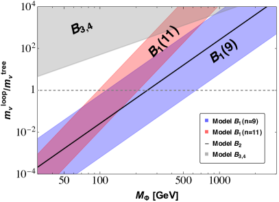
Figure 4: Ratio of the contribution to neutrino masses at one loop and at tree level versus the scalars mass in the limit $M_{\Psi}\gg M_{\Phi}$ for class-A (left) and class-B (right) models. The colored bands are obtained taking the couplings $\lambda_{i}\in[0.1;1]$. Notice that the dependence on $\lambda_{i}$ drops in models $\bf A_{1}$ and $\bf B_{2}$. For $\bf B_{3}$ and $\bf B_{4}$ the behaviour is very similar therefore we report only $\bf B_{3}$. See main text for further details.

In Fig. 4, we show how the ratio $m_{\nu}^{\rm loop}/m_{\nu}^{\rm tree}$ depends on the scalar masses, taking all the quartic couplings in the range [0.1, 1], considering Eqs. (29)-(34). It is interesting to notice how for the class-$\bf A$ models, the tree-level contribution may dominate considering the most favorable choice of the couplings if $M_{\Phi}<780$ GeV for $\bf A_{2}$ and $M_{\Phi}<500$ GeV for $\bf A_{1}$. In the class-$\bf B$ models the scalar masses for which the tree level can overcome the loop-level one are smaller in all the cases except for $\bf B_{1}$ ($n=9$), where we obtain $M_{\Phi}<640$ GeV. In particular, we have $M_{\Phi}<210\,,250$ GeV for $\bf B_{1}$ ($n=11$) and $\bf B_{2}$, respectively. For Models $\bf B_{3,4}$, the tree level contribution is always sub-leading because the scalar potential does not allow to induce small VEVs for $\Phi_{1}$ and $\Phi_{2}$ and the tree-level contribution is always proportional to either $v_{1}$ or $v_{2}$.

In the following, we analyse how the quartic couplings modify the ratio $m_{\nu}^{\text{loop}}/m_{\nu}^{\text{tree}}$ in the $\bf{A_{1}}$ and $\bf{B_{1}}$ models. Note that the couplings associated with lepton number violation (LNV) generate also a mass for pseudo-Nambu-Goldstone bosons, which should be larger than $m_{J}^{\rm min}=45$ GeV from $Z-$boson decays CMS:2022ett , see also Ref. us . In Model $\bf{A_{1}}$, there exists a single massive pseudo-Nambu-Goldstone boson, the pseudo-Majoron $J$; expanding its mass to first order in $\mathcal{O}(v_{1}/v)$, we obtain the lower limit

$$|\bar{\lambda}|\geq\dfrac{(m_{J}^{\mathrm{\rm min}})^{2}\,v_{1}}{3\,\sqrt{3}\,v^{3}}\;\,.$$ (35)

In Model $\bf{B_{1}}$, on the other hand, the presence of an explicitly broken additional $U(1)$ symmetry in the scalar potential allows for two massive pseudo-Nambu-Goldstone bosons ($J$ and $\Omega$). Therefore, we obtain the following lower limits

$$|\lambda_{1}|\geq\dfrac{2\,\sqrt{3}\,(m_{J}^{\mathrm{min}})^{2}\,v_{1}}{v^{3}}\;\,,$$ (36)

$$|\lambda_{2}|\geq\dfrac{2\,(m_{\Omega}^{\mathrm{min}})\,v_{2}}{v^{3}}\;\,.$$ (37)

Considering $v_{{1,2}}\simeq\mathcal{O}(1)$ GeV, these bounds read:

$$|\bar{\lambda}|\gtrsim 7\cdot 10^{-5}\quad\text{for $\bf{A_{1}}$}\,,$$ (38)

$$|\lambda_{1}|\gtrsim 10^{-3},\quad|\lambda_{2}|\gtrsim 8\cdot 10^{-4}\quad\text{for $\bf{B_{1}}$}\,.$$ (39)

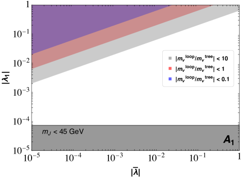
Figure 5: Contours of fixed $m_{\nu}^{\text{loop}}/m_{\nu}^{\text{tree}}$ in the plane of the LNV quartic couplings for Model ${\bf A_{1}}$. We also show the region excluded by the pseudo-Nambu-Goldstone mass.

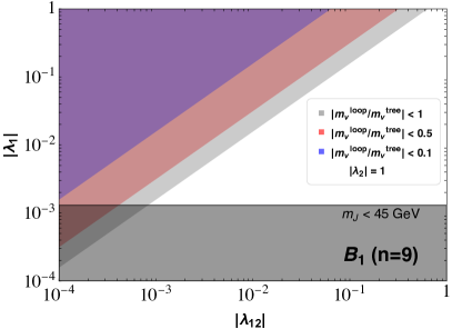
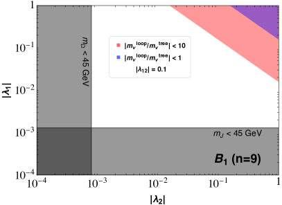
Figure 6: Same as Fig. 5 for Model ${\bf B_{1}}$, showing two different planes of the LNV quartic couplings.

In Figs. 5 and 6 we show, for Models ${\bf A_{1}}$ and ${\bf B_{1}}$, respectively, how the $\lambda$ couplings modify the $m_{\nu}^{\text{loop}}/m_{\nu}^{\text{tree}}$ ratio, reporting in shaded gray the excluded region due to the lower limits on pseudo-Nambu-Goldstone boson mass.

4 Dimension-$6$ Effective Operators

At low energies, integrating-out the heavy fermion mediators, dimension-$6$ Derivative operators are generated Herrero-Garcia:2016uab . Unlike the dimension-$5$ Weinberg-like operators, these do not violate lepton number, but may violate lepton flavor. In particular, after SSB they modify couplings to SM gauge bosons and they yield a non-unitary PMNS matrix, $U\equiv(1-\kappa)U_{L}$, once canonically normalised neutrino kinetic terms are constructed deGouvea:2015euy ; Blennow:2016jkn ; Malinsky:2009df ; Escrihuela:2016ube ; Akhmedov:1995ip ; Agarwalla:2021owd . In the standard seesaw scenarios such operators are discussed in Refs. Abada:2007ux ; Abada:2008ea . For instance, for seesaw Type-I, the dimension-6 operator generated reads

$$\mathcal{O}^{(0)}_{6}=\left(\overline{L}_{\alpha}\tilde{H}\right)i\not{\partial}\left(\tilde{H}^{\dagger}L_{\beta}\right)\,,$$ (40)

with $C^{(0)}_{6}=\left(y_{H}M_{N}^{-2}y_{H}^{\dagger}\right)_{\alpha\beta}$.

On general grounds, these dimension-$6$ operators are strongly suppressed because they have a similar structure as the dimension-$5$ ones responsible for neutrino masses and they are further suppressed by an additional power of the heavy mediator mass. Therefore, unless there exists a mechanism which decouples the dimension-$5$ and $6$ WCs allowing a low-scale seesaw, as discussed in Section 2.6, the associated phenomenological signatures are suppressed. As shown in Section 2.6.1, in the case Majorana mediators (Model $\bf A_{1}$), indeed an inverse seesaw scheme can be constructed. In this case, the larger Yukawas and smaller scales may yield significant contributions to dimension-$6$ operators. For the VL models (Models $\bf A_{2}$, $\bf B_{i}$), interestingly the product of Yukawas violates LN and enters in neutrino masses, as discussed in Section 2.6.2. Therefore, the contributions to some dimension-$6$ operators, which only depend individually on the either $y_{1}$ or $y_{2}$, can be significant.

In our genuine models, dimension-$6$ operators involving the new scalar multiplets will be generated at low energies. Namely, for models that have $\Phi_{1}$ and a fermion $\mathcal{F}$, we have

$$\mathcal{O}^{(1)}_{6}=\left(\overline{L}_{\alpha}{\Phi}_{1}\right)i\not{D}\left({\Phi}_{1}^{\dagger}L_{\beta}\right)\,,$$ (41)

with $C^{(1)}_{6}=\left(y_{1}M_{\mathcal{F}}^{-2}y_{1}^{\dagger}\right)_{\alpha\beta}$. Here

$$\not{D}=\not{\partial}-i\;\dfrac{g}{2}\Gamma^{i}\not{W}^{i}-i\;\dfrac{g^{\prime}}{2}Y\not{B}\$$ (42)

is the covariant derivative, where $\Gamma^{i}$ are the SU(2) generators of the representation of hypercharge $Y$ on which it acts, and the identity matrix is implicit in the hypercharge term. Similarly, for $\bf B_{i}$-models that also have a second multiplet, $\Phi_{2}$, identical operators $\mathcal{O}^{(2)}_{6}$ are generated, with the substitution $y_{1}\rightarrow y_{2}$ in $C^{(1)}_{6}\rightarrow C^{(2)}_{6}$. In principle, irrespective of neutrino masses and LNV, given the small VEVs, these will be further suppressed compared to $\mathcal{O}^{(0)}_{6}$. Therefore, also the modifications to the gauge boson couplings are expected to be generically smaller than in Type-I inverse seesaw.

For the $\bf A_{1}$ model, $\mathcal{O}^{(1)}_{6}$ as in Eq. (41) is generated with $C^{(1)}_{6}=(y_{1}M_{\Sigma}^{-2}y_{1}^{\dagger})_{\alpha\beta}$. For the $\bf A_{2}$ model, both $\mathcal{O}^{(0)}_{6}$ with just the SM Higgs can be built, as in Eq. (40), with coupling $C^{(0)}_{6}=(y_{H}M_{\mathcal{F}}^{-2}y_{H}^{\dagger})_{\alpha\beta}$ Herrero-Garcia:2016uab , and also $\mathcal{O}^{(1)}_{6}$ with the new multiplet $\Phi_{1}$ with $C^{(1)}_{6}=(y_{1}M_{\mathcal{F}}^{-2}y_{1}^{\dagger})_{\alpha\beta}$, as in Eq. (41). Unless there are large hierarchies in the Yukawas, the former one is expected to dominate. However, given that neutrino masses can be reproduced by taking a hierarchy of Yukawas and VEVs, for instance $y_{1}v_{1}\ll y_{H}v_{H}$, there may be significant effects from $C^{(0)}_{6}$, with $C^{(1)}_{6}\ll C^{(0)}_{6}$. As discussed in Section 2.6.2, these hierarchical vector-like versions are the equivalent of inverse seesaw of hypercharge-less fermions. The key point is that the product of Yukawas and VEVs violates lepton number, while each of them individually does not and may contribute to $n=6$ operators.

Regarding the $\bf B_{i}$ models, where we add two different scalar multiplets with a vector-like mediator of mass $M_{\mathcal{F}}$, the integration of the heavy fields leads to both $\mathcal{O}^{(1)}_{6}$ and $\mathcal{O}^{(2)}_{6}$, with $C^{(1)}_{6}=\left(y_{1}M_{\mathcal{F}}^{-2}y_{1}^{\dagger}\right)_{\alpha\beta}$ and $C^{(2)}_{6}=\left(y_{2}M_{\mathcal{F}}^{-2}y_{2}^{\dagger}\right)_{\alpha\beta}$, respectively. Similarly to the case of the $\bf A_{2}$ model, neutrino masses can be reproduced by taking a hierarchy of Yukawas and VEVs, for instance $y_{1}v_{1}\ll y_{2}v_{2}$. Then, $C^{(2)}_{6}$ may be large, with $C^{(1)}_{6}\ll C^{(2)}_{6}$. Again, these are the equivalent of the inverse seesaw version of Model $\bf A_{1}$. It is interesting to mention that dimension$-6$ operators may still be generated in $\mathbf{B_{i}}$ models if only one of the two new scalar multiplets take a VEV, differently from the neutrino masses case for which both non-zero VEVs are required.

	$\mathcal{O}^{(0)}_{6}$			$\mathcal{O}^{(1)}_{6}$
Model	$Z\;\nu_{\alpha}\nu_{\beta}$	$Z\;e_{\alpha}e_{\beta}$	$W\;e\nu$	$Z\;\nu_{\alpha}\nu_{\beta}$	$Z\;e_{\alpha}e_{\beta}$	$W\;e\nu$
$\bf A_{1}$	$-$✘	$-$✘	$-$✘	$\dfrac{1}{2}$	$-$$-\dfrac{3}{4}$	$-$$\dfrac{17}{4}$
$\bf A_{2}$	$-$$1$	$-\dfrac{1}{2}$	$-$$\dfrac{1}{2}$	$-\dfrac{\sqrt{3}}{2}$	$-$$0$	$-\dfrac{\sqrt{3}}{6}$

Table 4: Corrections to the $Z$- and $W$-boson couplings for the $\bf A_{i}$ models. For Model $\bf A_{2}$, the $\mathcal{O}^{(1)}_{6}$ contribution is sub-leading with respect to the $\mathcal{O}^{(0)}_{6}$ one for $y_{1}v_{1}\ll y_{H}v$. The $Z$-boson couplings are in units of $\kappa_{\alpha\beta}e/(2c_{W}\;s_{W})$, while $W$-boson couplings are in units of $\kappa_{\alpha\beta}e/(2\sqrt{2}s_{W})$. For instance, for Model $\bf A_{2}$, the value of $\kappa$ for $\mathcal{O}^{(0)}_{6}$ is $\kappa^{(0)}=\left(y_{H}M_{\mathcal{F}}^{-2}y_{H}^{\dagger}\right)v^{2}$ and for $\mathcal{O}^{(1)}_{6}$ is $\kappa^{(1)}=\left(y_{1}M_{\mathcal{F}}^{-2}y_{1}^{\dagger}\right)v^{2}_{1}$. Notice the different values to Ref. Herrero-Garcia:2016uab for $\bf A_{2}$, due to the different normalization that we used for $\left\langle H\right\rangle$.

	$\mathcal{O}^{(1)}_{6}$			$\mathcal{O}^{(2)}_{6}$
Model	$Z\;\nu_{\alpha}\nu_{\beta}$	$Z\;e_{\alpha}e_{\beta}$	$W\;e\nu$	$Z\;\nu_{\alpha}\nu_{\beta}$	$Z\;e_{\alpha}e_{\beta}$	$W\;e\nu$
$\bf B_{1}$	$-\dfrac{3}{4}$	$-$$\dfrac{1}{2}$	$-$$\dfrac{17}{4}$	$-$$\dfrac{3}{4}$	$-3$	$-\dfrac{3}{4}$
$\bf B_{2}$	$-$$0$	$-$$0$	$-$$4$	$-$$\dfrac{3}{4}$	$-\dfrac{1}{4}$	$-\dfrac{1}{4}$
$\bf B_{3}$	$-2$	$-$$0$	$-\dfrac{1}{2}$	$-1$	$-$$\dfrac{3}{4}$	$-\dfrac{5}{8}$
$\bf B_{4}$	$-$$\dfrac{3}{4}$	$-\dfrac{1}{4}$	$-\dfrac{1}{4}$	$-$$0$	$-$$0$	$-$$\dfrac{1}{2}$

Table 5: Same as Table 4 for the $\bf B_{i}$ models. The $\mathcal{O}_{6}^{(2)}$ contribution will dominate w.r.t. that of $\mathcal{O}_{6}^{(1)}$ for $y_{2}v_{2}\gg y_{1}v$

When the scalars take VEVs, these operators modify the kinetic terms of the lepton doublets. Therefore, in order to obtain canonically normalized kinetic terms, we need to rescale the components lepton doublet fields ($L\equiv(\nu,l)$): $\nu\rightarrow(1+\zeta_{\nu}\,\kappa)^{-1/2}\,\nu$ and $l\rightarrow(1+\zeta_{l}\,\kappa)^{-1/2}\,l$, where $\zeta_{\nu,l}$ are numerical factors (reported in Appendix B) and $\kappa$ is a small parameter proportional to the dimension-$6$ couplings times the VEVs. For instance, for $\mathcal{O}^{(1)}_{6}$ with lepton flavors $\alpha\beta$, the $\kappa$ coupling is given by

$$\kappa^{(1)}_{\alpha\beta}=(C^{(1)}_{6})_{\alpha\beta}\,v_{1}^{2}\,.$$ (43)

After an expansion in $\kappa$, we get modified couplings of the gauge bosons to the SM leptons. In Tables 4 and 5 we present the modifications to SM couplings for Models $\bf A_{i}$ and $\bf B_{i}$, respectively. The corrections of $Z$-boson couplings to flavors $\alpha\beta$ are proportional to $\kappa_{\alpha\beta}e/(2s_{W}c_{W})$, while the $W$-boson couplings are proportional to $\kappa_{\alpha\beta}e/(2\sqrt{2}s_{W})$. Note that $Z$-boson couplings are in all cases with left-handed lepton doublets.

5 Phenomenology

In this section we study the phenomenological signatures generated in the various models.

5.1 Universality violation and non-unitarity of the leptonic mixing matrix

The dimension-$6$ operators modify the couplings of leptons to SM gauge bosons after SSB. In particular, they yield a non-unitary PMNS matrix, as well as $Z$-boson FCNC. For Model ${\bf A_{2}}$, also Higgs lepton flavor violating couplings are generated, see Ref. Herrero-Garcia:2016uab for details. The modified couplings due to $\mathcal{O}^{(0,1)}_{6}$ are given in Table 4 for the $\bf A_{i}$ models, and those due to $\mathcal{O}^{(1,2)}_{6}$ are provided in Table 5 for the $\bf B_{i}$ models. In the case of low-scale seesaws, these may give observable signals, as discussed in Section 2.6.

The most constraining limits on the dimension-$6$ operators come from radiative LFV processes, $Z$-mediated tree-level LFV, non-universal decays, and from the non-unitarity of the PMNS mixing matrix. Although flavor-dependent, the typical constraints read

$$\kappa^{(1)}_{\alpha\beta}\equiv c^{(1)}_{\alpha\beta}v^{2}_{1}=\left(y_{1}M_{F}^{-2}y_{1}^{\dagger}\right)_{\alpha\beta}v_{1}^{2}\lesssim\mathcal{O}(10^{-3})\,.$$ (44)

In Table 6 we provide the limits on the diagonal (off-diagonal) entries of the $\kappa$ matrices of the different models for different flavors, from non-universal (LFV) $Z$-decays. The relevant expressions for the processes can be found in Section 3.2 of Ref. Herrero-Garcia:2016uab . As the matrix is Hermitian and positive-definite, the off-diagonal couplings are bounded by the diagonal ones, $|\kappa_{\ell\ell^{\prime}}|<\sqrt{\kappa_{\ell\ell}\kappa_{\ell^{\prime}\ell^{\prime}}}$.

		Upper limits
Model	$\mathcal{O}_{6}^{(i)}$	$\kappa_{ee}$	$\kappa_{\mu\mu}$	$\kappa_{\tau\tau}$	$\kappa_{\tau\mu}$	$\kappa_{\tau e}$	$\kappa_{\mu e}$
$\bf A_{1}$	$\mathcal{O}_{6}^{(1)}$	$<0.0013$	$<0.0028$	$<0.0053$	$<0.0005$	$<0.0005$	$<1.3\times 10^{-6}$
$\bf A_{2}$	$\mathcal{O}_{6}^{(0)}$	$<0.0019$	$<0.0042$	$<0.0079$	$<0.0007$	$<0.0008$	$<2\times 10^{-6}$
$\bf B_{1}$	$\mathcal{O}_{6}^{(1)}$	$<0.0036$	$<0.0042$	$<0.0012$	$<0.0007$	$<0.0008$	$<2\times 10^{-6}$
$\bf B_{1}$	$\mathcal{O}_{6}^{(2)}$	$<0.0003$	$<0.0007$	$<0.0013$	$<0.0001$	$<0.0001$	$<3.3\times 10^{-7}$
$\bf B_{2}$	$\mathcal{O}_{6}^{(2)}$	$<0.0038$	$<0.0084$	$<0.0159$	$<0.0014$	$<0.0016$	$<4\times 10^{-6}$
$\bf B_{3}$	$\mathcal{O}_{6}^{(2)}$	$<0.0024$	$<0.0028$	$<0.0008$	$<0.0005$	$<0.0005$	$<1.3\times 10^{-6}$
$\bf B_{4}$	$\mathcal{O}_{6}^{(1)}$	$<0.0038$	$<0.0084$	$<0.0159$	$<0.0014$	$<0.0016$	$<4\times 10^{-6}$

Table 6: Limits on the dimension-6 operators from $Z$-boson mediated tree-level non-universal and LFV decays. For all models but ${\bf B_{1}}$, only one operator has a non-zero correction to $Ze_{\alpha}e_{\beta}$ and the corresponding limits are quoted. For ${\bf B_{1}}$, we derive the limits assuming only of them contributes while neglecting the other one.

5.2 Lepton Flavor Violation

The new seesaw models generate LFV decays, which are absent in the SM. The experimental limits on these observables set bounds on the Yukawa couplings of the new scalars with charged leptons and the masses of the new particles. We focus on some of the most constraining processes, which are the radiative decays $l_{\alpha}\rightarrow l_{\beta}\gamma$. In our models, the analytical expression for ${\rm BR}(l_{\alpha}\rightarrow l_{\beta}\gamma)$ may be written as

$${\rm BR}(l_{\alpha}\rightarrow l_{\beta}\gamma)= \frac{3\alpha_{\rm em}}{64\pi G_{F}^{2}}\,\bigg{|}\sum_{k=1}^{N_{\Phi}}\sum_{l=1}^{N_{\Psi}}y_{k}^{l{\beta^{\ast}}}y_{k}^{l\alpha}\sum_{j=1}^{n_{\Phi}}\sum_{i=1}^{n_{\psi}}\frac{c^{2}_{Q_{\Psi_{i}}Q_{\Phi_{j}}}}{M_{\Phi_{j}}^{2}}\left[Q_{\psi_{i}}f_{\psi}(r)+Q_{\Phi_{j}}f_{\Phi}(r)\right]\bigg{|}^{2}$$

$$\times{\rm BR}(l_{\alpha}\rightarrow l_{\beta}\nu_{\alpha}\bar{\nu_{b}})\,,$$ (45)

where $r\equiv M_{\psi_{i}}^{2}/M_{\Phi_{j}}^{2}$, $\alpha_{\rm em}=e^{2}/(4\pi)$ is the fine structure constant and $G_{F}$ is Fermi’s decay constant. Experimentally, the branching ratio ${\rm BR}(l_{\alpha}\rightarrow l_{\beta}\nu_{\alpha}\bar{\nu_{b}})$ is equal to $\{1,0.178,0.174\}$ for $\alpha\beta=\{\mu e,\tau e,\tau\mu\}$, respectively ParticleDataGroup:2022pth . $N_{\Phi(\Psi)}$ denotes the number of new scalars (fermionic mediators, $\Psi=\Sigma,\mathcal{F}$) in the model, whereas $n_{\Phi}$ and $n_{\psi}$ denote the number of components in the scalar and fermion multiplets, respectively. $Q$ denotes the charges of the scalar and fermion components in the loop such that $Q_{l_{\alpha}}=Q_{\psi_{i}}-Q_{\Phi_{j}}$, and $c_{Q_{\psi_{i}}Q_{\Phi_{j}}}$ is the numerical coefficient of the term containing a scalar (fermion) component with charge $Q_{\Phi_{j}}$ ($Q_{\psi_{i}}$) in the expansion of the Yukawa Lagrangian in tensor notation. Finally, the loop functions are given by Lavoura:2003xp

$$f_{\psi}(x) =\frac{2+3x-6x^{2}+x^{3}+6x\ln{x}}{6(1-x)^{4}}\approx\frac{1}{6x}({\rm for~{}}x\gg 1)\,,$$

$$f_{\Phi}(x) =\frac{1-6x+3x^{2}+2x^{3}-6x^{2}\ln{x}}{6(1-x)^{4}}\approx\frac{1}{3x}({\rm for~{}}x\gg 1)\,,$$

where in the last step we approximated them for large $x$. We make the following assumptions for Eq. (5.2) to simplify the resulting expression:

• The components within the multiplets are degenerate i.e., $M_{\Phi_{j}}=M_{\Phi}\,,M_{\psi_{i}}=M_{\Psi}$,

• Whenever there are two or more new scalars or fermions in the model, we take their masses to be the same i.e, $M_{\Phi_{1}}=M_{\Phi_{2}}=M_{\Phi}$,

• We ignore the mixing among the scalars, and among SM and heavy fermions,

• We consider only the contributions coming from BSM states in the loop. Further, in the limit $M_{\Sigma,\mathcal{F}}\gg M_{\Phi}$, the dependence on scalar masses is negligible and the bounds can be expressed solely in terms of the fermion mediator mass only.

The most stringent bound comes from radiative muon decays, ${\rm BR}(\mu\rightarrow e\gamma)<4.2\times 10^{-13}$ at 90% CL MEG:2016leq , which is much stronger than the radiative $\tau$-lepton decays, ${\rm BR}(\tau\rightarrow e\gamma)<3.3\times 10^{-8}$ and ${\rm BR}(\tau\rightarrow\mu\gamma)<4.4\times 10^{-8}$ at 90% CL BaBar:2009hkt .

To illustrate the limits, let us consider the model $\bf A_{1}$ which contains one new scalar multiplet $\mathbf{4}_{-1/2}^{S}$ and one fermionic quintuplet $\mathbf{5}_{0}^{F}$. Given the charged lepton Yukawa Lagrangian expansion

$$y_{1}\bar{L}\Phi\Sigma=y_{1}\bar{l}\left(\Sigma^{--}\Phi^{+}-\frac{\sqrt{3}}{2}\Sigma^{-}\Phi^{0}+\frac{1}{\sqrt{2}}\Sigma^{0}\Phi^{-}-\frac{1}{2}\Sigma^{+}\Phi^{--}\right)\,,$$ (46)

we can write the branching ratio for $\mu\rightarrow e\gamma$ as

$${\rm BR}(\mu\rightarrow e\gamma)=\frac{3\alpha_{\rm em}}{64\pi G_{F}^{2}}\left|\frac{y_{1}^{{e^{\ast}}}y_{1}^{\mu}}{M_{\Phi}^{2}}\,Z_{\Phi}^{\rm A1}\left(\frac{M_{\Sigma}^{2}}{M_{\Phi}^{2}}\right)\right|^{2}\,,$$ (47)

with

$$Z_{\Phi_{1}}^{\bf A_{1}}(x) =\frac{1}{2}f_{\Phi}(x)-\frac{3}{4}f_{\psi}(x)-\left[2f_{\psi}(x)+f_{\Phi}(x)\right]+\frac{1}{4}\left[f_{\psi}(x)+2f_{\Phi}(x)\right]\,.$$ (48)

Imposing the current experimental upper bound on ${\rm BR}(\mu\rightarrow e\gamma)$, we get

$$\frac{|y_{1}^{{e^{\ast}}}y_{1}^{\mu}|}{({M_{\Sigma}}/{\rm TeV})^{2}}\lesssim 2\times 10^{-4}\,.$$ (49)

Similarly, bounds on various Yukawa combinations from other LFV decays can be calculated.

		Upper limits
Model	Yukawa combination	$\alpha\beta=\mu e$	$\alpha\beta=\tau e$	$\alpha\beta=\tau\mu$
$\bf A_{1}$	$|y_{1}^{{\beta^{\ast}}}y_{1}^{\alpha}|({\rm TeV}/{M_{\Sigma}})^{2}$	$<0.0002$	$<0.13$	$<0.16$
$\bf A_{2}$	$|y_{1}^{{\beta^{\ast}}}y_{1}^{\alpha}|({\rm TeV}/{M_{\mathcal{F}}})^{2}$	$<0.0004$	$<0.24$	$<0.28$
$\bf B_{1}$	$|y_{1}^{{\beta^{\ast}}}y_{1}^{\alpha}-0.5\,y_{2}^{{\beta^{\ast}}}y_{2}^{\alpha}|({\rm TeV}/{M_{\mathcal{F}}})^{2}$	$<0.0004$	$<0.29$	$<0.34$
$\bf B_{2}$	$|y_{1}^{{\beta^{\ast}}}y_{1}^{\alpha}-50\,y_{2}^{{\beta^{\ast}}}y_{2}^{\alpha}|({\rm TeV}/{M_{\mathcal{F}}})^{2}$	$<0.0011$	$<0.72$	$<0.84$
$\bf B_{3}$	$|y_{1}^{{\beta^{\ast}}}y_{1}^{\alpha}-2.12\,y_{2}^{{\beta^{\ast}}}y_{2}^{\alpha}|({\rm TeV}/{M_{\mathcal{F}}})^{2}$	$<0.0002$	$<0.15$	$<0.18$
$\bf B_{4}$	$|y_{1}^{{\beta^{\ast}}}y_{1}^{\alpha}+6.6\,y_{2}^{{\beta^{\ast}}}y_{2}^{\alpha}|({\rm TeV}/{M_{\mathcal{F}}})^{2}$	$<0.0004$	$<0.24$	$<0.28$

Table 7: $90\%$CL limits on combination of Yukawa couplings and fermion masses from lepton-flavor-violating radiative decays for the different models.

In models of Type-${\bf B}$, which contain two new scalars, both Yukawas $y_{1}$ and $y_{2}$ in Eq. (9) enter in the decay. Note that the Yukawa combination that is constrained from LFV decays is different from the one entering in the expression of neutrino masses, where the product of both couplings enters. For example, consider the model $\bf B_{1}$ which contains the scalar multiplets $\mathbf{4}_{1/2}^{S}$, $\mathbf{4}_{-3/2}^{S}$ and a vector-like mediator $\mathbf{5}_{0}^{F}$. The relevant charged lepton Yukawa Lagrangian is

$$\bar{L}\Phi_{1}\mathcal{F}_{R} =\bar{l}\left(\mathcal{F}_{R}^{---}\Phi_{1}^{++}-\frac{\sqrt{3}}{2}\mathcal{F}_{R}^{--}\Phi_{1}^{+}-\frac{1}{\sqrt{2}}\mathcal{F}_{R}^{-}\Phi_{1}^{0}-\frac{1}{2}\mathcal{F}_{R}^{0}\Phi_{1}^{-}\right)\,,$$

$$\bar{L}\Phi_{2}\mathcal{F}_{L}^{c} =\bar{l}\left(-{\mathcal{F}_{L}^{+}}^{c}\Phi_{2}^{0}-\frac{\sqrt{3}}{2}{\mathcal{F}_{L}^{0}}^{c}\Phi_{2}^{-}-\frac{1}{\sqrt{2}}{\mathcal{F}_{L}^{-}}^{c}\Phi_{2}^{--}-\frac{1}{2}{\mathcal{F}_{L}^{--}}^{c}\Phi_{2}^{---}\right)\,,$$ (50)

which gives

$${\rm BR}(l_{\alpha}\rightarrow l_{\beta}\gamma)=\frac{3\alpha_{\rm em}}{64\pi G_{F}^{2}}\,\bigg{|}\frac{y_{1}^{\beta\ast}y_{1}^{\alpha}}{M_{\Phi_{1}}^{2}}Z_{\Phi_{1}}^{\rm B1}\left(\frac{M_{\mathcal{F}}^{2}}{M_{\Phi_{1}}^{2}}\right)+\frac{y_{2}^{\beta\ast}y_{2}^{\alpha}}{M_{\Phi_{2}}^{2}}Z_{\Phi_{2}}^{\rm B1}\left(\frac{M_{\mathcal{F}}^{2}}{M_{\Phi_{2}}^{2}}\right)\bigg{|}^{2}\times{\rm BR}(l_{\alpha}\rightarrow l_{\beta}\nu_{\alpha}\bar{\nu_{b}})\,,$$ (51)

with

$$Z_{\Phi_{1}}^{\bf B_{1}}(x) =\left\{-[3f_{\psi}(x)+2f_{\Phi}(x)]-\frac{3}{4}[2f_{\psi}(x)+f_{\Phi}(x)]-\frac{1}{2}[f_{\psi}(x)]+\frac{1}{4}[f_{\Phi}(x)]\right\}\,,$$

$$Z_{\Phi_{2}}^{\bf B_{1}}(x) =\left\{-[f_{\psi}(x)]+\frac{3}{4}[f_{\Phi}(x)]+\frac{1}{2}[f_{\psi}(x)+2f_{\Phi}(x)]+\frac{1}{4}[2f_{\psi}(x)+3f_{\Phi}(x)]\right\}\,.$$ (52)

Taking $x\gg 1$, we can simplify the above expressions as $Z_{\Phi_{1}}^{\rm B1}(x)\approx-5/(6x)$ and $Z_{\Phi_{2}}^{\rm B1}(x)\approx 5/(12x)$. Then, the bound from BR$(\mu\rightarrow e\gamma)$ reads

$$\frac{|y_{1}^{e\ast}y_{1}^{\mu}-0.5\,y_{2}^{e\ast}y_{2}^{\mu}|}{(M_{\mathcal{F}}/{\rm TeV})^{2}}<4.3\times 10^{-4}\,.$$ (53)

The bounds on the Yukawa combinations from LFV decays for all models are summarised in Table 7. Let us also mention that the Yukawa structure can be determined in terms of neutrino parameters using the Casas-Ibarra parameterization for Majorana-like mediators Casas:2001sr (Model ${\bf A_{1}}$), whereas for vector-like mediators in ${\bf B}$-type models, the approach used in the Generalized Scotogenic Model can be followed Hagedorn:2018spx . This would be useful to do a parameter scan of the models, which is beyond the scope of this work.

Moreover, one can also study other LFV processes such as $l_{\alpha}\rightarrow 3l_{\beta}$ and $\mu-e$ conversion in nuclei in our models Ren:2011mh ; Toma:2013zsa ; Felkl:2021qdn . The experimental sensitivities for these processes are expected to improve by four orders of magnitude in the coming years Perrevoort:2023jry and it would be worth studying them in detail for a specific model. The former process can receive contributions from penguins and box-type diagrams, however, for small values of Yukawas (as seen in the analysis above), the box-type contribution will be subdominant, and using dipole dominance approximation, we can write Hagedorn:2018spx

$${\rm BR}(\mu\rightarrow 3e) \approx\frac{\alpha_{\rm em}}{8\pi}\left(\frac{16}{3}\ln\frac{m_{\mu}}{m_{e}}-\frac{22}{3}\right)\times{\rm BR}(\mu\rightarrow e\gamma)$$

$$\approx 0.006\times{\rm BR}(\mu\rightarrow e\gamma)\,.$$ (54)

The above approximation can be used to further constrain the Yukawas, when new data becomes available in the future.

Finally, there also exist implications for charged lepton electric dipole moments (EDM) in our models, which are generated at the two-loop level. The electric dipole moments for the minimal scotogenic model Ma:2006km were calculated in Ref. Abada:2018zra . The sensitivity to the muon EDM is expected to improve by more than three orders of magnitude at the muEDM experiment based in PSI Schmidt-Wellenburg:2023aga . It is possible to construct scotogenic-like models from our models as well, as we discuss below.

6 (Generalised) Scotogenic-like models

Models where neutrino masses arise purely at the loop level are interesting because a viable dark matter (DM) candidate may be easily embedded, see Ref. Restrepo:2013aga ; Cai:2017jrq . Indeed, if the new scalar and Majorana (vector-like) fermion multiplets transform under a $Z_{2}$ ($U(1)$) dark symmetry, the lightest of them, if neutral, may be a viable DM candidate. If the particle has $Y=0$, it may be allowed by direct detection (DD) constraints if the Higgs portal couplings in the potential are small enough. For the $Y\neq 0$ scenarios, DD excludes them, unless the DM candidate is a CP-even (odd) scalar with a sufficiently-large mass splitting (i.e., $\Delta m_{\Phi}\gtrsim\mathcal{O}\,(\text{MeV})$) with its CP-odd (even) counterpart Cirelli:2005uq ; Hambye:2009pw . Another way to have viable scalar DM candidate from a multiplet with $Y\neq 0$ is to mix the neutral component with a real scalar singlet, as in the ScotoSinglet Model Beniwal:2020hjc . These (generalised) Scotogenic-like models are:

• Scotogenic-like Model $\bf A^{\prime}_{1}$: with a $Z_{2}$ symmetry, such that $\Phi\rightarrow-\Phi$ and $\Sigma\rightarrow-\Sigma$. Imposing the $Z_{2}$ symmetry kills the terms involving only a single scalar multiplet in the scalar potential.

• Generalised Scotogenic-like Model $\bf B^{\prime}_{i}$: with a new global $U(1)$ symmetry, such that only $\Phi_{1}$, $\Phi_{2}$ and $\mathcal{F}$ transform non-trivially, for example: $q_{\Phi_{1}}=1,q_{\Phi_{2}}=-1$ and $q_{\mathcal{F}}=-1$, the generalised scotogenic equivalent term will be $HH\Phi_{1}\Phi_{2}$. Note that the same term can lead to the needed mass splitting among the real and imaginary parts of the scalar multiplets with $Y\neq 0$. It can be seen that this new global symmetry can be identified as the $U(1)_{X}$ accidental symmetry of the scalar potential involving two new scalar multiplets, see Table 3 of Ref. us .

Note that as Model $\bf A_{2}$ is the only model that includes the SM Higgs to generate neutrino masses radiatively via the term $HHH\Phi^{\ast}$, neither $Z_{2}$ nor $U(1)$ symmetry can be imposed to accommodate a DM candidate.

Model	New Fields	Sym.	DM candidates	DM Mass (TeV)
$\bf A^{\prime}_{1}$	$\Phi_{1}=4_{-1/2}^{S}\,,\Sigma=5_{0}^{F}$	$Z_{2}$	$4_{-1/2}^{S}$, $5_{0}^{F}$	$M_{\Phi_{1}}\approx 3.2,M_{\Sigma}\approx 10$
$\bf A^{\prime}_{2}$	$\Phi_{1}=4_{-3/2}^{S}\,,\mathcal{F}=3_{-1}^{F}$	$-$	$-$	$-$
$\bf B^{\prime}_{1}$	$\Phi_{1}=4_{1/2}^{S}\,,\Phi_{2}=4_{-3/2}^{S}\,,\mathcal{F}=5_{-1}^{F}$	$U(1)$	$4_{1/2}^{S}\,,4_{-3/2}^{S}$	$M_{\Phi_{1}}\approx 3.2,M_{\Phi_{2}}\approx 3.5$
$\bf B^{\prime}_{2}$	$\Phi_{1}=3_{0}^{S}\,,\Phi_{2}=5_{-1}^{S}\,,\mathcal{F}=4_{-1/2}^{F}$	$U(1)$	$3_{0}^{S}\,,5_{-1}^{S}$	$M_{\Phi_{1}}\approx 2.5,M_{\Phi_{2}}\approx 3.4$
$\bf B^{\prime}_{3}$	$\Phi_{1}=5_{-2}^{S}\,,\Phi_{2}=5_{1}^{S}\,,\mathcal{F}=4_{3/2}^{F}$	$U(1)$	$5_{-2}^{S}\,,5_{1}^{S}$	$M_{\Phi_{1}}\approx 3.9,M_{\Phi_{2}}\approx 3.4$
$\bf B^{\prime}_{4}$	$\Phi_{1}=5_{-1}^{S}\,,\Phi_{2}=5_{0}^{S}\,,\mathcal{F}=4_{1/2}^{F}$	$U(1)$	$5_{-1}^{S}\,,5_{0}^{S}$	$M_{\Phi_{1}}\approx 3.4,M_{\Phi_{2}}\approx 9.4$

Table 8: List of (Generalised) Scotogenic-like models which generate neutrino masses at one loop. We give the stabilising symmetry in the third column and the possible DM candidates in the fourth column. The mass for the DM candidate that reproduces the observed relic abundance is listed in the last column, including non-perturbative effects for the $Y=0$ candidates Cirelli:2007xd .

In Table 8 we summarise the Scotogenic-like models, labeled by $\bf A_{i}^{\prime}$ and $\bf B_{i}^{\prime}$ outlining their dark symmetry and their potentially-viable DM candidates. We also indicate the corresponding DM mass required to reproduce the DM relic abundance, $\Omega_{\rm DM}h^{2}=0.12\pm 0.0012$ where we assume that the neutral component of only one of the candidates makes up the total relic abundance. We have computed the masses following the approach of Ref. Cirelli:2007xd , where all co-annihilations (both $s$-wave and $p$-wave) of the DM component along with the relevant RGE corrections have been taken into account in the perturbative approximation. Furthermore, for candidates with $Y=0$, the non-perturbative Sommerfeld correction becomes quite important, especially for multiplets belong to higher $SU(2)$ representation, which enhances the annihilation cross-section compared to the perturbative approach, thus leading to larger DM masses in order to obtain the correct relic abundance. Therefore, the masses indicated for $3_{0}^{S},5_{0}^{S}$ and $5_{0}^{F}$ are obtained after including these non-perturbative effects Cirelli:2007xd . The precise computation of the DM masses corresponding to each multiplet after taking all these effects into account and a detailed analysis of direct and indirect detection limits would be interesting, but it is quite involved and beyond the scope of the present work.

7 Conclusions

The three standard seesaw mechanisms explaining small neutrino masses involve the SM Higgs doublet. In presence of new scalar and fermion multiplets, several other options emerge. One of the main advantages of these higher-representation seesaw models is that the vacuum expectation values (VEVs) of the new scalars, and consequently neutrino masses, are suppressed for reasons unrelated to the violation of lepton number: namely, the constraints stemming from the $\rho$ parameter due to the violation of custodial symmetry  us .

In this work, we have studied possible seesaw scenarios that do not involve the states present in the standard seesaws — neither the same fermions nor contributions that solely depend on the SM Higgs doublet VEV. These requirements narrow down the options to $2,(4)$ models featuring $1,(2)$ new scalar multiplet(s) up to quintuplet SU(2) representations. Only one involves a Majorana fermion mediator, while the rest involve vector-like mediators. These models are interesting due to their richer phenomenology compared to the standard Type-I seesaw scenario. In Ref. us we have studied the scalar phenomenology, while here we focus on the fermion phenomenology.

Furthermore, low-energy versions can be constructed in all cases, with some small parameter controlling the violation of lepton number, such as the Majorana mass $\mu_{L}$ in the inverse seesaw variant of Model ${\bf A_{1}}$ (see Eq. (22)), or a Yukawa coupling for the other models featuring vector-like fermions, for instance, $y_{1}$ in Eq. (27). In these low-energy versions, the effects of dimension-$6$ operators may be significant. In fact, the latter may generate substantial contributions to lepton flavor-violating observables, as well as to the non-unitarity of the PMNS mixing matrix and non-universal decays of the $Z$-boson.

In the considered seesaw models, one-loop corrections to neutrino masses are also present. Specifically, in Models ${\bf B_{3,4}}$, when TeV-scale scalars and order one couplings are involved, these loop contributions dominate. Additionally, it is interesting to note that, in certain instances, (Generalized) Scotogenic-like models capable of generating neutrino masses solely at one loop can be formulated. For scenarios where the fermion is Majorana (vector-like), a new $Z_{2}$ (global U(1)) symmetry must be imposed. In some of the resulting scenarios, a potentially viable DM candidate naturally emerges.

Let us briefly consider the possibility of leptogenesis in these scenarios. As the scalar multiplets acquire smaller VEVs, one might expect the lower bound on the mediator mass to roughly scale by the ratio of $v_{i}/v$ compared to the lower bound of $\mathcal{O}(10^{9})$ GeV for fermion singlets Davidson:2002qv . However, these new multiplets possess gauge interactions that deplete their population in the early universe, consequently suppressing the efficiency for leptogenesis. For instance, in the case of fermion triplets, the required mass of the lightest fermion triplet is estimated to be around $\mathcal{O}(10^{10})$ GeV Hambye:2012fh , assuming a hierarchical spectrum of the added fermion mediators to the model. In a related study Vatsyayan:2022rth , it was demonstrated that even if the fermion triplet couples to a new scalar doublet obtaining a VEV significantly lower than the SM Higgs, the scale can only be lowered to $10^{6}$ GeV (including flavor effects). Consequently, we anticipate that for multiplets belonging to higher $SU(2)$ representations, the constraints become more stringent due to their multiply-charged states and stronger gauge interactions. This suggests a necessity for heavy fermion masses of approximately $\mathcal{O}(10^{10})$ GeV or higher for successful leptogenesis in such scenarios. Therefore, accommodating low-scale leptogenesis within these models appears to be challenging.

In conclusion, while somewhat less minimal compared to standard seesaws, the models analysed in this study are intriguing and offer a rich phenomenology, particularly in their low-energy versions. Should large SU(2) representations be discovered, this research could offer valuable insights into their impact on the generation of light neutrino masses.

Appendix A Naturalness considerations

Since the new scalars take VEVs, their masses are bounded from above, i.e., they should be below the TeV scale. On the other hand, being scalars, there is the well-known hierarchy problem due to the presence of heavy scales, in this case, the heavy fermion masses $m_{\Psi}$. In seesaw Type-I, the one-loop correction to the Higgs boson self-energy from light and heavy sterile neutrinos ($N_{R}$) in the loop reads

$$\delta_{\rm\overline{MS}}\,m^{2}_{h}=\frac{m_{\nu}m_{N_{R}}^{3}}{4\pi v^{2}}\left[\log\left(\frac{m^{2}_{N_{R}}}{\mu^{2}}-1\right)\right]\,,$$ (55)

in the $\overline{\rm MS}$ scheme Vissani:1997ys ; Farina:2013mla ; Casas:2004gh . It implies that the masses of heavy sterile neutrinos should be below $m_{N_{R}}\lesssim 10^{7}$ GeV if there is no fine-tuning with the bare Higgs mass, i.e., $\delta_{\rm\overline{MS}}\,m^{2}_{h}/m_{h}^{2}<1$.

In our scenarios, both the neutral and the singly-charged fermions run in the one-loop self-energy. Taking the multiplets $S$ and $\Psi$ to be degenerate, the contribution to the new scalar masses at one loop is roughly

$$\delta_{\rm\overline{MS}}\,m^{2}_{S}\simeq\mathcal{O}(1)\,\frac{m_{\nu}m_{\Psi}^{3}}{4\pi v_{i}^{2}}\left[\log\left(\frac{m^{2}_{\Psi}}{\mu^{2}}-1\right)\right]\,.$$ (56)

For TeV mass scalars, taking the new VEVs $v_{i}\lesssim\text{GeV}$ ($\lesssim\,\text{MeV}$), we obtain $m_{\Psi}\lesssim 10^{6}\,(10^{4})$ GeV. However, in the case of non-singlet $SU(2)$ heavy fermions, two-loop contributions to the self-energy dominate, due to the fact that the new multiplets have gauge interactions Farina:2013mla , see also Ref. Herrero-Garcia:2019czj . The upper limit on the mass is much stronger, of order a few TeVs, similar to those of Type-II and Type-III seesaws Farina:2013mla .

	$\mathcal{O}^{(0)}_{6}$		$\mathcal{O}^{(1)}_{6}$		$\mathcal{O}^{(2)}_{6}$
Model	$\zeta_{\nu}$	$\zeta_{l}$	$\zeta_{\nu}$	$\zeta_{l}$	$\zeta_{\nu}$	$\zeta_{l}$
$\bf A_{1}$	$-$✘	$-$✘	$\dfrac{\sqrt{2}}{2}$	$\dfrac{3\sqrt{2}}{4}$	$-$✘	$-$✘
$\bf A_{2}$	$-\sqrt{2}$	$-\dfrac{1}{\sqrt{2}}$	$-\dfrac{1}{\sqrt{6}}$	$0$	$-$✘	$-$✘
$\bf B_{1}$	$-$✘	$-$✘	$-$$\dfrac{3\sqrt{2}}{4}$	$-$ $\dfrac{1}{\sqrt{2}}$	$-$$\dfrac{\sqrt{2}}{4}$	$-$$\dfrac{4}{\sqrt{2}}$
$\bf B_{2}$	$-$✘	$-$✘	$-\dfrac{4}{3\sqrt{2}}$	$-\dfrac{4}{3\sqrt{2}}$	$-$$\dfrac{3}{4\sqrt{2}}$	$-$$\dfrac{1}{4\sqrt{2}}$
$\bf B_{3}$	$-$✘	$-$✘	$-\dfrac{1}{\sqrt{2}}$	$-$0	$-$$\dfrac{1}{\sqrt{2}}$	$-$$\dfrac{3}{4\sqrt{2}}$
$\bf B_{4}$	$-$✘	$-$✘	$-$$\dfrac{3}{4\sqrt{2}}$	$-$$\dfrac{1}{4\sqrt{2}}$	$-\dfrac{1}{\sqrt{2}}$	$-\dfrac{1}{\sqrt{2}}$

Table 9: Numerical factors $\zeta$ corresponding to $\mathcal{O}^{(i)}_{6}$ used for rescaling the lepton doublet fields.

Appendix B Canonical normalisation of the lepton kinetic terms

As discussed in Section 4, after EW SSB, the dimension$-6$ operators modify the kinetic term of the lepton doublets as follows

$$\mathcal{L}^{\rm kin}_{\rm SM}+\sum_{i}\frac{\kappa^{(i)}}{v_{i}^{2}}\mathcal{O}^{(i)}_{6}\,\quad\text{with }i=0,1,2\,,$$ (57)

where $\kappa^{(i)}=C^{(i)}_{6}\,v_{i}^{2}$ is defined in Eq. (43).

In order to obtain a canonically normalized kinetic term, we need to re-scale the left-handed lepton doublet fields: $\nu\rightarrow(1+\zeta_{\nu}\,\kappa)^{-1/2}\,\nu$ and $l\rightarrow(1+\zeta_{l}\,\kappa)^{-1/2}\,l$, where $\zeta_{\nu,l}$. We report for each operator $\mathcal{O}^{(i)}_{6}$ ($i=1,2,3$), we report in Table 9 the numerical factors $\zeta_{\nu,l}$.

References

- (1) P. Minkowski, at a Rate of One Out of Muon Decays?, Phys. Lett. B 67 (1977) 421.
- (2) T. Yanagida, Horizontal Symmetry and Masses of Neutrinos, Prog. Theor. Phys. 64 (1980) 1103.
- (3) M. Gell-Mann, P. Ramond and R. Slansky, Complex Spinors and Unified Theories, Conf. Proc. C 790927 (1979) 315 [1306.4669].
- (4) R.N. Mohapatra and G. Senjanovic, Neutrino Mass and Spontaneous Parity Nonconservation, Phys. Rev. Lett. 44 (1980) 912.
- (5) J. Schechter and J.W.F. Valle, Neutrino Masses in SU(2) x U(1) Theories, Phys. Rev. D 22 (1980) 2227.
- (6) J. Schechter and J.W.F. Valle, Neutrino Decay and Spontaneous Violation of Lepton Number, Phys. Rev. D 25 (1982) 774.
- (7) G. Lazarides, Q. Shafi and C. Wetterich, Proton Lifetime and Fermion Masses in an SO(10) Model, Nucl. Phys. B 181 (1981) 287.
- (8) R.N. Mohapatra and G. Senjanovic, Neutrino Masses and Mixings in Gauge Models with Spontaneous Parity Violation, Phys. Rev. D 23 (1981) 165.
- (9) R. Foot, H. Lew, X.G. He and G.C. Joshi, Seesaw Neutrino Masses Induced by a Triplet of Leptons, Z. Phys. C 44 (1989) 441.
- (10) H. Georgi and S.L. Glashow, Unity of All Elementary Particle Forces, Phys. Rev. Lett. 32 (1974) 438.
- (11) J.C. Pati and A. Salam, Lepton Number as the Fourth Color, Phys. Rev. D 10 (1974) 275.
- (12) H. Fritzsch and P. Minkowski, Unified Interactions of Leptons and Hadrons, Annals Phys. 93 (1975) 193.
- (13) M. Fukugita and T. Yanagida, Baryogenesis Without Grand Unification, Phys. Lett. B 174 (1986) 45.
- (14) F. Vissani, Do experiments suggest a hierarchy problem?, Phys. Rev. D 57 (1998) 7027 [hep-ph/9709409].
- (15) J.A. Casas, J.R. Espinosa and I. Hidalgo, Implications for new physics from fine-tuning arguments. 1. Application to SUSY and seesaw cases, JHEP 11 (2004) 057 [hep-ph/0410298].
- (16) J. Herrero-García and M.A. Schmidt, Neutrino mass models: New classification and model-independent upper limits on their scale, Eur. Phys. J. C 79 (2019) 938 [1903.10552].
- (17) G. Arcadi, S. Marciano and D. Meloni, Neutrino mixing and leptogenesis in a model, Eur. Phys. J. C 83 (2023) 137 [2205.02565].
- (18) A. Giarnetti, J. Herrero-Garcia, S. Marciano, D. Meloni and D. Vatsyayan, Neutrino masses from new Weinberg-like operators: Phenomenology of TeV scalar multiplets, arXiv: 2023.xxxxx (2023) .
- (19) K. Kumericki, I. Picek and B. Radovcic, TeV-scale Seesaw with Quintuplet Fermions, Phys. Rev. D86 (2012) 013006 [1204.6599].
- (20) I. Picek and B. Radovcic, Enhancement of by seesaw-motivated exotic scalars, Phys. Lett. B 719 (2013) 404 [1210.6449].
- (21) K.S. Babu, S. Nandi and Z. Tavartkiladze, New Mechanism for Neutrino Mass Generation and Triply Charged Higgs Bosons at the LHC, Phys. Rev. D 80 (2009) 071702 [0905.2710].
- (22) G. Bambhaniya, J. Chakrabortty, S. Goswami and P. Konar, Generation of neutrino mass from new physics at TeV scale and multilepton signatures at the LHC, Phys. Rev. D 88 (2013) 075006 [1305.2795].
- (23) K. Ghosh, S. Jana and S. Nandi, Neutrino Mass Generation and 750 GeV Diphoton excess via photon-photon fusion at the Large Hadron Collider, 1607.01910.
- (24) K. Ghosh, S. Jana and S. Nandi, Neutrino Mass Generation at TeV Scale and New Physics Signatures from Charged Higgs at the LHC for Photon Initiated Processes, JHEP 03 (2018) 180 [1705.01121].
- (25) T. Ghosh, S. Jana and S. Nandi, Neutrino mass from Higgs quadruplet and multicharged Higgs searches at the LHC, Phys. Rev. D 97 (2018) 115037 [1802.09251].
- (26) I. Picek and B. Radovcic, Novel TeV-scale seesaw mechanism with Dirac mediators, Phys. Lett. B 687 (2010) 338 [0911.1374].
- (27) K. Kumericki, I. Picek and B. Radovcic, Exotic Seesaw-Motivated Heavy Leptons at the LHC, Phys. Rev. D 84 (2011) 093002 [1106.1069].
- (28) K.L. McDonald, Probing Exotic Fermions from a Seesaw/Radiative Model at the LHC, JHEP 11 (2013) 131 [1310.0609].
- (29) F. Bonnet, D. Hernandez, T. Ota and W. Winter, Neutrino masses from higher than d=5 effective operators, JHEP 10 (2009) 076 [0907.3143].
- (30) K.L. McDonald, Minimal Tree-Level Seesaws with a Heavy Intermediate Fermion, JHEP 07 (2013) 020 [1303.4573].
- (31) W. Wang and Z.-L. Han, Naturally Small Dirac Neutrino Mass with Intermediate Multiplet Fields, JHEP 04 (2017) 166 [1611.03240].
- (32) G. Anamiati, O. Castillo-Felisola, R.M. Fonseca, J.C. Helo and M. Hirsch, High-dimensional neutrino masses, JHEP 12 (2018) 066 [1806.07264].
- (33) S.S.C. Law and K.L. McDonald, Generalized inverse seesaw mechanisms, Phys. Rev. D 87 (2013) 113003 [1303.4887].
- (34) S. Weinberg, Baryon and Lepton Nonconserving Processes, Phys.Rev.Lett. 43 (1979) 1566.
- (35) J.F. Oliver and A. Santamaria, Neutrino masses from operator mixing, Phys. Rev. D 65 (2002) 033003 [hep-ph/0108020].
- (36) J. Hernandez-Garcia and S.F. King, New Weinberg operator for neutrino mass and its seesaw origin, JHEP 05 (2019) 169 [1903.01474].
- (37) K. Hally, H.E. Logan and T. Pilkington, Constraints on large scalar multiplets from perturbative unitarity, Phys. Rev. D 85 (2012) 095017 [1202.5073].
- (38) K. Earl, K. Hartling, H.E. Logan and T. Pilkington, Constraining models with a large scalar multiplet, Phys. Rev. D 88 (2013) 015002 [1303.1244].
- (39) C.-S. Chen, C.-Q. Geng, D. Huang and L.-H. Tsai, Many high-charged scalars in LHC searches and Majorana neutrino mass generations, Phys. Rev. D 87 (2013) 077702 [1212.6208].
- (40) B. Ren, K. Tsumura and X.-G. He, A Higgs Quadruplet for Type III Seesaw and Implications for and Conversion, Phys. Rev. D84 (2011) 073004 [1107.5879].
- (41) S.M. Boucenna, S. Morisi and J.W.F. Valle, The low-scale approach to neutrino masses, Adv. High Energy Phys. 2014 (2014) 831598 [1404.3751].
- (42) A. Pilaftsis, Radiatively induced neutrino masses and large Higgs neutrino couplings in the standard model with Majorana fields, Z. Phys. C 55 (1992) 275 [hep-ph/9901206].
- (43) J. Herrero-Garcia, M. Nebot, N. Rius and A. Santamaria, The Zee–Babu model revisited in the light of new data, Nucl. Phys. B 885 (2014) 542 [1402.4491].
- (44) J. Herrero-García, T. Ohlsson, S. Riad and J. Wirén, Full parameter scan of the Zee model: exploring Higgs lepton flavor violation, JHEP 04 (2017) 130 [1701.05345].
- (45) J.A. Casas and S. Dimopoulos, Stability bounds on flavor violating trilinear soft terms in the MSSM, Phys. Lett. B 387 (1996) 107 [hep-ph/9606237].
- (46) CMS collaboration, Precision measurement of the Z boson invisible width in pp collisions at s=13 TeV, Phys. Lett. B 842 (2023) 137563 [2206.07110].
- (47) J. Herrero-Garcia, N. Rius and A. Santamaria, Higgs lepton flavour violation: UV completions and connection to neutrino masses, JHEP 11 (2016) 084 [1605.06091].
- (48) A. de Gouvêa and A. Kobach, Global Constraints on a Heavy Neutrino, Phys. Rev. D 93 (2016) 033005 [1511.00683].
- (49) M. Blennow, P. Coloma, E. Fernandez-Martinez, J. Hernandez-Garcia and J. Lopez-Pavon, Non-Unitarity, sterile neutrinos, and Non-Standard neutrino Interactions, JHEP 04 (2017) 153 [1609.08637].
- (50) M. Malinsky, T. Ohlsson, Z.-z. Xing and H. Zhang, Non-unitary neutrino mixing and CP violation in the minimal inverse seesaw model, Phys. Lett. B 679 (2009) 242 [0905.2889].
- (51) F.J. Escrihuela, D.V. Forero, O.G. Miranda, M. Tórtola and J.W.F. Valle, Probing CP violation with non-unitary mixing in long-baseline neutrino oscillation experiments: DUNE as a case study, New J. Phys. 19 (2017) 093005 [1612.07377].
- (52) E.K. Akhmedov, M. Lindner, E. Schnapka and J.W.F. Valle, Left-right symmetry breaking in NJL approach, Phys. Lett. B 368 (1996) 270 [hep-ph/9507275].
- (53) S.K. Agarwalla, S. Das, A. Giarnetti and D. Meloni, Model-independent constraints on non-unitary neutrino mixing from high-precision long-baseline experiments, JHEP 07 (2022) 121 [2111.00329].
- (54) A. Abada, C. Biggio, F. Bonnet, M.B. Gavela and T. Hambye, Low energy effects of neutrino masses, JHEP 12 (2007) 061 [0707.4058].
- (55) A. Abada, C. Biggio, F. Bonnet, M.B. Gavela and T. Hambye, mu —> e gamma and tau —> l gamma decays in the fermion triplet seesaw model, Phys. Rev. D78 (2008) 033007 [0803.0481].
- (56) Particle Data Group collaboration, Review of Particle Physics, PTEP 2022 (2022) 083C01.
- (57) L. Lavoura, General formulae for f(1) — f(2) gamma, Eur. Phys. J. C 29 (2003) 191 [hep-ph/0302221].
- (58) MEG collaboration, Search for the lepton flavour violating decay with the full dataset of the MEG experiment, Eur. Phys. J. C 76 (2016) 434 [1605.05081].
- (59) BaBar collaboration, Searches for Lepton Flavor Violation in the Decays tau+- — e+- gamma and tau+- — mu+- gamma, Phys. Rev. Lett. 104 (2010) 021802 [0908.2381].
- (60) J.A. Casas and A. Ibarra, Oscillating neutrinos and , Nucl. Phys. B 618 (2001) 171 [hep-ph/0103065].
- (61) C. Hagedorn, J. Herrero-García, E. Molinaro and M.A. Schmidt, Phenomenology of the Generalised Scotogenic Model with Fermionic Dark Matter, JHEP 11 (2018) 103 [1804.04117].
- (62) T. Toma and A. Vicente, Lepton Flavor Violation in the Scotogenic Model, JHEP 01 (2014) 160 [1312.2840].
- (63) T. Felkl, J. Herrero-Garcia and M.A. Schmidt, The Singly-Charged Scalar Singlet as the Origin of Neutrino Masses, JHEP 05 (2021) 122 [2102.09898].
- (64) Mu3e collaboration, A Review of , and Conversion, PoS FPCP2023 (2023) 015 [2310.15713].
- (65) E. Ma, Verifiable radiative seesaw mechanism of neutrino mass and dark matter, Phys. Rev. D 73 (2006) 077301 [hep-ph/0601225].
- (66) A. Abada and T. Toma, Electric dipole moments in the minimal scotogenic model, JHEP 04 (2018) 030 [1802.00007].
- (67) muEDM collaboration, Preparations for a search of the muon EDM at PSI, EPJ Web Conf. 289 (2023) 01008.
- (68) D. Restrepo, O. Zapata and C.E. Yaguna, Models with radiative neutrino masses and viable dark matter candidates, JHEP 11 (2013) 011 [1308.3655].
- (69) Y. Cai, J. Herrero-García, M.A. Schmidt, A. Vicente and R.R. Volkas, From the trees to the forest: a review of radiative neutrino mass models, Front.in Phys. 5 (2017) 63 [1706.08524].
- (70) M. Cirelli, N. Fornengo and A. Strumia, Minimal dark matter, Nucl. Phys. B 753 (2006) 178 [hep-ph/0512090].
- (71) T. Hambye, F.S. Ling, L. Lopez Honorez and J. Rocher, Scalar Multiplet Dark Matter, JHEP 07 (2009) 090 [0903.4010].
- (72) A. Beniwal, J. Herrero-García, N. Leerdam, M. White and A.G. Williams, The ScotoSinglet Model: a scalar singlet extension of the Scotogenic Model, JHEP 21 (2020) 136 [2010.05937].
- (73) M. Cirelli, A. Strumia and M. Tamburini, Cosmology and Astrophysics of Minimal Dark Matter, Nucl. Phys. B 787 (2007) 152 [0706.4071].
- (74) K. Urban, NLO electroweak potentials for minimal dark matter and beyond, JHEP 10 (2021) 136 [2108.07285].
- (75) S. Davidson and A. Ibarra, A Lower bound on the right-handed neutrino mass from leptogenesis, Phys. Lett. B 535 (2002) 25 [hep-ph/0202239].
- (76) T. Hambye, Leptogenesis: beyond the minimal type I seesaw scenario, New J. Phys. 14 (2012) 125014 [1212.2888].
- (77) D. Vatsyayan and S. Goswami, Lowering the scale of fermion triplet leptogenesis with two Higgs doublets, Phys. Rev. D 107 (2023) 035014 [2208.12011].
- (78) J. Ellis, TikZ-Feynman: Feynman diagrams with TikZ, Comput. Phys. Commun. 210 (2017) 103 [1601.05437].
- (79) M. Farina, D. Pappadopulo and A. Strumia, A modified naturalness principle and its experimental tests, JHEP 08 (2013) 022 [1303.7244].