Complex KdV rogue waves from
gauge-Miura transformation

Abstract

The gauge-Miura correspondence establishes a map between the entire KdV and mKdV hierarchies, including positive and also negative flows, from which new relations besides the standard Miura transformation arise. We use this correspondence to classify solutions of the KdV hierarchy in terms of elementary tau functions of the mKdV hierarchy under both zero and nonzero vacua. We illustrate how interesting nonlinear phenomena can be described analytically from this construction, such as “rogue waves” of a complex KdV system that corresponds to a limit of a vector nonlinear Schrödinger equation.

1 Introduction

Recently, the seminal Miura transformation was extended to a gauge transformation between all differential equations of the KdV and mKdV hierarchies [1]. In this paper we review some of these results and explore these connections to systematically classify KdV solutions in terms of mKdV tau functions. This not only allow us to put several important integrable models on a common framework but also to construct interesting solutions thereof. For instance, we obtain various solutions of the KdV hierarchy such as solitons, dark solitons, peakons, kinks, breathers, negatons, and positons from their mKdV counterparts. Moreover, we consider complex solutions of the mKdV and KdV hierarchies under a zero and nonzero background. Some of these solutions correspond to “rogue waves,” i.e., extreme waves of abnormal amplitude, having great interest in diverse fields such as ocean waves, optics, plasma physics, and Bose-Einstein condensates [2, 3, 4, 5, 6].

2 KdV and mKdV hierarchies

2.1 Positive flows

The KdV,

$$4\partial_{t_{3}}\mathcal{J}-\partial_{x}^{3}\mathcal{J}+6\mathcal{J}\partial_{x}\mathcal{J}=0,$$ (1)

and mKdV,

$$4\partial_{t_{3}}\mathpzc{V}-\partial_{x}^{3}\mathpzc{V}+6\mathpzc{V}^{2}\partial_{x}\mathpzc{V}=0,$$ (2)

equations are two important nonlinear integrable models. They played a fundamental role in the development of the inverse scattering transform whereby the Miura transformation,

$$\mathcal{J}=\mathpzc{V}^{2}+\partial_{x}\mathpzc{V},$$ (3)

is key. Such a relation generates solutions of the KdV equation from solutions of the mKdV equation. Conversely, it is a Riccati differential equation for $\mathpzc{V}$ given $\mathcal{J}$. Moreover, the Miura transformation also allows one to obtain a Schrödinger spectral problem and construct an infinite number of conserved charges of the KdV equation [7].

The KdV and mKdV equations turn out to be a single model inside a more general structure, namely an integrable hierarchy of differential equations. An integrable hierarchy contains an infinite set of differential equations whose flows are in involution. Integrable hierarchies can be systematically constructed from the zero curvature condition [8, 9],

$$[\partial_{x}+A_{x},\partial_{t_{N}}+A_{t_{N}}]=0,$$ (4)

with gauge potential $A_{x}$ and $A_{t_{N}}$ taking values on an affine (Kac-Moody) Lie algebra with a suitable grading structure. Importantly, the operator $A_{x}$ uniquely defines the hierarchy, and for each admissible $N$, eq. (4) generates one particular flow (differential equation).

For instance, the affine Lie algebra $\widehat{s\ell}(2)$ has generators $E_{\pm\alpha}^{(n)}\equiv\lambda^{n}E_{\pm\alpha}$ and $h^{(n)}\equiv\lambda^{n}h$, where

$$\big{[}E_{\alpha},E_{-\alpha}\big{]}=h,\qquad\big{[}h,E_{\pm\alpha}\big{]}=\pm 2E_{\pm\alpha}$$ (5)

are the generators of the (finite-dimensional) Lie algebra $s\ell(2)$. Here $\lambda\in\mathbb{C}$ is the so-called spectral parameter. The principal grading operator $\widehat{Q}\equiv 2\tfrac{d}{d\lambda}+\tfrac{1}{2}h^{(0)}$ decomposes ${\cal G}=\widehat{s\ell}(2)$ into ${\cal G}_{2n}=\big{\{}h^{(n)}\big{\}}$ (grade $2n$) and ${\cal G}_{2n+1}=\big{\{}E_{\alpha}^{(n)}+E_{-\alpha}^{(n+1)}\big{\}}$ (grade $2n+1$). Moreover $\mathcal{K}_{E}={\cal G}_{2n+1}$ is the kernel of the semi-simple element $E\equiv E_{\alpha}^{(0)}+E_{-\alpha}^{(1)}$, which has odd degree. Thus, the positive part of the mKdV hierarchy can be constructed with

$$A_{x}^{\text{mKdV}} \equiv E+\mathpzc{V}h^{(0)},$$ (6a)

$$A_{t_{N}}^{\text{mKdV}} \equiv D^{(N)}_{N}+D^{(N-1)}_{N}+\cdots+D^{(0)}_{N}\qquad\big{(}D^{(n)}_{N}\in{\cal G}_{n}\big{)}.$$ (6b)

Since the kernel $\mathcal{K}_{E}$ has only odd elements it follows that the allowed positive flows are odd, $N=1,3,5,\dotsc$. For a given $N$, the consistency of the zero curvature condition (4) determines $A_{t_{N}}$ in terms of the field $\mathpzc{V}$ and its derivatives, ultimately leading to a differential equation associated to time $t_{N}$. For instance, the mKdV equation (2) is obtained with $N=3$. Another example with $N=5$ is the modified Sawada-Kotera equation,

$$16\partial_{t_{5}}\mathpzc{V}-\partial_{x}^{5}\mathpzc{V}+40\mathpzc{V}\partial_{x}\mathpzc{V}\partial_{x}^{2}\mathpzc{V}+10\mathpzc{V}^{2}\partial_{x}^{3}\mathpzc{V}+10(\partial_{x}\mathpzc{V})^{3}-30\mathpzc{V}^{4}\partial_{x}\mathpzc{V}=0,$$ (7)

and one can obtain higher order differential equations for $N=7,9,\dotsc$. On the other hand, the positive part of the KdV hierarchy is constructed with

$$A_{x}^{\text{KdV}} \equiv E+\mathcal{J}E_{-\alpha}^{(0)},$$ (8a)

$$A_{t_{N}}^{\text{KdV}} \equiv{\cal D}^{(N)}_{N}+{\cal D}^{(N-1)}_{N}+\cdots+{\cal D}^{(0)}_{N}+{\cal D}^{(-1)}_{N}\qquad\big{(}{\cal D}^{(n)}_{N}\in{\cal G}_{n}\big{)}.$$ (8b)

Again, the grading operator $\widehat{Q}$ only allows $N$ odd. The KdV equation (1) is obtained with $N=3$, the Swada-Kotera equation

$$16\partial_{t_{5}}\mathcal{J}-\partial_{x}^{5}\mathcal{J}+20\partial_{x}\mathcal{J}\partial_{x}^{2}\mathcal{J}+10\mathcal{J}\partial_{x}^{3}\mathcal{J}-30\mathcal{J}^{2}\partial_{x}\mathcal{J}=0$$ (9)

with $N=5$, and so on for $N=7,9,\dotsc$.

It is possible to extend the the Miura transformation (3) to the entire KdV and mKdV hierarchies; we call this correspondence gauge-Miura transformation [1]. Since the zero curvature eq. (4) is invariant under gauge transformations, we can require

$$\begin{split}A_{x}^{\text{KdV}}=SA_{x}^{\text{mKdV}}S^{-1}+S\partial_{x}S^{-1}\end{split}$$ (10)

and attempt to solve for $S$. As it turns out, there are two solutions:

$$S_{1}=\begin{pmatrix}1&0\\ \mathpzc{V}&1\end{pmatrix},\qquad S_{2}=\begin{pmatrix}0&\lambda^{-1}\\ 1&-\lambda^{-1}\mathpzc{V}\end{pmatrix},$$ (11)

such that

$$\mathcal{J}=\mathpzc{V}^{2}\mp\partial_{x}\mathpzc{V},$$ (12)

respectively. Thus, the Miura transformation arises as a “symmetry” condition between the entire KdV and mKdV hierarchies — it can also be shown that $A_{t_{N}}^{\text{KdV}}=SA_{t_{N}}^{\text{mKdV}}+S\partial_{x}S^{-1}$ is automatically satisfied. Hence, the gauge-Miura transformation connects all positive flows of the KdV and mKdV hierarchies in a 1-to-1 fashion; replacing an mKdV solution $\mathpzc{V}(x,t_{N})$ into eq. (12) generates two different KdV solutions $\mathcal{J}(x,t_{N})$:

(13)

Finally, we stress the role of the vacuum which is a trivial yet important solution of these equations. Note that $\mathpzc{V}_{0}=0$ solves both eqs. (2) and (7), and so does a constant $\mathpzc{V}_{0}\neq 0$. The same is true for eqs. (1) and (9), i.e., $\mathcal{J}_{0}=0$ and $\mathcal{J}_{0}=\mbox{const.}\neq 0$ are solutions; it can be shown from the zero curvature equation and the grade structure of these hierarchies that this remains true for all positive flows of the mKdV and KdV hierarchies. Each vacuum generates an orbit of solutions via the action of dressing operators. The differential equations within the positive parts of the KdV/mKdV hierarchies simultaneously admit solutions over zero or nonzero vacua.

2.2 Negative flows

The mKdV and KdV hierarchies can be extended to incorporate negative flows, which often (but not always) correspond to integro-differential equations. The operators (6a) and (8a) are fixed, however the temporal gauge potentials are now required to have the form

$$A_{t_{-N}}^{\text{mKdV}} \equiv D^{(-N)}_{-N}+D^{(-N+1)}_{-N}+\cdots D^{(-1)}_{-N}\qquad\big{(}D^{(-n)}_{-N}\in{\cal G}_{-n}\big{)},$$ (14)

$$A_{t_{-N}}^{\text{KdV}} \equiv{\cal D}^{(-N-2)}_{-N}+{\cal D}^{(-N-1)}_{-N}+\cdots+{\cal D}^{(-1)}_{-N}\qquad\big{(}{\cal D}^{(-n)}_{-N}\in{\cal G}_{-n}\big{)}.$$ (15)

With these gauge potentials we can solve eq. (4). For the mKdV hierarchy, one obtains with $-N=-1$ the sinh-Gordon model ($\mathpzc{V}=\partial_{x}\phi$),

$$\partial_{t_{-1}}\partial_{x}\phi=2\sinh(2\phi),$$ (16)

while for $-N=-2$ one obtains

$$\partial_{t_{-2}}\partial_{x}\phi=-2e^{-2\phi}\partial_{x}^{-1}e^{2\phi}-2e^{2\phi}\partial_{x}^{-1}e^{-2\phi},$$ (17)

where $\partial_{x}^{-1}f\equiv\int fdx$ such that $\partial_{x}\partial_{x}^{-1}=\partial_{x}^{-1}\partial_{x}=1$. Importantly, for the negative part of the mKdV hierarchy there is a differential equation associated to each integer $-N=-1,-2,\dotsc$, i.e., odd or even, which is in contrast with the postive part.

For the negative part of the KdV hierarchy only negative odd flows are admissible. For $-N=-1$ one obtains ($\mathcal{J}\equiv\partial_{x}\eta$)

$$\partial_{t_{-1}}\partial_{x}^{3}\eta-4\partial_{x}\eta\partial_{t_{-1}}\partial_{x}\eta-2\partial_{x}^{2}\eta\,\partial_{t_{-1}}\eta=0.$$ (18)

This equation, which was first proposed in [10], is thus the KdV counterpart of the sinh-Gordon model. It is also possible to obtain other models for $-N=-3,-5,\dotsc$.

The gauge-Miura transformation (10) also holds true for the negative flows. However, there is a degeneracy in the sense that two consecutive odd and even mKdV flows are mapped into the same odd KdV flow:

$$\leavevmode\hbox to73.06pt{\vbox to53.9pt{\text{[drawing]}}}. {t_{-N}^{\text{mKdV}}} {t_{-N}^{\text{KdV}}} {t_{-N-1}^{\text{mKdV}}} \scriptstyle{S} \scriptstyle{S} {t_{-N}^{\text{mKdV}}} {t_{-N}^{\text{KdV}}} {t_{-N-1}^{\text{mKdV}}} \scriptstyle{S} \scriptstyle{S}$$ (19)

This degeneracy gives rise to new relations in addition to the typical Miura transformation (12). For instance, when mapping the sinh-Gordon (16) into eq. (18) the following identity arises:

$$\partial_{t_{-1}}\eta(x,t_{-1})=2e^{\mp 2\phi(x,t_{-1})}.$$ (20)

Similarly, in mapping eq. (17) into eq. (18) such a relation becomes

$$\partial_{t_{-1}}\eta(x,t_{-1})=\pm 4e^{\mp 2\phi(x,t_{-2})}\partial_{x}^{-1}e^{\pm 2\phi(x,t_{-2})}.$$ (21)

The signs follow from $S_{1}$ or $S_{2}$ in eq. (11), respectively.

There is a peculiarity regarding the vacuum structure for the negative part of the mKdV hierarchy. A zero vacuum $\mathpzc{V}_{0}=0$ — or $\phi_{0}=0$ — is a solution the sinh-Gordon (16), but not of eq. (17). Conversely, a constant vacuum $\mathpzc{V}_{0}\neq 0$ — or $\phi_{0}=\mathpzc{V}_{0}x$ — is a solution of eq. (17), but not of sinh-Gordon (16). It can be shown that this pattern is general, i.e., all negative odd flows of the mKdV hierarchy only admit zero vacuum solutions, while all the negative even flows only admit constant nonzero vacuum solutions [11]. However, the situation is different for the KdV hierarchy: eq. (18) simultaneously admits $\mathcal{J}_{0}=0$ — $\eta_{0}=0$ — or $\mathcal{J}_{0}=\mbox{const.}\neq 0$ — $\eta_{0}=\mathcal{J}_{0}x+c\,t_{-N}$, $\mathcal{J}_{0}=\mathpzc{V}_{0}^{2}$. The same behavior generalizes to all negative odd KdV flows. We can understand this from the gauge-Miura relationship (19). A zero vacuum KdV solution for time $t_{-N}^{\text{KdV}}$ (odd) is inherited from a zero vacuum mKdV solution of time $t_{-N}^{\text{mKdV}}$ (odd), while a nonzero vacuum KdV solution for time $t_{-N}^{\text{KdV}}$ (odd) is inherited from the nonzero vacuum mKdV solution for time $t_{-N-1}^{\text{mKdV}}$ (even).

3 KdV solutions in terms of mKdV tau functions

From the above connections, the mKdV hierarchy plays a more fundamental role than the KdV hierarchy since solutions of the latter can be systematically constructed from the former. Solutions of the mKdV hierarchy — in the orbit of a zero, $\mathpzc{V}_{0}=0$, or nonzero, $\mathpzc{V}_{0}=\mbox{const.}\neq 0$, vacuum — can be constructed in terms of tau functions [11]:

$$\mathpzc{V}=\partial_{x}\phi,\qquad\phi=\mathpzc{V}_{0}x+\log\big(\tau^{-}/\tau^{+}\big{missing}).$$ (22)

The general form of the tau functions for an “$n$-soliton” is ($j,k,\ell,\dotsc=1,\dotsc,n$) [11]

$$\begin{split}\tau^{\pm}&=1+\sum_{j}C_{j}^{\pm}\rho_{j}+\sum_{j<k}C_{j}^{\pm}C_{k}^{\pm}A_{jk}\rho_{j}\rho_{k}+\sum_{j<k<\ell}C_{j}^{\pm}C_{k}^{\pm}C_{\ell}^{\pm}A_{jk}A_{j\ell}A_{k\ell}\rho_{j}\rho_{k}\rho_{\ell}+\dotsm\\ &\qquad+C_{1}^{\pm}\dotsm C_{n}^{\pm}\Big{(}\prod_{j<k}A_{jk}\Big{)}\rho_{1}\dotsm\rho_{n},\end{split}$$ (23)

where

$$C_{j}^{\pm}=\dfrac{\mathpzc{V}_{0}\pm\kappa_{j}}{2\kappa_{j}},\qquad A_{jk}=\left(\dfrac{\kappa_{j}-\kappa_{k}}{\kappa_{j}+\kappa_{k}}\right)^{2},\qquad\rho_{j}=e^{f_{j}(x,t_{N})}.$$ (24)

The function $f_{j}(x,t_{N})$ encodes the dispersion relation, which depends on the wave number $\kappa_{j}$, and is determined up to an arbitrary constant phase. For zero vacuum all odd flows (positive or negative, $N=\pm 1,\pm 3,\dotsc$) have $f_{j}(x,t_{\pm N})=2\kappa_{j}x+2\kappa_{j}^{\pm N}t_{N}$. For constant vacuum all negative even flows ($N=2,4,\dotsc$) have $f_{j}(x,t_{-N})=2\kappa_{j}x+\tfrac{2\kappa_{j}}{\mathpzc{V}_{0}(\kappa_{j}^{2}-\mathpzc{V}_{0}^{2})^{N/2}}t_{-N}$. There is no well-defined pattern for the positive odd flows, but one can find the dependency case-by-case, e.g., for $N=3$ we have $f_{j}(x,t_{3})=2\kappa_{j}x+\big{(}2\kappa_{j}^{3}-3\mathpzc{V}_{0}^{2}\kappa_{j}\big{)}t_{3}$. Importantly, these solutions have the same form for all models within the mKdV hierarchy: only the dispersion relation changes in terms of the factor with $t_{N}$ that controls the wave’s velocity. The gauge-Miura correspondence induces two solutions of the KdV hierarchy, which can be shown to have the form

$$\mathcal{J}^{\pm}=\partial_{x}\eta^{\pm},\qquad\eta^{\pm}=\mathpzc{V}_{0}^{2}x+c_{\mathpzc{V}_{0}}t_{N}-2\partial_{x}\log\tau^{\pm},$$ (25)

where the constant $c_{\mathpzc{V}_{0}}$ only depends on the vacuum $\mathcal{J}_{0}=\mathpzc{V}_{0}^{2}$ and is model dependent, obtained to satisfy, e.g., relation (21) in the case of model (18) — in this case $c_{\mathpzc{V}_{0}}=2/\mathpzc{V}_{0}$. When $\mathpzc{V}_{0}=0$ the term $c_{\mathpzc{V}_{0}}$ is absent from this formula. Note that $\mathcal{J}^{\pm}=\mathcal{J}_{0}-2\partial_{x}^{2}\log\tau^{\pm}$ has the well-known form of “Hirota’s ansatz” for the KdV equation.

3.1 Complex KdV

There are some useful transformations worth noticing. Eqs. (1) and (2) are known as defocusing KdV and mKdV, respectively; one can freely change $t\mapsto-t$ as well. Given $\mathcal{J}$ obeying eq. (1), the transformation $\mathcal{J}\mapsto-\mathcal{J}$ obeys the focusing KdV, $4\partial_{t}\mathcal{J}-\partial_{x}^{3}\mathcal{J}-6\mathcal{J}\partial_{x}\mathcal{J}=0$. There is no qualitative change in behavior except for a sign shift. The mKdV (2) and sinh-Gordon (16) equations are invariant under $\mathpzc{V}\mapsto-\mathpzc{V}$. Thus, to obtain the focusing mKdV, $4\partial_{t}\mathpzc{V}-\partial_{x}^{3}\mathpzc{V}-6\mathpzc{V}^{2}\partial_{x}\mathpzc{V}=0$, one needs to change $\mathpzc{V}\mapsto i\mathpzc{V}$, in which case the sinh-Gordon becomes the sine-Gordon model, $\partial_{t}\partial_{x}\phi=2\sin(2\phi)$. There is now a qualitative change in the solutions’ behavior. Moreover, such a purely imaginary mKdV solution generates a complex KdV solution via gauge-Miura. More generally, suppose we have a complex solution $\mathpzc{V}=\mathpzc{V}_{R}+i\mathpzc{V}_{I}$ of the mKdV eq. (2). Such components satisfy a coupled mKdV system and play a completely symmetric role. However, a complex solution $\mathcal{J}=\mathcal{J}_{R}+i\mathcal{J}_{I}$ of the KdV eq. (1) obeys

$$4\partial_{t}\mathcal{J}_{R}-\partial_{x}^{3}\mathcal{J}_{R}+6\mathcal{J}_{R}\partial_{x}\mathcal{J}_{R} =6\mathcal{J}_{I}\partial_{x}\mathcal{J}_{I},$$ (26a)

$$4\partial_{t}\mathcal{J}_{I}-\partial_{x}^{3}\mathcal{J}_{I}+6\partial_{x}(\mathcal{J}_{R}\mathcal{J}_{I}) =0,$$ (26b)

whose components are not symmetric. $\mathcal{J}_{I}$ acts as a source in the 1st equation, which is a perturbed KdV equation. This system corresponds to a particular case of the coupled KdV system proposed in [12] in relation to Bose-Einstein condensates, obtained as a limit of coupled nonlinear Schrödinger equations. One expects that such a system may capture an approximate dynamics of the latter [13]. As we illustrate below, this system is able to describe rich nonlinear phenomena, including extreme events such as “rogue waves.”

3.2 The zoo of solitons and rogue waves

Through the formulas (22)–(25) we can generate many KdV solutions — including complex solutions — from the mKdV tau functions. In fig. 1 we set $n=1$ and classify several of such elementary solutions. In the 1st row a real but singular mKdV solution generates a KdV kink for $\eta^{+}$, a soliton or dark-soliton for $\mathcal{J}^{+}$, as well as a peakon for $\mathcal{J}^{-}$. The 2nd row shows periodic solutions in space and time, obtained with a purely imaginary wave number. The KdV solutions in this case are known as positons [14]. The 3rd row shows localized waves known as KdV negatons [14]. In particular, $\mathcal{J}^{-}$ has abnormal large amplitude and can be seen as a rogue wave of system (26) (with $\mathcal{J}\mapsto-\mathcal{J}$); this solution may become singular at specific instants of time. Interestingly, the real component is reminiscent of the Peregrine soliton [3], although over a zero background and this wave is persistent. In the 4th row we add a phase $\theta=i\pi/2$ to the dispersion relation. This generates purely imaginary mKdV solutions, i.e., real solutions of the sine-Gordon or focusing mKdV. Their KdV counterparts consist of complex coupled solutions involving kinks and solitons (or dark-solitons by sign shift). Even in this case, KdV solitons tend to have larger amplitudes than mKdV ones, even if they were generated from the latter.

$\phi$ (mKdV)

$\mathpzc{V}$ (mKdV)

$\eta^{+}$ (KdV)

$\mathcal{J}^{+}$ (KdV)

$\eta^{-}$ (KdV)

$\mathcal{J}^{-}$ (KdV)

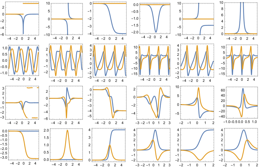
Figure 1: Zero vacuum, $\mathpzc{V}_{0}=\mathcal{J}_{0}=0$, “1-soliton” type of solutions. We plot the fields in eqs. (22)–(25) (columns) against $x$ for $t=0$. Blue line is the real part, orange line is the imaginary part. 1st row: Real (singular) mKdV solution with $\kappa=1$ generates a KdV kink ($\eta^{+}$), a dark soliton ($\mathcal{J}^{+}$), and a peakon ($\mathcal{J}^{-}$); changing $\mathcal{J}^{\pm}\to-\mathcal{J}^{\pm}$ yields a “focusing” KdV solution. 2nd row: Periodic mKdV solutions ($\kappa=i$). Both $\mathcal{J}^{\pm}$ are called positons. 3rd row: Localized waves with complex $\kappa=1+i$. $\mathcal{J}^{-}$ is a negaton (we shifted $\mathcal{J}\mapsto-\mathcal{J}$) and is reminiscent of the Peregrine soliton. 4th row: Purely imaginary mKdV solution ($\kappa=1$, $f\mapsto f+i\pi/2$), i.e., a kink and a typical soliton, generates coupled kinks and solitons of focusing KdV.

In Fig. 2 we generate a similar classification but with a constant background $\mathpzc{V}_{0}\neq 0$. In the 1st row we have real mKdV dark solitons generating real KdV dark solitons. The 2nd row have similar positons as in the previous figure, but over a constant background. The 3rd row shows KdV negatons over a constant background; the amplitude of $\mathcal{J}^{-}$ is significantly larger than their mKdV analogues. The 4th row illustrates how focusing mKdV solutions generates large amplitude solitons for complex KdV systems, including system (26); this again has similar shape as the Peregrine soliton [3]. Even the mKdV dark soliton has relatively large amplitude.

$\phi$ (mKdV)

$\mathpzc{V}$ (mKdV)

$\eta^{+}$ (KdV)

$\mathcal{J}^{+}$ (KdV)

$\eta^{-}$ (KdV)

$\mathcal{J}^{-}$ (KdV)

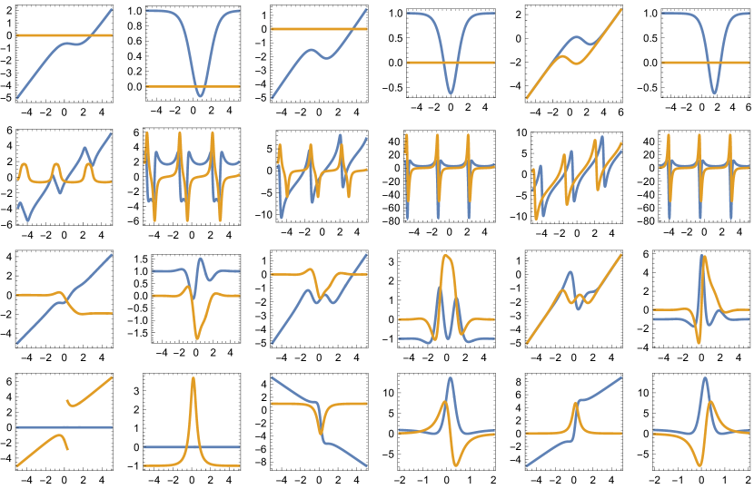
Figure 2: Nonzero vacuum, $\mathpzc{V}_{0}\neq 0$ and $\mathcal{J}_{0}=\mathpzc{V}_{0}^{2}$, “1-soliton” type of solutions. We plot the fields in eqs. (22)–(25) (columns) against $x$ for $t=0$. Blue line is the real part, orange line is the imaginary part. 1st row: $\kappa=0.9$, $\mathpzc{V}_{0}=1$. Real mKdV dark soliton generates real KdV dark soliton. 2nd row: Periodic mKdV solutions, $\kappa=0.9i$, $\mathpzc{V}_{0}=1$. Both $\mathcal{J}^{\pm}$ are positons over a nonzero background. 3rd row: Localized waves, $\kappa=0.9(1+i)$, $\mathpzc{V}_{0}=1$. For $\mathcal{J}^{\pm}$ we shifted the sign, yielding a large focusing KdV wave. 4th row: Purely imaginary mKdV solution, $\kappa=0.9$, $f\mapsto f+i\pi/2$, $\mathpzc{V}_{0}=i$. This generates coupled KdV dark solitons and kinks. $\mathpzc{V}$ has a large amplitude, and $\mathcal{J}^{\pm}$ even more so (they have the profile of a Peregrine soliton).

In Fig. 3 we illustrate complex KdV breathers of system (26). These are obtained from “2-soliton” ($n=2$) mKdV tau functions with complex conjugate wave numbers. Over a zero background, such breathers have a typical amplitude, however over a nonzero background they have large amplitudes and provide a model for rogue waves, as illustrated in the right plot.

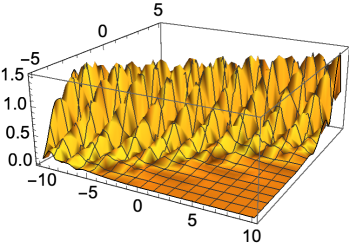
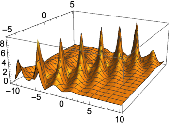
Figure 3: Complex KdV breathers. “2-soliton” solution (see eqs. (22)–(25)) with $\kappa_{1,2}=0.2\pm 0.95i$ and a phase $i\pi/2$ in $f$. These come from purely imaginary solutions of the mKdV hierarchy. Left: Zero vacuum, $\mathpzc{V}_{0}=0$. Right: Constant vacuum, $\mathpzc{V}_{0}=i$; note the large amplitude of this breather, which is a rogue wave.

In Fig. 4 we consider a “4-soliton” solution ($n=4$) of the mKdV hierarchy, which induces solutions to system (26); the parameters are indicated in the caption. We generate an extreme localized wave (left plot) even over a zero vacuum. For the same parameters, however over a constant vacuum $\mathpzc{V}_{0}=1$, such waves model extremely violent phenomena (right plot) with rogue waves scattered in several places. By tweaking parameters, it is possible to obtain a localized rogue wave, although with much larger amplitude compared to the zero background case.

4 Conclusion

We have constructed solutions of the (focusing/defocusing) KdV hierarchy in terms of tau functions of the mKdV hierarchy. Such solutions hold for any model of the hierarchy by adapting the dispersion relation, including the specific complex KdV system (26). We have illustrated how rogue waves can be obtained from simple analytical formulas. Our examples are by no means exhaustive, i.e., by suitable combination of elementary mKdV tau function one can construct countless examples of extreme waves and model rich nonlinear phenomena.

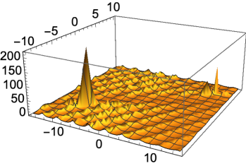
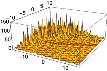
Figure 4: Complex KdV rogue waves. “4-soliton” solution (see eqs. (22)–(25)); $\kappa_{1}=0.1+0.1i$, $\kappa_{2,3}=0.3\pm 0.9i$, $\kappa_{4}=0.91i$, and a phase $i\pi/2$ in $f$. Left: Zero vacuum, $\mathpzc{V}_{0}=0$. Note the large localized rogue wave. Right: Constant vacuum, $\mathpzc{V}_{0}=1$. Note the extremely violent and high amplitude waves. By changing parameters it is possible to create localized waves as in the left figure but with much larger amplitude.

JFG and AHZ thank CNPq and FAPESP for support. YFA thanks FAPESP for financial support under grant 2021/00623-4 and 2022/13584-0. GVL thanks CAPES (finance Code 001).

References

References

• [1] Adans Y F, França G, Gomes J F, Lobo G V and Zimerman A H 2023 J. High Energ. Phys. 2023 160
• [2] Solli D, Ropers C, Koonath P and Jalali B 2007 Nature 450 1054–1057
• [3] Kibler B, Fatome J, Finot C, Millot G, Dias F, Genty G, Akhmediev N and Dudley J M 2010 Nature Phys. 6 790–795
• [4] Baronio F, Degasperis A, Conforti M and Wabnitz S 2012 Phys. Rev. Lett. 109(4) 044102
• [5] Tsai Y Y, Tsai J Y and I L 2016 Nature Phys. 12 573–577
• [6] Dudley J M, Genty G, Mussot A, Chabchoub A and Dias F 2019 Nat. Rev. Phys. 1 675–689
• [7] Gardner C S, Greene J M, Kruskal M D and Miura R M 1967 Phys. Rev. Lett. 19(19) 1095–1097
• [8] Zakharov V E and Shabat A B 1972 Sov. Phys.–JETP 34 62–69
• [9] Drinfel’d V and Sokolov V 1985 J. Math. Sci. 30 1975–2036
• [10] Verosky J M 1991 J. Math. Phys. 32(7) 1733
• [11] Gomes J F, França G S, de Melo G R and Zimerman A H 2009 J. Phys. A: Math. Theor. 42 445204
• [12] Brazhnyi V A and Konotop V V 2005 Phys. Rev. E 72(2) 026616
• [13] Ankiewicz A, Bokaeeyan M and Akhmediev N 2019 Phys. Rev. E 99(5) 050201
• [14] Hu H, Tong B and Lou S 2006 Phys. Lett. A 351 403–412 ISSN 0375-9601