High-Resolution Imaging of a TESS Control Sample: Verifying a Deficit of Close-In Stellar Companions to Exoplanet Host Stars

Abstract

The large number of exoplanets discovered with the Transiting Exoplanet Survey Satellite (TESS) means that any observational biases from TESS could influence the derived stellar multiplicity statistics of exoplanet host stars. To investigate this problem, we obtained speckle interferometry of 207 control stars whose properties in the TESS Input Catalog (TIC) closely match those of an exoplanetary host star in the TESS Object of Interest (TOI) catalog, with the objective of measuring the fraction of these stars that have companions within $\sim 1.2"$. Our main result is the identification of a bias in the creation of the control sample that prevents the selection of binaries with $0.1"\lesssim\rho\lesssim 1.2"$ and $\Delta$mag $\lesssim 3$. This bias is the result of large astrometric residuals that cause binaries with these parameters to fail the quality checks used to create the TIC, which in turn causes them to have incomplete stellar parameters (and uncertainties) in the TIC. Any stellar multiplicity study that relies exclusively upon TIC stellar parameters to identify its targets will struggle to select unresolved binaries in this parameter space. Left uncorrected, this selection bias disproportionately excludes high-mass-ratio binaries, causing the mass-ratio distribution of the companions to deviate significantly from the uniform distribution expected of FGK-type field binaries. After accounting for this bias, the companion rate of the FGK control stars is consistent with the canonical 46$\pm$2% rate from Raghavan et al. (2010), and the mass-ratio distribution agrees with that of binary TOI host stars. There is marginal evidence that the control-star companions have smaller projected orbital separations than TOI host stars from previous studies.

1 Introduction

The ever-growing tally of exoplanets discovered by the Transiting Exoplanet Survey Satellite (TESS; Ricker et al., 2015) has led to great interest in these planets’ host stars, particularly those that harbor stellar companions. Even beyond its intrinsic astrophysical implications for planet formation, the presence of a companion star can result in a number of biases, ranging from the systematic underestimation of planetary radii (Ciardi et al., 2015) to the miscalculation of exoplanet occurrence rates (Hirsch et al., 2017; Bouma et al., 2018).

The presence of a stellar companion can profoundly influence the process of planet formation. For example, Kraus et al. (2012) found that the presence of a close ($\lesssim 40$ AU) stellar companion causes protoplanetary disks to be dispersed much faster ($\lesssim 1$ Myr) than in wide binaries or single stars ($1-3$ Myr), leading to a deficit of planets in those systems in comparison to single stars. And in a high-resolution-imaging study of 382 Kepler Objects of Interest (KOIs), Kraus et al. (2016) determined that planets are underabundant by a factor of $\sim 3$ in binaries with separations $\lesssim 50$ AU (at $4.6\sigma$ significance). At wider separations, Kraus et al. (2016) found little evidence of suppression, a result somewhat at odds with Wang et al. (2014), who concluded ( with 1-2$\sigma$ significance) that the suppression of circumstellar planets extends to stellar binary separations as wide as $\sim$1500 AU for Kepler based on adaptive-optics imaging and radial velocity analysis of a sample of KOIs. Despite this mild disagreement about planet suppression at large binary separations, both Wang et al. (2014) and Kraus et al. (2016) concur that planet suppression is most pronounced at small binary separations. Further, Hirsch et al. (2021) found that the occurrence rate of giant planets in widely separated ($100$ AU) binaries was identical to that of single stars, while in close binaries ($<100$ AU), it was reduced by a factor of $4-5$. In line with this picture, a series of studies, including Ziegler et al. (2020), Howell et al. (2021), and Lester et al. (2021), used high-contrast imaging to find that exoplanet-hosting TESS Objects of Interest (TOIs) show a deficit of stellar companions within 100 AU in comparison to field binaries.

As work progresses on TOI host stars, a subtle question arises: to what extent might the differences with respect to field binaries be attributable to observational biases? Ziegler et al. (2020), Howell et al. (2021), and Lester et al. (2021) compared the properties of binary TOI host stars against the properties of FGK dwarfs from Raghavan et al. (2010). Although a volume-limited study like Raghavan et al. (2010) should combat observational biases in order to yield statistically robust results for stellar populations, Stassun et al. (2018) pointed out that the main scientific objective of TESS is to maximize the number of small planets detected via the transit method—and not to yield a statistically unbiased representation of the population of extrasolar planetary systems. It is therefore unclear whether binary statistics derived from Raghavan et al. (2010) provide the best point of comparison for TESS exoplanet hosts.

Comparing the binary rates of transiting planet host stars to the solar neighborhood sample from Raghavan et al. (2010) makes the implicit assumption that the there are no systematic differences between the TOI sample and the volume limited solar neighborhood sample. For example, the planet content of the Raghavan et al. (2010) sample is not well characterized. Toward the goal of trying to compare the binarity rate of TOIs to that of the general field, we have constructed a control sample of stars observed by TESS but not found to host transiting exoplanets. The planetary abundance of these control stars is unknown but it is known that no close-in transiting planets have been detected around them. Our aim was to use this control sample to see whether its binarity rate was systematically different than the binarity rate of stars found to host close-in transiting planets, as seen by the same instrument (TESS).

In the process of conducting this experiment, we discovered a bias in the TESS Input Catalog whereby well-characterized stars (e.g., stars with complete and reliable stellar parameters) are preferentially single stars. In this paper, we describe the selection of the control sample and the discovery of the bias. We have worked to correct for this bias and make a true assessment of the binarity rate of FGK stars that were observed with TESS and found to not host a close-in transiting planet.

2 Data

2.1 Selection of control stars

Our objective was to pair individual TOIs with a non-TOI control star of comparable $T_{eff}$, radius, and distance. We excluded from consideration TOIs with a TFOPWG disposition of “FP” (false positive). For each of the remaining TOIs, we searched version 8.2 (Paegert et al., 2021) of the TESS Input Catalog (TIC) for stars with similar effective temperature ($T_{eff}$), radius, and distance relative to each specific TOI. This left us with a large, preliminary list of candidate control stars for each TOI. To identify the closest matches for any given TOI, we added in quadrature the fractional differences in $T_{eff}$, stellar radius, and distance between that particular TOI and the candidate control star. The resulting metric enabled us to create a ranked list of suitable control stars for each TOI.

We eliminated any control stars that were candidate exoplanet hosts, and we also imposed a requirement that they have been observed by TESS in at least one sector. This restriction provided some confidence that the control stars lack detectable transiting exoplanets. The non-detection of candidate exoplanets by TESS does not establish that these stars lack exoplanetary systems; TESS can detect exoplanets only if (1) their orbital inclinations are sufficiently high to result in a transit of the host star, (2) the transits occur during the TESS observing window, and (3) the transit depth is sufficiently deep to be detected by the analysis pipeline. However, our goal was to compare TOI stars against otherwise identical non-TOI stars.

The TIC v.8.2 stellar parameters are foundational to our methodology, so it is worthwhile to briefly summarize their provenance, which Stassun et al. (2019) explain in meticulous detail. The TIC v.8.2 computes stellar parameters for stars with good Gaia DR2 astrometry and photometry. For the stars that survive this initial cut, $T_{eff}$ is systematically calculated from the dereddened Gaia DR2 colors of each star except in special cases where a spectroscopic $T_{eff}$ is available. Given the $T_{eff}$ and the Gaia DR2 distance, the stellar radius is calculated by applying the Stefan-Boltzmann relation. Stassun et al. (2019) caution that these calculations make no allowance for the reality that some apparently single stars are actually unresolved binaries and that the presence of a companion can cause the computed stellar parameters to be unreliable. For example, if an unresolved binary contained two identical stars, the stellar radius could be overestimated by a factor of $\sqrt{2}$. Additionally, for some specially curated lists of targets, the stellar parameters therein supersede the parameters computed by the TIC pipeline.

2.1.1 Comparison of control stars to TOIs

The histograms in Figure 1 confirm that the observed control stars closely match the properties of their corresponding TOI stars, with only small fractional differences in the effective temperature, radius, and distance. The control stars span a wide range of effective temperature along the main sequence, as established in Figure 3.

We also investigated whether the observed TESS magnitudes of the control stars agree with those of the TOIs. While this was not explicitly controlled for in our selection, we would expect the magnitude differences to be similar because in the absence of interstellar extinction, the stellar effective temperature, radius, and distance should determine, via the Stefan-Boltzmann relation, the apparent magnitude.

The resulting distribution is symmetric and centered on 0, with over 90% of the differences being smaller than 0.2 mag, which is reassuring. Nevertheless, there were four extreme outliers where the TOI and control stars had magnitude differences greater than 1 magnitude. We used the Green et al. (2019) three-dimensional interstellar reddening maps to investigate these outliers, and in each case, there were significant differences in the interstellar extinction along the two lines of sight. Although the computation of the TESS magnitude does apply a correction for extinction (Stassun et al., 2019), we suspect that the four TOI-control star pairings with large magnitude differences might be the result of an imperfect dereddening that propagated into the computations of the TESS magnitude, $T_{eff}$, and the stellar radius.

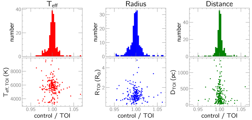
Figure 1: Comparison of effective temperature, stellar radius, and distance between each observed control star and its corresponding TOI. The abscissa in each panel is the fractional difference between a control star’s property and that of the TOI.

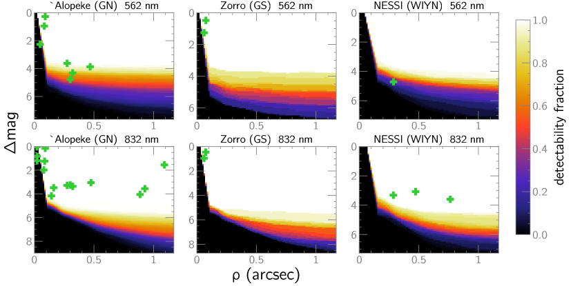
Figure 2: Two-dimensional histograms of the contrast curves used in this study, separated by instrument and bandpass. Detected companions within $\rho<1.2"$ are marked with green crosses. Companions detected at wider separations (six at 832 nm and two at 562 nm) are not shown. Many of the companions detected at 832 nm were undetected at 562 nm. The color scale represents the fraction of contrast curves in which a companion could have been detected at a given combination of $\rho$ and $\Delta$mag. Note that the range of $\Delta$mag varies between the panels because the contrast curves vary from from instrument to instrument.

2.2 Observational technique

Our observations were carried out with the ‘Alopeke and Zorro speckle cameras (Scott et al., 2021) on the 8-meter Gemini North and Gemini South telescopes, respectively. ‘Alopeke and Zorro are identical instruments. Each contains a dichroic, positioned at a $45^{\circ}$ angle relative to the collimated input beam, to split the beam into blue ($\lambda<674$ nm) and red ($\lambda>674$ nm) components. Each beam travels to its own dedicated electron-multiplying CCD camera, so both ‘Alopeke and Zorro obtain simultaneous dual-band observations with a field of view of $2.5"\times 2.5"$. To boost the contrast of the speckles, our observations utilized narrow-band filters, centered at 562 nm (44 nm FWHM) and 832 nm (40 nm FWHM) for the blue and red cameras, respectively.

Speckle observations with these instruments were obtained in sets of 1000 consecutive frames, each with an exposure time of 60 milliseconds with negligible overhead. Depending on the brightness of the target and the sky conditions, we typically obtained anywhere from 3 to 15 sets. Some of our observations were obtained using the 3.5-m WIYN telescope and the NN-EXPLORE Exoplanet Stellar Speckle Imager (NESSI; Scott et al., 2018) instrument, which is conceptually similar to (and served as the prototype for) both ‘Alopeke and Zorro. The NESSI observations used the same filters as the Gemini observations, but the resolution is worse by a factor of $\sim 2$ because of the smaller aperture.

Within a short time of each observation of a control star, we obtained speckle observations of a bright, single star within a few degrees of the control star in order to measure the speckle transfer function. We reduced the data to obtain high-level data products using a pipeline described in Howell et al. (2011). For any detected companion stars, we measured the angular separation and position angle relative to the primary target along with the magnitude difference. Another pipeline product is a reconstructed image of the focal plane centered on the target. From this, we measured a contrast curve that represents the flux corresponding to a 5$\sigma$ deviation from the mean within each of a set of concentric annuli centered on the target star. This contrast curve is smoothed slightly to remove deviations caused by known artifacts or the flux from a detected companion. The contrast curve is estimated out to a maximum separation of 1.2”, a limit that avoids problems caused by potential centering errors of the target within the readout section of the detectors and the loss of photometric sensitivity at wider separations where speckle patterns can start to become uncorrelated. ‘Alopeke (Gemini North) and Zorro (Gemini South) generally achieve better contrast than NESSI, and for all instruments, the 832 nm filter tends to have deeper contrast limits than the simultaneous 562 nm data.

To measure the pixel scale and the position angle of the detectors, we periodically observe known binary stars whose orbital elements are listed in an updated version of the Hartkopf et al. (2001) catalog. The pixel scale and array orientation are calculated for each observing run, and while they tend to be quite stable between observing runs, we updated them as needed.

3 Results

3.1 Companions to Control Stars

We observed a total of 207 control stars, of which 26 had detected binary companions at 832 nm and 12 had companions at 562 nm (Figure 2). Of these companions, 20 had angular separations of $\rho<1.2"$ at 832 nm with respect to the primary star, while 10 of the companions detected at 562 nm satisfied $\rho<1.2"$.

Table 1: Properties of detected companions to control stars

TIC ID	$\rho$ (arcsec)	$\Delta\mathrm{mag}$	$\theta$ (deg)	$\rho$ (arcsec)	$\Delta\mathrm{mag}$	$\theta$ (deg)
	(832 nm)	(832 nm)	(832 nm)	(562 nm)	(562 nm)	(562 nm)
372086900	0.021	0.02	208.19
377058463	0.022	0.83	241.739	0.048	2.26	240.839
196383895	0.023	1.2	296.698
296781193	0.061	0.96	183.573	0.062	1.26	183.993
437327600	0.075	0.46	202.852	0.076	0.48	202.663
14899687	0.079	1.98	265.021
301482228	0.086	1.24	63.579	0.083	0.95	65.537
267686220	0.091	0.15	243.797	0.091	0.27	243.622
264485499	0.143	4.17	358.335
355691670	0.162	3.48	335.28
85274754	0.275	3.28	125.126	0.275	3.62	125.507
354442089	0.286	3.32	232.234	0.288	4.71	233.203
194461161	0.301	3.25	102.956	0.301	4.77	102.512
91277756	0.322	3.36	18.95	0.321	4.31	18.496
376688975	0.473	3.08	22.114
269390255	0.475	3.05	149.225	0.468	3.87	148.478
83958546	0.764	3.6	245.005
301482610	0.887	4.05	338.992
241257501	0.927	3.56	327.102
96876685	1.091	1.55	203.39
140343515	1.218	5.13	317.466
716026635	1.312	3.73	314.706
91597865	1.319	2.81	60.841	1.331	2.8	62.032
2100594	1.689	9.99	323.692
306125356	1.725	5.0	70.136
411551642	2.101	2.35	353.914	2.085	3.61	354.409

To assess whether any of the apparent companions might be unrelated stars along the line of sight to the primary, we retrieved a list of all cataloged TIC v.8.2 stars within a radius of 15 arcmin centered on each control star with a detected companion; built upon Gaia DR2, the TIC v.8.2 is complete to well below the limiting magnitude of our observations. Within this search region, we counted the number of stars within $\pm$1 mag of the detected companion. This yielded a localized estimate of the number density of sources of comparable brightness to the putative companion, which lets us estimate the probability of a chance alignment that causes a physically unrelated field star to masquerade as an apparent companion. We found that there is very little chance that any of the detected companions are physically unrelated alignments. In some cases, there were no field stars of comparable brightness to the putative companion; at the opposite extreme, the control-star companion in the densest star field had a line-of-sight probability of just $0.2\%$. We conclude that all 26 companions are probably physically associated with their control stars, a finding that is consistent with previous analyses about the likelihood of boundedness of close-in companions (e.g., Everett et al., 2015; Hirsch et al., 2017).

Table 1 lists the properties of the detected companions, while Table 2 provides the correspondence between the control stars and TOIs.

3.2 Simulations of Binary Companions

It is straightforward to describe the properties of the companions that we observed around the control stars. But for the apparently single control stars, the absence of a detected companion might mean that a control star is single, that any companions are too faint to be detected, or that the binary angular separation might be extremely small or too large to fit inside the speckle field of view. Speckle interferometric studies by Matson et al. (2019) and Howell et al. (2021) addressed these issues by calculating three separate fractions. The first, the “companion fraction,” estimates the fraction of all plausible companions whose $\Delta$mag would be above the contrast limits (“the companion fraction”). The second is the fraction of semimajor axes that would cause the companion’s angular separation to be within the instrument’s field of view (“the distribution fraction”). Finally, the “speckle fraction” is the product of the companion and distribution fractions, and it estimates the percentage of companions that would be detectable with speckle observations.

To calculate the speckle fraction for each star in our control sample, as well as the predicted distributions for the mass ratio and the binary separations, we use a Monte Carlo simulation similar to the ones designed by Ziegler et al. (2020) and Lester et al. (2021). For each control star, we retrieve its mass and distance, as well as their associated uncertainties, from the TIC. Each iteration of the simulation then proceeds as follows. We add Gaussian noise to both the stellar mass and distance and randomly draw a binary mass ratio $q$ from the Raghavan et al. (2010) distribution, which has a uniform probability for $0.2\leq$ q $\leq 0.95$, with a doubled probability above q=0.95. We further draw a random orbital period from the Raghavan et al. (2010) log-normal distribution of $\log P=5.03$ d, $\sigma_{\log P}=2.28$.

Given the two stellar masses and their orbital period, we calculate their semimajor axis. We then randomly draw from uniform distributions the binary inclination, argument of periastron, longitude of the ascending node, and orbital eccentricity. With these simulated orbital elements, we calculate the angular separation of the synthetic binary companion at a random orbital phase. We also calculate $\Delta$ mag in both the $V$ and TESS bandpasses based on the stellar masses and the Modern Mean Stellar Dwarf Sequence (MMSDS; Pecaut & Mamajek, 2013).

To determine whether the simulated companion would be detectable with our observations, we retrieve the observed contrast curve for the control star, which shows the 5$\sigma$ limit for $\Delta$mag as a function of the angular separation $\rho$. If the simulated companion is above the contrast curve and within 1.2” of the control star, we classify it as detected; otherwise, we classify it as a non-detection.

We impose the upper limit of 1.2” because it is the limit of the parameter space examined in the contrast curves; above this separation, speckles can become decorrelated (Horch et al., 2011). Nevertheless, binaries with wider separations are occasionally detected by our pipeline, which contradicts the assumption in our simulations that companions are undetectable when $\rho>1.2$ arcsec.

Since the FGK binary parameters from Raghavan et al. (2010) cannot be extrapolated to other spectral types (e.g., M-dwarfs; Winters et al., 2019), we further limit the simulations to those systems with FGK-type primary stars (estimated from their effective temperatures in the TIC). Fifteen companion-harboring systems in our control sample satisfy the spectral-type and angular-separation constraints.

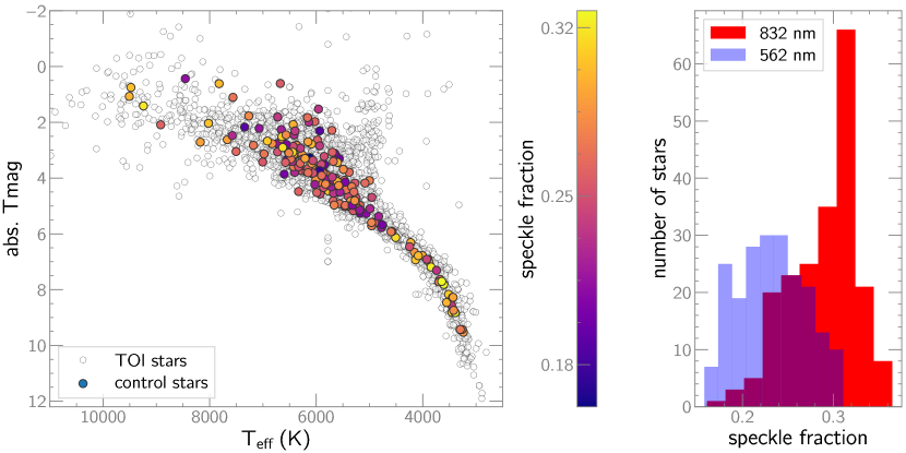
Figure 3: Left: Color-magnitude diagram of the control-star sample compared to that of all TOIs (white circles), showing the absolute TESS magnitude as a function of effective temperature. The color of each control-star marker indicates the 832 nm speckle fraction, defined as the fraction of possible companions that could be detected in that bandpass based on our contrast limits, the instrument field of view, and the Raghavan et al. (2010) binary parameters. Right: Histograms of the speckle fraction for each bandpass.

The speckle fraction for each star is simply the fraction of the 1000 simulations that produced a detectable companion, subject to the aforementioned constraints. Figure 3 shows that the speckle fractions for the control sample are uncorrelated with a control star’s location in a color-magnitude diagram, and it further establishes that the speckle fraction tends to be larger at 832 nm than at 562 nm.

One of the main limitations of our simulations is the uncertainty of the contrast curves at separations within $\rho<0.1"$. At larger separations, the limiting magnitude is estimated empirically by calculating a 5$\sigma$ threshold from the minima and maxima in the reconstructed speckle image as a function of $\rho$, but at small radii, simple geometric considerations mean that there are relatively few minima and maxima upon which to estimate a detection threshold. Accordingly, $\Delta$ mag is assumed to be 0 at the diffraction limit and is then linearly interpolated to the beginning of the empirical contrast curve at 0.1 arcsec. However, in good seeing conditions, we occasionally detected companions within $\rho<0.1"$ at values of $\Delta$ mag that are nominally below our detection threshold (Figure 2), raising the prospect that our contrast curves are too pessimistic about the actual capability of ‘Alopeke and Zorro to detect companions at very small separations. Crucially, this issue works in one direction: it will cause genuinely detectable combinations of $\rho$ and $\Delta$ mag to be wrongly classified as undetectable in our simulations. As a result, our simulations likely underpredict the number of detectable companions and therefore provide a lower limit.

The simulations allow us to compute the expected number of detected companions for an assumed orbital-period distribution. To estimate the expected number of detectable companions within 1.2” of FGK stars, we compute the average number of synthetic companions that were detected in the 1,000 simulations. Because there is a companion in each simulation (i.e., a presumed multiplicity rate of 100%), we then multiply by the FGK dwarf multiplicity rate of $46\pm 2$% from Raghavan et al. (2010) to take into account that slightly over half of the FGK dwarfs are expected to be single. This leaves us with a predicted tally of detected companions.

3.3 The absence of close, high-mass-ratio binaries

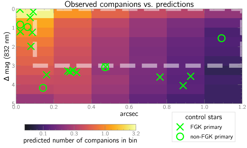
Figure 4: Two-dimensional histogram showing the predicted number of companions for FGK primaries at various combinations of $\rho$ and $\Delta$mag. The color scale is logarithmic. The predictions are from Monte Carlo simulations that use Raghavan et al. (2010) field-binary statistics. The 20 control-star companions detected at 832 nm with separations under 1.2” are also shown, revealing the conspicuous absence of detected companions at $0.1"\lesssim\rho\lesssim 1.2$” and $\Delta$mag $\lesssim 3$ (the region bounded with a thick dashed white line). The simulations predict no such deficit, which we show to be the result of a selection bias that prevented the observation of binaries in this parameter space.

The Raghavan et al. (2010) statistics predict that we should have detected $23\pm 3$ companions at 832 nm and $18\pm 3$ at 562 nm around the FGK dwarfs in our sample. For comparison, we found that only 15 FGK control stars had companions within 1.2” at 832 nm (and just 8 at 562 nm), so there is a significant deficit of companions in our observations. This deficit cannot be explained by uncertainty in the contrast curves used in the simulations. As we discussed earlier, the contrast curves within $\rho<0.1"$ underestimate our ability to detect close-in companions in good seeing, and since our simulations predict that there should be many companions within $\rho<0.1"$, the totals predicted by our simulations are a lower limit.

Fig. 4 shows a two-dimensional histogram of the expected detection rate of synthetic companions as a function of both $\rho$ and $\Delta$mag, and to facilitate a direct comparison against the observations, it also plots $\rho$ and $\Delta$mag for all companions detected at 832 nm. This comparison reveals a striking disagreement between the simulations and observations. In particular, not a single observed companion to an FGK star has $0.1"\leq\rho\leq 1.2"$ and $\Delta$mag$<3$, even though the simulations predict this to be a fertile region for finding companions. Indeed, our simulations predicted an average of $9\pm 2$ companions with $0.1"\leq\rho\leq 1.2"$ and $\Delta$mag$<3$; the minimum number of predicted companions in this parameter space was 4.

The absence of observed companions with $0.1"\leq\rho\leq 1.2"$ and $\Delta$mag$<3$ for FGK stars is a stark deviation from the properties of Raghavan et al. (2010) field binaries, and taken at face value, it would conflict with a line of studies of stellar multiplicity surveys of transiting-exoplanet host stars. However, we show in Sec. 3.4 that this surprising deficit is attributable to a selection bias in the creation of the control sample.

3.4 Origin of the bias

The control stars were selected based on their stellar parameters in the TIC (specifically, their effective temperatures, radii, and distances), as well as the uncertainties of these parameters. However, before stellar parameters are calculated in the TIC workflow, two preliminary tests of the quality of the Gaia DR2 astrometry and photometry are performed; if a source passes both tests, it is assigned a Gaia quality flag (gaiaqflag) of 1; if the source fails one or both tests, then gaiaqflag = 0.

Although verifying the caliber of the astrometry and photometry might sound innocuous and even desirable, this process has deleterious consequences for close binaries. Previous studies (e.g., Deacon & Kraus, 2020; Ziegler et al., 2020) have already established that Gaia astrometry of close, unresolved binaries tends to have large residuals, quantified by the renormalized unit weight error statistic (RUWE). Indeed, the RUWE can be well over an order of magnitude larger for binaries with separations of $0.1"\lesssim\rho\lesssim 1"$ and magnitude differences $\lesssim 2$ mag (Fig. 4 in Ziegler et al., 2020). As a result, quality cuts made on astrometry will penalize unresolved binaries in that parameter space, causing these systems to be disproportionately excluded in comparison to single stars, widely separated binaries, extremely close binaries ($\rho<0.1"$), and binaries with very large $\Delta$ mag.

To be clear, when a source fails either of the Gaia quality tests (i.e., gaiaqflag = 0), it is still included in the TIC. But the stellar parameters of these sources tend to be incomplete and/or lack uncertainties compared to sources that pass the quality tests (gaiaqflag = 1). This is because the TIC automatically computes stellar parameters only if gaiaqflag = 1. While stars with gaiaqflag = 0 might have stellar parameters and uncertainties, this happens only if they were obtained from other sources, such as spectroscopic catalogs or specially curated lists. Thus, by requiring the control stars to have valid $T_{eff}$, radii, and distances (along with uncertainties on each parameter), our selection criteria unintentionally excluded certain types of binaries from the control sample.

3.5 Testing the bias

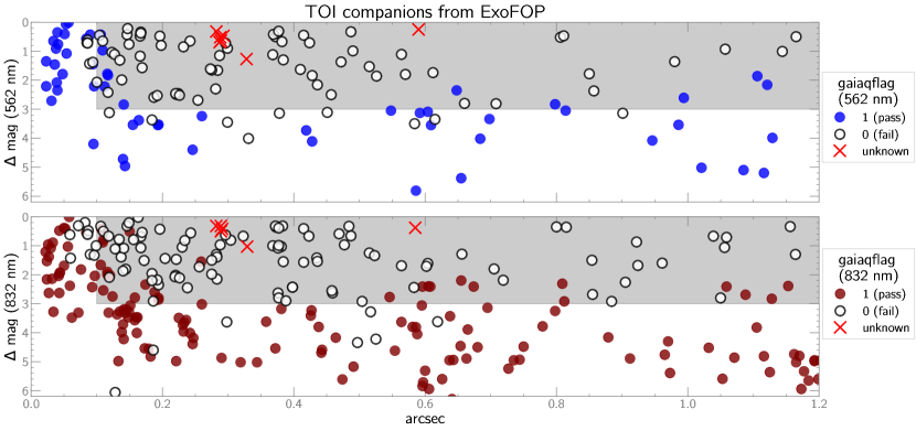
Figure 5: The dependence of gaiaqflag on $\Delta$mag and $\rho$ in companion-hosting TOI objects. Binaries with $\Delta$mag $\lesssim 3$ and $0.1"\lesssim\rho\lesssim 1.2"$ (represented with a shaded region in both panels) disproportionately fail the Gaia quality test. As we discuss in the text, sources that fail the Gaia quality test will lack the parameters used to assemble our control sample, creating a powerful selection bias against binaries within this parameter space.

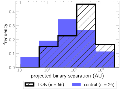
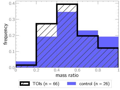
Figure 6: Top: Projected binary separations for the detected companions in the control sample compared against those of the Howell et al. (2021) and Lester et al. (2021) TOI stars whose values of $\rho$ and $\Delta$mag place them outside the parameter space of the selection bias. A K-S test comparing these two distributions has a $p$-value of 0.07, indicating marginal statistical evidence of a difference. Bottom: As with the top panel, except that mass ratios are compared. The corresponding K-S test has a $p$-value of 0.2, indicating no statistically significant difference. In both panels, we lift the restrictions on spectral type and $\rho$ used in the simulations, so all 26 detected companions around control stars are included.

As a test of this scenario, we downloaded from the ExoFOP database a list of speckle-detected companions to TOI stars at 562 nm and 832 nm (ExoFOP, 2019). Figure 5 plots $\Delta$mag as a function of $\rho$ for these companions and uses different marker styles to illustrate the dependence of gaiaqflag on both $\rho$ and $\Delta$mag. Consistent with Deacon & Kraus (2020) and Ziegler et al. (2020), the stars with companions within $0.1"\lesssim\rho\lesssim 1"$ and $\Delta$ mag (832 nm)$\lesssim 2$ overwhelmingly show gaiaqflag = 0. This result holds for companions detected at 562 nm, except that the sources with gaiaqflag = 0 extend to $\Delta$mag (562 nm)$\lesssim 3$.

The next step in assessing the impact of this bias is to examine the impact of gaiaqflag = 0 on our selection criteria. To that end, we inspected the TIC parameters of the companions shown in Figure 5 to assess whether they differ depending on the value of gaiaqflag. Almost every source with gaiaqflag = 1 had valid parameters and uncertainties for the stellar radius, effective temperature, and distance. However, a very different picture emerges for the sources with gaiaqflag = 0, of which only 42% had estimates for all three of those parameters. Moreover, none of the gaiaqflag = 0 sources had valid uncertainties for all three of those parameters. The combination of incomplete TIC parameters and missing uncertainties means that it would be difficult or even impossible to select these stars for observation based solely on the criteria used to assemble the control sample.

3.6 Impact of the bias

The selection bias described above is insidiously subtle because it is caused by the combination of the TIC’s quality-control tests and our relatively stringent selection criteria. In particular, it would normally seem reasonable to require, as we did, that sources have uncertainties on their stellar parameters, and we expect that this selection bias will afflict studies that select their targets based solely on their stellar parameters and their associated uncertainties in the TIC. With this in mind, it is worth considering how this bias could distort the scientific interpretation of the data.

Left uncorrected, this selection bias might lead to the unwarranted conclusion that the FGK control stars have a much lower companion fraction than the canonical value of $46\pm 2\%$, based on the simple fact that simulations using Raghavan et al. (2010) statistics significantly overpredict the number of observed companions. However, this deficit disappears once the simulations are modified to simulate the selection bias. After adjusting our simulations to disallow the creation of binaries with $0.1"\leq\rho\leq 1.2"$ and $\Delta$mag $<3$ mag, we would expect to find, within 1.2”, $14.7\pm 2.3$ companions at 832 nm and $10.7\pm 2.0$ at 562 nm, assuming a 46$\pm$2% multiplicity rate from Raghavan et al. (2010). These predictions are in remarkably good agreement with the observed totals of 15 and 8 for those respective bandpasses. In short, the observed companion rate of the FGK control stars within 1.2” and $\Delta$mag $<3$ mag agrees with the Raghavan et al. (2010) statistics.

Likewise, the FGK dwarfs in the control sample show an apparent enhancement of binaries with q$\sim$0.5 (Figure 6), a feature that is inconsistent with the Raghavan et al. (2010) mass-ratio distribution. But here again, the selection bias is responsible for this apparent feature. When both components of a binary are on the main sequence and have similar masses, they will have similar luminosities and hence a small $\Delta$mag, making them vulnerable to this selection bias if their angular separations are wider than 0.1”. Conversely, unequal-mass binaries will have larger $\Delta$mag, causing them to be overrepresented in our control sample.

3.7 Properties of detected binaries

Due to the potency of this selection bias (Figure 4 and Figure 5), we can perform only a limited comparison between the control-sample binaries and companions to TOIs. We took TOI binaries from Howell et al. (2021) and Lester et al. (2021) and excluded those with $0.1"\leq\rho\leq 1.2"$ and $\Delta$mag $<3$ mag in order to mimic the selection bias that afflicts the control sample. The upper panel in Figure 6 presents a histogram of the projected separations of the FGK stars in the control sample, compared to the TOI binaries from Howell et al. (2021) and Lester et al. (2021), while the lower panel compares their mass ratios. In both comparisons, we used a Kolomogorov-Smirnoff (K-S) test to evaluate how different the two distributions are from each other. The $p$-value of the K-S test indicates the statistical significance of the difference in the compared distributions, with largest significance for the smallest values of $p$ ($p=0.00$–$0.01$). The $p$-value for the mass-ratio comparison is 0.2, suggesting no significant difference between the control-star and TOI mass ratios subject to the aforementioned constraints. However, there is modest evidence ($p$ = 0.07) for a difference in the projected separations of the control stars and binary TOIs. Figure 6 shows that the TOI companions have wider separations than the control-star companions; if true, this would be consistent with earlier findings (e.g. Howell et al., 2021; Lester et al., 2021) that exoplanet-hosting TOI binaries have wider separations than field binaries.

3.8 Statistical significance

Our sample size (n = 207) is relatively small compared to the $>5000$ TOIs at the time of writing, and the selection bias described earlier complicates comparisons between the control sample and the corresponding TOIs. For example, if the FGK control stars’ multiplicity rate or binary separations varied dramatically from the Raghavan et al. (2010) statistics, would we be able to tell using the available data?

We used our simulations to explore this issue in several ways. First, we tried predicting the number of detectable companions using the orbital period distribution from Lester et al. (2021). That study found that companions to TOI host stars had wider binary separations than field stars and reported a log-normal orbital-period distribution with $\mu=6.2$ d and $\sigma=1.2$. We reran our simulations using this orbital-period distribution while disallowing the creation of binaries that would be subject to the selection bias. The Lester et al. (2021) distribution predicted $19.3\pm 2.6$ red and $12.1\pm 2.3$ blue companions to FGK stars within 1.2”. For reference, the observed totals were 15 and 8, respectively, so the Lester et al. (2021) period distribution overpredicts the number of companions in both filters.

Although 18 M-dwarfs were included in our control sample, we find this number to be too small for useful statistical inference. Three of those stars (all M1.5 or earlier) harbor companions. Following Clark et al. (2022), we adjusted our simulations to use the Duchêne & Kraus (2013) orbital-period distribution for M-dwarf companions, a flat mass-ratio distribution, and a 27% multiplicity fraction. Using these statistics, our simulations predicted $1.4\pm 0.5$ red companions and $1.1\pm 0.5$ blue companions, accounting for the selection bias in our study. At face value, this would seem to be somewhat at odds with the lack of close-in companions identified by Clark et al. (2022) in their high-resolution imaging of M-dwarf TOIs.

However, it is worth remembering that we estimate spectral types by comparing the effective temperatures reported in the TIC with the Pecaut & Mamajek (2013) sequence. The TIC’s effective temperatures have uncertainties that propagate to the inferred spectral type, and in the case of early M stars, this means that we cannot rule out the possibility that they are late K stars that have been erroneously excluded from our analysis of the FGK control stars. For example, for one of our control stars (TIC 296781193), $T_{eff}=3882\pm 157$ K, and while the inferred spectral type from Pecaut & Mamajek (2013) is M0, the uncertainty means that the spectral type could be as early as K8 or as late as M0.5. The other two M-dwarfs with companions are similarly close to the threshold between spectral types M and K. Thus, the nominal tally of three companions to M-dwarfs in the control sample is rather uncertain.

4 Conclusion

We obtained speckle observations of 207 stars selected because their effective temperature, radius, and distance in the TIC closely resemble the parameters of a corresponding TOI. Our goal was to create a control sample for TOIs in order to assess whether the occurrence rate and properties of stellar companions to TOIs differ from otherwise identical stars that are not known (or suspected) to host short-period transiting exoplanets.

We identified a significant selection bias against the inclusion of certain types of close binaries during the creation of the control sample. The bias occurs because the presence of an unresolved companion causes a source in the TIC to fail preliminary quality tests if the binary separation is in the range $0.1"\lesssim\rho\lesssim 1.2"$ and $\Delta$mag $\lesssim 3$ mag. Sources that fail the TIC quality test tend to have incomplete stellar parameters and often lack uncertainties on the available stellar parameters, so normally uncontroversial selection criteria can have the unintended effect of systematically excluding these close, unresolved binaries. Since this bias is the result of target-selection criteria that rely solely upon TIC stellar parameters and uncertainties, it can be mitigated by using selection criteria based on other sources, and this would be a worthy objective for an improved control sample.

After accounting for this selection bias, our simulations using Raghavan et al. (2010) binary statistics for field FGK stars correctly predicted the number of companions that we detected around our control stars. Moreover, we found that the mass-ratio distribution of the control-star companions agrees with that of binary TOI host stars whose $\rho$ and $\Delta$mag place them outside the parameter space of the selection bias. After correction for the bias introducted into the control sample, we still find modest evidence that the physical separation of binary stars in TOIs is wider than the physical separation of binary components in transiting planet host stars.

Table 2: Correspondence between TOIs and control stars

TIC ID	TOI	Binary	Distance (pc)		Radius (R⊙)		$T_{eff}$ (K)
(control star)		(control star)	control	TOI	control	TOI	control	TOI
194461161	280	B	99.95$\pm$0.95	99.66$\pm$0.30	0.787$\pm$0.037	0.783$\pm$0.039	5410$\pm$110	5450$\pm$190
301482610	297	B	455.3$\pm$5.2	461.5$\pm$5.3	1.123$\pm$0.071	1.09 $\pm$ 0	4960$\pm$120	4870$\pm$120
196383895	518	B	161.0$\pm$1.6	159.8$\pm$1.2	1.132$\pm$0.059	1.14$\pm$0.15	5610$\pm$130	5600$\pm$190
377058463	586	B	256.6$\pm$4.1	253.0$\pm$2.5	2.387$\pm$0.070	2.420$\pm$0.070	9510$\pm$150	9510$\pm$180
264485499	692	B	483$\pm$22	482$\pm$19	2.68$\pm$0.15	2.74$\pm$0.13	9480$\pm$170	9620$\pm$140
376688975	704	B	29.69$\pm$0.13	29.842$\pm$0.024	0.510$\pm$0.015	0.504$\pm$0.015	3690$\pm$160	3625$\pm$69
355691670	772	B	135.55$\pm$0.74	135.37$\pm$0.96	0.814$\pm$0.040	0.820$\pm$0.050	5170$\pm$100	5180$\pm$180
296781193	833	B	41.31$\pm$0.24	41.715$\pm$0.042	0.617$\pm$0.018	0.603$\pm$0.018	3880$\pm$160	3965$\pm$72
301482228	1493	B	373$\pm$22	371.4$\pm$6.2	2.88$\pm$0.21	2.90$\pm$0.14	6030$\pm$100	6060$\pm$130
354442089	1669	B	110.90$\pm$0.76	111.28$\pm$0.37	1.080$\pm$0.066	1.070$\pm$0.050	5540$\pm$140	5550$\pm$130
411551642	1805	B	142.76$\pm$0.81	142.85$\pm$0.43	0.843$\pm$0.046	0.860$\pm$0.040	5260$\pm$120	5230$\pm$110
85274754	1966	B	255.1$\pm$6.6	254.2$\pm$3.2	2.29$\pm$0.10	2.31$\pm$0.10	6430$\pm$100	6390$\pm$260
372086900	2049	B	547.9$\pm$8.4	571.5$\pm$9.0	4.78$\pm$0.22	3.48$\pm$0.21	6670$\pm$180	6050$\pm$150
83958546	2101	B	178.1$\pm$2.3	178.43$\pm$0.59	0.998$\pm$0.046	1.000$\pm$0.050	5640$\pm$100	5620$\pm$130
269390255	2166	B	346.3$\pm$9.3	348.6$\pm$3.5	1.98$\pm$0.10	1.990$\pm$0.090	6570$\pm$170	6520$\pm$120
716026635	2193	B	338.2$\pm$7.2	337.1$\pm$2.4	1.205$\pm$0.057	1.197$\pm$0.055	6190$\pm$150	6080$\pm$130
2100594	2196	B	260.3$\pm$3.6	259.9$\pm$2.0	1.028$\pm$0.051	1.029$\pm$0.050	5720$\pm$160	5730$\pm$130
91277756	2458	B	112.1$\pm$2.3	112.96$\pm$0.54	1.333$\pm$0.066	1.330$\pm$0.060	6080$\pm$150	6090$\pm$120
306125356	2523	B	166.0$\pm$1.4	166.3$\pm$1.0	1.115$\pm$0.060	1.120$\pm$0.050	5790$\pm$130	5810$\pm$270
267686220	3159	B	427$\pm$27	428.1$\pm$5.3	1.82$\pm$0.15	1.810$\pm$0.090	5700$\pm$120	5730$\pm$130
91597865	3415	B	1048$\pm$67	1053$\pm$38	2.54$\pm$0.19	2.56$\pm$0.15	5940$\pm$140	5940$\pm$120
14899687	3755	B	320.5$\pm$5.3	322.4$\pm$3.0	1.074$\pm$0.055	1.080$\pm$0.060	5350$\pm$110	5350$\pm$320
241257501	4244	B	770$\pm$77	768$\pm$21	1.61$\pm$0.18	1.61$\pm$0.10	6300$\pm$130	6310$\pm$200
437327600	4305	B	159.2$\pm$2.3	159.01$\pm$0.82	2.79$\pm$0.13	2.75$\pm$0.12	6160$\pm$140	6200$\pm$130
140343515	4441	B	628$\pm$18	627$\pm$11	1.990$\pm$0.087	1.998$\pm$0.083	7340$\pm$220	7310$\pm$130
96876685	5528	B	103.82$\pm$0.42	101.63$\pm$0.37	0.546$\pm$0.016	0.515$\pm$0.015	3610$\pm$160	3690$\pm$160
416670433	173		151.8$\pm$1.2	152.02$\pm$0.64	1.465$\pm$0.074	1.470$\pm$0.060	6440$\pm$470	6410$\pm$200
247873150	201		113.79$\pm$0.70	113.83$\pm$0.35	1.308$\pm$0.056	1.330$\pm$0.060	6460$\pm$160	6462$\pm$83
437761325	209		113.27$\pm$0.66	113.39$\pm$0.27	0.742$\pm$0.051	0.743$\pm$0.050	4900$\pm$130	4890$\pm$180
101831762	214		39.120$\pm$0.043	38.960$\pm$0.038	0.783$\pm$0.044	0.798$\pm$0.050	5260$\pm$120	5350$\pm$140
23972719	229		211.3$\pm$1.4	211.2$\pm$1.8	0.885$\pm$0.057	0.875$\pm$0.057	5180$\pm$130	5100 $\pm$ 0
238431974	248		75.44$\pm$0.24	75.95$\pm$0.14	1.101$\pm$0.052	1.121$\pm$0.052	5730$\pm$120	5712$\pm$57
65577518	262		43.572$\pm$0.076	43.93$\pm$0.12	0.832$\pm$0.037	0.849$\pm$0.052	5241$\pm$98	5303$\pm$21
9006549	296		465.9$\pm$5.9	471.8$\pm$4.8	0.956$\pm$0.054	0.95 $\pm$ 0	5400$\pm$120	5290$\pm$120
230665144	328		659.6$\pm$8.2	660$\pm$14	1.205$\pm$0.057	1.200$\pm$0.060	6080$\pm$140	6070$\pm$130
462606719	333		351.3$\pm$3.5	352.3$\pm$4.7	1.130$\pm$0.059	1.130$\pm$0.050	6150$\pm$140	6150$\pm$130
414828178	458		77.20$\pm$0.31	76.70$\pm$0.21	0.821$\pm$0.047	0.830$\pm$0.053	5200$\pm$120	5160$\pm$180
102205698	561		85.80$\pm$0.34	85.80$\pm$0.50	0.829$\pm$0.046	0.840$\pm$0.050	5320$\pm$120	5390$\pm$190
406755887	569		154.9$\pm$1.2	156.23$\pm$0.75	1.556$\pm$0.063	1.470$\pm$0.070	6920$\pm$120	6850$\pm$200
458447712	618		235.4$\pm$2.1	234.1$\pm$1.9	1.421$\pm$0.077	1.430$\pm$0.070	6510$\pm$160	6520$\pm$130
96955726	626		441.7$\pm$8.4	437.2$\pm$8.4	2.090$\pm$0.072	2.320$\pm$0.080	8180$\pm$240	8490$\pm$180
233655269	644		204.27$\pm$0.99	203.5$\pm$1.1	1.249$\pm$0.062	1.25$\pm$0.27	5940$\pm$130	5950$\pm$660
4200768	695		144.74$\pm$0.66	144.05$\pm$0.54	0.804$\pm$0.041	0.810$\pm$0.040	5560$\pm$170	5590$\pm$190
301797581	724		95.65$\pm$0.38	95.35$\pm$0.25	0.873$\pm$0.057	0.880$\pm$0.050	5350$\pm$150	5330$\pm$130
357168810	763		96.11$\pm$0.36	95.13$\pm$0.45	0.910$\pm$0.069	0.907$\pm$0.047	5820$\pm$200	5770$\pm$190
331609888	776		27.691$\pm$0.029	27.170$\pm$0.032	0.548$\pm$0.016	0.533$\pm$0.016	3680$\pm$160	3806$\pm$66
25304963	789		43.241$\pm$0.075	43.407$\pm$0.058	0.371$\pm$0.011	0.371$\pm$0.011	3450$\pm$160	3471$\pm$64
337219186	806		104.41$\pm$0.43	104.44$\pm$0.22	0.624$\pm$0.057	0.632$\pm$0.058	4140$\pm$180	4130$\pm$170
10996450	815		59.90$\pm$0.17	59.71$\pm$0.13	0.754$\pm$0.053	0.760$\pm$0.040	4870$\pm$130	4950$\pm$110
80884729	830		222.6$\pm$1.8	223.0$\pm$1.1	1.041$\pm$0.050	1.043$\pm$0.050	5900$\pm$130	5900$\pm$190
27197662	851		153.9$\pm$1.1	154.5$\pm$2.3	0.776$\pm$0.061	0.770$\pm$0.040	5460$\pm$140	5490$\pm$140
306067089	908		177.3$\pm$1.3	175.75$\pm$0.64	1.045$\pm$0.055	1.050$\pm$0.060	5540$\pm$120	5500$\pm$76
412053583	1001		295.9$\pm$4.5	295.9$\pm$5.9	2.015$\pm$0.088	2.010$\pm$0.090	7070$\pm$420	7070$\pm$130
94366803	1136		84.34$\pm$0.30	84.54$\pm$0.16	0.971$\pm$0.046	0.980$\pm$0.050	5720$\pm$120	5730$\pm$130
194465450	1187		221.5$\pm$3.9	221.1$\pm$5.0	1.406$\pm$0.072	1.400$\pm$0.070	6410$\pm$140	6390$\pm$120
311384795	1208		135.16$\pm$0.91	134.76$\pm$0.36	0.814$\pm$0.043	0.823$\pm$0.041	5660$\pm$150	5630$\pm$190
345670001	1219		299.3$\pm$4.5	301.3$\pm$2.2	1.594$\pm$0.068	1.590$\pm$0.060	6730$\pm$150	6730$\pm$200
326581975	1221		138.32$\pm$0.55	138.41$\pm$0.39	1.020$\pm$0.050	1.018$\pm$0.049	5830$\pm$130	5800$\pm$190
139477575	1224		36.922$\pm$0.063	37.331$\pm$0.060	0.410$\pm$0.012	0.404$\pm$0.012	3460$\pm$160	3442$\pm$64
186990840	1247		74.19$\pm$0.32	73.87$\pm$0.14	1.082$\pm$0.052	1.080$\pm$0.050	5730$\pm$120	5710$\pm$110
457164920	1274		178.6$\pm$1.1	178.14$\pm$0.96	0.797$\pm$0.053	0.800$\pm$0.060	4940$\pm$140	4970$\pm$170
298246831	1333		200.29$\pm$0.99	200.5$\pm$1.2	1.796$\pm$0.097	1.800$\pm$0.080	6640$\pm$170	6700$\pm$240
22499582	1413		115.90$\pm$0.90	115.4$\pm$1.1	0.891$\pm$0.059	0.890$\pm$0.050	5310$\pm$140	5430$\pm$140
115619561	1448		74.08$\pm$0.33	73.33$\pm$0.17	0.382$\pm$0.011	0.382$\pm$0.011	3390$\pm$160	3390$\pm$160
10960327	1451		92.43$\pm$0.35	91.94$\pm$0.22	1.021$\pm$0.056	1.030$\pm$0.050	5810$\pm$140	5780$\pm$130
417115924	1453		78.65$\pm$0.23	78.74$\pm$0.12	0.712$\pm$0.052	0.710$\pm$0.050	4960$\pm$140	4920$\pm$130
1948923	1481		1031$\pm$61	1026$\pm$56	4.05$\pm$0.27	4.02$\pm$0.24	8460$\pm$180	8330$\pm$130
453223414	1491		206.0$\pm$1.5	204.9$\pm$1.6	1.226$\pm$0.058	1.230$\pm$0.060	5860$\pm$200	5900$\pm$140
36956523	1494		278.0$\pm$5.2	278.5$\pm$3.3	1.478$\pm$0.069	1.480$\pm$0.070	6420$\pm$120	6430$\pm$130
351368610	1546		210.4$\pm$1.8	210.1$\pm$5.8	1.407$\pm$0.065	1.400$\pm$0.080	6210$\pm$130	6220$\pm$110
69750913	1548		96.26$\pm$0.67	96.52$\pm$0.44	1.205$\pm$0.055	1.210$\pm$0.070	5820$\pm$120	5860$\pm$140
411888197	1563		51.17$\pm$0.13	51.04$\pm$0.11	0.743$\pm$0.057	0.740$\pm$0.060	4570$\pm$120	4580$\pm$130
224305482	1605		158.58$\pm$0.66	159.7$\pm$1.5	1.559$\pm$0.077	1.590$\pm$0.080	5600$\pm$130	5600$\pm$150
1521852	1620		207.1$\pm$1.9	207.5$\pm$1.0	1.509$\pm$0.064	1.490$\pm$0.070	6630$\pm$130	6590$\pm$140
256779898	1655		159.8$\pm$1.0	165.31$\pm$0.99	1.151$\pm$0.064	1.150$\pm$0.060	5550$\pm$100	5410$\pm$150
385555166	1677		197.6$\pm$2.3	197.1$\pm$3.0	1.492$\pm$0.068	1.490$\pm$0.090	5880$\pm$110	5920$\pm$110
136721562	1685		37.944$\pm$0.041	37.615$\pm$0.073	0.460$\pm$0.013	0.462$\pm$0.014	3430$\pm$160	3460$\pm$160
348663808	1693		30.874$\pm$0.059	30.795$\pm$0.039	0.459$\pm$0.014	0.461$\pm$0.014	3440$\pm$160	3470$\pm$160
410698188	1699		205.4$\pm$1.5	205.3$\pm$1.9	1.040$\pm$0.052	1.040$\pm$0.060	5680$\pm$170	5650$\pm$130
188586505	1716		104.45$\pm$0.53	104.16$\pm$0.81	1.218$\pm$0.057	1.240$\pm$0.070	5960$\pm$130	5880$\pm$140
270167851	1732		74.13$\pm$0.26	74.76$\pm$0.23	0.626$\pm$0.019	0.630$\pm$0.020	3900$\pm$160	3880$\pm$160
439915868	1743		41.58$\pm$0.13	41.276$\pm$0.089	0.3187$\pm$0.0096	0.320$\pm$0.010	3300$\pm$160	3280$\pm$160
47284734	1750		162.1$\pm$1.1	162.46$\pm$0.84	0.767$\pm$0.062	0.770$\pm$0.050	4780$\pm$130	4770$\pm$120
144383425	1752		102.24$\pm$0.39	103.02$\pm$0.34	0.528$\pm$0.016	0.530$\pm$0.020	3640$\pm$160	3650$\pm$160
318887102	1754		81.36$\pm$0.31	81.55$\pm$0.15	0.589$\pm$0.018	0.590$\pm$0.020	3850$\pm$160	3850$\pm$160
256836445	1835		32.349$\pm$0.063	32.159$\pm$0.057	0.770$\pm$0.046	0.782$\pm$0.038	5180$\pm$120	5300$\pm$110
311659336	1846		47.76$\pm$0.13	47.250$\pm$0.096	0.406$\pm$0.012	0.410$\pm$0.010	3550$\pm$160	3510$\pm$160
367851162	1849		189.9$\pm$1.6	189.1$\pm$3.1	1.133$\pm$0.058	1.140$\pm$0.060	5600$\pm$110	5600$\pm$130
17930632	1858		206.5$\pm$1.8	205.4$\pm$1.0	0.766$\pm$0.063	0.770$\pm$0.070	4230$\pm$110	4220$\pm$120
91928178	1860		46.14$\pm$0.14	45.864$\pm$0.065	0.908$\pm$0.043	0.930$\pm$0.039	5680$\pm$110	5670$\pm$100
412154086	1963		157.5$\pm$1.5	158.1$\pm$2.4	1.180$\pm$0.065	1.190$\pm$0.060	5450$\pm$130	5390$\pm$120
139463870	1994		516$\pm$18	515.6$\pm$9.0	2.22$\pm$0.13	2.223$\pm$0.074	7270$\pm$150	7370$\pm$220
435882484	2015		47.55$\pm$0.15	47.34$\pm$0.11	0.3131$\pm$0.0093	0.320$\pm$0.010	3240$\pm$160	3220$\pm$160
440633965	2019		197.8$\pm$2.0	198.01$\pm$0.82	1.797$\pm$0.091	1.798$\pm$0.090	5650$\pm$130	5590$\pm$120
467785978	2035		361.6$\pm$9.1	359.404 $\pm$ 0	2.325$\pm$0.084	2.35 $\pm$ 0	9240$\pm$140	9387 $\pm$ 0
117796162	2050		113.82$\pm$0.42	113.73$\pm$0.39	0.857$\pm$0.039	0.880$\pm$0.040	5990$\pm$140	5990$\pm$160
102210132	2074		132.8$\pm$2.9	131.28$\pm$0.42	1.600$\pm$0.076	1.600$\pm$0.067	6560$\pm$120	6590$\pm$130
27433678	2091		70.01$\pm$0.15	70.21$\pm$0.13	1.164$\pm$0.054	1.150$\pm$0.054	5690$\pm$110	5810$\pm$120
430368654	2092		178.0$\pm$1.1	176.8$\pm$1.0	1.059$\pm$0.056	1.050$\pm$0.050	5440$\pm$130	5470$\pm$110
286992966	2134		22.528$\pm$0.019	22.620$\pm$0.016	0.736$\pm$0.066	0.770$\pm$0.060	4600$\pm$140	4410$\pm$120
158587692	2220		357.2$\pm$3.6	356.5$\pm$3.7	1.206$\pm$0.068	1.209$\pm$0.065	5640$\pm$140	5620$\pm$270
444938803	2234		592$\pm$15	558$\pm$15	2.65$\pm$0.12	2.69$\pm$0.15	6140$\pm$110	6100$\pm$130
436930863	2256		118.36$\pm$0.51	117.892 $\pm$ 0	0.808$\pm$0.039	0.81 $\pm$ 0	5310$\pm$100	5270 $\pm$ 0
23972248	2259		122.8$\pm$1.6	122.86$\pm$0.43	1.721$\pm$0.073	1.740$\pm$0.080	6640$\pm$120	6690$\pm$130
24910668	2268		172.5$\pm$1.4	174.00$\pm$0.79	1.140$\pm$0.054	1.135$\pm$0.046	5900$\pm$130	5910$\pm$100
97572659	2273		111.8$\pm$1.3	110.18$\pm$0.33	1.149$\pm$0.052	1.151$\pm$0.050	6430$\pm$140	6500$\pm$130
283869896	2381		421.7$\pm$3.6	422.2$\pm$3.9	1.154$\pm$0.075	1.166$\pm$0.059	5330$\pm$140	5300$\pm$5300
281914654	2420		442.7$\pm$8.4	435.2$\pm$7.2	2.11$\pm$0.11	2.20$\pm$0.12	5940$\pm$160	5710$\pm$130
159088002	2497		285.7$\pm$3.3	285.3$\pm$3.5	2.50$\pm$0.10	2.50$\pm$0.11	6720$\pm$170	6720$\pm$170
60960932	2501		94.21$\pm$0.50	93.88$\pm$0.18	0.660$\pm$0.062	0.659$\pm$0.067	4080$\pm$120	4070$\pm$130
184692140	2541		747$\pm$37	738$\pm$16	3.53$\pm$0.20	3.52$\pm$0.12	7820$\pm$130	7840$\pm$140
423725271	2614		315.6$\pm$3.5	315.5 $\pm$ 0	1.016$\pm$0.052	1.0 $\pm$ 0	5960$\pm$130	5900$\pm$6000
81212238	2641		344.0$\pm$3.5	344.0$\pm$3.3	1.266$\pm$0.065	1.271$\pm$0.057	6300$\pm$150	6310$\pm$130
141820840	2686		862$\pm$12	862$\pm$13	1.368$\pm$0.063	1.370$\pm$0.070	6260$\pm$120	6260$\pm$130
22707360	2687		635.9$\pm$9.9	634$\pm$18	1.604$\pm$0.072	1.600$\pm$0.090	5660$\pm$100	5650$\pm$130
117775653	2700		404.3$\pm$5.2	404.7$\pm$5.6	1.148$\pm$0.055	1.160$\pm$0.060	5630$\pm$120	5720$\pm$130
331205514	2711		471.2$\pm$4.1	470.3$\pm$6.9	1.123$\pm$0.057	1.12 $\pm$ 0	5550$\pm$180	5530$\pm$130
249037563	2725		342.1$\pm$5.1	341.4$\pm$2.6	0.899$\pm$0.046	0.900$\pm$0.040	5920$\pm$130	5960$\pm$130
139053927	2762		523$\pm$16	522.8$\pm$9.0	1.135$\pm$0.068	1.130$\pm$0.050	6270$\pm$140	6290$\pm$150
5362070	2774		530.1$\pm$5.4	548$\pm$31	1.52$\pm$0.10	1.54$\pm$0.10	5000$\pm$130	4930$\pm$160
354267216	2778		384.6$\pm$5.8	386.7$\pm$5.8	1.145$\pm$0.066	1.140$\pm$0.050	6330$\pm$590	6290$\pm$130
80770158	2796		351$\pm$14	350.3$\pm$5.9	1.37$\pm$0.35	1.38$\pm$0.14	5470$\pm$110	5450$\pm$230
16152210	2802		444.9$\pm$7.9	442$\pm$26	1.579$\pm$0.093	1.58$\pm$0.12	5680$\pm$140	5670$\pm$180
417826992	2803		496.2$\pm$9.1	494.8$\pm$6.6	1.159$\pm$0.057	1.160$\pm$0.050	6400$\pm$130	6380$\pm$130
285387244	2855		625$\pm$12	626.5$\pm$8.7	1.176$\pm$0.062	1.180$\pm$0.060	6060$\pm$130	6070$\pm$130
236016211	2886		415.9$\pm$4.2	413.7$\pm$6.7	1.216$\pm$0.055	1.220$\pm$0.060	6150$\pm$130	6140$\pm$170
345836977	2919		331.1$\pm$3.0	332.1$\pm$1.8	0.886$\pm$0.057	0.890$\pm$0.050	5460$\pm$140	5480$\pm$130
151100143	2925		507$\pm$11	505$\pm$14	1.514$\pm$0.065	1.510$\pm$0.070	7180$\pm$180	7160$\pm$140
411628261	2985		1263$\pm$48	1262$\pm$38	2.01$\pm$0.12	2.01$\pm$0.11	6420$\pm$120	6380$\pm$130
80959830	2987		330.1$\pm$3.6	327.5$\pm$3.3	1.286$\pm$0.054	1.270$\pm$0.050	6980$\pm$140	7050$\pm$130
68036178	2996		354.7$\pm$2.7	354.8$\pm$3.1	1.180$\pm$0.056	1.180$\pm$0.060	5940$\pm$120	5940$\pm$130
4203392	3095		536.9$\pm$8.0	536.2$\pm$5.2	1.031$\pm$0.045	1.03 $\pm$ 0	6020$\pm$100	6020$\pm$120
116547873	3123		451.5$\pm$6.5	450.8$\pm$9.3	1.692$\pm$0.079	1.700$\pm$0.080	6370$\pm$140	6370$\pm$130
266425483	3139		480$\pm$10	488.1 $\pm$ 0	1.45$\pm$0.10	1.43 $\pm$ 0	5490$\pm$140	5450$\pm$460
406474967	3177		335.3$\pm$2.6	335.2$\pm$2.1	0.893$\pm$0.053	0.890$\pm$0.050	5260$\pm$130	5250$\pm$120
310240200	3196		321.2$\pm$3.5	321.3$\pm$2.0	0.907$\pm$0.050	0.910$\pm$0.050	5680$\pm$160	5670$\pm$130
35301524	3202		374.7$\pm$5.7	374.0$\pm$5.6	1.025$\pm$0.052	1.020$\pm$0.050	5860$\pm$180	5830$\pm$130
438462393	3231		1197$\pm$56	1206$\pm$37	3.26$\pm$0.19	3.28$\pm$0.15	7560$\pm$170	7590$\pm$140
285177152	3267		716$\pm$15	714.8$\pm$9.3	1.410$\pm$0.073	1.410$\pm$0.080	5910$\pm$130	5890$\pm$130
442965175	3294		287.0$\pm$2.8	286.4 $\pm$ 0	1.349$\pm$0.084	1.390$\pm$0.050	5090$\pm$130	5003$\pm$95
283226101	3305		395.9$\pm$3.4	394.4$\pm$3.5	0.865$\pm$0.049	0.860$\pm$0.060	5230$\pm$120	5300$\pm$140
356735029	3342		340.8$\pm$2.8	340.8$\pm$4.3	1.092$\pm$0.054	1.090$\pm$0.050	5740$\pm$130	5750$\pm$130
22499143	3346		138.05$\pm$0.80	132.57$\pm$0.75	0.698$\pm$0.059	0.700$\pm$0.060	4250$\pm$120	4320$\pm$120
407965630	3350		112.22$\pm$0.53	112.09$\pm$0.34	0.916$\pm$0.092	0.900$\pm$0.060	4830$\pm$140	4790$\pm$120
443756785	3364		277.9$\pm$3.1	277.9$\pm$2.5	1.450$\pm$0.070	1.450$\pm$0.070	5840$\pm$110	5810$\pm$130
26654477	3370		549$\pm$10	549.1$\pm$8.5	1.466$\pm$0.066	1.470$\pm$0.060	6580$\pm$120	6590$\pm$130
114924367	3406		894$\pm$20	890$\pm$23	1.693$\pm$0.083	1.690$\pm$0.080	6430$\pm$150	6440$\pm$130
141203927	3516		378.9$\pm$3.4	378.3$\pm$3.4	1.595$\pm$0.077	1.580$\pm$0.080	5850$\pm$120	5820$\pm$130
312232655	3589		572$\pm$14	574.1$\pm$9.0	1.605$\pm$0.062	1.610$\pm$0.080	7670$\pm$180	7660$\pm$150
97715544	3635		1015$\pm$26	1013$\pm$19	2.15$\pm$0.12	2.16$\pm$0.11	5940$\pm$180	5970$\pm$120
35116691	3638		424.1$\pm$3.9	425.3$\pm$4.8	1.151$\pm$0.065	1.150$\pm$0.060	5290$\pm$130	5260$\pm$120
29943052	3653		622$\pm$10	622$\pm$12	1.122$\pm$0.055	1.12 $\pm$ 0	5970$\pm$120	5980$\pm$120
265988601	3686		255.1$\pm$2.2	255.8$\pm$2.1	1.258$\pm$0.071	1.240$\pm$0.070	5270$\pm$160	5260$\pm$160
456211055	3699		771$\pm$20	771$\pm$16	1.681$\pm$0.081	1.660$\pm$0.070	7010$\pm$220	7050$\pm$220
467791691	3738		716$\pm$19	716$\pm$33	1.759$\pm$0.085	1.76$\pm$0.13	6830$\pm$110	6810$\pm$140
159027165	3757		181.32$\pm$0.97	181.1$\pm$1.2	0.640$\pm$0.019	0.640$\pm$0.020	3920$\pm$160	3900$\pm$160
20924250	3766		449.7$\pm$5.4	451.7$\pm$5.0	0.995$\pm$0.060	0.99 $\pm$ 0	5250$\pm$130	5240$\pm$120
282353025	3807		420.1$\pm$8.4	421.7$\pm$4.6	1.479$\pm$0.073	1.470$\pm$0.070	5890$\pm$240	5910$\pm$130
129984301	3817		1370$\pm$80	1387$\pm$33	2.11$\pm$0.15	2.06 $\pm$ 0	6400$\pm$100	6310$\pm$120
282263514	3823		347.4$\pm$5.0	353.4$\pm$8.0	1.115$\pm$0.052	1.100$\pm$0.050	6600$\pm$380	6390$\pm$110
306120310	3859		783$\pm$19	785$\pm$33	1.478$\pm$0.087	1.480$\pm$0.090	6120$\pm$150	6120$\pm$110
80425758	3891		331.2$\pm$4.0	332.0$\pm$2.3	0.937$\pm$0.045	0.940$\pm$0.050	5280$\pm$100	5270$\pm$110
345050217	4000		879$\pm$12	878$\pm$16	1.927$\pm$0.071	1.900$\pm$0.070	7500$\pm$190	7490$\pm$220
198279156	4029		273.7$\pm$2.3	274.4$\pm$3.3	1.189$\pm$0.060	1.180$\pm$0.050	5700$\pm$130	5710$\pm$110
141264781	4081		435.3$\pm$6.0	439.9$\pm$6.5	2.57$\pm$0.13	2.54$\pm$0.13	5710$\pm$120	5710$\pm$150
53090246	4090		249.6$\pm$1.5	250.98$\pm$0.81	0.819$\pm$0.057	0.820$\pm$0.060	4760$\pm$110	4740$\pm$120
136951192	4095		560.4$\pm$5.8	559.6$\pm$4.4	1.091$\pm$0.053	1.088$\pm$0.048	5730$\pm$120	5740$\pm$110
306346558	4104		1371$\pm$46	1367$\pm$51	2.20$\pm$0.12	2.20$\pm$0.13	6660$\pm$130	6680$\pm$130
95957365	4116		502.3$\pm$9.2	504.9 $\pm$ 0	1.643$\pm$0.083	1.63 $\pm$ 0	5990$\pm$150	5980 $\pm$ 0
439899117	4153		425$\pm$10	423.8$\pm$3.6	1.680$\pm$0.094	1.670$\pm$0.080	6410$\pm$140	6410$\pm$230
258194356	4156		213.1$\pm$1.2	213.7$\pm$1.0	1.035$\pm$0.049	1.040$\pm$0.050	6010$\pm$130	5990$\pm$130
88252727	4166		257.7$\pm$2.2	258.0$\pm$1.5	0.961$\pm$0.047	0.960$\pm$0.050	5600$\pm$110	5600$\pm$140
354297075	4183		135.47$\pm$0.76	135.1$\pm$1.0	1.245$\pm$0.052	1.245$\pm$0.055	6450$\pm$130	6410$\pm$200
345641875	4190		120.87$\pm$0.79	121.49$\pm$0.45	0.819$\pm$0.051	0.817$\pm$0.051	5060$\pm$130	5070$\pm$130
407571723	4192		507.2$\pm$8.2	507.6$\pm$7.0	1.441$\pm$0.071	1.440$\pm$0.070	6060$\pm$130	6060$\pm$130
25392547	4231		1181$\pm$45	1176$\pm$40	1.675$\pm$0.081	1.670$\pm$0.070	8920$\pm$150	8950$\pm$290
405248754	4248		653$\pm$15	654$\pm$12	2.10$\pm$0.11	2.09$\pm$0.10	5980$\pm$130	5936$\pm$71
80434824	4262		338.4$\pm$8.8	337.2$\pm$3.5	1.293$\pm$0.066	1.290$\pm$0.060	6550$\pm$130	6610$\pm$130
364904973	4267		965$\pm$16	964$\pm$17	1.479$\pm$0.069	1.48 $\pm$ 0	6730$\pm$140	6720$\pm$120
450297765	4278		689$\pm$14	688.8$\pm$9.9	1.396$\pm$0.087	1.39 $\pm$ 0	5380$\pm$130	5480$\pm$120
196790312	4285		747$\pm$13	746.4$\pm$8.9	1.234$\pm$0.059	1.230$\pm$0.050	6330$\pm$120	6330$\pm$130
71625692	4290		227.3$\pm$2.3	228.13$\pm$0.94	0.799$\pm$0.064	0.800$\pm$0.040	5300$\pm$110	5310$\pm$130
22571537	4296		115.63$\pm$0.67	115.72$\pm$0.51	0.896$\pm$0.052	0.899$\pm$0.057	4990$\pm$110	4990$\pm$120
159033047	4309		75.89$\pm$0.30	75.74$\pm$0.44	0.808$\pm$0.045	0.830$\pm$0.049	5180$\pm$120	5220$\pm$130
409970312	4315		133.95$\pm$0.71	134.1$\pm$1.3	0.922$\pm$0.047	0.914$\pm$0.049	5770$\pm$130	5810$\pm$190
381133463	4324		17.100$\pm$0.025	17.038$\pm$0.018	0.387$\pm$0.012	0.395$\pm$0.012	3420$\pm$160	3480$\pm$160
332710428	4328		25.220$\pm$0.035	25.004$\pm$0.017	0.753$\pm$0.053	0.740$\pm$0.054	4750$\pm$120	4710$\pm$130
436933291	4336		22.563$\pm$0.033	22.546$\pm$0.038	0.3233$\pm$0.0096	0.3266$\pm$0.0099	3260$\pm$160	3370$\pm$160
44454210	4347		195.8$\pm$2.1	195.1$\pm$1.1	1.534$\pm$0.050	1.563$\pm$0.049	7580$\pm$140	7610$\pm$210
50531031	4348		138.37$\pm$0.86	136.79$\pm$0.46	1.853$\pm$0.089	1.863$\pm$0.087	6090$\pm$130	6130$\pm$130
165624043	4363		78.05$\pm$0.14	77.78$\pm$0.22	0.695$\pm$0.070	0.691$\pm$0.071	4010$\pm$130	4000$\pm$120
405545107	4364		43.913$\pm$0.047	43.97$\pm$0.10	0.463$\pm$0.014	0.466$\pm$0.014	3520$\pm$160	3500$\pm$160
355793606	4370		211.9$\pm$1.8	212.0$\pm$2.4	1.89$\pm$0.11	1.900$\pm$0.090	6150$\pm$150	6160$\pm$140
29959419	4382		164.80$\pm$0.98	164.4$\pm$1.3	1.459$\pm$0.082	1.455$\pm$0.067	6260$\pm$160	6260$\pm$140
454186037	4403		339.6$\pm$5.1	339.3$\pm$2.2	1.726$\pm$0.092	1.724$\pm$0.083	5570$\pm$130	5520$\pm$120
311279861	4422		360.4$\pm$6.7	359.6$\pm$8.3	1.856$\pm$0.064	1.830$\pm$0.060	8020$\pm$100	8000$\pm$140
91694663	4459		255.1$\pm$3.0	255.0$\pm$2.1	0.577$\pm$0.018	0.577$\pm$0.017	3740$\pm$160	3750$\pm$160
158816603	4463		173.5$\pm$1.4	173.1$\pm$1.3	1.080$\pm$0.056	1.090$\pm$0.060	5580$\pm$140	5540$\pm$140
426389001	4602		62.54$\pm$0.20	63.06$\pm$0.20	1.151$\pm$0.054	1.157$\pm$0.053	6040$\pm$120	6010$\pm$120
270345987	4606		134.19$\pm$0.86	130.72$\pm$0.76	1.232$\pm$0.060	1.220$\pm$0.060	6000$\pm$130	5980$\pm$140
331606386	4607		175.8$\pm$1.0	180.0$\pm$1.5	1.324$\pm$0.057	1.310$\pm$0.060	6480$\pm$240	6400$\pm$160
249064742	4610		48.60$\pm$0.11	47.91$\pm$0.12	0.666$\pm$0.063	0.690$\pm$0.070	4160$\pm$120	4100$\pm$120
238858993	4804		500$\pm$14	495.0$\pm$8.4	2.57$\pm$0.15	2.62$\pm$0.12	6530$\pm$110	6680$\pm$150
333660029	5749		614$\pm$15	609.0$\pm$7.6	3.54$\pm$0.21	3.40$\pm$0.17	5960$\pm$140	6020$\pm$130
397369897	5838		216.9$\pm$1.4	218.1$\pm$1.5	0.737$\pm$0.061	0.750$\pm$0.060	4510$\pm$130	4460$\pm$140
22018578	5856		302.0$\pm$2.4	298.0$\pm$3.7	1.293$\pm$0.072	1.350$\pm$0.070	5900$\pm$140	5810$\pm$150
116279757	6005		111.76$\pm$0.29	107.80$\pm$0.22	0.688$\pm$0.041	0.733$\pm$0.043	4960$\pm$120	4820$\pm$110

References

- Bouma et al. (2018) Bouma, L. G., Masuda, K., & Winn, J. N. 2018, AJ, 155, 244, doi: 10.3847/1538-3881/aabfb8
- Ciardi et al. (2015) Ciardi, D. R., Beichman, C. A., Horch, E. P., & Howell, S. B. 2015, ApJ, 805, 16, doi: 10.1088/0004-637X/805/1/16
- Clark et al. (2022) Clark, C. A., van Belle, G. T., Ciardi, D. R., et al. 2022, AJ, 163, 232, doi: 10.3847/1538-3881/ac6101
- Deacon & Kraus (2020) Deacon, N. R., & Kraus, A. L. 2020, MNRAS, 496, 5176, doi: 10.1093/mnras/staa1877
- Duchêne & Kraus (2013) Duchêne, G., & Kraus, A. 2013, ARA&A, 51, 269, doi: 10.1146/annurev-astro-081710-102602
- Everett et al. (2015) Everett, M. E., Barclay, T., Ciardi, D. R., et al. 2015, AJ, 149, 55, doi: 10.1088/0004-6256/149/2/55
- ExoFOP (2019) ExoFOP. 2019, Exoplanet Follow-up Observing Program - TESS, IPAC, doi: 10.26134/EXOFOP3
- Green et al. (2019) Green, G. M., Schlafly, E., Zucker, C., Speagle, J. S., & Finkbeiner, D. 2019, ApJ, 887, 93, doi: 10.3847/1538-4357/ab5362
- Guerrero et al. (2021) Guerrero, N. M., Seager, S., Huang, C. X., et al. 2021, ApJS, 254, 39, doi: 10.3847/1538-4365/abefe1
- Hartkopf et al. (2001) Hartkopf, W. I., Mason, B. D., & Worley, C. E. 2001, AJ, 122, 3472, doi: 10.1086/323921
- Hirsch et al. (2017) Hirsch, L. A., Ciardi, D. R., Howard, A. W., et al. 2017, AJ, 153, 117, doi: 10.3847/1538-3881/153/3/117
- Hirsch et al. (2021) Hirsch, L. A., Rosenthal, L., Fulton, B. J., et al. 2021, AJ, 161, 134, doi: 10.3847/1538-3881/abd639
- Horch et al. (2011) Horch, E. P., Gomez, S. C., Sherry, W. H., et al. 2011, AJ, 141, 45, doi: 10.1088/0004-6256/141/2/45
- Howell et al. (2011) Howell, S. B., Everett, M. E., Sherry, W., Horch, E., & Ciardi, D. R. 2011, AJ, 142, 19, doi: 10.1088/0004-6256/142/1/19
- Howell et al. (2021) Howell, S. B., Matson, R. A., Ciardi, D. R., et al. 2021, AJ, 161, 164, doi: 10.3847/1538-3881/abdec6
- Kraus et al. (2012) Kraus, A. L., Ireland, M. J., Hillenbrand, L. A., & Martinache, F. 2012, ApJ, 745, 19, doi: 10.1088/0004-637X/745/1/19
- Kraus et al. (2016) Kraus, A. L., Ireland, M. J., Huber, D., Mann, A. W., & Dupuy, T. J. 2016, AJ, 152, 8, doi: 10.3847/0004-6256/152/1/8
- Lester et al. (2021) Lester, K. V., Matson, R. A., Howell, S. B., et al. 2021, AJ, 162, 75, doi: 10.3847/1538-3881/ac0d06
- Matson et al. (2019) Matson, R. A., Howell, S. B., & Ciardi, D. R. 2019, AJ, 157, 211, doi: 10.3847/1538-3881/ab1755
- Paegert et al. (2021) Paegert, M., Stassun, K. G., Collins, K. A., et al. 2021, arXiv e-prints, arXiv:2108.04778, doi: 10.48550/arXiv.2108.04778
- Pecaut & Mamajek (2013) Pecaut, M. J., & Mamajek, E. E. 2013, ApJS, 208, 9, doi: 10.1088/0067-0049/208/1/9
- Raghavan et al. (2010) Raghavan, D., McAlister, H. A., Henry, T. J., et al. 2010, ApJS, 190, 1, doi: 10.1088/0067-0049/190/1/1
- Ricker et al. (2015) Ricker, G. R., Winn, J. N., Vanderspek, R., et al. 2015, Journal of Astronomical Telescopes, Instruments, and Systems, 1, 014003, doi: 10.1117/1.JATIS.1.1.014003
- Scott et al. (2018) Scott, N. J., Howell, S. B., Horch, E. P., & Everett, M. E. 2018, PASP, 130, 054502, doi: 10.1088/1538-3873/aab484
- Scott et al. (2021) Scott, N. J., Howell, S. B., Gnilka, C. L., et al. 2021, Frontiers in Astronomy and Space Sciences, 8, 138, doi: 10.3389/fspas.2021.716560
- Stassun et al. (2018) Stassun, K. G., Oelkers, R. J., Pepper, J., et al. 2018, AJ, 156, 102, doi: 10.3847/1538-3881/aad050
- Stassun et al. (2019) Stassun, K. G., Oelkers, R. J., Paegert, M., et al. 2019, AJ, 158, 138, doi: 10.3847/1538-3881/ab3467
- Wang et al. (2014) Wang, J., Fischer, D. A., Xie, J.-W., & Ciardi, D. R. 2014, ApJ, 791, 111, doi: 10.1088/0004-637X/791/2/111
- Winters et al. (2019) Winters, J. G., Henry, T. J., Jao, W.-C., et al. 2019, AJ, 157, 216, doi: 10.3847/1538-3881/ab05dc
- Ziegler et al. (2020) Ziegler, C., Tokovinin, A., Briceño, C., et al. 2020, AJ, 159, 19, doi: 10.3847/1538-3881/ab55e9