Upper Bounding Barlow Twins: A Novel Filter for Multi-Relational Clustering

Abstract

Multi-relational clustering is a challenging task due to the fact that diverse semantic information conveyed in multi-layer graphs is difficult to extract and fuse. Recent methods integrate topology structure and node attribute information through graph filtering. However, they often use a low-pass filter without fully considering the correlation among multiple graphs. To overcome this drawback, we propose to learn a graph filter motivated by the theoretical analysis of Barlow Twins. We find that input with a negative semi-definite inner product provides a lower bound for Barlow Twins loss, which prevents it from reaching a better solution. We thus learn a filter that yields an upper bound for Barlow Twins. Afterward, we design a simple clustering architecture and demonstrate its state-of-the-art performance on four benchmark datasets. The source code is available at https://github.com/XweiQ/BTGF.

Introduction

The advancements in information technology have led to a substantial proliferation of complex data, e.g., non-Euclidean graphs and multi-view data. Data originating from a variety of sources, each of which exhibits different characteristics, are often referred to as multi-view data. As a special type of multi-view data, multi-relational graphs contain two or more relations over a vertex set (Qu et al. 2017). For instance, in the case of social networks, users and their profiles are considered as nodes and attributes, where each user interacts with others through multiple types of relationships such as friendship, colleague, and co-following.

Clustering is a practical technique to handle rich multi-relational graphs by finding a unique cluster pattern of nodes. One principle underlying multi-relational clustering is to leverage consistency and complementarity among multiple views to achieve good performance. For example, SwMC (Nie et al. 2017) learns a shared graph from multiple graphs by using a weighting strategy; O2MAC (Fan et al. 2020) extracts shared representations across multiple views from the most informative graph; MCGC (Pan and Kang 2021) utilizes a set of adaptive weights to learn a high-quality graph from the original multi-relational graphs. A key component of these methods is graph filtering, which fuses the topology structure and attribute information. They show that impressive performance can be achieved even without using neural networks (Lin et al. 2023; Pan and Kang 2023b). This provides a smart way for traditional machine learning methods to benefit from representation learning techniques. Nevertheless, they simply use a low-pass filter without fully considering the correlation between different views. Moreover, these filters are empirically designed and fixed, which is not flexible to suit different data.

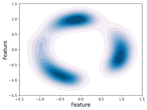
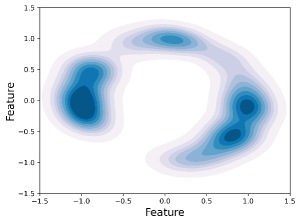
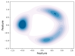
How to explore the correlation among multiple graphs is a critical problem in multi-view learning. Lyu et al (Lyu et al. 2022) theoretically illustrate that the correlation-based objective functions are effective in extracting shared and private information in multi-view data under some assumptions. Among them, Barlow Twins (Zbontar et al. 2021) is particularly popular. It consists of two parts: the invariance term maximizes the correlation between the same feature across different views, while the redundancy term decorrelates different features across various views. The feature decorrelation operation not only exploits the correlation of multiple views but also effectively alleviates the problem of representation collapse in self-supervised learning. This idea has been applied to graph clustering, such as MVGC (Xia et al. 2022) and MGDCR (Mo et al. 2023). However, existing methods simply use Barlow Twins, without any special operations catering to multi-relational graphs. Consequently, they still suffer from collapse. To show this, we visualize the feature distributions of several representative methods in ACM data: contrastive learning-based method MGCCN (Liu et al. 2022b), Barlow Twins-based method MGDCR (Mo et al. 2023), and our proposed method Barlow Twins Guided Filter (BTGF). Comparing Figs. 1(a) and 1(b), we can observe the advantage of Barlow Twins. From Figs. 1(b) and 1(c), a more evident enhancement in BTGF can be found.

In this work, we reveal that an input with a negative semi-definite inner product will lead to a lower bound for Barlow Twins loss, while an input with a positive semi-definite inner product has an upper bound. To minimize Barlow Twins loss as much as possible, we employ a graph filter to make the inner product positive semi-definite. Therefore, our filter upper bounds Barlow Twins, which means that the loss will never be too large to dominate other terms.

(a) MGCCN

(b) MGDCR

(c) BTGF

Figure 1: Visualization of representation distributions utilizing Gaussian Kernel Density Estimation (KDE) (Botev, Grotowski, and Kroese 2010) on ACM. Representations are mapped onto a two-dimensional normalized vector through t-SNE. A darker color indicates a higher concentration of points within the area. A better collapse mitigation method makes the feature distributions more uniform.

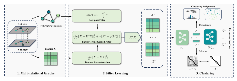
The overall architecture for multi-relational clustering is displayed in Fig. 2. The learned graph filter aggregates information for each node from its neighbors, resulting in smooth representations. They serve as input to an encoder, which maps them into a clustering-favorable space. Subsequently, they are reconstructed by a decoder. After training, clustering results are obtained using the output of the encoder.

The main contributions of this paper can be summarized in three aspects:

• We conduct a theoretical analysis to examine how the input affects the optimization of Barlow Twins. An input with a negative semi-definite inner product provides a lower bound for Barlow Twins loss, while an input with a positive semi-definite inner product yields an upper bound.

• A graph filter that facilitates Barlow Twins optimization is designed. This filter ensures that the inner product of the encoder input is positive semi-definite, which enables Barlow Twins to have an upper bound and surpass the lower bound, leading to improved performance.

• A simple yet effective clustering architecture is developed. Experimental results on four multi-relational graph datasets demonstrate the superiority of BTGF, even when the network just employs a linear layer.

Related Work

In recent years, numerous multi-view graph clustering methods have been proposed. Shallow methods MvAGC (Lin and Kang 2021) and MCGC (Pan and Kang 2021) employ a low-pass filter to embed relation information into attributes, and have achieved impressive results. Nevertheless, they just use a simple weight to differentiate various views and don’t explicitly consider the correlations among different views.

Distinct from the shallow methods described above, deep methods attempt to learn good representations via designed neural networks. O2MAC (Fan et al. 2020) and MAGCN (Cheng et al. 2021) cluster multi-relational graphs using GCN. CMGEC (Wang et al. 2021b) applies mutual information maximization to capture complementary and consistent information of each view. HAN (Wang et al. 2019) and HDMI (Jing, Park, and Tong 2021) apply the attention mechanism to fuse different relations. Due to the importance of structure in different views (Fang et al. 2022), MGCCN (Liu et al. 2022a) introduces a contrastive learning mechanism to capture consistent information between diverse views. However, these methods could be subject to representation collapse.

Two popular solutions to mitigate representation collapse are asymmetric model architecture, e.g., MoCo (He et al. 2020), BYOL (Grill et al. 2020), SimSiam (Chen and He 2021), and appropriate objective function, e.g., SimCLR (Chen et al. 2020), Barlow Twins (Zbontar et al. 2021). BT introduces a novel cross-correlation objective function for feature decorrelation. Owing to its concise implementation, without negative sample generation and asymmetric networks, it has gained popularity in self-supervised learning (Zhang et al. 2021, 2022). Graph Barlow Twins (Bielak, Kajdanowicz, and Chawla 2022) optimizes the embeddings of two distorted views of a graph. Clustering methods are also prone to collapse, e.g., empty clusters in K-means. DCRN (Liu et al. 2022b) extends the idea of Barlow Twins into deep clustering and designs a dual correlation reduction network to address representation collapse. However, it is a single-view model and cannot handle multi-relational graphs. DGCN (Pan and Kang 2023a) uses similar correlation reduction item to alleviate collapse. MVGC (Xia et al. 2022) and MGDCR (Mo et al. 2023) directly apply Barlow Twins to multi-relational graphs. However, they suffer insufficient optimization. In this paper, we theoretically analyze the conditions for the existence of lower and upper bounds for Barlow Twins loss and design a new filter based on it.

Figure 2: The proposed framework for multi-relational clustering.

Methodology

Notation

Define the multi-relational graph as $G=\left\{\mathcal{V},E_{1},\ldots,E_{V},X\right\}$, where $\mathcal{V}$ represents the sets of $n$ nodes, $e_{ij}\in E_{v}$ denotes the relationship between node $i$ and node $j$ in the $v$-th view. ${V}\geq 1$ is the number of relational graphs. $X=\left\{x_{1},\ldots,x_{n}\right\}^{\top}\in{R}^{n\times f}$ is the attribute matrix, $f$ is the dimension of features. The adjacency matrix $\widetilde{A}^{v}$ characterizes the initial graph structure of the $v$-th view. $D^{v}$ represents the degree matrices. The normalized adjacency matrix is $A^{v}=\left(D^{v}\right)^{-\frac{1}{2}}\left(\widetilde{A}^{v}+I\right)\left(D^{v}\right)^{-\frac{1}{2}}$ and the corresponding graph Laplacian is $L^{v}=I-A^{v}$. And $c$ represents the number of node classes.

Barlow Twins Guided Filter

To inject the topology structure into features, graph filtering is performed as:

$$\widetilde{X}^{v}=g(L^{v})X,$$ (1)

where $g(L^{v})$ is the $v$-th view’s graph filter. Then, we represent the encoder as a multi-layer dimensional transformation $W\in R^{f\times d}$, where $d$ is the output dimension of the embedding $Z$. We can express $Z^{v}$ as:

$$Z^{v}=g(L^{v})XW.$$ (2)

Specifically, we aim to learn a single encoder $h:R^{n\times f}\to R^{n\times d}$ for different views, i.e., the encoders $Z^{v}=h(\widetilde{X}^{v})$ share the same parameters. Afterward, we compute Barlow Twins (BT) as follows:

$$\mathcal{L}^{v_{1},v_{2}}_{BT} =\sum_{i=1}^{d}\left(M^{v_{1},v_{2}}_{ii}-1\right)^{2}+\lambda\sum_{i=1}^{d}\sum_{j\neq i}^{d}(M^{v_{1},v_{2}}_{ij})^{2},$$ (3)

$$M^{v_{1},v_{2}}_{ij}=\frac{{Z^{v_{1}}_{:i}}^{\top}Z^{v_{2}}_{:j}}{\left\|Z^{v_{1}}_{:i}\right\|\cdot\left\|Z^{v_{2}}_{:j}\right\|}=(\hat{Z}^{v_{1}}_{:i})^{\top}\hat{Z}^{v_{2}}_{:j},$$

where $\hat{Z}^{v}$ is the column-normalized form of $Z^{v}$, i.e., $\hat{Z}^{v}=Z^{v}(\Lambda^{v})^{-1}$, $\Lambda^{v}$ is a diagonal matrix with positive elements $\left\|Z^{v}_{:i}\right\|$. $\lambda$ is a trade-off parameter that balances the invariance term and redundancy reduction term, which is fixed to 0.0051 (Zbontar et al. 2021).

To enhance the effectiveness of BT loss on multi-relational graphs, we first provide some theoretical analysis. We find that the convergence of BT is influenced by the inner product between $\widetilde{X}^{v_{1}}$ and $\widetilde{X}^{v_{2}}$.

Proposition 1.

Barlow Twins has an explicit lower bound $\sum_{i=1}^{d}(\frac{\Lambda^{v_{1}}_{ii}\Lambda^{v_{2}}_{ii}}{max(\Lambda^{v_{1}}_{ii})max(\Lambda^{v_{2}}_{ii})})^{2}$, if $(g(L^{v_{1}})X)^{\top}g(L^{v_{2}})X$ is negative semi-definite.

Proof.

Denote $(g(L^{v_{1}})X)^{\top}g(L^{v_{2}})X$ as $H^{v_{1},v_{2}}\in R^{f\times f}.$

$$M^{v_{1},v_{2}} =(\Lambda^{v_{1}})^{-1}{W}^{\top}(g(L^{v_{1}})X)^{\top}g(L^{v_{2}})XW(\Lambda^{v_{2}})^{-1}$$ (4)

$$=(\Lambda^{v_{1}})^{-1}{W}^{\top}H^{v_{1},v_{2}}W(\Lambda^{v_{2}})^{-1},$$

$$\mathcal{L}^{v_{1},v_{2}}_{BT} =\sum_{i=1}^{d}\left(M^{v_{1},v_{2}}_{ii}-1\right)^{2}+\lambda\sum_{i=1}^{d}\sum_{j\neq i}^{d}(M^{v_{1},v_{2}}_{ij})^{2}$$

$$\underset{(1.a)}{>}\sum_{i=1}^{d}\left(M^{v_{1},v_{2}}_{ii}-1\right)^{2}$$

$$=\sum_{i=1}^{d}(\frac{1}{\Lambda^{v_{1}}_{ii}\Lambda^{v_{2}}_{ii}}{W}_{:i}^{\top}H^{v_{1},v_{2}}{W}_{:i}-1)^{2}$$

$$\geq\sum_{i=1}^{d}(\frac{{W}_{:i}^{\top}H^{v_{1},v_{2}}{W}_{:i}-\Lambda^{v_{1}}_{ii}\Lambda^{v_{2}}_{ii}}{max(\Lambda^{v_{1}}_{ii})max(\Lambda^{v_{2}}_{ii})})^{2}$$

$$\underset{(1.b)}{\geq}\sum_{i=1}^{d}(\frac{\Lambda^{v_{1}}_{ii}\Lambda^{v_{2}}_{ii}}{max(\Lambda^{v_{1}}_{ii})max(\Lambda^{v_{2}}_{ii})})^{2},$$

where (1.a): $\lambda>0$ and (1.b): Since $H^{v_{1},v_{2}}$ is negative semi-definite, we have ${W}_{:i}^{\top}H^{v_{1},v_{2}}{W}_{:i}\leq 0$, which implies $({W}_{:i}^{\top}H^{v_{1},v_{2}}{W}_{:i}-\Lambda^{v_{1}}_{ii}\Lambda^{v_{2}}_{ii})^{2}\geq(\Lambda^{v_{1}}_{ii}\Lambda^{v_{2}}_{ii})^{2}.$ ∎

The optimization objective of BT is to make the diagonal elements converge to 1 and the off-diagonal elements converge to zero, thus driving the BT value close to zero. However, having a constant positive lower bound in Proposition. 1 undermines the capability of BT to effectively explore multi-view correlations and alleviate representation collapse. Additionally, clustering models often involve several loss terms for multi-objective optimization. Consequently, BT could be influenced by other losses during the training process, which makes it impossible to reach zero. To address this problem, we attempt to impose an upper bound on BT.

Proposition 2.

If $H^{v_{1},v_{2}}$ is a positive semi-definite matrix, Barlow Twins will be upper bound by $d+\lambda\sum_{i=1}^{d}\sum_{j\neq i}^{d}(M^{v_{1},v_{2}}_{ij})^{2}$.

Proof.

$$\mathcal{L}^{v_{1},v_{2}}_{BT} =\sum_{i=1}^{d}(\frac{1}{\Lambda^{v_{1}}_{ii}\Lambda^{v_{2}}_{ii}}{W}_{:i}^{\top}H^{v_{1},v_{2}}{W}_{:i}-1)^{2}$$ (5)

$$+\lambda\sum_{i=1}^{d}\sum_{j\neq i}^{d}(M^{v_{1},v_{2}}_{ij})^{2}$$

$$\underset{(2.a)}{\leq}d+\lambda\sum_{i=1}^{d}\sum_{j\neq i}^{d}(M^{v_{1},v_{2}}_{ij})^{2},$$

where (2.a): $M^{v_{1},v_{2}}_{ii}$ is the cosine similarity of $Z^{v_{1}}_{:i}$ and $Z^{v_{2}}_{:i}$, so $M^{v_{1},v_{2}}_{ii}\in[-1,1]$. If $H$ is positive semi-definite, we have $M^{v_{1},v_{2}}_{ii}=\frac{1}{\Lambda^{v_{1}}_{ii}\Lambda^{v_{2}}_{ii}}{W}_{:i}^{\top}H^{v_{1},v_{2}}{W}_{:i}\geq 0$, i.e., $M^{v_{1},v_{2}}_{ii}\in[0,1]$. Therefore, the first term is bounded by $d$. ∎

The positive semi-definite property in the Proposition. 2 prevents BT from having the lower bound in Proposition. 1. More importantly, this upper bound constrains BT loss to a small range. Consequently, to improve the performance of BT in real applications, we design a filter that ensures $H^{v_{1},v_{2}}$ be positive semi-definite. A simple way is to let $(g(L^{v_{1}})X)^{\top}g(L^{v_{2}})X\approx X^{\top}X$, which is positive semi-definite due to the nature of the inner product of matrices. For notation simplicity, we use $K\in{\cal{R}}^{n\times n}$ to represent the filter $g(\cdot)$. The filter can be approximately obtained by solving the following problem:

$$\min_{K}\left\|X-KX\right\|_{F}^{2},$$ (6)

where $\|\cdot\|_{F}$ denotes the Frobenius norm. Eq. 6 could produce a trivial solution and it neglects the rich topology information in graphs. Hence, we design a regularizer to preserve the most important low-frequency information. Considering the variation in each graph, we learn a filter for each view.

$$\min_{K^{v}}\left\|{X}-K^{v}{X}\right\|_{F}^{2}+\gamma\|K^{v}-\varphi(L^{v})\|_{F}^{2},$$ (7)

where $\gamma>0$ is trade-off parameter and $\varphi(L^{v})$ is a typical low-pass filter (Zhang et al. 2019):

$$\varphi(L^{v})=(I-\frac{L^{v}}{2})^{k},$$ (8)

where $k$ is the filter order. Eq. 7 can be easily solved by setting its first-order derivative w.r.t. $K^{v}$ to zero, which yields,

$$K^{v}=\left(X{X}^{\top}+\gamma I\right)^{-1}\left(\gamma\varphi(L^{v})+X{X}^{\top}\right).$$ (9)

However, the $\mathcal{O}\left(n^{3}\right)$ computational complexity of the inverse operation is expensive. This problem can be alleviated by using the Woodbury matrix identity (Higham 2002). Then, the graph filter $K^{v}$ can be reformulated as follows:

$$K^{v}= [\frac{1}{\gamma}I-\frac{1}{\gamma^{2}}X(I+\frac{1}{\gamma}{X}^{\top}{X})^{-1}{X}^{\top}]\left(\gamma\varphi(L^{v})+{X}{X}^{\top}\right)$$ (10)

$$= \frac{X{X}^{\top}}{\gamma}-\frac{X(I+\frac{1}{\gamma}{X}^{\top}{X})^{-1}{X}^{\top}\left(\gamma\varphi(L^{v})+X{X}^{\top}\right)}{\gamma^{2}}$$

$$+\varphi(L^{v}).$$

The complexity is reduced from $\mathcal{O}\left(n^{3}\right)$ to $\mathcal{O}\left(n^{2}f\right)$ when $n>f$. It can be seen from Eq. 10 that the filter is essentially a feature-based modification to the conventional filter, which is solely based on graph structure. Different from existing works (Pan and Kang 2021; Lin and Kang 2021), the filters are not independent for each graph but correlated by feature, thus they can capture the correlations between views to some extent.

Multi-relational Graph Clustering

The multi-relational graph is first processed by the filter to obtain $\widetilde{X}^{v}$:

$$\widetilde{X}^{v}=K^{v}X.$$ (11)

The smoothed features $\widetilde{X}^{v}$ integrate view-specific topology with the node attributes. We then feed $\widetilde{X}$ into a network that consists of linear layers. Specifically, the encoder and decoder for each view share the same parameters, so the entire network can be considered as one auto-encoder.

The encoder maps $\widetilde{X}^{v}$ into feature subspace to obtain embedding $Z^{v}$. The embeddings from different views are paired to compute Barlow Twins, and the resulting values are averaged. We denote the result as a feature decorrelation loss:

$$\mathcal{L}_{FD}=\frac{1}{\tbinom{V}{2}}\sum^{V}_{v_{1}\not=v_{2}}\sum^{V}_{v_{2}=1}\mathcal{L}^{v_{1},v_{2}}_{BT}.$$ (12)

We use target distribution and soft cluster assignment probabilities distribution to enhance clustering quality (Tu et al. 2021). All embeddings are concatenated into $Z=[Z^{1},Z^{2},...,Z^{V}]\in R^{n\times Vd}$ as the input to this self-supervised clustering module. The soft assignment distribution $Q$ can be formulated as:

$$q_{ij}=\frac{{\left(1+\left\|z_{i}-\sigma_{j}\right\|^{2}\right)}^{-1}}{\sum_{j^{\prime}}\left(1+\left\|z_{i}-\sigma_{j^{\prime}}\right\|^{2}\right)^{-1}},$$ (13)

where $q_{ij}$ is measured by Student’s $t$-distribution to indicate the similarity between node $i$’s embedding $z_{i}$ and clustering center $\sigma_{j}$ that is initialized by the centers resulting from the $k$-means implemented on $Z$. The target distribution $P$ is computed as:

$$p_{ij}=\frac{q_{ij}^{2}/\sum_{i}q_{ij}}{\sum_{j^{\prime}}\left(q_{ij^{\prime}}^{2}/\sum_{i}q_{ij^{\prime}}\right)}.$$ (14)

We then minimize the KL divergence between the $Q$ and $P$ distributions to encourage the data representation to align with cluster centers and enhance cluster cohesion (Kullback and Leibler 1951):

$$\mathcal{L}_{CLU}=KL(P\|Q)=\sum_{i}\sum_{u}p_{iu}\log\frac{p_{iu}}{q_{iu}}.$$ (15)

Afterward, the decoder is utilized to obtain reconstructed features:

$$\bar{X}^{v}=Z^{v}W_{de},$$ (16)

where $W_{de}\in R^{d\times f}$. It is worth noting that the features of certain “easy samples” only exhibit tiny changes during reconstruction, suggesting that these nodes provide little informative input for our network. The Scaled Cosine Error (SCE) (Hou et al. 2022) is adopted as the reconstruction objective function in our model for down-weighting the contribution of those easy samples:

$$\mathcal{L}^{v}_{SCE}=\sum_{i=1}^{n}\left(1-\frac{{(\widetilde{X}^{v}_{i})^{\top}\bar{X}^{v}_{i}}}{{\|\widetilde{X}^{v}_{i}\|\cdot\|\bar{X}^{v}_{i}\|}}\right)^{2}$$ (17)

Same as Barlow Twins, $\mathcal{L}_{SCE}$ needs to be summed and averaged:

$$\mathcal{L}_{MSCE}=\frac{1}{V}\sum^{V}_{v=1}\mathcal{L}^{v}_{SCE}.$$ (18)

By combining $\mathcal{L}_{FD}$, $\mathcal{L}_{MSCE}$, and $\mathcal{L}_{CLU}$, the overall objective function of BTGF can be computed as:

$$\mathcal{L}=\mathcal{L}_{MSCE}+\mathcal{L}_{FD}+\mathcal{L}_{CLU}.$$ (19)

We minimize the above objective function to optimize our auto-encoder and achieve the cluster label $y_{i}$ for node $i$ by:

$$y_{i}=\underset{j}{\operatorname{argmax}}\hskip 1.13809ptq_{ij}.$$ (20)

Experiment

Table 1: The statistics of datasets.

Datasets	Nodes	Relation Types	Edges	Attributes	Classes
ACM	3,025	Paper-Author-Paper Paper-Subject-Paper	29,281 2,210,761	1, 830	3
AMiner	6,564	Paper-Author-Paper Paper-Reference-Paper	15,412 123,260	6,564	4
DBLP	7, 907	Paper-Paper-Paper Paper-Author-paper	90,145 144,783	2, 000	4
Amazon	7, 621	Item-AlsoView-Item Item-AlsoBought-Item Item-BoughtTogether-Item	266,237 1,104,257 16,305	2, 000	4

Table 2: Node clustering results.

Dataset	ACM				DBLP				Amazon				AMiner
Metric	ACC	F1	NMI	ARI	ACC	F1	NMI	ARI	ACC	F1	NMI	ARI	ACC	F1	NMI	ARI
HAN(2019)	0.8823	0.8844	0.5881	0.5933	0.7651	0.6309	0.4866	0.4635	0.4355	0.4246	0.1120	0.0362	0.7119	0.5340	0.2020	0.1260
O2MAC(2020)	0.9042	0.9053	0.6923	0.7394	0.7267	0.7320	0.4066	0.4036	0.4428	0.4424	0.1344	0.0898	0.4939	0.3202	0.0857	0.0552
MvAGC(2021)	0.8975	0.8986	0.6735	0.7212	0.7221	0.7332	0.4191	0.4049	0.5188	0.5072	0.2322	0.1141	0.5472	0.1781	0.0452	0.0003
HDMI(2021)	0.8740	0.8720	0.6450	0.6740	0.8010	0.7898	0.5820	0.5356	0.5251	0.5448	0.3702	0.2735	0.4032	0.3023	0.1349	0.0314
MCGC(2021)	0.9147	0.9155	0.7126	0.7627	0.7850	0.7359	0.5510	0.4439	0.4683	0.4804	0.2149	0.1056	0.4165	0.3982	0.2254	0.1608
MGCCN(2022)	0.9167	0.8472	0.7095	0.7688	0.8301	0.7336	0.6156	0.5876	0.5309	0.4572	0.1931	0.1860	0.6039	0.5311	0.2039	0.2883
MGDCR(2023)	0.9190	0.8678	0.7210	0.6496	0.8070	0.8048	0.6140	0.5259	0.3489	0.2039	0.0318	0.0055	0.5150	0.2533	0.0265	0.0300
BTGF	0.9322	0.9331	0.758	0.8085	0.8309	0.8384	0.6242	0.5969	0.6603	0.6612	0.3853	0.2829	0.7308	0.5408	0.3603	0.5233

Datasets and Metrics

To show the effectiveness of BTGF, we evaluate our method on four multi-relational graphs. ACM and DBLP (Fan et al. 2020) are citation graph networks. Amazon (He and McAuley 2016) is a review graph network. AMiner (Wang et al. 2021a) is an academic graph network. The statistical information of them is summarized in Table 1. We adopt four popular clustering metrics, including ACCuracy (ACC), Normalized Mutual Information (NMI), F1 score, and Adjusted Rand Index (ARI). A higher value of them indicates a better performance.

Experimental Setup

Parameter Setting

The experiments are implemented in the PyTorch platform using an Intel(R) Core(TM) i9-12900k CPU, and GeForce GTX 3090 24G GPU. Our auto-encoder is trained by Adam optimizer (Kingma and Ba 2015) for 400 epochs. For simplicity, both our encoder and decoder only have one linear layer, denoted as $W\in R^{f\times d}$, $W_{de}\in R^{d\times f}$ respectively, where $d=10$. The learning rate and weight decay of the optimizer are set to $1e^{-2}$ and $1e^{-3}$, respectively. The filter’s parameters $k$ and $\gamma$ is tuned in $[1,2,3,4,5]$ and $[0.1,1,10,100,1000]$, respectively.

Comparison Methods

We compare BTGF with multi-view methods: HAN (Wang et al. 2019) and HDMI (Jing, Park, and Tong 2021), which use the attention mechanism; O2MAC (Fan et al. 2020) clusters multi-relational data by selecting an informative graph. We also compare BTGF with contrastive learning methods, such as MCGC (Pan and Kang 2021) and MGCCN (Liu et al. 2022a). MvAGC (Lin and Kang 2021) and MGDCR (Mo et al. 2023) are also compared. Particularly, MvAGC and MCGC both employ graph filters to preprocess the attribute. MGDCR utilizes Barlow Twins as an objective function for multi-relational clustering. For an unbiased comparison, we copy part of the results from MCGC.

Clustering Results

The clustering results are reported in Table 2. From it, we have the following observations:

• The advantages of BTGF are clear when compared to deep multi-view clustering methods: HAN, HDMI, O2MAC, and MGCCN. With respect to the most recent MGCCN, our method improves ACC, F1, NMI, ARI by 11%, 16%, 45%, 34% on average, respectively. Note that MGCCN uses a contrastive learning mechanism to fuse representations of different views. As shown in Fig. 1, our superiority stems from the incorporation of Barlow Twins, which significantly enhances the integration of information from different graphs.

• In comparison to shallow MvAGC and MCGC methods, our approach greatly boosts clustering performance. Both MvAGC and MCGC employ a low-pass filter on each graph to smooth the attributes, which fails to consider the correlation between different views. This is exactly the issue that BTGF aims to tackle.

• BTGF outperforms Barlow Twins-based method MGDCR. In particular, the improvement on Amazon and AMiner is significant. This could be caused by the large number of hyperparameters introduced in computing the pairwise loss in MGDCR, which are hard to find the most appropriate values.

In summary, BTGF consistently outperforms all compared methods in terms of four metrics over all datasets. The stable results obtained with such a simple network demonstrate the validity of our filter and the clustering architecture. They could be further improved if a more complex auto-encoder architecture with deep artifices such as activation functions or dropout is applied.

Table 3: Clustering performance of variants of BTGF.

Datasets		ACM	DBLP	Amazon	AMiner
ACC	BTGF	0.9322	0.8309	0.6603	0.7308
	w/o $\mathcal{L}_{FD}$	0.9121	0.8212	0.5885	0.6817
	w/o $\mathcal{L}_{MSCE}$	0.9296	0.8041	0.5149	0.5506
F1	BTGF	0.9331	0.8384	0.6612	0.5308
	w/o $\mathcal{L}_{FD}$	0.9130	0.8273	0.5272	0.4688
	w/o $\mathcal{L}_{MSCE}$	0.9305	0.8080	0.4564	0.3209
NMI	BTGF	0.758	0.6242	0.3853	0.3603
	w/o $\mathcal{L}_{FD}$	0.6988	0.5900	0.3695	0.3540
	w/o $\mathcal{L}_{MSCE}$	0.7525	0.5760	0.2223	0.0612
ARI	BTGF	0.8085	0.5969	0.2829	0.5233
	w/o $\mathcal{L}_{FD}$	0.7553	0.5788	0.2590	0.5017
	w/o $\mathcal{L}_{MSCE}$	0.8019	0.5501	0.1640	0.1054

Ablation Study

The Effect of Different Loss Terms

To validate the effectiveness of different components in our model, we compare the performance of BTGF with its two variants:

• Employing BTGF without $\mathcal{L}_{FD}$ to show the importance of utilizing feature decorrelation.

• Employing BTGF without $\mathcal{L}_{MSCE}$ to observe the impact of the decoder and feature reconstruction. It means training an encoder with $\mathcal{L}_{FD}+\mathcal{L}_{CLU}$ and no decoder.

Based on Table 3, we can draw the following conclusions. Firstly, the results of BTGF are better than all variants, which indicates the validity of each term. Second, the Barlow Twins plays a crucial role in fusing different views. Especially for Amazon with three relation types, the impact of the correlation regularizer $\mathcal{L}_{FD}$ is huge. In addition, the feature reconstruction loss used to down-weight easy samples’ contribution is proved to be helpful in improving the clustering performance.

(a) ACM

(b) DBLP

(c) Amazon

(d) AMiner

Figure 3: Verification of $\mathcal{L}_{FD}$ surpassing the lower boundary as well as having an upper boundary.

(a) ACM

(b) DBLP

(c) Amazon

(d) AMiner

Figure 4: The evolution of feature decorrelation loss $\mathcal{L}_{FD}$ when using different filters.

Table 4: Clustering accuracy with different filters.

Datasets	ACM	DBLP	Amazon	AMiner
BTGF	0.9322	0.8309	0.6603	0.7308
w/ mix-pass filter	0.9250	0.8148	0.6462	0.5716
w/ low-pass filter	0.9088	0.8195	0.6184	0.7116
w/o filter	0.8707	0.7166	0.6004	0.3326

(a) ACM

(b) DBLP

(c) Amazon

(d) AMiner

Figure 5: The influence of $k$ and $\gamma$ on four datasets (metric: ACC).

The Effect of Graph Filter

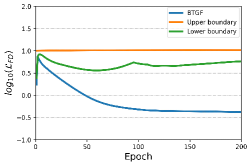
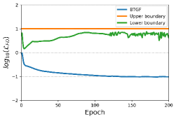
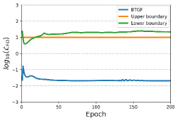
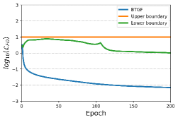
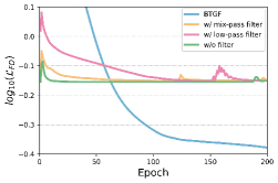
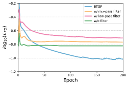
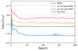
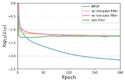
To illustrate the superiority of our filter, we plot the feature decorrelation loss $\mathcal{L}_{FD}$ with respect to the training epochs and examine three variants of BTGF:

• with low-pass filter $K=(I-\frac{L}{2})^{2}$ instead of Eq. 10;

• with mix-pass filter $K=(I-\frac{L}{2})^{2}+(\frac{L}{2})^{2}$ instead of Eq. 10;

• without using graph filter as preprocessing.

There are three findings:

Obs 1: As shown in Fig. 3, our $\mathcal{L}_{FD}$ loss has the smallest value. According to our Propositions, the positive semi-definite constraint on the feature can restrict the upper boundary of $\mathcal{L}_{FD}$ and break through the lower boundary, reaching a lower value. The evolution of $\mathcal{L}_{FD}$ is in line with our expectations. Note that the upper and lower bounds depend on the output of the encoder, exhibiting variation among different methods and datasets, and evolving throughout the training process. It is interesting to see that our upper bound is even smaller than the lower bound on Amazon, suggesting that we can find a better solution than an input with negative semi-definite inner product. This could explain our dramatic improvement on Amazon.

Obs 2: As shown in Fig. 4, our $\mathcal{L}_{FD}$ converges to smaller values compared to other filters. This indicates that our filter is more effective, which in turn improves the performance of downstream tasks. This is demonstrated in Table 4.

Obs 3: The absence of filters produces the worst results, which validates the importance of fusing the topology structure and attribute information. Moreover, the low-pass and mix-pass filters generate inferior performance due to their neglect of the correlation between the multi-relational graphs.

Parameter Analysis

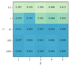
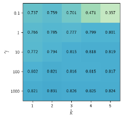
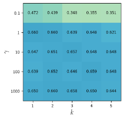
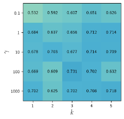
This section analyzes the sensitivity of parameters in BTGF across four datasets. There are only two parameters, $k$ and $\gamma$, in the graph filter. Their influence on precision is demonstrated in Fig. 5. Overall, BTGF produces reasonable performance. On the one hand, a smaller value of $\gamma$ prevents the filter from effectively utilizing the topological information of multi-relational graphs, leading to impaired clusters. On the other hand, an excessively large $\gamma$ could cause the filter to completely converge to a low-pass filter, which in turn neglects the constraint on the input. In addition, BTGF performs well for a small range of $k$, which is also convenient for practical application.

Conclusion

In this work, we find that the graph filter can impact the performance of Barlow Twins by analyzing the conditions for the existence of lower and upper bounds of Barlow Twins loss. We prove that an input with a positive semi-definite inner product yields an upper bound, which is potentially beneficial when applying Barlow Twins. Based on this finding, we design a novel graph filter that captures the correlations between multi-relational graphs. Afterward, a simple architecture, which incorporates multi-view correlation, feature decorrelation, and graph filtering, is developed for multi-relational clustering. Comprehensive experiments on four benchmark datasets demonstrate the effectiveness of our approach. The filter design guided by loss warrants further investigation in other scenarios, e.g., GNN.

References

- Bielak, Kajdanowicz, and Chawla (2022) Bielak, P.; Kajdanowicz, T.; and Chawla, N. V. 2022. Graph barlow twins: A self-supervised representation learning framework for graphs. Knowledge-Based Systems, 256: 109631.
- Botev, Grotowski, and Kroese (2010) Botev, Z.; Grotowski, J.; and Kroese, D. 2010. Kernel density estimation via diffusion. Annals of Statistics, 38(5): 2916–2957.
- Chen et al. (2020) Chen, T.; Kornblith, S.; Norouzi, M.; and Hinton, G. 2020. A simple framework for contrastive learning of visual representations. In International conference on machine learning, 1597–1607. PMLR.
- Chen and He (2021) Chen, X.; and He, K. 2021. Exploring simple siamese representation learning. In Proceedings of the IEEE/CVF conference on computer vision and pattern recognition, 15750–15758.
- Cheng et al. (2021) Cheng, J.; Wang, Q.; Tao, Z.; Xie, D.; and Gao, Q. 2021. Multi-view attribute graph convolution networks for clustering. In Proceedings of the twenty-ninth international conference on international joint conferences on artificial intelligence, 2973–2979.
- Fan et al. (2020) Fan, S.; Wang, X.; Shi, C.; Lu, E.; Lin, K.; and Wang, B. 2020. One2multi graph autoencoder for multi-view graph clustering. In proceedings of the web conference 2020, 3070–3076.
- Fang et al. (2022) Fang, R.; Wen, L.; Kang, Z.; and Liu, J. 2022. Structure-preserving graph representation learning. In 2022 IEEE International Conference on Data Mining (ICDM), 927–932. IEEE.
- Grill et al. (2020) Grill, J.-B.; Strub, F.; Altché, F.; Tallec, C.; Richemond, P.; Buchatskaya, E.; Doersch, C.; Avila Pires, B.; Guo, Z.; Gheshlaghi Azar, M.; et al. 2020. Bootstrap your own latent-a new approach to self-supervised learning. Advances in neural information processing systems, 33: 21271–21284.
- He et al. (2020) He, K.; Fan, H.; Wu, Y.; Xie, S.; and Girshick, R. 2020. Momentum contrast for unsupervised visual representation learning. In Proceedings of the IEEE/CVF conference on computer vision and pattern recognition, 9729–9738.
- He and McAuley (2016) He, R.; and McAuley, J. 2016. Ups and downs: Modeling the visual evolution of fashion trends with one-class collaborative filtering. In proceedings of the 25th international conference on world wide web, 507–517.
- Higham (2002) Higham, N. J. 2002. Accuracy and stability of numerical algorithms. SIAM.
- Hou et al. (2022) Hou, Z.; Liu, X.; Cen, Y.; Dong, Y.; Yang, H.; Wang, C.; and Tang, J. 2022. Graphmae: Self-supervised masked graph autoencoders. In Proceedings of the 28th ACM SIGKDD Conference on Knowledge Discovery and Data Mining, 594–604.
- Jing, Park, and Tong (2021) Jing, B.; Park, C.; and Tong, H. 2021. Hdmi: High-order deep multiplex infomax. In Proceedings of the Web Conference 2021, 2414–2424.
- Kingma and Ba (2015) Kingma, D. P.; and Ba, J. 2015. Adam: A Method for Stochastic Optimization. In Proceedings of the International Conference on Learning Representations (ICLR) 2015.
- Kullback and Leibler (1951) Kullback, S.; and Leibler, R. A. 1951. On information and sufficiency. The annals of mathematical statistics, 22(1): 79–86.
- Lin and Kang (2021) Lin, Z.; and Kang, Z. 2021. Graph Filter-based Multi-view Attributed Graph Clustering. In IJCAI, 2723–2729.
- Lin et al. (2023) Lin, Z.; Kang, Z.; Zhang, L.; and Tian, L. 2023. Multi-View Attributed Graph Clustering. IEEE Transactions on Knowledge & Data Engineering, 35(02): 1872–1880.
- Liu et al. (2022a) Liu, L.; Kang, Z.; Ruan, J.; and He, X. 2022a. Multilayer Graph Contrastive Clustering Network. Inf. Sci., 613(C): 256–267.
- Liu et al. (2022b) Liu, Y.; Tu, W.; Zhou, S.; Liu, X.; Song, L.; Yang, X.; and Zhu, E. 2022b. Deep graph clustering via dual correlation reduction. In Proceedings of the AAAI Conference on Artificial Intelligence, volume 36, 7603–7611.
- Lyu et al. (2022) Lyu, Q.; Fu, X.; Wang, W.; and Lu, S. 2022. Understanding latent correlation-based multiview learning and self-supervision: An identifiability perspective. In International Conference on Learning Representations.
- Mo et al. (2023) Mo, Y.; Chen, Y.; Lei, Y.; Peng, L.; Shi, X.; Yuan, C.; and Zhu, X. 2023. Multiplex Graph Representation Learning Via Dual Correlation Reduction. IEEE Transactions on Knowledge and Data Engineering.
- Nie et al. (2017) Nie, F.; Li, J.; Li, X.; et al. 2017. Self-weighted Multiview Clustering with Multiple Graphs. In IJCAI, 2564–2570.
- Pan and Kang (2021) Pan, E.; and Kang, Z. 2021. Multi-view contrastive graph clustering. Advances in neural information processing systems, 34: 2148–2159.
- Pan and Kang (2023a) Pan, E.; and Kang, Z. 2023a. Beyond Homophily: Reconstructing Structure for Graph-agnostic Clustering. In Proceedings of the 40th International Conference on Machine Learning, 26868–26877.
- Pan and Kang (2023b) Pan, E.; and Kang, Z. 2023b. High-order multi-view clustering for generic data. Information Fusion, 100: 101947.
- Qu et al. (2017) Qu, M.; Tang, J.; Shang, J.; Ren, X.; Zhang, M.; and Han, J. 2017. An attention-based collaboration framework for multi-view network representation learning. In Proceedings of the 2017 ACM on Conference on Information and Knowledge Management, 1767–1776.
- Tu et al. (2021) Tu, W.; Zhou, S.; Liu, X.; Guo, X.; Cai, Z.; Zhu, E.; and Cheng, J. 2021. Deep fusion clustering network. In Proceedings of the AAAI Conference on Artificial Intelligence, volume 35, 9978–9987.
- Wang et al. (2019) Wang, X.; Ji, H.; Shi, C.; Wang, B.; Ye, Y.; Cui, P.; and Yu, P. S. 2019. Heterogeneous Graph Attention Network. In The World Wide Web Conference, WWW ’19, 2022–2032.
- Wang et al. (2021a) Wang, X.; Liu, N.; Han, H.; and Shi, C. 2021a. Self-supervised heterogeneous graph neural network with co-contrastive learning. In Proceedings of the 27th ACM SIGKDD conference on knowledge discovery & data mining, 1726–1736.
- Wang et al. (2021b) Wang, Y.; Chang, D.; Fu, Z.; and Zhao, Y. 2021b. Consistent multiple graph embedding for multi-view clustering. IEEE Transactions on Multimedia.
- Xia et al. (2022) Xia, W.; Wang, S.; Yang, M.; Gao, Q.; Han, J.; and Gao, X. 2022. Multi-view graph embedding clustering network: Joint self-supervision and block diagonal representation. Neural Networks, 145: 1–9.
- Zbontar et al. (2021) Zbontar, J.; Jing, L.; Misra, I.; LeCun, Y.; and Deny, S. 2021. Barlow twins: Self-supervised learning via redundancy reduction. In International Conference on Machine Learning, 12310–12320. PMLR.
- Zhang et al. (2022) Zhang, S.; Qiu, L.; Zhu, F.; Yan, J.; Zhang, H.; Zhao, R.; Li, H.; and Yang, X. 2022. Align representations with base: A new approach to self-supervised learning. In Proceedings of the IEEE/CVF Conference on Computer Vision and Pattern Recognition, 16600–16609.
- Zhang et al. (2021) Zhang, S.; Zhu, F.; Yan, J.; Zhao, R.; and Yang, X. 2021. Zero-cl: Instance and feature decorrelation for negative-free symmetric contrastive learning. In International Conference on Learning Representations.
- Zhang et al. (2019) Zhang, X.; Liu, H.; Li, Q.; and Wu, X. M. 2019. Attributed graph clustering via adaptive graph convolution. In 28th International Joint Conference on Artificial Intelligence, IJCAI 2019.