Weighted least-squares approximation with determinantal point processes and generalized volume sampling

Abstract

We consider the problem of approximating a function from $L^{2}$ by an element of a given $m$-dimensional space $V_{m}$, associated with some feature map $\boldsymbol{\varphi}$, using evaluations of the function at random points $x_{1},\ldots,x_{n}$. After recalling some results on optimal weighted least-squares using independent and identically distributed points, we consider weighted least-squares using projection determinantal point processes (DPP) or volume sampling. These distributions introduce dependence between the points that promotes diversity in the selected features $\boldsymbol{\varphi}(x_{i})$. We first provide a generalized version of volume-rescaled sampling yielding quasi-optimality results in expectation with a number of samples $n=O(m\log(m))$, that means that the expected $L^{2}$ error is bounded by a constant times the best approximation error in $L^{2}$. Also, further assuming that the function is in some normed vector space $H$ continuously embedded in $L^{2}$, we further prove that the approximation is almost surely bounded by the best approximation error measured in the $H$-norm. This includes the cases of functions from $L^{\infty}$ or reproducing kernel Hilbert spaces. Finally, we present an alternative strategy consisting in using independent repetitions of projection DPP (or volume sampling), yielding similar error bounds as with i.i.d. or volume sampling, but in practice with a much lower number of samples. Numerical experiments illustrate the performance of the different strategies.

Weighted least-squares, Optimal sampling, Determinantal point process, Volume sampling.

1 Introduction

We consider the problem of approximating a function $f$ by an element of a given $m$-dimensional space $V_{m}$ using point evaluations of the function. The function is defined on a general Polish space $\mathcal{X}$ equipped with a probability measure $\mu$ and the error is assessed in the natural norm in $L^{2}_{\mu}(\mathcal{X})$ defined by

$$\|f\|^{2}=\int_{\mathcal{X}}|f(x)|^{2}d\mu(x).$$

The best approximation error that can be achieved by elements of $V_{m}$ is

$$\inf_{v\in V_{m}}\|f-g\|=\|f-P_{V_{m}}f\|$$

where $P_{V_{m}}f$ is the orthogonal projection of $f$ onto $V_{m}$. An approximation $\hat{f}_{m}$ can be obtained by a weighted least-squares projection of $f$ defined as the minimizer of

$$\min_{g\in V_{m}}\frac{1}{n}\sum_{i=1}^{n}w(x_{i})^{-1}(f(x_{i})-g(x_{i}))^{2}$$ (1)

where $w:\mathcal{X}\to\mathbb{R}$ is a strictly positive weight function and the $x_{1},\ldots,x_{n}$ are points in $\mathcal{X}$. The approximation $\hat{f}_{m}$ is said quasi-optimal if

$$\|f-\hat{f}_{m}\|\leq C\inf_{g\in V_{m}}\|f-g\|,$$

with a constant $C$ independent of $m.$ When using random points, it is said quasi-optimal in expectation whenever

$$\mathbb{E}(\|f-\hat{f}_{m}\|^{2})^{1/2}\leq C\inf_{g\in V_{m}}\|f-g\|.$$

A fundamental problem is to select points and weights that achieve quasi-optimality with a number of points as close as possible to the dimension $m$ of $V_{m}.$ The weighted least-squares approximation $\hat{f}_{m}$ defined by (1) is such that

$$\|f-\hat{f}_{m}\|_{n}=\min_{g\in V_{m}}\|f-g\|_{n}$$ (2)

where $\|\cdot\|_{n}$ is the empirical semi-norm defined by

$$\|f\|_{n}^{2}=\frac{1}{n}\sum_{i=1}^{n}w(x_{i})^{-1}f(x_{i})^{2}.$$ (3)

$\hat{f}_{m}$ is the orthogonal projection $\hat{P}_{V_{m}}f$ of $f$ onto $V_{m}$ with respect to the empirical semi-norm, and the quality of the approximation is related to how close $\|\cdot\|_{n}$ is from the norm $\|\cdot\|$.

We assume that we are given an orthonormal basis $\varphi_{1},\ldots,\varphi_{m}$ of $V_{m}$, and we let $\boldsymbol{\varphi}:\mathcal{X}\to\mathbb{R}^{m}$ be the associated feature map defined by $\boldsymbol{\varphi}(x)=(\varphi_{1}(x),\ldots,\varphi_{m}(x))^{T}$. Then for any $g$ in $V_{m}$, where $g(x)=\boldsymbol{\varphi}(x)^{T}\mathbf{a}$ for some $\mathbf{a}\in\mathbb{R}^{m}$, it holds $\|g\|^{2}=\|\mathbf{a}\|_{2}^{2}$ and $\|g\|_{n}^{2}=\mathbf{a}^{T}\mathbf{G}^{w}\mathbf{a},$ where $\mathbf{G}^{w}$ is the empirical Gram matrix

$$\mathbf{G}^{w}=\mathbf{G}^{w}(x_{1},\ldots,x_{m}):=\frac{1}{n}\sum_{i=1}^{n}w(x_{i})^{-1}\boldsymbol{\varphi}(x_{i})\boldsymbol{\varphi}(x_{i})^{T},$$ (4)

so that

$$\lambda_{min}(\mathbf{G}^{w})\|g\|^{2}\leq\|g\|_{n}^{2}\leq\lambda_{max}(\mathbf{G}^{w})\|g\|^{2},\quad\forall g\in V_{m}.$$ (5)

The quality of the projection is therefore related to how much the spectrum of $\mathbf{G}^{w}$ deviates from one. In particular, it holds

$$\|f-\hat{f}_{m}\|^{2}\leq\|f-P_{V_{m}}f\|^{2}+\lambda_{min}(\mathbf{G}^{w})^{-1}\|f-P_{V_{m}}f\|_{n}^{2},$$

A control of the minimal eigenvalue of $\mathbf{G}^{w}$ is therefore necessary to achieve quasi-optimality. A control of the highest eigenvalue of $\mathbf{G}^{w}$ is also needed for numerical stability reasons, so that quasi-optimality can be achieved in finite precision arithmetics. The choice of optimal points (and weights) is a classical problem of design of experiments [20]. A classical approach, called $E$-optimal design, consists in selecting points (and weights) that maximize $\lambda_{min}(\mathbf{G}^{w})$. Variants of this problem consist in maximizing the trace of the inverse of $\mathbf{G}^{w}$, which is called $A$-optimal design, or maximizing the determinant $\det(\mathbf{G}^{w})$, which is called $D$-optimal design. The latter is related to Fekete points for polynomial interpolation or more general kernel based interpolation [5, 14]. It is also related to maximum volume concept in linear algebra [12, 11]. However, these optimization problems are in general intractable.

The above mentioned approaches are deterministic. Here, we follow a probabilistic avenue, where the points $x_{1},\ldots,x_{n}$ are drawn from a suitable distribution allowing a control of the spectrum of the empirical Gram matrix. When the points $x_{i}$ are drawn from a distribution $\nu$ with density $w$ with respect to $\mu$, the empirical Gram matrix is an unbiased estimate of the identity. Provided the points are independent and identically distributed (i.i.d.), the empirical Gram matrix almost surely converges to the identity and matrix concentration inequalities allow to analyze how fast is this convergence. An optimization of the convergence rate over all possible distributions yields an optimal density $w_{m}(x)=\frac{1}{m}\|\boldsymbol{\varphi}(x)\|^{2}_{2}$, that is known as the inverse Christoffel function for polynomial spaces $V_{m}$ [6]. The measure $\nu_{m}=w_{m}\mu$ is also known as leverage score distribution in statistics and machine learning. Sampling from this distribution guarantees that the event $S_{\delta}=\{\lambda_{min}(\mathbf{G}^{w_{m}})\geq 1-\delta\}$ is satisfied with a controlled probability $1-\eta$ provided the number of samples $n=O(\delta^{-2}m\log(m\eta^{-1}))$, where the dependence in $m$ is known to be optimal for i.i.d. sampling [21]. A similar control in probability is obtained for the maximum eigenvalue, and $\lambda_{max}(\mathbf{G}^{w_{m}})\leq m$ even holds almost surely with the particular choice of weight function $w_{m}$. By drawing i.i.d. samples from $\nu_{m}$ and conditioning to the event $S_{\delta}$ (that can be achieved by a rejection sampling with controlled rejection probability), it holds $\mathbb{E}(\|\cdot\|_{n}^{2})\leq\beta\|\cdot\|^{2}$ for some constant $\beta$, and the resulting least-squares projection $\hat{f}_{m}$ is quasi-optimal in expectation. If we further assume that the target function $f$ is in a subspace $H$ continuously embedded in $L^{2}_{\mu}(\mathcal{X})$ and $L^{\infty}_{h^{-1/2}\mu}(\mathcal{X})$, with $h$ a probability density with respect to $\mu$, and if we choose for $\nu=w\mu$ a mixture of the optimal sampling distribution $\nu_{m}=w_{m}\mu$ and $h\mu$, we prove that quasi-optimality still holds in expectation and we also prove that $\|\cdot\|_{n}$ is almost surely bounded by $\|\cdot\|_{H}$ (up to a constant), which ensures that it holds almost surely

$$\|f-\hat{f}_{m}\|\leq C\inf_{g\in V_{m}}\|f-g\|_{H},$$ (6)

which we will call $H\to L^{2}_{\mu}$ quasi-optimality. Examples of such spaces $H$ are $L^{\infty}_{\mu}(\mathcal{X})$ (with density $h=1$), or reproducing kernel Hilbert spaces.

In practice, the number of i.i.d. samples $n$ needed for a stable projection may be large and far from the dimension $m$. In order to further reduce the sampling complexity, various subsampling approaches have been recently proposed. They start with a set of points that guarantee that the spectrum of $\mathbf{G}^{w}$ is contained in some interval $[a,b]$, and then extract a subset of points that guarantee that the spectrum of the empirical Gram matrix (up to a possible reweighting) is still contained in some prescribed interval $[a^{\prime},b^{\prime}]$. The approach proposed in [9, 10] yields quasi-optimality in expectation with a number of samples $n=O(m)$. The algorithm is a randomized version of algorithms provided in [17, 18] for the solution of the Kadinson-Singer problem. This algorithm is unfortunately intractable. However, it is interesting from a theoretical perspective since it allows to prove that quasi-optimality in expectation can be achieved with a number of samples linear in $m$, therefore showing that sampling numbers in a randomized setting and Kolmogorov widths are comparable for compact sets in $L^{2}_{\mu}(\mathcal{X})$. A greedy subsampling algorithm with polynomial complexity has been proposed in [13], that reaches in practice a number of samples $n$ close (and sometimes equal) to $m$. However, it provides a suboptimal guaranty in expectation, that is $\mathbb{E}(\|f-\hat{f}_{m}\|^{2})^{1/2}\leq C\log(m)^{1/2}\|f-P_{V_{m}}f\|$, and no theoretical guaranty to extract a set of samples of size $n=O(m)$. Another tractable approach has been proposed in [2], which allows to reach a number of samples $n=O(m)$. Yet, this algorithm does not provide quasi-optimality in expectation. These conditioning and subsampling approaches all yield a set of points with a dependence structure that is not given explicitly. They require to start with a rather large set of samples and suffer from the complexity of subsampling algorithms, which is polynomial in the initial number of samples.

Another route is to leave the i.i.d. setting from the start and sample from a distribution that introduces a dependence between the samples. One prominent approach is to rely on volume sampling, first introduced in a discrete setting in [8, 1], and then extended to more general settings in [19]. Volume sampling has found many applications in machine learning. For classical (non weighted) least-squares, it consists in drawing samples $\mathbf{x}=(x_{1},\ldots,x_{n})$ from a distribution $\gamma_{n}$ over $\mathcal{X}^{n}$ having a density proportional to $\det(\Phi(\mathbf{x})^{T}\Phi(\mathbf{x}))$, with $\Phi(\mathbf{x})=(\boldsymbol{\varphi}(x_{1}),\ldots,\boldsymbol{\varphi}(x_{n}))^{T}.$ The distribution $\gamma_{m}$, for $n=m$, corresponds to a projection determinantal point processes (DPP) [15]. The density drops down to zero whenever two vectors $\boldsymbol{\varphi}(x_{i})$ get collinear, hence this distribution introduces a repulsion between the points and promotes diversity in the selected features $\boldsymbol{\varphi}(x_{i})$. For $n>m$, up to a random permutation of points, this distribution corresponds to $m$ points from a projection DPP and an independent set of $n-m$ i.i.d. samples from $\mu$. The associated empirical Gram matrix (with weight $w=1$) has bad concentration properties. Here we consider a generalized volume sampling distribution $\gamma_{n}^{\nu}$ for weighted least-squares, which has a density proportional to $\det(\mathbf{G}^{w}(\mathbf{x}))$ with respect to a product measure $\nu^{\otimes n}$. This introduces a compromise between promoting a high likelihood with respect to the reference measure $\nu$ and promoting a high determinant of the empirical Gram matrix. For $\nu=\nu_{m}$, $\gamma^{\nu_{m}}_{n}$ corresponds to the volume-rescaled sampling distribution introduced in [7]. This distribution yields quasi-optimality in expectation, without the need of conditioning. Moreover, this distribution has the very nice property of providing an unbiased approximation, i.e. $\mathbb{E}(\hat{f}_{m})=P_{V_{m}}f$, which allows to perform an averaging of estimators for improving quasi-optimality constant.

Our first main contribution is to consider a general version of volume-rescaled sampling distribution, with a measure $\nu=w\mu$ allowing to obtain not only quasi-optimality in expectation but also an almost sure $H\to L^{2}_{\mu}$ quasi-optimality for functions from subspaces $H$ described above. Despite the many advantages of volume sampling compared to i.i.d. optimal sampling, the number of samples to ensure stability of the empirical Gram matrix with high probability is essentially of the same order as for i.i.d. sampling, i.e. $n=O(m\delta^{-2}\log(m\eta^{-1}))$.

Our second contribution is to propose an alternative that consists in using $r$ independent samples from the projection DPP distribution $\gamma_{m}$, or from the volume sampling distribution $\gamma_{n}^{\nu}$ with a suitable mixture distribution $\nu$. Using conditioning, the former allows to obtain quasi-optimality in expectation, while the latter allows to achieve $H\to L^{2}$ quasi-optimality almost surely for a subspace of functions $H$. These results are similar to optimal i.i.d. sampling (with suitable mixture measures) or to our general version of volume sampling. We can prove that stability $S_{\delta}$ is achieved with probability $1-\eta$ under a suboptimal condition $n=O(m^{2}\delta^{-2}\log(m\eta^{-1}))$, or a better condition $n=O(m\delta^{-2}\log(m\eta^{-1}))$ (similar to i.i.d. and volume sampling) under a conjecture (only checked numerically) on the properties of the empirical Gram matrix associated with projection DPP or volume sampling. Although this theoretical guaranty does not show any advantage of this new sampling strategy, we observe in practice a much better concentration of the empirical Gram matrix, hence a much lower number of samples needed for obtaining the stability condition $S_{\delta}$ with high probability.

The outline of the paper is as follows. In Section 2, we provide some preliminary results on weighted least-squares projections. In Section 3, we recall some classical results on optimal weighted least-squares with i.i.d. sampling, with quasi-optimality results in expectation and also $H\to L^{2}_{\mu}$ quasi-optimality results for a large class of function spaces, that extend previous results [13] to a more general setting. In Section 4, we introduce DPP and more general volume sampling distributions, and analyze the properties of corresponding weighted least-squares projections. In particular we obtain quasi-optimality in expectation and almost sure $H\to L^{2}_{\mu}$ quasi-optimality when using our general volume sampling distribution with a suitable weight function. In Section 5, we present the alternative strategy consisting in using independent repetitions of DPP (or volume sampling), and obtain similar quasi-optimality results. In Section 6, we provide numerical evidence of the efficiency of the strategy based on independent repetitions of DPP, compared to optimal i.i.d. or volume-rescaled sampling.

2 Preliminary results on weighted least-squares approximation

Here, we provide some preliminary results on weighted least-squares approximation. We start with a control of the biais of the empirical semi-norm, provided a condition on the weight function $w$ that needs to be related to the sampling distribution.

Lemma 2.1.

Assuming that the points are drawn from a distribution over $\mathcal{X}^{n}$ with marginals all equal to $\tilde{\nu}=\tilde{w}\mu$, and assuming that the weight function $w$ is such that $\tilde{w}\leq\beta w$, it holds for all $f\in L^{2}_{\mu}$

$$\mathbb{E}(\|f\|^{2}_{n})\leq\beta\|f\|^{2}.$$

with equality when $\tilde{w}=w.$

Proof.

It holds $\mathbb{E}(\|f\|^{2}_{n})=\frac{1}{n}\sum_{i=1}^{n}\mathbb{E}_{x_{i}\sim\tilde{\nu}}(w(x_{i})^{-1}f(x_{i})^{2})\leq\frac{\beta}{n}\sum_{i=1}^{n}\mathbb{E}_{x_{i}\sim\mu}(f(x_{i})^{2})=\beta\|f\|^{2}.$ ∎

Assuming $\mathbf{G}^{w}$ invertible, the projection error satisfies

$$\|f-\hat{f}_{m}\|^{2} =\|f-P_{V_{m}}f\|^{2}+\|\hat{P}_{V_{m}}(f-P_{V_{m}}f)\|^{2}$$ (7)

from which we deduce

$$\|f-\hat{f}_{m}\|^{2}\leq\|f-P_{V_{m}}f\|^{2}+\lambda_{min}(\mathbf{G}^{w})^{-1}\|f-P_{V_{m}}f\|_{n}^{2},$$

and the following result.

Lemma 2.2.

Assume that the points $(x_{1},\ldots,x_{n})$ are drawn from a distribution over $\mathcal{X}^{n}$ with marginals all equal to $\tilde{\nu}=\tilde{w}\mu$ and we use weighted least-squares with a weight function $w$ such that $\tilde{w}\leq\beta w$. Letting $S_{\delta}=\{\lambda_{min}(\mathbf{G}^{w})\geq 1-\delta\}$, it holds for any $f\in L^{2}_{\mu}$

$$\mathbb{E}(\|\hat{P}_{V_{m}}f\|^{2}|S_{\delta})\leq\mathbb{P}(S_{\delta})^{-1}(1-\delta)^{-1}\beta\|f\|^{2},$$

and

$$\mathbb{E}(\|f-\hat{P}_{V_{m}}f\|^{2}|S_{\delta})\leq(1+\mathbb{P}(S_{\delta})^{-1}(1-\delta)^{-1}\beta)\inf_{g\in V_{m}}\|f-g\|^{2}.$$

Proof.

From (5), we obtain $\mathbb{E}(\|\hat{P}_{V_{m}}f\|^{2}|S_{\delta})\leq(1-\delta)^{-1}\mathbb{E}(\|\hat{P}_{V_{m}}f\|_{n}^{2}|S_{\delta})\leq(1-\delta)^{-1}\mathbb{P}(S_{\delta})^{-1}\mathbb{E}(\|\hat{P}_{V_{m}}f\|_{n}^{2}),$ and since $\hat{P}_{V_{m}}$ is an orthogonal projection with respect to the inner product $\|\cdot\|_{n}$, it holds $\mathbb{E}(\|\hat{P}_{V_{m}}f\|_{n}^{2})\leq\mathbb{E}(\|f\|_{n}^{2})\leq\beta\|f\|^{2}$, where the last inequality results from Lemma 2.1. The second inequality then follows from (7). ∎

In order to obtain error bounds with high probability or even almost surely, we introduce additional assumptions on the target function, and choose a weight function accordingly. Let $H$ be a normed vector space of functions defined on $\mathcal{X}$, continuously embedded in both $L^{2}_{\mu}$ and $L^{\infty}_{h^{-1/2}\mu}$ for some strictly positive function $h$. That means respectively that for any $f\in H$,

$$\|f\|\leq C_{H}\|f\|_{H},$$ (8)

and

$$\|f\|_{L^{\infty}_{h^{-1/2}\mu}}=\operatorname*{ess\,sup}_{x\in\mathcal{X}}h(x)^{-1/2}|f(x)|\leq\|f\|_{H}.$$ (9)

.

Example 2.3.

The properties (8) and (9) hold for $H=L^{\infty}_{\mu}$, with $h=1$, and embedding constant $C_{H}=1$.

Example 2.4.

The properties (8) and (9) hold for $H$ a reproducing kernel Hilbert space of functions with kernel $K:\mathcal{X}\times\mathcal{X}\to\mathbb{R}$ having finite trace $\int K(x,x)d\mu(x)<\infty$. $H$ is compactly embedded in $L^{2}_{\mu}$ with embedding constant $C_{H}^{2}=\int K(x,x)d\mu(x)$, and continuously embedded in $L^{\infty}_{h^{-1/2}\mu}$ with $h(x)=K(x,x)$. The kernel admits a Mercer decomposition $K(x,x)=\sum_{i=1}^{M}\lambda_{i}\psi_{i}(x)\psi_{j}(y)$ with $M\in\mathbb{N}\cup\{+\infty\}$, where the $\psi_{i}$ form an orthonormal system in $L^{2}_{\mu}$ and the $\lambda_{i}>0$ are such that $\sum_{i=1}^{M}\lambda_{i}=C_{H}^{2}.$ The kernel can be rescaled such that $C_{H}=1$, in which case $h$ is a density with respect to $\mu$. In the case when $\mathcal{X}$ has a group structure and $K(x,y)=k(x-y)$, then $h(x)=k(0)$ is a constant function, and with the previously mentioned rescaling, $h=1$ and $C_{H}=1.$ We refer to [3] for an introduction to RKHS.

Noting that for any $g\in V_{m}$, it holds

$$\|f-\hat{f}_{m}\|\leq\|f-g\|+\lambda_{min}(\mathbf{G}^{w})^{-1/2}\|f-g\|_{n},$$

we can deduce another useful lemma, provided some condition on the sampling measure.

Lemma 2.5.

Assume $f\in H$ with $H$ satisfying (8) and $\eqref{H-hcondition}$. If the weight function $w$ is such that $w\geq\zeta^{-1}h$, it holds $\|g\|_{n}^{2}\leq\zeta\|g\|_{H}^{2}$ almost surely, for any $g\in H$. If we further assume that $\mathbf{G}^{w}$ is almost surely invertible, it holds almost surely

$$\|f-\hat{f}_{m}\| \leq\left(C_{H}+\lambda_{min}(\mathbf{G}^{w})^{-1/2}\zeta^{1/2}\right)\inf_{g\in H}\|f-g\|_{H}.$$

3 Least-squares with independent and identically distributed samples

We here consider the classical setting where the $x_{1},\ldots,x_{n}$ are i.i.d. samples from a distribution $\nu=w\mu$ with density $w$ with respect to $\mu$. The empirical Gram matrix can be written

$$\mathbf{G}^{w}=\frac{1}{n}\sum_{i=1}^{n}\mathbf{A}_{i},\quad\mathbf{A}_{i}=w(x_{i})^{-1}\boldsymbol{\varphi}(x_{i})\boldsymbol{\varphi}(x_{i})^{T}.$$

The $\mathbf{A}_{i}$ are i.i.d. rank-one matrices, with expectation $\mathbb{E}(\mathbf{A}_{i})=\mathbf{I}$ and spectral norm satisfying almost surely

$$\|\mathbf{A}_{i}\|=w(x_{i})^{-1}\|\boldsymbol{\varphi}(x_{i})\|_{2}^{2}.$$

From matrix Chernoff inequality (recalled in Theorem A.1), we then deduce the following result from [6].

Lemma 3.1.

Assume the points $(x_{1},\ldots,x_{n})$ are i.i.d. samples from $\nu=w\mu$, with $w$ such that

$$K_{w,m}=\sup_{x\in\mathcal{X}}w(x)^{-1}\|\boldsymbol{\varphi}(x)\|_{2}^{2}<\infty.$$

Then for any $0<\delta<1$, it holds

$$\mathbb{P}(\lambda_{min}(\mathbf{G}^{w})<1-\delta)\leq m\exp(-nc_{\delta}/K_{w,m})$$

with $c_{\delta}=\delta+(1-\delta)\log(1-\delta)$ such that $\delta^{2}/2\leq c_{\delta}\leq\delta^{2}$. Then it holds

$$\mathbb{P}(\lambda_{min}(\mathbf{G}^{w})<1-\delta)\leq\eta\quad\text{if}\quad n\geq c_{\delta}^{-1}K_{w,m}\log(m\eta^{-1}).$$

Since

$$K_{w,m}\geq\mathbb{E}_{x\sim\nu}(w(x)^{-1}\|\boldsymbol{\varphi}(x)\|_{2}^{2})=\mathbb{E}_{x\sim\mu}(\|\boldsymbol{\varphi}(x)\|_{2}^{2})=m,$$

we deduce that $K_{w,m}\geq m$. The optimal sampling measure that minimizes the upper bound of the matrix Chernoff inequality is therefore given by

$$\nu_{m}=w_{m}\mu,$$

where the density $w_{m}$ with respect to $\mu$ is given by

$$w_{m}(x):=\frac{1}{m}\sum_{i=1}^{m}\varphi_{i}(x)^{2}=\frac{1}{m}\|\boldsymbol{\varphi}(x)\|_{2}^{2},$$

that provides an optimal constant $K_{w_{m},m}=m$. This optimal distribution for i.i.d. sampling is also known as leverage score distribution. Choosing a distribution $w$ such that $w\geq\alpha w_{m}$ for some $\alpha>0$ yields a constant

$$K_{w,m}\leq\alpha^{-1}K_{w_{m},m}=\alpha^{-1}m,$$ (10)

and we have $\mathbb{P}(\lambda_{min}(\mathbf{G}^{w})<1-\delta)\leq\eta$ provided $n\geq c_{\delta}^{-1}\alpha^{-1}m\log(m\eta^{-1})$.

We next provide a useful lemma on the stability of the empirical least-squares projection.

Lemma 3.2.

Assume that $(x_{1},\ldots,x_{n})$ is drawn from $\nu^{\otimes n}$ with $\nu=w\mu$. Let $S_{\delta}=\{\lambda_{min}(\mathbf{G}^{w})\geq 1-\delta\}$ with $0<\delta<1.$ Then for any $f\in L^{2}_{\mu}$, it holds

$$\mathbb{E}(\|\hat{P}_{V_{m}}f\|^{2}|S_{\delta})\leq\mathbb{P}(S_{\delta})^{-1}(1-\delta)^{-1}\|f\|^{2},$$

and

$$\mathbb{E}(\|\hat{P}_{V_{m}}f\|^{2}|S_{\delta})\leq\mathbb{P}(S_{\delta})^{-1}(1-\delta)^{-2}\left(\|P_{V_{m}}f\|^{2}+\frac{K_{w,m}}{n}\|f\|^{2}\right).$$

Proof.

The first inequality directly comes from Lemma 2.2 with $\beta=1.$ For the proof of the second inequality, let $\mathbf{G}:=\mathbf{G}^{w},$ and first note that $\hat{P}_{V_{m}}f(x)=\boldsymbol{\varphi}(x)^{T}\mathbf{c}$, with $\mathbf{c}=\mathbf{G}^{-1}\mathbf{b}$ and $\mathbf{b}=\frac{1}{n}\sum_{i=1}^{n}w(x_{i})^{-1}\boldsymbol{\varphi}(x_{i})f(x_{i})$. Therefore $\|\hat{P}_{V_{m}}f\|^{2}=\|\mathbf{c}\|_{2}^{2}=\|\mathbf{G}^{-1}\mathbf{b}\|_{2}^{2}\leq\lambda_{min}(\mathbf{G})^{-2}\|\mathbf{b}\|_{2}^{2},$ and $\mathbb{E}(\|\hat{P}_{V_{m}}f\|^{2}|S_{\delta})\leq(1-\delta)^{-2}\mathbb{P}(S_{\delta})^{-1}\mathbb{E}(\|\mathbf{b}\|_{2}^{2}).$ Then we have

$$\mathbb{E}(\|\mathbf{b}\|_{2}^{2}) =\frac{1}{n^{2}}\sum_{i,j=1}^{n}\mathbb{E}(w(x_{i})^{-1}\boldsymbol{\varphi}(x_{i})^{T}f(x_{i})w(x_{j})^{-1}\boldsymbol{\varphi}(x_{j})^{T}f(x_{j}))$$

$$=\frac{1}{n}\mathbb{E}_{x\sim\nu}(f(x)^{2}w(x)^{-2}\|\boldsymbol{\varphi}(x)\|^{2}_{2})+\frac{n-1}{n}\|\mathbb{E}_{x\sim\mu}(f(x)\boldsymbol{\varphi}(x))\|_{2}^{2}$$

$$\leq\frac{K_{w,m}}{n}\|f\|^{2}+\frac{n-1}{n}\|P_{V_{m}}f\|^{2},$$

which ends the proof. ∎

Theorem 3.3.

Assume that $(x_{1},\ldots,x_{n})$ is drawn from $\nu^{\otimes n}$ with $\nu=w\mu$ such that $w\geq\alpha w_{m}$ for some $\alpha>0.$ Further assume that

$$n\geq c_{\delta}^{-1}\alpha^{-1}m\log(m\eta^{-1}),$$

with $0<\delta<1.$ Then the event $S_{\delta}=\{\lambda_{min}(\mathbf{G}^{w})\geq 1-\delta\}$ is such that $\mathbb{P}(S_{\delta})\geq 1-\eta$ and it holds

$$\mathbb{E}(\|f-\hat{f}_{m}\|^{2}|S_{\delta})\leq(1+(1-\eta)^{-1}(1-\delta)^{-1})\inf_{g\in V_{m}}\|f-g\|^{2},$$

and

$$\mathbb{E}(\|f-\hat{f}_{m}\|^{2}|S_{\delta})\leq(1+\alpha^{-1}\frac{m}{n}(1-\eta)^{-1}(1-\delta)^{-2})\inf_{g\in V_{m}}\|f-g\|^{2},$$

Proof.

The first inequality comes from Lemmas 2.2 and 3.1, while the second inequality follows from (7), Lemma 3.1 and Lemma 3.2, noting that $P_{V_{m}}(f-P_{V_{m}}f)=0$. ∎

The next theorem provides a control of error in probability, provided that the target function $f$ is in a space $H$ satisfying (8) and (9), with $h$ a density w.r.t. $\mu$, and we use a sampling distribution $\nu=w\mu$ with

$$w=\alpha w_{m}+({1-\alpha})h.$$ (11)

The measure $\nu$ is a mixture between $\nu_{m}=w_{m}\mu$ and the measure $h\mu$, with respective weights $\alpha$ and $1-\alpha.$

Theorem 3.4.

Assume $f\in H$, with $H$ satisfying (8) and (9), with $h$ a density with respect to $\mu$. Assume $(x_{1},\ldots,x_{n})$ is drawn from $\nu^{\otimes n}$ with $\nu=w\mu$ and $w=\alpha w_{m}+({1-\alpha})h$. Then provided

$$n\geq c_{\delta}^{-1}\alpha^{-1}m\log(m\eta^{-1}),$$

with $0<\delta<1,$ the event $S_{\delta}=\{\lambda_{min}(\mathbf{G}^{w})\geq 1-\delta\}$ is such that $\mathbb{P}(S_{\delta})\geq 1-\eta$ and it holds

$$\|f-\hat{f}_{m}\| \leq\left(C_{H}+(1-\delta)^{-1/2}(1-\alpha)^{-1/2}\right)\inf_{g\in V_{m}}\|f-g\|_{H}$$

with probability greater than $1-\eta.$

Proof.

It is directly deduced from Lemma 2.5 and Lemma 3.1. ∎

Remark 3.5 (Sampling from the mixture $\nu$).

Sampling from the mixture $\nu=\alpha\nu_{m}+(1-\alpha)h\mu$ can be performed by sampling from $\nu_{m}$ with probability $\alpha$ and from $h\mu$ with probability $1-\alpha$. When $H=L^{\infty}_{\mu}$ (see Example 2.3), $h=1$ and it requires sampling from the reference measure $\mu.$ When $H$ is a RKHS (see Example 2.4) with kernel $K$ such that $\int K(x,x)d\mu(x)=1$, it requires sampling from $h\mu$ with $h(x)=K(x,x)$. If $K$ is known from its Mercer decomposition $K(x,y)=\sum_{i=1}^{M}{\lambda_{i}}\psi_{i}(x)\psi(y)$, with $M\in\mathbb{N}\cup\{+\infty\}$, then $h(x)=\sum_{i=1}^{M}{\lambda_{i}}\psi_{i}(x)^{2}$ and $h\mu$ can be sampled as a mixture of distributions $\psi_{i}^{2}\mu$ with weights $\lambda_{i}$. An alternative is to sample independent Bernoulli variables $B_{i}\sim B(\lambda_{i})$, and then sample from the distribution $h_{I}\mu$ with $h_{I}(x)=\frac{1}{\#I}\sum_{i\in I}\psi_{i}(x)^{2}$ with $I=\{i:B_{i}=1\}$.

4 Least-squares with determinantal point processes and volume sampling

4.1 Projection determinantal point process

A projection determinantal point process $\mathrm{DPP}_{\mu}(V_{m})$ associated with the space $V_{m}$ and the reference measure $\mu$ is a distribution over $\mathcal{X}^{m}$ defined by

$$d\gamma_{m}(\mathbf{x})=\frac{1}{m!}\det(\Phi(\mathbf{x})^{T}\Phi(\mathbf{x}))d\mu^{\otimes m}(\mathbf{x}),\quad\mathbf{x}\in\mathcal{X}^{m},$$

where $\Phi(\mathbf{x})\in\mathbb{R}^{n\times m}$ is the matrix whose $i$-th row is $\boldsymbol{\varphi}(x_{i})^{T}$. It is a determinantal point process with projection kernel $K(x,y)=\boldsymbol{\varphi}(x)^{T}\boldsymbol{\varphi}(y)$ and reference measure $\mu$. Sampling from $\gamma_{m}$ tends to select at random a set of features $(\boldsymbol{\varphi}(x_{1}),\ldots,\boldsymbol{\varphi}(x_{m}))$ with high volume in $\mathbb{R}^{m}$. The density $\frac{1}{m!}\det(\Phi(\mathbf{x})^{T}\Phi(\mathbf{x}))$ is equal to zero whenever two points $x_{i}$ and $x_{j}$, or two features $\boldsymbol{\varphi}(x_{i})$ and $\boldsymbol{\varphi}(x_{j})$ are equal for $i\neq j$. It is a particular class of repulsive point processes. The following result indicates that the marginals of $\gamma_{m}$ are all equal to the optimal sampling measure for i.i.d. sampling for $V_{m}$, and provides a factorization of the distribution in terms of conditional distributions.

Proposition 4.1 (Theorem 2.7 in [15]).

Let $(x_{1},\ldots,x_{m})\sim\gamma_{m}$. Each $x_{k}$ has for marginal distribution $\nu_{m}=w_{m}\mu$, with $w_{m}(x)=\frac{1}{m}\|\boldsymbol{\varphi}(x)\|_{2}^{2}$. For $2\leq k\leq m$, the conditional distribution of $x_{k}$ knowing $x_{1},\ldots,x_{k-1}$ has for density with respect to $\mu$ the function

$$p_{k}(x_{k}):=\frac{1}{m-k+1}\|\boldsymbol{\varphi}(x_{k})-P_{W_{k-1}}\boldsymbol{\varphi}(x_{k})\|^{2}_{2}$$

where $P_{W_{k-1}}$ is the orthogonal projection onto the space $W_{k-1}=span\{\boldsymbol{\varphi}(x_{1}),\ldots,\boldsymbol{\varphi}(x_{k-1})\}$ in $\mathbb{R}^{m}.$

Proof.

See Appendix B. ∎

From the previous result, we deduce a sequential procedure to draw a sample $(x_{1},\ldots,x_{m})$ from the distribution $\gamma_{m}=\mathrm{DPP}_{\mu}(V_{m})$. The first point $x_{1}$ is obtained by drawing a sample from $\nu_{m}.$ Then given the points $(x_{1},\ldots,x_{k-1})$, the point $x_{k}$ is drawn from the measure $p_{k}(x)d\mu(x)$.

Example 4.2.

Consider $\mathcal{X}=[0,1]$ equipped with the uniform measure $\mu$ and the space $V_{m}$ of piecewise constant functions on a uniform partition of $[0,1]$ with $m$ intervals. An orthogonal basis is given by $\varphi_{j}(x)=\sqrt{m}\mathbf{1}_{x\in[(j-1)/m,j/m)}$. Here $\boldsymbol{\varphi}(x_{i})=\sqrt{m}\mathbf{e}_{i}$, where $\mathbf{e}_{i}$ is the $i$-th canonical vector. Then the density of $\gamma_{m}$ is $0$ once two points or more are in the same interval, and equal to $m^{m}/m!$ if there is exactly one point in each interval. The marginals are all equal to $\mu$. The conditional density $p_{k}$ is equal to $0$ on the intervals containing the points $(x_{1},\ldots,x_{k-1}),$ and equal to $\frac{m}{m-k+1}$ elsewhere.

Remark 4.3.

Letting $\mathbf{v}_{1},\ldots,\mathbf{v}_{m}$ be the orthonormal basis of $\mathbb{R}^{m}$ such that $\mathbf{v}_{i}\propto\boldsymbol{\varphi}(x_{i})-P_{W_{i-1}}\boldsymbol{\varphi}(x_{i})$, we have that the functions $\psi_{i}(x)=\mathbf{v}_{i}^{T}\boldsymbol{\varphi}(x)$ form an $L^{2}_{\mu}$-orthonormal basis of $V_{m}$, and

$$p_{k}(x)d\mu(x)=\frac{1}{m-k+1}\left(\sum_{i=k}^{m}\psi_{i}(x)^{2}\right)d\mu(x),$$

that is the optimal sampling distribution for the space $span\{\psi_{k},\ldots,\psi_{m}\}$, which is the orthogonal complement of $span\{\psi_{1},\ldots,\psi_{k-1}\}$ in $V_{m}.$

Remark 4.4.

When replacing the random draw $x_{k+1}\sim\frac{1}{m-k}\|\boldsymbol{\varphi}(x)-P_{W_{k}}\boldsymbol{\varphi}(x)\|^{2}_{2}d\mu$ by a deterministic selection

$$x_{k+1}\in\arg\max_{x\in\mathcal{X}}\|\boldsymbol{\varphi}(x)-P_{W_{k}}\boldsymbol{\varphi}(x)\|^{2}_{2},$$

the resulting algorithm corresponds to a deterministic greedy algorithm for the construction of a hierarchical sequence of spaces $W_{1}\subset\ldots\subset W_{m}$ for the approximation of the manifold $\mathcal{M}=\{\boldsymbol{\varphi}(x):x\in\mathcal{X}\}$ [16, 4]. It also coincides with the sequential design in gaussian process interpolation, using a kernel $K(x,y)=\boldsymbol{\varphi}(x)^{T}\boldsymbol{\varphi}(y)$. Indeed, in this case, $W_{k}=span\{K(x_{1},\cdot),\ldots,K(x_{k},\cdot)\}$ and the interpolation of a function at points $(x_{1},\ldots,x_{k})$ is the orthogonal projection onto $W_{k}$ with respect to the RKHS associated with the kernel $K$. The variance at point $x$ of this interpolation given $(x_{1},\ldots,x_{k})$ is $\|\boldsymbol{\varphi}(x)-P_{W_{k}}\boldsymbol{\varphi}(x)\|^{2}_{2}$. Therefore, the selected point $x_{k+1}$ is where the interpolation has maximum uncertainty.

For any density $w$, we let $\boldsymbol{\varphi}^{w}:\mathcal{X}\to\mathbb{R}^{m}$ be the weighted feature map such that $\boldsymbol{\varphi}^{w}(x)=(\varphi^{w}_{1}(x),\ldots,\varphi^{w}_{m}(x))^{T}=w(x)^{-1/2}\boldsymbol{\varphi}(x)$ and $\Phi^{w}(\mathbf{x})$ be the matrix in $\mathbb{R}^{n\times m}$ whose $i$-th row is $\boldsymbol{\varphi}^{w}(x_{i})^{T}$. We have the following straightforward property.

Proposition 4.5.

For any distribution $\nu=w\mu$, it holds

$$d\gamma_{m}(\mathbf{x})=\frac{1}{m!}\det(\Phi^{w}(\mathbf{x})^{T}\Phi^{w}(\mathbf{x}))d\nu^{\otimes m}(\mathbf{x}),\quad\mathbf{x}\in\mathcal{X}^{m}.$$

The functions $\varphi^{w}_{1},\ldots,\varphi^{w}_{m}$ form an orthonormal basis of a subspace $V_{m}^{w}$ in $L^{2}_{\nu}(\mathcal{X})$, and the distribution $\mathrm{DPP}_{\mu}(V_{m})$ coincides with $\mathrm{DPP}_{\nu}(V_{m}^{w}).$

From the above, we deduce that for $\nu=w\mu$,

$$d\gamma_{m}(\mathbf{x})=\frac{m^{m}}{m!}\det(\mathbf{G}^{w}(\mathbf{x}))d\nu^{\otimes m}(\mathbf{x}),\quad\mathbf{x}\in\mathcal{X}^{m}.$$

Therefore, sampling from $\gamma_{m}$ tends to favor points $\mathbf{x}\in\mathcal{X}^{m}$ leading simultaneously to a high likelihood with respect to the product measure $\nu^{\otimes m}$ and a high value of the determinant of $\mathbf{G}^{w}(\mathbf{x})$. This tends to favor empirical Gram matrices with high eigenvalues.

4.2 Volume sampling

The volume sampling distribution $\mathrm{VS}^{n}_{\mu}(V_{m})$ is the distribution over $\mathcal{X}^{n}$ defined by

$$d\gamma_{n}(\mathbf{x})=\frac{(n-m)!}{n!}\det(\Phi(\mathbf{x})^{T}\Phi(\mathbf{x}))d\mu^{\otimes n}(\mathbf{x}),$$

for $n\geq m.$ For $n=m$, the volume sampling distribution $\mathrm{VS}^{m}_{\mu}(V_{m})$ coincides with the projection determinantal point process $\mathrm{DPP}_{\mu}(V_{m})$. For $n>m,$ a sample from $\gamma_{n}$ is composed by $m$ samples from the projection determinantal process $\mathrm{DPP}_{\mu}(V_{m})$ and $n-m$ i.i.d. samples from the measure $\mu$, to which is applied a random permutation, as stated in the next proposition.

Theorem 4.6 (Theorem 2.4 in [7]).

If $(x_{1},\ldots,x_{n})\sim\gamma_{m}\otimes\mu^{\otimes(n-m)}$ and $\sigma$ is an independent permutation drawn uniformly at random over the set of permutations of $\{1,\ldots,n\}$, then $(x_{\sigma(1)},\ldots,x_{\sigma(n)})\sim\gamma_{n}.$ The marginals of the distribution $\gamma_{n}$ are all equal to the mixture

$$\frac{m}{n}\nu_{m}+\frac{n-m}{n}\mu=(\frac{m}{n}w_{m}+\frac{n-m}{n})\mu.$$

Given a measure $\nu=w\mu,$ for $n\geq m$, we can define another volume sampling distribution $\mathrm{VS}_{\nu}^{n}(V_{m}^{w})$ over $\mathcal{X}^{n}$ defined by

$$d\gamma^{\nu}_{n}(\mathbf{x})=\frac{(n-m)!}{n!}\det(\Phi^{w}(\mathbf{x})^{T}\Phi^{w}(\mathbf{x}))d{\nu}^{\otimes n}(\mathbf{x})=n^{m}\frac{(n-m)!}{n!}\det(\mathbf{G}^{w}(\mathbf{x}))d{\nu}^{\otimes n}(\mathbf{x}).$$

Sampling from $\gamma_{n}^{\nu}$ tends to favor points $\mathbf{x}\in\mathcal{X}^{m}$ leading simultaneously to a high likelihood with respect to the product measure $\nu^{\otimes n}$ and a high value of the determinant of $\mathbf{G}^{w}(\mathbf{x})$. As a corollary of Theorem 4.6, we have the following result.

Theorem 4.7.

If $(x_{1},\ldots,x_{n})\sim\gamma_{m}\otimes\nu^{\otimes(n-m)}$, with $\nu=w\mu$, and $\sigma$ is an independent permutation drawn uniformly at random over the set of permutations of $\{1,\ldots,n\}$, then $(x_{\sigma(1)},\ldots,x_{\sigma(n)})\sim\gamma^{\nu}_{n}.$ The marginals of the distribution $\gamma_{n}^{\nu}$ are all equal to the mixture

$$\tilde{\nu}=\tilde{w}\mu\quad\text{with}\quad\tilde{w}=\frac{m}{n}w_{m}+\frac{n-m}{n}{w}.$$

If $w\geq\alpha w_{m}$, then the density $\tilde{w}$ satisfies

$$(1-\frac{m}{n})w\leq\tilde{w}\leq(1+(\alpha^{-1}-1)\frac{m}{n})w.$$

Proof.

Since $\boldsymbol{\varphi}^{w}$ form an orthonormal basis of the space $V_{m}^{w}$ in $L^{2}_{\nu}$, we deduce from Theorem 4.6 and Proposition 4.5 that up to a random permutation, a sample from $\gamma_{n}^{\nu}$ is composed by $m$ points drawn from $\mathrm{DPP}(V_{m}^{w},{\nu})=\mathrm{DPP}(V_{m},\mu)$ (with marginals $\nu_{m}$) and $n-m$ i.i.d. samples from the measure ${\nu}$. The expression of the marginals is a direct consequence. ∎

Taking ${\nu}=\mu,$ we have $\gamma^{\mu}_{n}=\gamma_{n}$, that is the classical volume sampling distribution $\mathrm{VS}_{\mu}^{n}(V_{m})$. Taking ${\nu}=\nu_{m}$, we obtain the distribution

$$d\gamma^{\nu_{m}}_{n}(\mathbf{x})=\frac{(n-m)!}{n!}\det(\Phi^{w_{m}}(\mathbf{x})^{T}\Phi^{w_{m}}(\mathbf{x}))d\nu_{m}^{\otimes n}(\mathbf{x})$$

which corresponds to the volume-rescaled sampling distribution from [7, Section 3], whose marginals are all equal to the optimal sampling measure $\nu_{m}$ (leverage score sampling). Up to a random permutation, this consists of $m$ samples from $\gamma_{m}$ and $n-m$ i.i.d. samples from the optimal sampling measure $\nu_{m}$. Considering $\gamma^{\nu}_{n}$ with ${\nu}\neq\nu_{m}$ will further allow us to obtain $H\to L^{2}_{\mu}$ quasi-optimality result in probability.

4.3 Properties of least-squares projection

In this section, we consider weighted least-squares projection based on volume sampling with reference measure $\nu=w\mu$. The case $\nu=\nu_{m}$ corresponds to volume-rescaled sampling and enjoy favorable properties for the error in expectation. However, as we will see, taking $\nu$ as a mixture allows us to obtain a control of errors with high probability.

We first state some results on the minimal eigenvalue of the Gram matrix when using volume sampling distribution $\gamma_{n}^{\nu}$. This is a straightforward extension of Theorem 2.9 from [7].

Lemma 4.8.

Assume $\mathbf{x}$ is drawn from the distribution $\gamma_{n}^{\nu}$ with $\nu=w\mu$. It holds

$$\mathbb{E}((\mathbf{G}^{w})^{-1})\preceq\frac{n}{n-m+1}\mathbf{I},$$

where the Loewner ordering $\preceq$ is replaced by an equality whenever the matrix $\Phi^{w}(\mathbf{y})$ for $\mathbf{y}\sim\nu^{\otimes n}$ has rank $m$ almost surely, and

$$\mathbb{E}(\lambda_{min}(\mathbf{G}^{w})^{-1})\leq\frac{nm}{n-m+1}.$$

Proof.

See Appendix C. ∎

Provided a condition on a minimal number of samples, the next result improves the above upper bound by exploiting a matrix concentration inequality.

Lemma 4.9.

Assume $\mathbf{x}$ is drawn from the distribution $\gamma_{n}^{\nu}$ with $\nu=w\mu$ and $w\geq\alpha w_{m}$. Then

$$\mathbb{P}(\lambda_{min}(\mathbf{G}^{w})^{-1}>(1-\delta)^{-1}\frac{n}{n-m})\leq m\exp(-\frac{c_{\delta}(n-m)\alpha}{m}).$$

Moreover, if

$$n\geq m+mc_{\delta}^{-1}\alpha^{-1}\log(nm^{2})$$

it holds

$$\mathbb{E}(\lambda_{min}(\mathbf{G}^{w})^{-1})\leq 1+\frac{n}{n-m}(1-\delta)^{-1}.$$

Proof.

See Appendix C. ∎

Proposition 4.10.

Let $\mathbf{x}=(x_{1},\ldots,x_{n})$ be drawn from the distribution $\gamma_{n}^{\nu}$ with $\nu=w\mu$ and $w\geq\alpha w_{m}$. Assume we use weighted least-squares with weight function $w$. Then for any function $f$, letting $S_{t}=\{\lambda_{min}(\mathbf{G}^{w}(\mathbf{x}))^{-1}\leq t\}$, it holds

$$\mathbb{E}(\|\hat{P}_{V_{m}}f\|^{2}|S_{t})\leq\mathbb{P}(S_{t})^{-1}t(1-\frac{m}{n})^{-1}\|f\|^{2},$$

and

$$\mathbb{E}(\|\hat{P}_{V_{m}}f\|^{2}|S_{t}) \leq\mathbb{P}(S_{t})^{-1}t^{2}(\frac{m}{n}\alpha^{-1}(\beta+\xi m\alpha^{-1})\|f\|^{2}+\|P_{V_{m}}f\|^{2}),$$

with $\beta=1+(\alpha^{-1}-1)\frac{m}{n}$, $\xi=0$ if $\nu=\nu_{m}$, $\xi=1$ in the case $\nu\neq\nu_{m}$. If $n\geq m+c_{\delta}^{-1}\alpha^{-1}m\log(m\eta^{-1})$ and $t=(1-\delta)^{-1}\frac{n}{n-m}$, then $\mathbb{P}(S_{t})\geq 1-\eta$.

Proof.

For the first inequality, we note that

$$\mathbb{E}(\|\hat{P}_{V_{m}}f\|^{2}|S_{t})\leq t\mathbb{P}(S_{t})^{-1}\mathbb{E}(\|\hat{P}_{V_{m}}f\|_{n}^{2})\leq t\mathbb{P}(S_{t})^{-1}\mathbb{E}(\|f\|_{n}^{2}),$$

where we have used the fact that $\hat{P}_{V_{m}}$ is an orthogonal projection with respect to $\|\cdot\|_{n}.$ Then since the marginals of $\mathbf{x}$ are $\tilde{w}\mu$ with $\tilde{w}\geq(1-\frac{m}{n})w$ (Theorem 4.7), we deduce from Lemma 2.1 that $\mathbb{E}(\|f\|_{n}^{2})\leq(1-\frac{m}{n})^{-1}\|f\|^{2}.$ For the second inequality, we note that $\|\hat{P}_{V_{m}}f\|=\|\mathbf{c}\|_{2}^{2}$ with $\mathbf{c}=\mathbf{G}^{w}(\mathbf{x})^{-1}\mathbf{b}$ and $\mathbf{b}=\frac{1}{n}\Phi^{w}(\mathbf{x})^{T}f^{w}(\mathbf{x}),$ where $f^{w}=fw^{-1/2}.$ Then noting that $\|\mathbf{c}\|_{2}\leq\|\mathbf{G}^{w}(\mathbf{x})^{-1}\|_{2}\|\mathbf{b}\|_{2}=\lambda_{min}(\mathbf{G}^{w}(\mathbf{x}))^{-1}\|_{2}\|\mathbf{b}\|_{2},$ we have

$$\mathbb{E}(\|\mathbf{c}\|_{2}^{2}|S_{t}) \leq t^{2}\mathbb{E}(\|\mathbf{b}\|_{2}^{2}|S_{t})\leq\mathbb{P}(S_{t})^{-1}t^{2}\mathbb{E}(\|\mathbf{b}\|_{2}^{2}),$$

and the result follows from Lemma C.3 and Lemma 4.9. ∎

Theorem 4.11.

Assume $\mathbf{x}$ is drawn from the distribution $\gamma_{n}^{\nu}$ with $\nu=w\mu$ and $w\geq\alpha w_{m}$, and assume we use weighted least-squares with weight function $w$. If

$$n\geq m+c_{\delta}^{-1}\alpha^{-1}m\log(m\eta^{-1}),$$

with $0<\delta<1,$ then the event $S=\{\lambda_{min}(\mathbf{G}^{w})\geq(1-\delta)\frac{n-m}{n})\}$ is such that $\mathbb{P}(S)\geq 1-\eta$, and it holds

$$\mathbb{E}(\|f-\hat{f}_{m}\|^{2}|S)\leq(1+(1-\eta)^{-1}(1-\delta)^{-1}(1-\frac{m}{n})^{-1}\beta)\inf_{g\in V_{m}}\|f-g\|^{2},$$

and

$$\mathbb{E}(\|f-\hat{f}_{m}\|^{2}|S)\leq(1+(1-\eta)^{-1}(1-\delta)^{-2}(1-\frac{m}{n})^{-2}\frac{m}{n}\alpha^{-1}(\beta+\xi m\alpha^{-1}))\inf_{g\in V_{m}}\|f-g\|^{2},$$

with $\beta=1+(\alpha^{-1}-1)\frac{m}{n}$ and $\xi=1$ if $\nu\neq\nu_{m}$ or $\xi=0$ if $\nu=\nu_{m}$.

Proof.

Lemma 4.9 implies $\mathbb{P}(S)\geq 1-\eta.$ The marginal distributions are all equal to $\tilde{w}\mu$ with $\tilde{w}\leq\beta w$. Then the first inequality follows from Lemma 2.2, and the second inequality follows from Proposition 4.10. ∎

We next provide a result in probability and another result in expectation (without conditioning) under the assumption that the target function $f$ is in some subspace $H$ of $L^{2}_{\mu}$.

Theorem 4.12.

Assume that $f\in H$, with $H$ satisfying (8) and (9), with $h$ a density with respect to $\mu$. Assume that $(x_{1},\ldots,x_{n})$ is drawn from $\gamma_{n}^{\nu}$ with $\nu=w\mu$ and $w=\alpha w_{m}+({1-\alpha})h$, and we use weighted least-squares with weight function $w$. Then it holds

$$\|f-\hat{f}_{m}\| \leq\left(C_{H}+(1-\delta)^{-1/2}(1-\alpha)^{-1/2}{({1-\frac{m}{n}})^{-1/2}}\right)\inf_{g\in V_{m}}\|f-g\|_{H}$$

with probability greater than $1-m\exp(-\frac{c_{\delta}(n-m)\alpha}{m}),$ and if

$$n\geq m+c_{\delta}^{-1}\alpha^{-1}m\log(nm^{2})$$

it holds

$$\mathbb{E}(\|f-\hat{f}_{m}\|^{2}) \leq\left(2C_{H}^{2}+2(1-\alpha)^{-1}(1+(1-\delta)^{-1}\right({{1-\frac{m}{n}})^{-1}})\inf_{g\in V_{m}}\|f-g\|_{H}^{2}$$

Proof.

It is directly deduced from Lemma 4.9 with $\zeta=(1-\alpha)^{-1}$ and Lemma 2.5. ∎

Note that the result in expectation from Theorem 4.12 does not require to use conditioning for ensuring the stability of the Gram matrix.

Unbiased projection and aggregation of projections.

We next state a remarkable result, proven in [7, Theorem 3.1] for classical and volume-rescaled sampling, showing that with such sampling, the projection $\hat{f}_{m}=\hat{P}_{V_{m}}f$ is an unbiased estimation of the element of best approximation $f_{m}=P_{V_{m}}f$. The result is here stated for the distribution $\gamma_{n}^{\nu}$ with a general probability measure $\nu.$

Theorem 4.13.

Assume $(x_{1},\ldots,x_{n})$ is drawn from the distribution $\gamma_{n}^{\nu}$ with $\nu=w\mu$ and we use weighted least-squares with weight function $w$. Then for any $f\in L^{2}_{\mu}$, it holds

$$\mathbb{E}(\hat{P}_{V_{m}}f)=P_{V_{m}}f.$$

Proof.

We have $\hat{P}_{V_{m}}f(\cdot)=\boldsymbol{\varphi}(\cdot)^{T}\Phi^{w}(\mathbf{x})^{\dagger}f^{w}(\mathbf{x})$ with $f^{w}=fw^{-1/2}.$ Then using Lemma C.2, we obtain $\mathbb{E}(\hat{P}_{V_{m}}f(\cdot))=\boldsymbol{\varphi}(\cdot)^{T}\mathbb{E}(\Phi^{w}(\mathbf{x})^{\dagger}f^{w}(\mathbf{x}))=\boldsymbol{\varphi}(\cdot)^{T}\mathbb{E}_{y\sim\mu}(\boldsymbol{\varphi}(y)f(y))=P_{V_{m}}f$. ∎

The next result shows a stability of empirical projection in expectation, and hence a quasi-optimality in expectation, which does not require a conditioning to ensure stability of the Gram matrix. It extends [7, Theorem 3.1] to volume sampling with general reference measure $\nu$.

Theorem 4.14.

Assume $(x_{1},\ldots,x_{n})$ is drawn from the distribution $\gamma_{n}^{\nu}$ with $\nu=w\mu$ such that $w\geq\alpha w_{m}$ and we use weighted least-squares with weight function $w$. Provided $n\geq 2m+2$ and $n\geq 2m\alpha^{-1}c_{\delta}^{-1}\log(\zeta^{-1}m^{2}n)$, it holds

$$\mathbb{E}(\|\hat{P}_{V_{m}}g\|^{2})\leq(4\frac{m}{n}(1-\delta)^{-2}(\beta+\xi m\alpha^{-1})+\alpha^{-1}\zeta)\|g\|^{2}+4(1-\delta)^{-2}\|P_{V_{m}}g\|^{2}$$

for any $g\in L^{2}_{\mu}$, where $\xi=0$ for $\nu=\nu_{m}$ or $\xi=1$ for $\nu\neq\nu_{m}$, and $\beta=1+(\alpha^{-1}-1)\frac{m}{n}$. Then provided

$$n\geq C(m\log(\epsilon^{-1}m)+m\epsilon^{-1})$$

for a sufficiently large $C$, it holds

$$\mathbb{E}(\|f-\hat{P}_{V_{m}}f\|^{2})\leq(1+\epsilon(1+\xi m))\|f-P_{V_{m}}f\|^{2}$$ (12)

with $\xi=0$ for $\nu=\nu_{m}$ or $\xi=1$ for $\nu\neq\nu_{m}.$

Proof.

We have

$$\mathbb{E}(\|f-\hat{P}_{V_{m}}f\|^{2})=\|f-P_{V_{m}}\|^{2}+\mathbb{E}(\|\hat{P}_{V_{m}}(f-P_{V_{m}}f)\|^{2}).$$

Let $g=f-P_{V_{m}}f$. Note that $\mathbb{E}(\|\hat{P}_{V_{m}}g\|^{2})=\mathbb{E}(\|\Phi^{w}(\mathbf{x})^{\dagger}g^{w}(\mathbf{x})\|_{2}^{2})$. Then using Lemma C.4, we show that provided $n\geq 2m+2$ and $n\geq 2m\alpha^{-1}c_{\delta}^{-1}\log(\zeta^{-1}m^{2}n)$, it holds

$$\mathbb{E}(\|\hat{P}_{V_{m}}g\|^{2})\leq(4\frac{m}{n}(1-\delta)^{-2}(\beta+\xi m\alpha^{-1})+\alpha^{-1}\zeta)\|g\|^{2}$$

with $\beta=1+(\alpha^{-1}-1)\frac{m}{n}$, and $\xi=0$ if $\nu=\nu_{m}$ or $\xi=1$ if $\nu\neq\nu_{m}.$ The condition $n\geq 2m\alpha^{-1}\delta^{-2}\log(\zeta^{-1}m^{2}n)$ can be converted into $n\geq C^{\prime}m\log(\zeta^{-1}m)$ for some $C^{\prime}.$ Therefore, provided $n\geq C(m\log(\epsilon^{-1}m)+m\epsilon^{-1})$ with a sufficiently large $C$, it holds

$$\mathbb{E}(\|f-\hat{P}_{V_{m}}f\|^{2})\leq(1+\epsilon(1+\xi m))\|f-P_{V_{m}}f\|^{2}$$

with $\xi=0$ for $\nu=\nu_{m}$ or $\xi=1$ for $\nu\neq\nu_{m}.$

∎

The above results allow to analyze the property of an aggregation of $r$ independent least-squares projections based on volume sampling, that yields a quasi-optimality result in expectation (without conditioning), and a convergence to best approximation when $r\to\infty.$

Corollary 4.15.

Let $r\in\mathbb{N}$. Let $\hat{f}^{(1)},\ldots,\hat{f}^{(r)}$ be $r$ independent least-squares projections constructed from independent samples $\mathbf{x}^{(1)},\ldots,\mathbf{x}^{(r)}$ drawn from $\gamma^{\nu}_{n}$, with $\nu=w\mu$ such that $w\geq\alpha w_{m}$, and using weighted least-squares with weight $w$. Then provided $n\geq C(m\log(\epsilon^{-1}m)+m(1+\xi m)\epsilon^{-1})$ with sufficiently large $C$, the averaged estimator $\bar{f}^{r}=\frac{1}{r}\sum_{k=1}^{r}\hat{f}^{(k)}$ satisfies

$$\mathbb{E}(\|f-\bar{f}^{r}\|^{2})\leq(1+\frac{1}{r}(1+\xi m)\epsilon)\|f-P_{V_{m}}f\|^{2},$$

with $\xi=0$ for $\nu=\nu_{m}$ or $\xi=1$ for $\nu\neq\nu_{m}.$

Proof.

The estimators $\hat{f}^{(k)}$ are independent and follow the distribution of an estimator $\hat{P}_{V_{m}}f$ constructed with samples drawn from $\gamma_{n}^{\nu}.$ From Theorem 4.13, we have that $\mathbb{E}(\hat{f}^{(k)})=P_{V_{m}}f$ for all $k$. Then using the independence of the $\hat{f}^{(k)}$ and Theorem 4.14, we obtain

$$\mathbb{E}(\|f-\bar{f}^{r}\|^{2}) =\|f-P_{V_{m}}f\|^{2}+\mathbb{E}(\|P_{V_{m}}f-\bar{f}^{r}\|^{2})$$

$$\leq\|f-P_{V_{m}}f\|^{2}+\frac{1}{r}\mathbb{E}(\|P_{V_{m}}f-\hat{P}_{V_{m}}f\|^{2})$$

$$\leq(1+\frac{1}{r}(1+\xi m)\epsilon)\|f-P_{V_{m}}f\|^{2}.$$

provided $n\geq C(m\log(\epsilon^{-1}m)+m\epsilon^{-1})$ with sufficiently large $C$. ∎

The quasi-optimality constant $(1+\frac{1}{r}(1+\xi m)\epsilon)$ is optimal when $\xi=0$, i.e. $\nu=\nu_{m}$. When $\nu\neq\nu_{m}$, having quasi-optimality requires either $\epsilon\sim m^{-1}$ for fixed $r$, or $r\sim m$ for fixed $\epsilon$, both cases yielding a condition on the total number of samples in $nr\sim m^{2}$, which is suboptimal compared to the case $\nu=\nu_{m}$ and even compared with i.i.d. sampling. However, no conditioning is required. Also, there is an interest in using the volume sampling distribution $\gamma_{n}^{\nu}$ with $\nu\neq\nu_{m}$ in order to obtain simultaneously a guaranty in expectation (yet suboptimal) and a guaranty in probability for functions from a specific function space $H$. Indeed, as a corollary of Theorem 4.12, and under the assumptions of these theorems, we obtain using a simple union bound that

$$\|f-\bar{f}^{r}\| \leq\left(C_{H}+(1-\delta)^{-1/2}(1-\alpha)^{-1/2}(1-\frac{m}{n})^{-1}\right)\inf_{g\in V_{m}}\|f-g\|_{H}$$

with probability greater than $1-rm\exp(-\frac{c_{\delta}(n-m)\alpha}{m}).$

5 Least-squares with independent repetitions of volume sampling

We now consider approximation methods relying on independent repetitions from the volume sampling distribution. We will first consider repetitions of projection DPP distribution $\gamma_{m}$ and prove some results in expectation. Next we will consider repetitions of general volume sampling distribution $\gamma_{n}^{\nu}$, which allows to obtain results both in expectation and in probability for some specific function spaces, with a suitable choice of the measure $\nu$.

5.1 Independent repetitions of DPP distribution $\gamma_{m}$

We consider $\mathbf{x}=(\mathbf{x}_{1},\ldots,\mathbf{x}_{r})$ where the $\mathbf{x}_{k}=(x_{1,k},\ldots,x_{m,k})$ are i.i.d. samples from $\gamma_{m}$, and the corresponding weighted least-squares projection using $n=mr$ points. We consider least-squares with the optimal weight function $w_{m}$. The empirical Gram matrix can be written

$$\mathbf{G}^{w_{m}}(\mathbf{x})=\frac{1}{r}\sum_{k=1}^{r}\mathbf{G}^{w_{m}}(\mathbf{x}_{k}),$$

with

$$\mathbf{G}^{w_{m}}(\mathbf{x}_{k})=\frac{1}{m}\sum_{i=1}^{m}\boldsymbol{\varphi}^{w_{m}}(x_{i,k})\boldsymbol{\varphi}^{w_{m}}(x_{i,k})^{T}=\sum_{i=1}^{m}\frac{\boldsymbol{\varphi}(x_{i,k})\boldsymbol{\varphi}(x_{i,k})^{T}}{\|\boldsymbol{\varphi}(x_{i,k})\|_{2}^{2}}$$

where the $\mathbf{G}^{w_{m}}(\mathbf{x}_{k})$ are i.i.d. matrices with expectation $\mathbf{I}$ and spectral norm bounded by $m$. Using conditioning, we have the following result.

Theorem 5.1.

Assume $\mathbf{x}$ is drawn from the distribution $\gamma_{m}^{\otimes r}$, and assume we use weighted least-squares with weight function $w_{m}$. Letting $S_{\delta}=\{\lambda_{min}(\mathbf{G}^{w_{m}}(\mathbf{x}))\geq 1-\delta\}$, it holds

$$\mathbb{E}(\|f-\hat{f}_{m}\|^{2}|S_{\delta})\leq(1+\mathbb{P}(S_{\delta})^{-1}(1-\delta)^{-1})\inf_{g\in V_{m}}\|f-g\|^{2},$$

and

$$\mathbb{E}(\|f-\hat{f}_{m}\|^{2}|S_{\delta})\leq(1+\mathbb{P}(S_{\delta})^{-1}(1-\delta)^{-2}r^{-1})\inf_{g\in V_{m}}\|f-g\|^{2}.$$

Proof.

This is a particular case of Theorem 5.8 with $\bar{n}=m$ and $\nu=\nu_{m}$, where $\gamma_{m}^{\nu}=\gamma_{m}$, $\alpha=1$ and $\xi=0$. ∎

It remains to control the probability of the event $S_{\delta}=\{\lambda_{min}(\mathbf{G}^{w_{m}}(\mathbf{x}))\geq 1-\delta\}.$ From Matrix Chernoff inequality (Lemma 3.1), we deduce that

$$\mathbb{P}(\lambda_{min}(\mathbf{G}^{w_{m}}(\mathbf{x}))<1-\delta)\leq m\exp(-\frac{rc_{\delta}}{m}).$$

and we conclude that

$$\mathbb{P}(\lambda_{min}(\mathbf{G}^{w_{m}}(\mathbf{x}))<1-\delta)\leq\eta$$

provided $n=rm\geq c_{\delta}^{-1}m^{2}\log(m\eta^{-1})$. This result is suboptimal compared to i.i.d. sampling from $\nu_{m}$, but it does not exploit the properties of DPP, which may yield to matrices $\mathbf{G}^{w_{m}}(\mathbf{x}_{k})$ with spectral radius (much) lower than $m$ with high probability. We have to better analyse the distribution of the random matrix

$$\mathbf{A}(\mathbf{x}):=\mathbf{G}^{w_{m}}(\mathbf{x})=\sum_{i=1}^{m}\frac{\boldsymbol{\varphi}(x_{i})\boldsymbol{\varphi}(x_{i})^{T}}{\|\boldsymbol{\varphi}(x_{i})\|_{2}^{2}},\quad\mathbf{x}=(x_{1},\ldots,x_{m})\sim\gamma_{m}.$$

In particular, if the distribution $\gamma_{m}$ is such that the $\boldsymbol{\varphi}(x_{1}),\ldots,\boldsymbol{\varphi}(x_{m})$ are close to orthogonal with high probability, then with high probability, $\mathbf{A}(\mathbf{x})$ is close to identity and the least-squares problem is well conditioned.

Example 5.2.

An ideal situation occurs when $V_{m}$ is the space of piecewise constant functions on a uniform partition of $[0,1]$ with $m$ intervals, where $\varphi_{j}(x)=\sqrt{m}\mathbf{1}_{x\in[(j-1)/m,j/m)}$, $w_{m}=1$, and $\boldsymbol{\varphi}(x_{i})=\sqrt{m}\mathbf{e}_{i}$, where $\mathbf{e}_{i}$ is the $i$-th canonical vector. Here the vectors $\boldsymbol{\varphi}(x_{1}),\ldots,\boldsymbol{\varphi}(x_{m})$ are orthogonal almost surely, and $\mathbf{A}(\mathbf{x})=\mathbf{I}$ almost surely.

Recall that we have

$$\gamma_{m}(\mathbf{x})=\frac{1}{m!}\det(\Phi(\mathbf{x})^{T}\Phi(\mathbf{x}))\mu^{\otimes m}=\frac{m^{m}}{m!}\det(\mathbf{A}(\mathbf{x}))\nu_{m}^{\otimes m}(\mathbf{x})$$

so that with $\mathbf{x}\sim\gamma_{m}$ and $\mathbf{y}\sim\nu_{m}^{\otimes m}$, it is more likely to have matrices $\mathbf{A}(\mathbf{x})$ with higher determinant than $\mathbf{A}(\mathbf{y})$, and hence higher eigenvalues. This leads us to make the following conjecture.

Conjecture 5.3.

The distribution $\gamma_{m}$ satisfies

$$\mathbb{P}_{\mathbf{z}\sim\gamma_{m}}(F(\mathbf{A}(\mathbf{z}))>t)\leq\mathbb{P}_{\mathbf{y}\sim\nu_{m}^{\otimes m}}(F(\mathbf{A}(\mathbf{y}))>t)$$ (13)

for $t>0$ and $F$ a real-valued positive, convex and decreasing function in the Loewner order.

If the distribution $\gamma_{m}$ satisfies the property of 5.3, we obtain the following result.

Proposition 5.4.

Let $\mathbf{x}=(\mathbf{x}_{1},\ldots,\mathbf{x}_{r})\sim\gamma_{m}^{\otimes r}$ with $\gamma_{m}$ a distribution over $\mathcal{X}^{m}$ satisfying (13). Then

$$\mathbb{P}(\lambda_{min}(\mathbf{G}^{w_{m}}(\mathbf{x}))<1-\delta)\leq m\exp(-\frac{c_{\delta}n}{m}).$$

Proof.

We have $\mathbb{P}(\lambda_{min}(\mathbf{G}^{w_{m}}(\mathbf{x}))<1-\delta)=\mathbb{P}(\lambda_{min}(\mathbf{G}^{w_{m}}(\mathbf{x}))^{-1}>t)$ with $t:=(1-\delta)^{-1}$. The function $F:=\mathbf{B}\mapsto\lambda_{min}(\mathbf{B})^{-1}$ is a positive convex and monotonically decreasing function in the Loewner order. For any fixed symmetric positive semi-definite matrix $\mathbf{H}$, $\mathbf{A}\mapsto\lambda_{min}(\mathbf{H}+\mathbf{A}/r)^{-1}$ is also a positive convex and monotonically decreasing function in the Loewner order. Letting $\mathbf{G}^{w_{m}}(\mathbf{x})=\frac{1}{r}\sum_{i=1}^{m}\mathbf{A}(\mathbf{x}_{i}):=\mathbf{H}(\mathbf{x}_{1},\ldots,x_{r-1})+\mathbf{A}(\mathbf{x}_{r})/r$, we then have

$$\mathbb{P}(F(\mathbf{G}^{w_{m}}(\mathbf{x}))>t) =\mathbb{E}(\mathbf{1}_{F(\frac{1}{r}\sum_{i=1}^{r}\mathbf{A}(\mathbf{x}_{i}))>t})$$

$$=\mathbb{E}(\mathbb{E}(\mathbf{1}_{F(\mathbf{H}(\mathbf{x}_{1},\ldots,\mathbf{x}_{r-1})+\mathbf{A}(\mathbf{x}_{r})/r)>t}|\mathbf{x}_{1},\ldots,\mathbf{x}_{r-1}))$$

$$\leq\mathbb{E}(\mathbb{E}(\mathbf{1}_{F(\mathbf{H}(\mathbf{x}_{1},\ldots,\mathbf{x}_{r-1})+\mathbf{A}(\mathbf{y}_{r})/r)>t}|\mathbf{x}_{1},\ldots,\mathbf{x}_{r-1}))$$

$$=\mathbb{E}(\mathbf{1}_{F(\mathbf{H}(\mathbf{x}_{1},\ldots,\mathbf{x}_{r-1})+\mathbf{A}(\mathbf{y}_{r})/r)>t}),$$

where $\mathbf{y}_{r}\sim\nu_{m}^{\otimes m}$. Letting $\mathbf{y}_{1},\ldots,\mathbf{y}_{r}$ be i.i.d. samples from $\nu_{m}^{\otimes m}$, and successively conditioning on $(\mathbf{x}_{1},\ldots,\mathbf{x}_{r-2},\mathbf{y}_{r})$, $(\mathbf{x}_{1},\ldots,\mathbf{x}_{r-3},\mathbf{y}_{r-1},\mathbf{y}_{r})$, …, $(\mathbf{y}_{2}\ldots,\mathbf{y}_{r})$, we obtain

$$\mathbb{P}(F(\mathbf{G}^{w_{m}}(\mathbf{x}))>t) \leq\mathbb{E}(\mathbf{1}_{F(\frac{1}{r}\sum_{i=1}^{r}\mathbf{A}(\mathbf{y}_{i}))>t})=\mathbb{P}(F(\mathbf{G}^{w_{m}}(\mathbf{y}))>t),$$

where $\mathbf{y}=(\mathbf{y}_{1},\ldots,\mathbf{y}_{r})\sim\nu_{m}^{\otimes n}$, $n=rm$. Then it holds $\mathbb{P}(\lambda_{min}(\mathbf{G}^{w_{m}}(\mathbf{x}))<1-\delta)\leq\mathbb{P}(\lambda_{min}(\mathbf{G}^{w_{m}}(\mathbf{y}))<1-\delta)$, and we conclude using Lemma 3.1. ∎

The above result ensures that stability is controlled in probability with a number of samples which is at most the number of samples required by i.i.d. sampling from the optimal distribution $\nu_{m}$. In numerical experiments, we will observe that this number of samples is in fact much lower than with i.i.d. sampling. To be understood, this would require other tools for analyzing the concentration of $\mathbf{G}^{w_{m}}$.

Remark 5.5.

The proof of Proposition 5.4 exploits the assumption (13) to prove that

$$\mathbb{P}_{\mathbf{z}\sim\gamma_{m}}(\lambda_{min}(\mathbf{H}+\mathbf{A}(\mathbf{z})/r)^{-1}>t)\leq\mathbb{P}_{\mathbf{y}\sim\nu_{m}^{\otimes m}}(\lambda_{min}(\mathbf{H}+\mathbf{A}(\mathbf{y})/r)^{-1}>t)$$ (14)

for any fixed p.s.d. matrix $\mathbf{H}$. The assumption (14) on $\gamma_{m}$ would be sufficient to obtain the result of Proposition 5.4.

Remark 5.6.

In order to obtain the result of Proposition 5.4, an alternative assumption on $\gamma_{m}$ would be that

$$\mathbb{E}_{\mathbf{z}\sim\gamma_{m}}(G(e^{s\mathbf{A}(\mathbf{z})}))\leq\mathbb{E}_{\mathbf{y}\sim\nu_{m}^{\otimes m}}(G(e^{s\mathbf{A}(\mathbf{y})}))$$ (15)

for any $s<0$ and $G$ a real-valued positive, concave and monotonically increasing function in the Loewner order. Under this assumption, we have to follow the proof of matrix Chernoff. The first steps of the proof of matrix Chernoff inequality (Theorem A.1) yield

$$\mathbb{P}(\lambda_{min}(\frac{1}{r}\sum_{i=1}^{r}\mathbf{A}(\mathbf{x}_{i}))<t)\leq\inf_{\theta<0}e^{-\theta t}\mathbb{E}(\mathrm{tr}\exp(\sum_{i=1}^{r}\theta\mathbf{A}(\mathbf{x}_{i})/r)).$$

Letting $\frac{1}{r}\sum_{i=1}^{r}\mathbf{A}(\mathbf{x}_{i}):=\mathbf{H}+\mathbf{A}(\mathbf{x}_{r})/r$, we have

$$\mathrm{tr}\exp(\sum_{i=1}^{r}\theta\mathbf{A}(\mathbf{x}_{i})/r)=G(e^{\mathbf{A}(\mathbf{x}_{r})\theta/r})$$

with $G:=\mathbf{X}\mapsto\mathrm{tr}\exp(\mathbf{H}+\log(\mathbf{X}))$ a concave and increasing function in the Loewner order. The assumption then implies that

$$\mathbb{E}(\mathrm{tr}\exp(\sum_{i=1}^{r}\theta\mathbf{A}(\mathbf{x}_{i})/r))\leq\mathbb{E}(\mathrm{tr}\exp(\mathbf{H}+\mathbf{A}(\mathbf{y}_{r})/r))$$

with $\mathbf{y}_{r}\sim\nu_{m}^{\otimes m}$. Then by successive conditioning (as in the proof of Proposition 5.4), we obtain

$$\mathbb{P}(\lambda_{min}(\frac{1}{r}\sum_{i=1}^{r}\mathbf{A}(\mathbf{x}_{i}))<t)\leq\inf_{\theta<0}e^{-\theta t}\mathbb{E}(\mathrm{tr}\exp(\sum_{i=1}^{r}\theta\mathbf{A}(\mathbf{y}_{i})/r)),$$

where the $\mathbf{y}_{i}$ are i.i.d. samples from $\nu_{m}^{\otimes m}$, and we proceed with the classical proof of matrix Chernoff inequality for sums of i.i.d. matrices.

5.2 Independent repetitions of volume sampling $\gamma^{\nu}_{\bar{n}}$

We here consider weighted least-squares projection using a set of samples gathering independent samples from the volume sampling distribution $\gamma^{\nu}_{\bar{n}}$ with $\bar{n}\geq m$ and $\nu=w\nu$ with $w=\alpha w_{m}+(1-\alpha)h$, where the density $h$ is chosen according to some prior assumption on the target function class.

We consider $r$ i.i.d. samples $\mathbf{x}_{k}=(x_{1,k},\ldots,x_{\bar{n},k})\in\mathcal{X}^{\bar{n}}$ from $\gamma_{\bar{n}}^{\nu}$ and the corresponding weighted least-squares minimization with $n=\bar{n}r$ points. The empirical Gram matrix can be written

$$\mathbf{G}^{w}=\frac{1}{r}\sum_{k=1}^{r}\mathbf{G}^{w}(\mathbf{x}_{k})$$

where the $\mathbf{G}^{w}(\mathbf{x}_{k})$ are i.i.d. matrices with expectation $\mathbf{I}$ and spectral norm bounded by $\alpha^{-1}m$. We start by providing results in expectation.

Proposition 5.7.

Let $\mathbf{x}=(x_{1},\ldots,x_{n})$ be drawn from the distribution $(\gamma_{\bar{n}}^{\nu})^{\otimes r}$ with $\nu=w\mu$ and $w\geq\alpha w_{m}$. Assume we use weighted least squares with weight function $w$. Let $S_{\delta}=\{\lambda_{min}(\mathbf{G}^{w})\geq 1-\delta\}$ with $0<\delta<1.$ Then for any $f\in L^{2}_{\mu}$, it holds

$$\mathbb{E}(\|\hat{P}_{V_{m}}f\|^{2}|S_{\delta})\leq\mathbb{P}(S_{\delta})^{-1}(1-\delta)^{-1}\beta\|f\|^{2},$$

and

$$\mathbb{E}(\|\hat{P}_{V_{m}}f\|^{2}|S_{\delta}) \leq\mathbb{P}(S_{\delta})^{-1}(1-\delta)^{-2}(\frac{m}{n}\alpha^{-1}(\beta+\xi m\alpha^{-1}+\beta\xi n)\|f\|^{2}+(1-\xi+\xi/r)\|P_{V_{m}}f\|^{2}),$$

with $\beta=1+(\alpha^{-1}-1)\frac{m}{\bar{n}}$, $\xi=0$ if $\nu=\nu_{m}$, or $\xi=1$ in the case $\nu\neq\nu_{m}$.

Proof.

The marginal distributions of $\mathbf{x}$ are all equal to $\tilde{\nu}=\tilde{w}\mu$ with $\tilde{w}\leq\beta w.$ Then the first inequality directly follows from Lemma 3.2. Then following the proof of Proposition 4.10, we obtain

$$\mathbb{E}(\|\hat{P}_{V_{m}}f\|_{2}^{2}|S_{\delta}) \leq\mathbb{P}(S_{\delta})^{-1}(1-\delta)^{-2}\mathbb{E}(\|\mathbf{b}\|_{2}^{2}),$$

with $\mathbf{b}=\frac{1}{n}\Phi^{w}(\mathbf{x})^{T}f^{w}(\mathbf{x})=\frac{1}{r}\sum_{k=1}^{r}\mathbf{b}(\mathbf{x}_{k}),$ where $\mathbf{b}(\mathbf{x}_{k})=\frac{1}{\bar{n}}\Phi^{w}(\mathbf{x}_{k})^{T}f^{w}(\mathbf{x}_{k})$ and $\mathbf{x}_{k}\sim\gamma_{\bar{n}}^{\nu}$. The $\mathbf{b}(\mathbf{x}_{k})$ being i.i.d., it holds

$$\mathbb{E}(\|\mathbf{b}\|_{2}^{2})=\frac{1}{r}\mathbb{E}(\|\mathbf{b}(\mathbf{z})\|_{2}^{2})+\frac{r-1}{r}\|\mathbb{E}(\mathbf{b}(\mathbf{z}))\|^{2}_{2}$$

with $\mathbf{z}\sim\gamma_{\bar{n}}^{\nu}.$ Using Lemma C.3, we have

$$\mathbb{E}(\|\mathbf{b}(\mathbf{z})\|_{2}^{2})\leq\frac{m}{\bar{n}}\alpha^{-1}(\beta+\xi m\alpha^{-1})\|f\|^{2}+\|P_{V_{m}}f\|^{2},$$

with $\beta=1+(\alpha^{-1}-1)\frac{m}{\bar{n}}$, $\xi=0$ if $\nu=\nu_{m}$ and $\xi=1$ in the case $\nu\neq\nu_{m}$. When $\nu=\nu_{m}$, it holds $\|\mathbb{E}(\mathbf{b}(\mathbf{z}))\|^{2}_{2}=\|\mathbb{E}_{x\sim\nu_{m}}(\boldsymbol{\varphi}(x)f(x)w_{m}(x)^{-1})\|^{2}_{2}=\|P_{V_{m}}f\|^{2}$. When $\nu\neq\nu_{m}$, we have

$$\|\mathbb{E}(\mathbf{b}(\mathbf{z}))\|^{2}_{2} =\|\mathbb{E}_{x\sim\tilde{\nu}}(\boldsymbol{\varphi}(x)f(x)w(x)^{-1})\|^{2}_{2}$$

$$\leq\mathbb{E}_{x\sim\tilde{\nu}}(\|\boldsymbol{\varphi}(x)\|_{2}^{2}f(x)^{2}w(x)^{-2})$$

$$\leq m\alpha^{-1}\beta\mathbb{E}_{x\sim\mu}(f(x)^{2})=m\alpha^{-1}\beta\|f\|^{2}.$$

Gathering the above results, we obtain

$$\|\mathbb{E}(\mathbf{b}(\mathbf{z}))\|^{2}_{2}\leq\frac{m}{n}\alpha^{-1}(\beta+\xi m\alpha^{-1})\|f\|^{2}+(1-\xi+\xi/r)\|P_{V_{m}}f\|^{2}+m\alpha^{-1}\beta\xi\|f\|^{2},$$

which ends the proof. ∎

Theorem 5.8.

Let $r\in\mathbb{N}$, $\bar{n}\geq m$ and $n=\bar{n}r$. Assume $\mathbf{x}$ is drawn from the distribution $(\gamma_{\bar{n}}^{\nu})^{\otimes r}$ with $\nu=w\mu$ such that $w\geq\alpha w_{m}$, and assume we use weighted least-squares with weight function $w$. Letting $S_{\delta}=\{\lambda_{min}(\mathbf{G}^{w_{m}}(\mathbf{x}))\geq 1-\delta\}$, it holds

$$\mathbb{E}(\|f-\hat{f}_{m}\|^{2}|S_{\delta})\leq(1+\mathbb{P}(S_{\delta})^{-1}(1-\delta)^{-1}\beta)\inf_{g\in V_{m}}\|f-g\|^{2},$$

and

$$\mathbb{E}(\|f-\hat{f}_{m}\|^{2}|S_{\delta})\leq(1+\mathbb{P}(S_{\delta})^{-1}(1-\delta)^{-2}(\frac{m}{n}\alpha^{-1}(\beta+\xi m\alpha^{-1}+\beta\xi n)))\inf_{g\in V_{m}}\|f-g\|^{2}.$$

with $\beta=1+(\alpha^{-1}-1)\frac{m}{\bar{n}}$, $\xi=0$ if $\nu=\nu_{m}$, or $\xi=1$ in the case $\nu\neq\nu_{m}$.

Proof.

This simply results from Lemma 2.2 and Proposition 5.7. ∎

We next provide a result in probability and another result in expectation (without conditioning) under the assumption that the target function $f$ in some subspace $H$.

Theorem 5.9.

Assume that $f\in H$, with $H$ satisfying (8) and $\eqref{H-hcondition}$, with $h$ a density with respect to $\mu$. Assume that $\mathbf{x}=(x_{1},\ldots,x_{n})$ is drawn from $(\gamma_{\bar{n}}^{\nu})^{\otimes r}$ with $\nu=w\mu$ and $w=\alpha w_{m}+({1-\alpha})h$, and we use weighted least-squares with weight function $w$. Then it holds

$$\|f-\hat{f}_{m}\| \leq\left(C_{H}+(1-\delta)^{-1/2}(1-\alpha)^{-1/2}\right)\inf_{g\in V_{m}}\|f-g\|_{H}$$

with probability at least $\mathbb{P}(S_{\delta}),$ where $S_{\delta}=\{\lambda_{min}(\mathbf{G}^{w}(\mathbf{x}))\geq 1-\delta\}.$ If

$$\bar{n}\geq m+c_{\delta}^{-1}\alpha^{-1}m\log(nm^{2})$$

it holds

$$\mathbb{E}(\|f-\hat{f}_{m}\|^{2}) \leq\left(2C_{H}^{2}+2(1-\alpha)^{-1}r(1+(1-\frac{m}{\bar{n}})^{-1}(1-\delta)^{-1})\right)\inf_{g\in V_{m}}\|f-g\|_{H}^{2}$$

Proof.

The first inequality is deduced from Lemma 2.5 with $\zeta=(1-\alpha)^{-1}$. For the second inequality, we use Lemma 2.5 with $\zeta=(1-\alpha)^{-1}$ and the fact that for any $1\leq k\leq r$, it holds $\mathbb{E}(\lambda_{min}(\mathbf{G}^{w}(\mathbf{x}))^{-1})\leq r\mathbb{E}(\lambda_{min}(\mathbf{G}^{w}(\mathbf{x}_{k}))^{-1})\leq r(1+(1-\frac{m}{\bar{n}})^{-1}(1-\delta)^{-1})$, where the last inequality comes from Lemma 4.9. ∎

The first statement of Theorem 5.9 is a $H\to L^{2}_{\mu}$ quasi-optimality result in probability. The second statement is a $H\to L^{2}_{\mu}$ quasi-optimality property in expectation, without conditioning the sample to satisfy the event $S_{\delta}$.

Again it remains to control the probability of the event $S_{\delta}$. In fact, the distribution of $\mathbf{G}^{w}$ is the one of the average of $r$ independent Gram matrices associated with $\gamma_{m}$, and $r(\bar{n}-m)$ rank-one matrices associated with i.i.d. samples from $\nu$. All these $r(\bar{n}-m+1)$ matrices have spectral norm bounded by $\alpha^{-1}m$. Therefore, from matrix Chernoff inequality (Theorem A.1), we deduce that

$$\mathbb{P}(\lambda_{min}(\mathbf{G}^{w})>1-\delta)\leq m\exp(-\frac{r(\bar{n}-m+1)c_{\delta}^{-1}\alpha}{m}),$$

and we can conclude that

$$\mathbb{P}(\lambda_{min}(\mathbf{G}^{w})>1-\delta)\leq\eta$$

whenever $r(\bar{n}-m+1)\geq c_{\delta}^{-1}m\alpha^{-1}\log(m\eta^{-1})$, or the condition $n\geq\frac{\bar{n}}{\bar{n}-m+1}c_{\delta}^{-1}m\alpha^{-1}\log(m\eta^{-1})$ on the total number of samples. For, e.g., $\bar{n}=2m$, we obtain a condition $n\geq 2c_{\delta}^{-1}m\alpha^{-1}\log(m\eta^{-1})$, that is suboptimal (by a factor $2$) compared to i.i.d. sampling. Here, we obtain a complexity in $O(m\log(m))$ similar to i.i.d. but this is essentially due to the presence in $\mathbf{x}$ of $mr$ i.i.d. samples from $\nu$. Again, this analysis does not really exploit the properties of volume sampling.

A better understanding of the distribution of matrices $\mathbf{G}^{w}(\mathbf{x}_{k})$ allows to improve the above results. As for the case of determinantal point processes, we conjecture that

$$\mathbb{P}(F(\mathbf{G}^{w}(\mathbf{x}_{k}))>t)\leq\mathbb{P}_{\mathbf{y}\sim\nu^{\otimes\bar{n}}}(F(\mathbf{G}^{w}(\mathbf{y}))>t)$$ (16)

for $t>0$ and $F$ a real-valued positive, convex and monotonically decreasing function in the Loewner order. Under this conjecture, following the proof of Proposition 5.4, we would obtain the following concentration result, similar to the case of $n=m\bar{n}$ i.i.d. sampling from $\nu=w\mu$.

Proposition 5.10.

Let $r\in\mathbb{N}$, $\bar{n}\geq m$ and $n=\bar{n}r$. Assume $\mathbf{x}=(\mathbf{x}_{1},\ldots,\mathbf{x}_{r})\sim(\gamma^{\nu}_{\bar{n}})^{\otimes r}$ with $\gamma^{\nu}_{\bar{n}}$ a distribution over $\mathcal{X}^{\bar{n}}$ satisfying (16). Then it holds

$$\mathbb{P}(\lambda_{min}(\mathbf{G}^{w}(\mathbf{x})<1-\delta)\leq m\exp(-\frac{c_{\delta}n}{m}).$$

Remark 5.11.

The assumption (16) in Proposition 5.10 could be replaced by a weaker condition of the form (14), or an alternative condition of the form (15).

We can avoid any conjecture on volume sampling and still obtain a result similar to Proposition 5.10 by assuming that the DPP distribution $\gamma_{m}$ satisfies the conjecture (13) (or one of the two conjectures (14) or (15)), and further assuming that $w\leq\xi_{m}w_{m}$ for some constant $\xi_{m}$ (possibly depending on $m$).

Proposition 5.12.

Let $\bar{n}\geq m$, $r\in\mathbb{N}$ and $n=\bar{n}m$. Let $\mathbf{y}\sim\nu^{\otimes(n-mr)}$ with $\nu=w\mu$ such that $w\leq\xi_{m}w_{m}$. Let $\mathbf{z}=(\mathbf{z}_{1},\ldots,\mathbf{z}_{r})\sim\gamma_{m}^{\otimes r}$ where $\gamma_{m}$ is a distribution over $\mathcal{X}^{m}$ satisfying either (13), (14) or (15). Letting $\mathbf{x}=(\mathbf{y},\mathbf{z})$, it holds

$$\mathbb{P}(\lambda_{min}(\mathbf{G}^{w}(\mathbf{x}))<(1-\delta)\xi_{m}^{-1}\frac{m}{\bar{n}})\leq m\exp(-c_{\delta}r).$$

Proof.

We have

$$\mathbf{G}^{w}(\mathbf{x})=\frac{mr}{n}\mathbf{G}^{w}(\mathbf{z})+\frac{n-mr}{n}\mathbf{G}^{w}(\mathbf{y})\succeq\frac{mr}{n}\mathbf{G}^{w}(\mathbf{z})\succeq\frac{mr}{n}\xi_{m}^{-1}\mathbf{G}^{w_{m}}(\mathbf{z}).$$

Therefore, using Proposition 5.4 with assumption (13) or the alternative assumptions (14) or (15) (see Remarks 5.5 and 5.6), it holds

$$\mathbb{P}(\lambda_{min}(\mathbf{G}^{w}(\mathbf{x}))<(1-\delta)\xi_{m}^{-1}\frac{mr}{n})\leq\mathbb{P}(\lambda_{min}(\mathbf{G}^{w_{m}}(\mathbf{z}))<1-\delta)\leq m\exp(-c_{\delta}r).$$

∎

Provided $n=\bar{n}r\geq\bar{n}c_{\delta}^{-1}\log(m\eta^{-1})$, it then holds $\mathbb{P}(\lambda_{min}(\mathbf{G}^{w}(\mathbf{x}))^{-1}<(1-\delta^{\prime})^{-1})\geq 1-\eta$ with $(1-\delta^{\prime})^{-1}=(1-\delta)^{-1}\xi_{m}\frac{\bar{n}}{m}$. Theorem 5.8 then gives

$$\mathbb{E}(\|f-\hat{f}_{m}\|^{2}|S_{\delta^{\prime}})\leq(1+(1-\eta)^{-1}\beta\xi_{m}\frac{\bar{n}}{m})\inf_{v\in V_{m}}\|f-v\|^{2},$$

which is a quasi-optimality result only if $\xi_{m}$ is uniformly bounded with $m$.

Remark 5.13.

Note that if $V_{m}$ contains the constant function and $w=\alpha w_{m}+(1-\alpha)h$ with $h=1$, then $w_{m}\geq\frac{1}{m}$ and therefore, $w\leq\xi_{m}w_{m}$ with $\xi_{m}=\alpha+(1-\alpha)m\leq m$.

6 Numerical experiments

We consider two simple cases of polynomial approximation where $V_{m}$ is the space of polynomials of degree $m-1$, with either $\mathcal{X}=[-1,1]$ equipped with the uniform measure $\mu\sim U(-1,1)$, or $\mathcal{X}=\mathbb{R}$ equipped with the standard gaussian measure $\mu\sim\mathcal{N}(0,1)$. We compare (weighted) least-squares methods using (i) $n$ i.i.d. samples from $\mu$, (ii) $n$ i.i.d. samples from $\nu_{m}=w_{m}\mu$, (iii) $n$ samples drawn from volume-rescaled sampling distribution $\gamma_{n}^{\nu_{m}}$ (that is equivalent to $m$ samples from $\gamma_{m}$ and $n-m$ i.i.d. samples from $\nu_{m}$), and (iv) $n$ samples from independent repetitions of projection DPP distribution $\gamma_{m}$. In the latter case, we perform $r=\lceil n/m\rceil$ i.i.d. samples from $\gamma_{m}$ and keep the first $n$ points.

For the case of the uniform distribution over $[-1,1]$, Figure 1 shows estimations of the probability to satisfy $S_{\delta}=\{\lambda_{min}(\mathbf{G}^{w})\geq 1-\delta\}$ for the different sampling methods, as a function of $m$ and $n$. We observe a clear superiority of optimal i.i.d. sampling compared to classical i.i.d. sampling. We also observe that volume-rescaled sampling brings only a small improvement over optimal i.i.d. sampling. Finally, we observe that using independent repetitions of $\gamma_{m}$ clearly outperforms volume-rescaled sampling. For i.i.d. optimal sampling and volume-rescaled sampling, we can observe from the figure the condition $n\sim m\log(m)$ to ensure that $S_{\delta}$ is satisfied with probability $1/2$. For repeated DPP, we observe a condition better than $n\sim m\log(m)$, or at least with a much better constant than with other approaches, that is unfortunately not explained by our theoretical findings.

(a)

(b)

(c)

(d)

Figure 1: For $V_{m}$ the space of polynomials of degree $m-1$ and $\mu$ the uniform measure on $[-1,1]$, we plot $\mathbb{P}(\lambda_{min}(\mathbf{G}^{w})\geq 1/4)$ as a function of dimension $m$ and number of samples $n.$ Probability estimates go from 0 (black) to 1 (white).

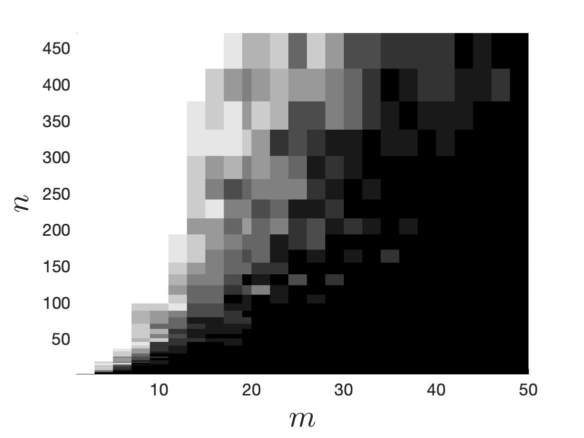
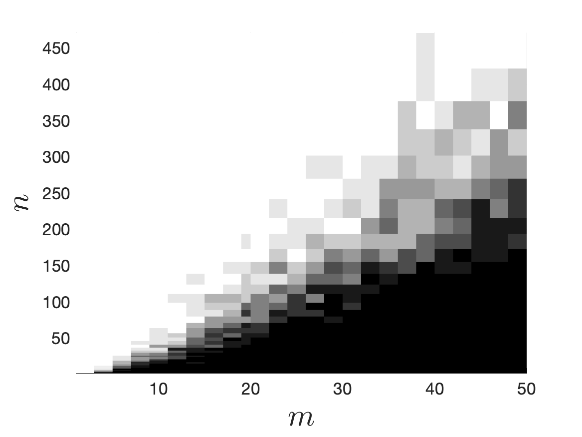
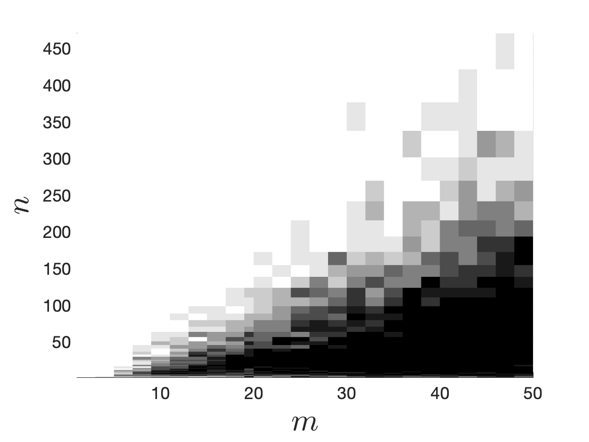
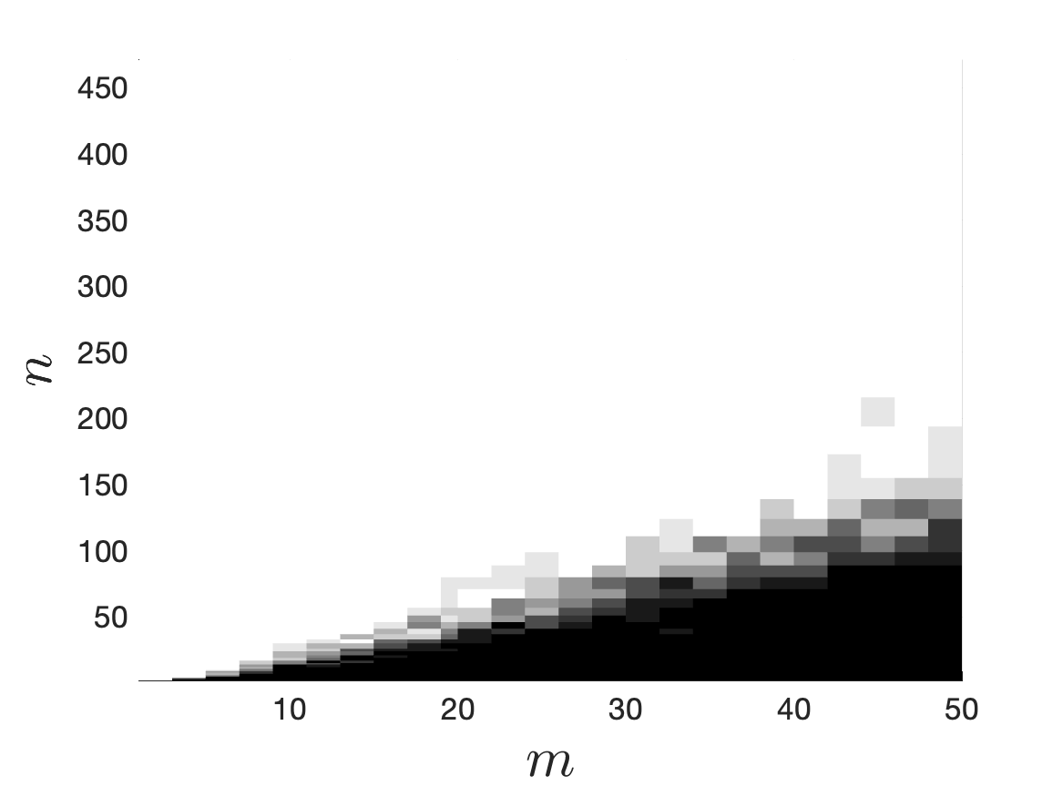
Figure 2 illustrates the same quantities for the case of the standard gaussian measure $\mu$ over $\mathcal{X}=\mathbb{R}$. We draw essentially the same conclusions. We notice in this case the very poor performance of classical sampling from $\mu$.

(a)

(b)

(c)

(d)

Figure 2: For $V_{m}$ the space of polynomials of degree $m-1$ and $\mu$ the standard gaussian measure on $\mathbb{R}$, we plot $\mathbb{P}(\lambda_{min}(\mathbf{G}^{w})\geq 1/4)$ as a function of dimension $m$ and number of samples $n.$ Probability estimates go from 0 (black) to 1 (white).

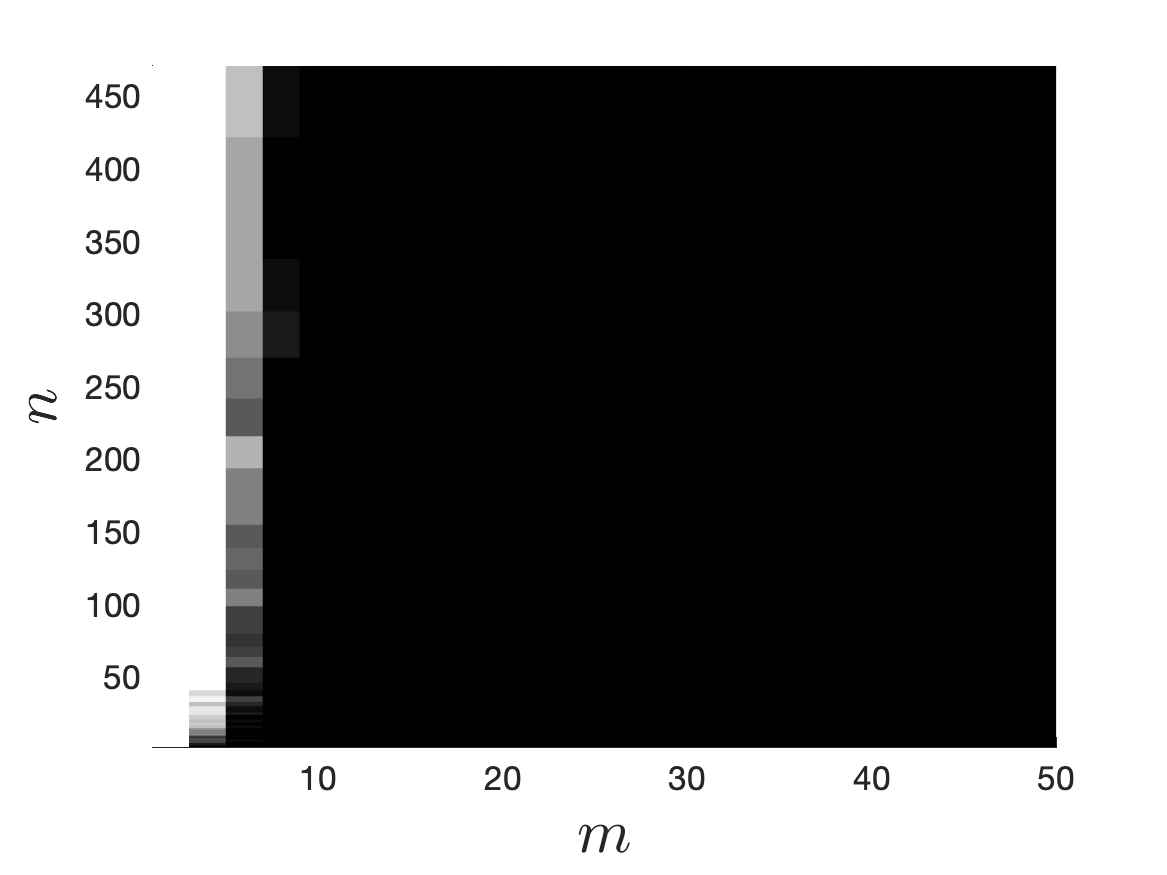
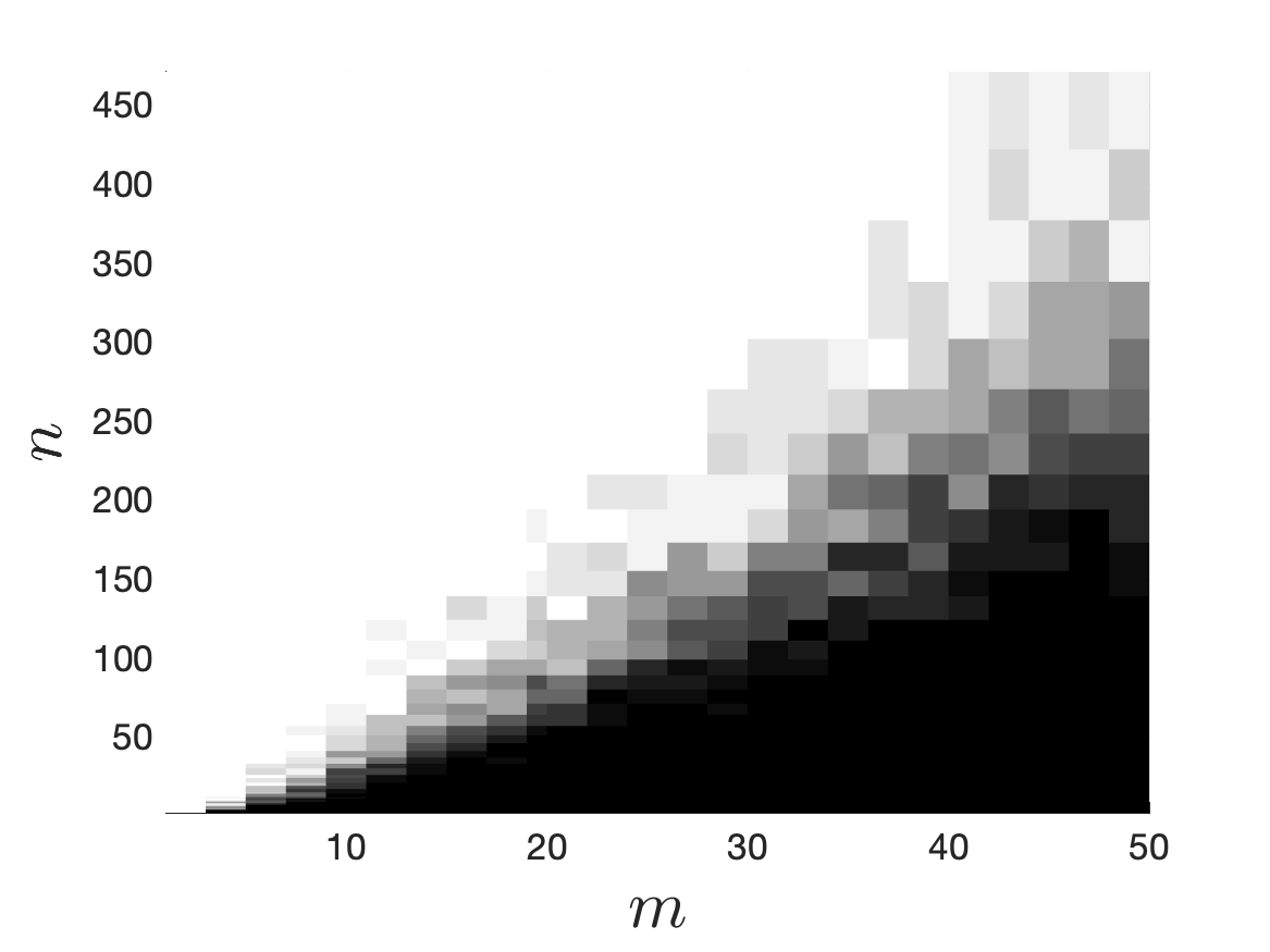
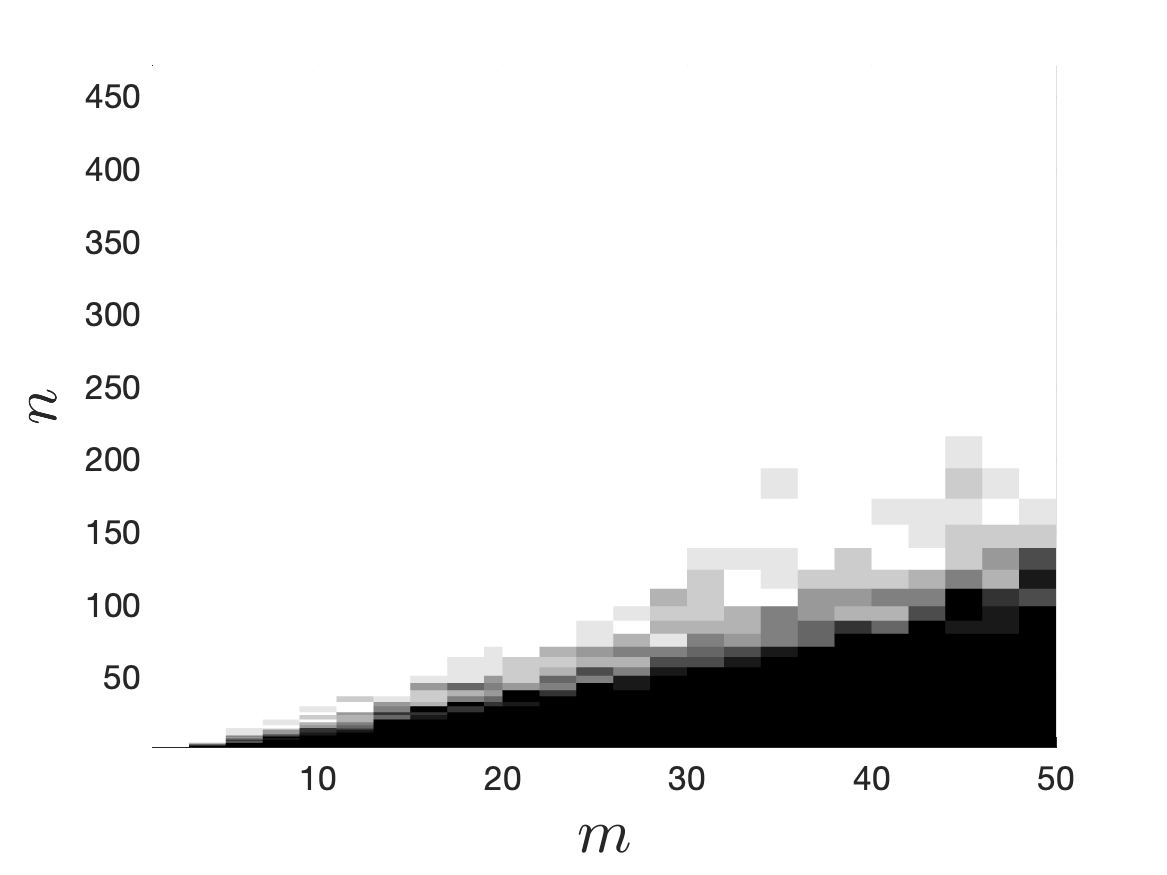
From now on, we consider the approximation of the function $f(x)=(1+2x^{2})^{-1}$ on $\mathbb{R}$ equipped with the standard gaussian measure $\mu$, and $V_{m}$ the space of polynomials of degree $m-1$. On Figure 3, we plot the histograms of the logarithm of the $L^{2}_{\mu}$ relative error, $\log(\|f-\hat{f}_{m}\|/\|f\|)$, for the different sampling strategies and using $n=rm$ for different $r$. For small oversampling ($r=2$), we observe the benefit of volume-rescaled sampling over i.i.d. sampling, which shifts the distribution towards small values. We also observe a clear superiority of repeated DPP $\gamma_{m}^{\otimes r}$, which is further improved by conditioning to satisfy the event $S_{\delta}$ with $\delta=3/4$. For large oversampling ($r=10$), the histograms are roughly similar. We only observe a slight benefit of conditioned repeated DPP over the other methods, even over i.i.d. optimal sampling.

(a)

(b)

(c)

Figure 3: For $V_{m}$ the space of polynomials of degree $m-1$ and $\mu$ the standard gaussian measure on $\mathbb{R}$, we plot the histogram of $\log(\|f-\hat{f}_{m}\|/\|f\|)$ using $n=rm$ samples from $\nu_{m}^{\otimes n}$ (blue), the volume-rescaled sampling distribution $\gamma_{n}^{\nu_{m}}$ (green), repeated DPP $\gamma_{m}^{\otimes r}$ (red), or repeated DPP conditioned to satisfy $S_{\delta}$ with $\delta=3/4$.

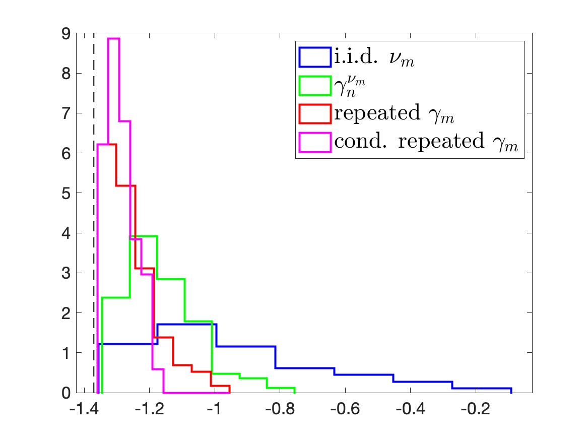
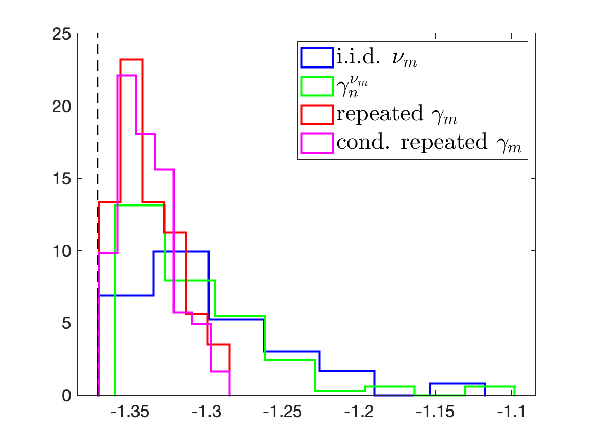
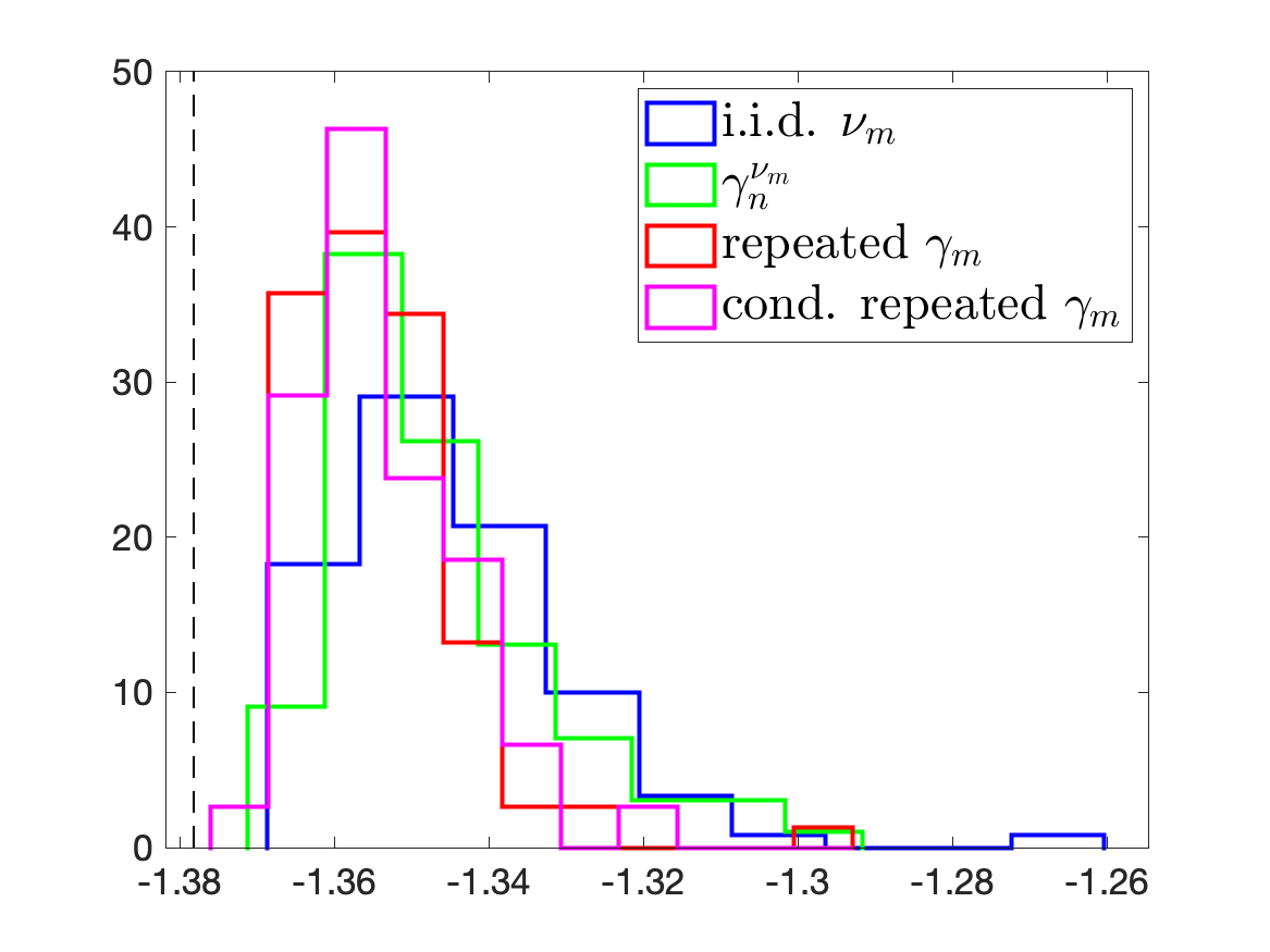
Table 1 show the expected relative error $\mathbb{E}(\|f-\hat{f}_{m}\|^{2})^{1/2}/\|f\|$ and the quantile of $\|f-\hat{f}_{m}\|/\|f\|$ of level $95\%$. We first observe the catastrophic results for classical i.i.d. sampling from $\mu.$ For small oversampling ($n=2m$), we observe on both criteria a clear benefit of volume-rescaled and repeated DPP over i.i.d. sampling. In terms of expected error, we observe a slight improvement of repeated DPP compared to volume-rescaled sampling. However, concerning the quantile, we observe a clear superiority of repeated DPP over volume-rescaled sampling. For the same number of samples, this quantile is divided by up to a factor 2. For larger oversampling ($n=5m$), i.i.d. performs much better and gets closer to the performance of volume-rescaled sampling and repeated DPP.

$$\begin{array}[]{|c|c|c|c|c|c|c|}\hline\cr m&\text{best}&\text{i.i.d. $\mu$}&\text{i.i.d. $\nu_{m}$}&\text{$\gamma_{n}^{\nu_{m}}$}&\text{$\gamma_{m}^{\otimes n/m}$}&\text{$\gamma_{m}^{\otimes n/m}$ (cond.)}\\ \hline\cr 10&1.3e-01&7.8e+02&3.9e-01&2.0e-01&1.8e-01&1.6e-01\\ \hline\cr 20&5.1e-02&3.4e+07&1.9e-01&7.7e-02&6.6e-02&6.2e-02\\ \hline\cr 30&2.5e-02&6.3e+08&1.0e-01&3.9e-02&3.2e-02&3.0e-02\\ \hline\cr 40&1.3e-02&5.1e+08&6.2e-02&2.2e-02&1.7e-02&1.6e-02\\ \hline\cr 50&8.0e-03&3.8e+09&6.5e-02&1.4e-02&1.0e-02&9.6e-03\\ \hline\cr\end{array}$$

(a) $n=2m$. Expected relative error $\mathbb{E}(\|f-\hat{f}_{m}\|^{2})^{1/2}/\|f\|$.

$$\begin{array}[]{|c|c|c|c|c|c|c|}\hline\cr m&\text{best}&\text{i.i.d. $\mu$}&\text{i.i.d. $\nu_{m}$}&\text{$\gamma_{n}^{\nu_{m}}$}&\text{$\gamma_{m}^{\otimes n/m}$}&\text{$\gamma_{m}^{\otimes n/m}$ (cond.)}\\ \hline\cr 10&1.3e-01&3.0e+03&8.8e-01&3.3e-01&2.6e-01&2.1e-01\\ \hline\cr 20&5.1e-02&1.4e+08&7.0e-01&1.1e-01&8.8e-02&8.0e-02\\ \hline\cr 30&2.5e-02&2.4e+09&3.2e-01&6.8e-02&4.2e-02&3.7e-02\\ \hline\cr 40&1.3e-02&1.6e+09&1.8e-01&3.7e-02&2.4e-02&2.1e-02\\ \hline\cr 50&8.0e-03&1.3e+10&1.3e-01&2.6e-02&1.4e-02&1.2e-02\\ \hline\cr\end{array}$$

(b) $n=2m$. Quantile of $\|f-\hat{f}_{m}\|/\|f\|$ of level $95\%$.

$$\begin{array}[]{|c|c|c|c|c|c|c|}\hline\cr m&\text{best}&\text{i.i.d. $\mu$}&\text{i.i.d. $\nu_{m}$}&\text{$\gamma_{n}^{\nu_{m}}$}&\text{$\gamma_{m}^{\otimes n/m}$}&\text{$\gamma_{m}^{\otimes n/m}$ (cond.)}\\ \hline\cr 10&1.3e-01&4.9e+01&1.5e-01&1.5e-01&1.4e-01&1.4e-01\\ \hline\cr 20&5.0e-02&2.7e+05&5.9e-02&5.7e-02&5.4e-02&5.4e-02\\ \hline\cr 30&2.4e-02&2.9e+07&2.9e-02&2.8e-02&2.6e-02&2.6e-02\\ \hline\cr 40&1.3e-02&3.6e+08&1.6e-02&1.5e-02&1.4e-02&1.4e-02\\ \hline\cr 50&7.9e-03&1.1e+09&9.5e-03&9.0e-03&8.6e-03&8.5e-03\\ \hline\cr\end{array}$$

(c) $n=5m$. Expected relative error $\mathbb{E}(\|f-\hat{f}_{m}\|^{2})^{1/2}/\|f\|$.

$$\begin{array}[]{|c|c|c|c|c|c|c|}\hline\cr m&\text{best}&\text{i.i.d. $\mu$}&\text{i.i.d. $\nu_{m}$}&\text{$\gamma_{n}^{\nu_{m}}$}&\text{$\gamma_{m}^{\otimes n/m}$}&\text{$\gamma_{m}^{\otimes n/m}$ (cond.)}\\ \hline\cr 10&1.3e-01&1.5e+02&1.8e-01&1.8e-01&1.6e-01&1.5e-01\\ \hline\cr 20&5.0e-02&1.2e+06&7.5e-02&6.7e-02&6.1e-02&6.0e-02\\ \hline\cr 30&2.4e-02&1.4e+08&3.8e-02&3.3e-02&2.9e-02&3.0e-02\\ \hline\cr 40&1.3e-02&1.3e+09&2.1e-02&1.8e-02&1.6e-02&1.6e-02\\ \hline\cr 50&7.9e-03&4.2e+09&1.3e-02&1.0e-02&9.5e-03&9.2e-03\\ \hline\cr\end{array}$$

(d) $n=5m$. Quantile of $\|f-\hat{f}_{m}\|/\|f\|$ of level $95\%$.

Table 1: For $V_{m}$ the space of polynomials of degree $m-1$ and $\mu$ the standard gaussian measure on $\mathbb{R}$, we indicate the expected relative error or the quantile of the relative error of level 95%, using $n=rm$ samples from $\nu_{m}^{\otimes n}$ (blue), the volume-rescaled distribution $\gamma_{n}^{\nu_{m}}$ (green), repeated DPP $\gamma_{m}^{\otimes r}$ (red), or repeated DPP conditioned to $S_{\delta}$ with $\delta=3/4$. The column “best” indicates the best approximation error in $V_{m}.$

The above numerical experiments illustrate the superiority of repeated DPP distribution $\gamma_{m}^{\otimes r}$ over i.i.d. optimal sampling, but also over volume-rescaled sampling, in the small oversampling regime. for large oversampling, the different sampling strategies yield similar results. The interest of repeated DPP distribution is that for very small oversampling, stability $S_{\delta}$ can be achieved with a reasonable probability. This allows for sampling conditioned to $S_{\delta}$, which further improves the quality of the least-squares projection.

Appendix A Some known results on random matrices

Theorem A.1 (Matrix Chernoff inequality [22]).

Let $\mathbf{A}_{1},\ldots\mathbf{A}_{n}$ be independent random symmetric matrices of size $m$-by-$m$ such that for all $i$, $0\leq\lambda_{min}(\mathbf{A}_{i})$ and $\lambda_{max}(\mathbf{A}_{i})\leq L$. Then

$$\mathbb{P}(\lambda_{max}(\sum_{i=1}^{n}\mathbf{A}_{i})\geq(1+\delta)\mu_{max})\leq m\exp(-d_{\delta}\mu_{max}/L)\quad\text{for }\epsilon\geq 0,\quad\text{and}$$ (17)

$$\mathbb{P}(\lambda_{min}(\sum_{i=1}^{n}\mathbf{A}_{i})\leq(1-\delta)\mu_{min})\leq m\exp(-c_{\delta}\mu_{min}/L)\quad\text{for }\epsilon\in[0,1),$$ (18)

where $\mu_{min}=\lambda_{min}(\mathbb{E}(\sum_{i=1}^{n}\mathbf{A}_{i}))$, $\mu_{max}=\lambda_{max}(\mathbb{E}(\sum_{i=1}^{n}\mathbf{A}_{i}))$, $c_{\delta}=\delta+(1-\delta)\log(1-\delta)$ and $d_{\delta}=-\delta+(1+\delta)\log(1+\delta).$ It holds $\frac{5}{13}\delta^{2}\leq d_{\delta}\leq\delta^{2}/2\leq c_{\delta}\leq\delta^{2}$.

Proof.

We provide a sketch of the proof of Tropp [tropp2015introduction] for the bound on the minimal eigenvalue. Let $\mathbf{B}=\sum_{i=1}^{n}\mathbf{A}_{i}$. For any $\theta<0$, it holds

$$\mathbb{P}(\lambda_{min}(\mathbf{B})\leq t)=\mathbb{P}(e^{\theta\lambda_{min}(\mathbf{B})}\geq e^{\theta t})=\mathbb{P}(e^{\lambda_{min}(\theta\mathbf{B})}\geq e^{\theta t})\leq e^{-\theta t}\mathbb{E}(e^{\lambda_{min}(\theta\mathbf{B})}),$$

where the last inequality is given by Markov inequality. Then using $e^{\lambda_{min}(\theta\mathbf{B})}=\lambda_{min}(e^{\theta\mathbf{B}})\leq\mathrm{tr}(e^{\theta\mathbf{B}})$, we obtain

$$\mathbb{P}(\lambda_{min}(\mathbf{B})\leq t)\leq\inf_{\theta<0}e^{-\theta t}\mathbb{E}(\mathrm{tr}e^{\theta\mathbf{B}}).$$

For positive-definite matrix $\mathbf{H}$, the map $\mathbf{A}\mapsto\mathrm{tr}e^{\mathbf{H}+\log(\mathbf{A})}$ is concave on the positive cone of positive definite matrices. Letting $\mathbf{X}_{i}:=e^{\theta\mathbf{A}_{i}}$, a sequential application of Jensen’s inequality gives

$$\mathbb{E}(\mathrm{tr}e^{\theta\mathbf{B}})=\mathbb{E}(\mathrm{tr}\exp(\sum_{i=1}^{n}\log(\mathbf{X}_{i})))\leq\mathrm{tr}\exp(\sum_{i=1}^{n}\log(\mathbb{E}(\mathbf{X}_{i})))=\mathrm{tr}\exp(\sum_{i=1}^{n}\log(\mathbb{E}(e^{\theta\mathbf{A}_{i}}))).$$

Also it holds $\log\mathbb{E}(e^{\theta\mathbf{A}_{i}})\preceq g(\theta)\mathbb{E}(\mathbf{A}_{i})$ where $g(\theta)=L^{-1}(e^{\theta L}-1),$ so that

$$\mathrm{tr}\exp(\sum_{i=1}^{n}\log(\mathbb{E}(e^{\theta\mathbf{A}_{i}})))\leq\mathrm{tr}\exp(g(\theta)\mathbb{E}(\sum_{i=1}^{n}\mathbf{A}_{i}))\leq ne^{g(\theta)\mu_{min}}.$$

Therefore,

$$\mathbb{P}(\lambda_{min}(\mathbf{B})\leq t)\leq\inf_{\theta<0}ne^{-\theta t}e^{g(\theta)\mu_{min}}$$

Taking $t=(1-\delta)\mu_{min}$, the infimum is attained at $\theta=L^{-1}\log(1-\delta)$, which gives the desired result. ∎

Lemma A.2 (Lemma 2.3 in [7]).

Let $\mathbf{A},\mathbf{B}\in\mathbb{R}^{n\times m}$ be two random matrices whose row vectors are drawn as an i.i.d. sequence of $n$ pairs of random vectors $(\mathbf{a}_{i},\mathbf{b}_{i})$. Then

$$n^{m}\mathbb{E}(\det(\mathbf{A}^{T}\mathbf{B}))= \frac{n!}{(n-m)!}\det(\mathbb{E}(\mathbf{A}^{T}\mathbf{B}))\quad\text{for any }n\geq m,\;\text{and}$$

$$n^{m-1}\mathbb{E}(\mathrm{adj}(\mathbf{A}^{T}\mathbf{B}))= \frac{n!}{(n-m+1)!}\mathrm{adj}(\mathbb{E}(\mathbf{A}^{T}\mathbf{B}))\quad\text{for any }n\geq m-1.$$

Lemma A.3 (Lemma 2.11 in [7]).

For any matrix $\mathbf{A}\in\mathbb{R}^{n\times m}$ with $n>m,$ it holds

$$\det(\mathbf{A}^{T}\mathbf{A})\mathbf{A}^{\dagger}=\frac{n}{n-m}\sum_{i=1}^{n}\det(\mathbf{A}^{T}(\mathbf{I}-\mathbf{e}_{i}\mathbf{e}_{i}^{T})\mathbf{A})((\mathbf{I}-\mathbf{e}_{i}\mathbf{e}_{i}^{T})\mathbf{A})^{\dagger}.$$

Appendix B Properties of projection determinental point processes

Proof of proposition 4.1.

This is a standard result on projection determinantal processes, see e.g. [15]. We here provide a short proof with our notations. The fact that all marginals are the same comes from the invariance to permutations of the distribution $\gamma_{m}$. From the classical ”base times height formula” for a determinant, we have

$$\det(\Phi(\mathbf{x}))=\det((\boldsymbol{\varphi}(x_{1}),\ldots\boldsymbol{\varphi}(x_{m})))=\|\boldsymbol{\varphi}(x_{1})\|_{2}\|P_{W_{1}^{\perp}}\boldsymbol{\varphi}(x_{2})\|_{2}\ldots\|P_{W_{m-1}^{\perp}}\boldsymbol{\varphi}(x_{m})\|_{2}$$

with $P_{W_{k}^{\perp}}=I_{m}-P_{W_{k}}$ the orthogonal projection onto the orthogonal complement of $W_{k}=span\{\boldsymbol{\varphi}(x_{1}),\ldots,\boldsymbol{\varphi}(x_{k})\}$ in $\mathbb{R}^{m}$. Therefore, the density of $\gamma_{m}$ with respect to $\mu^{\otimes m}$ has the following expression

$$\frac{1}{m!}\det(\Phi(\mathbf{x})^{T}\Phi(\mathbf{x}))=\prod_{k=1}^{m}p_{k}(x_{k}),\quad p_{k}(x_{k}):=\frac{1}{m-k+1}\|P_{W_{k-1}^{\perp}}\boldsymbol{\varphi}(x_{k})\|^{2}_{2},$$

with the convention $W_{0}=\{0\}.$ The function $p_{k}$ depends on $(x_{1},\ldots,x_{k-1})$ and is a density since

$$\int p_{k}(x)d\mu(x) =\frac{1}{m-k+1}\int\boldsymbol{\varphi}(x)^{T}P_{W_{k-1}^{\perp}}\boldsymbol{\varphi}(x)d\mu(x)$$

$$=\frac{1}{m-k+1}\mathrm{tr}(P_{W_{k-1}^{\perp}}\int\boldsymbol{\varphi}(x)\boldsymbol{\varphi}(x)^{T}d\mu(x))$$

$$=\frac{1}{m-k+1}\mathrm{tr}(P_{W_{k-1}^{\perp}})=1,$$

where we have used the fact that $\mathrm{tr}(P_{W_{k-1}^{\perp}})=\dim(W_{k-1}^{\perp})=m-k+1.$ That provides a factorization of $\gamma_{m}$ in terms of the marginal $p_{1}(x_{1})d\mu(x_{1})=\frac{1}{m}\|\boldsymbol{\varphi}(x_{1})\|_{2}^{2}d\mu$ and the conditional distributions $p_{k}(x_{k})d\mu(x_{k})$ of $x_{k}$ knowing $(x_{1},\ldots,x_{k-1}),$ which ends the proof.

∎

The next result provides the distribution of all marginal distributions of $\gamma_{m}$.

Proposition B.1.

Let $\mathbf{x}=(x_{1},\ldots,x_{m})\sim\gamma_{m}$. For a nonempty tuple $T\subset[m]$, $\mathbf{x}_{T}=(x_{i})_{i\in T}$ has for distribution

$$\frac{(m-|T|)!}{m!}\det(\Phi(\mathbf{y})\Phi(\mathbf{y})^{T})d\mu^{\otimes|T|}(\mathbf{y}),\quad\mathbf{y}\in\mathcal{X}^{|T|}.$$

Proof.

Because of the symmetry of the distribution $\gamma_{m}$, it is sufficient to consider sets $T=[k]$ and $\mathbf{x}_{T}=\mathbf{x}_{[k]}=(x_{1},\ldots,x_{k})$. Let denote $p_{[k]}\mu^{\otimes k}$ the distribution of $\mathbf{x}_{[k]}$. The result is true for $k=1$. Then we proceed by induction. From Proposition 4.1, we know that the conditional distribution of $x_{k+1}$ knowing $\mathbf{x}_{[k]}$ is

$$\frac{1}{m-k}(\|\boldsymbol{\varphi}(x_{k+1})\|^{2}_{2}-\|\Phi(\mathbf{x}_{[k]})(\Phi(\mathbf{x}_{[k]})\Phi(\mathbf{x}_{[k]})^{T})^{-1}\Phi(\mathbf{x}_{[k]})^{T}\boldsymbol{\varphi}(x_{k+1})\|_{2}^{2})d\mu.$$

Assuming the distribution of $\mathbf{x}_{[k]}$ is

$$\frac{(m-k)!}{m!}\det(\Phi(\mathbf{x}_{[k]})\Phi(\mathbf{x}_{[k]})^{T})d\mu^{\otimes k}(\mathbf{x}_{[k]}),$$

we deduce that the distribution of $\mathbf{x}_{[k+1]}=(\mathbf{x}_{[k]},x_{k+1})$ admits as density with respect to $\mu^{\otimes(k+1)}$

$$\frac{(m-k-1)!}{m!}\det(\Phi(\mathbf{x}_{[k]})\Phi(\mathbf{x}_{[k]})^{T})(\|\boldsymbol{\varphi}(x_{k+1})\|^{2}_{2}$$

$$\quad-\|\Phi(\mathbf{x}_{[k]})(\Phi(\mathbf{x}_{[k]})\Phi(\mathbf{x}_{[k]})^{T})^{-1}\Phi(\mathbf{x}_{[k]})^{T}\boldsymbol{\varphi}(x_{k+1})\|_{2}^{2})$$

$$=\frac{(m-k-1)!}{m!}\det(\Phi(\mathbf{x}_{[k]})\Phi(\mathbf{x}_{[k]})^{T})(\boldsymbol{\varphi}(x_{k+1})^{T}\boldsymbol{\varphi}(x_{k+1})$$

$$\quad-\boldsymbol{\varphi}(x_{k+1})^{T}\Phi(\mathbf{x}_{[k]})(\Phi(\mathbf{x}_{[k]})\Phi(\mathbf{x}_{[k]})^{T})^{-1}\Phi(\mathbf{x}_{[k]})^{T}\boldsymbol{\varphi}(x_{k+1}))$$

$$=\frac{(m-k-1)!}{m!}\det(\Phi(\mathbf{x}_{[k+1]})\Phi(\mathbf{x}_{[k+1]}^{T})),$$

which ends the proof.

∎

Appendix C Properties of volume sampling

We first provide a straightforward result.

Lemma C.1.

For any measurable function $g:\mathcal{X}^{n}\to\mathbb{R},$

$$\mathbb{E}_{\mathbf{x}\sim\gamma_{n}^{\nu}}(g(\mathbf{x}))=\mathbb{E}_{\mathbf{y}\sim\nu^{\otimes n}}(\frac{(n-m)!}{n!}\det(\Phi^{w}(\mathbf{y})^{T}\Phi^{w}(\mathbf{y}))g(\mathbf{y})).$$

Lemma C.2.

Assume $(x_{1},\ldots,x_{n})$ is drawn from the distribution $\gamma_{n}^{\nu}$ with $\nu=w\mu$. Then for any function $f$, it holds

$$\mathbb{E}(\Phi^{w}(\mathbf{x})^{\dagger}f^{w}(\mathbf{x}))=\mathbb{E}_{y\sim\mu}(\boldsymbol{\varphi}(y)f(y))$$

where $f^{w}=fw^{-1/2}.$

Proof.

First consider the case $n=m$, where $\mathbf{x}=(x_{1},\ldots,x_{m})$ is drawn from $\gamma_{m}=\mathrm{DPP}_{\mu}(V_{m}).$ In this case, $\Phi(\mathbf{x})$ is a square matrix, almost surely invertible, and $\Phi^{w}(\mathbf{x})^{\dagger}f^{w}(\mathbf{x})=\Phi(\mathbf{x})^{\dagger}f(\mathbf{x})$. Noting $\mathbf{y}\sim\mu^{\otimes m}$, we obtain using Cramer’s rule

$$\mathbb{E}(\Phi(\mathbf{x})^{\dagger}f(\mathbf{x}))_{i} =\frac{1}{m!}\mathbb{E}(\det(\Phi(\mathbf{y})^{T}\Phi(\mathbf{y}))\Phi(\mathbf{y})^{\dagger}f(\mathbf{y}))_{i}$$

$$=\frac{1}{m!}\mathbb{E}(\det(\Phi(\mathbf{y})^{T})\det(\Phi(\mathbf{y})+(f(\mathbf{y})-\Phi(\mathbf{y})\mathbf{e}_{i})\mathbf{e}_{i}^{T}))$$

$$=\frac{1}{m!}\mathbb{E}(\det(\Phi(\mathbf{y})^{T}(\Phi(\mathbf{y})+(f(\mathbf{y})-\Phi(\mathbf{y})\mathbf{e}_{i})\mathbf{e}_{i}^{T})))$$

$$\overset{(*)}{=}\det(\frac{1}{m}\mathbb{E}(\Phi(\mathbf{y})^{T}(\Phi(\mathbf{y})+(f(\mathbf{y})-\Phi(\mathbf{y})\mathbf{e}_{i})\mathbf{e}_{i}^{T})))$$

$$=\det(\mathbf{I}+(\mathbb{E}_{y\sim\mu}(\boldsymbol{\varphi}(y)f(y))-\mathbf{e}_{i})\mathbf{e}_{i}^{T})=(\mathbb{E}_{y\sim\mu}(\boldsymbol{\varphi}(y)f(y)))_{i},$$

where $(*)$ is deduced from Lemma A.2. For the case $n>m$, we proceed by induction. Letting $\mathbf{y}\sim\nu^{\otimes n}$ and using Lemma A.3, we have

$$\mathbb{E}(\Phi^{w}(\mathbf{x})^{\dagger}f^{w}(\mathbf{x})) =\frac{(n-m)!}{n!}\mathbb{E}(\det(\Phi^{w}(\mathbf{y})^{T}\Phi^{w}(\mathbf{y}))\Phi^{w}(\mathbf{y})^{\dagger}f^{w}(\mathbf{y}))$$

$$=\frac{(n-m)!}{n!}\frac{n}{n-m}\sum_{i=1}^{n}\mathbb{E}(\det(\Phi^{w}(\mathbf{y})^{T}(\mathbf{I}-\mathbf{e}_{i}\mathbf{e}_{i}^{T})\Phi^{w}(\mathbf{y}))((\mathbf{I}-\mathbf{e}_{i}\mathbf{e}_{i}^{T})\Phi^{w}(\mathbf{y}))^{\dagger}f^{w}(\mathbf{y}))$$

$$=\frac{(n-m-1)!}{(n-1)!}\sum_{i=1}^{n}\mathbb{E}(\det(\Phi^{w}(\mathbf{y}_{-i})^{T}\Phi^{w}(\mathbf{y}_{-i}))(\Phi^{w}(\mathbf{y}_{-i}))^{\dagger}f^{w}(\mathbf{y}_{-i}))$$

$$=\mathbb{E}(\Phi^{w}(\tilde{\mathbf{x}})^{-1}f^{w}(\tilde{\mathbf{x}})),$$

with $\tilde{\mathbf{x}}\sim\gamma_{n-1}^{\nu},$ and $\mathbf{y}_{-i}$ is the vector $\mathbf{y}$ without the $i$-th component. We then deduce $\mathbb{E}(\Phi^{w}(\mathbf{x})^{\dagger}f^{w}(\mathbf{x}))=\mathbb{E}_{y\sim\mu}(\boldsymbol{\varphi}(y)f(y))$.
∎

Lemma C.3.

Assume $(x_{1},\ldots,x_{n})$ is drawn from the distribution $\gamma_{n}^{\nu}$ with $\nu=w\mu$ and $w\geq\alpha w_{m}$. Then for any function $f$ and $f^{w}=fw^{-1/2}$, it holds

$$\mathbb{E}(\|\frac{1}{n}\Phi^{w}(\mathbf{x})^{T}f^{w}(\mathbf{x})\|^{2}) \leq\frac{m}{n}\alpha^{-1}(\beta+\xi m\alpha^{-1})\|f\|^{2}+\|P_{V_{m}}f\|^{2}$$

with $\beta=1+(\alpha^{-1}-1)\frac{m}{n}$ and $\xi=0$ if $\nu=\nu_{m}$ or $\xi=1$ if $\nu\neq\nu_{m}$. In the case where $\boldsymbol{\varphi}(x_{i})f(x_{i})\geq 0$ almost surely, it holds

$$\mathbb{E}(\|\frac{1}{n}\Phi^{w}(\mathbf{x})^{T}f^{w}(\mathbf{x})\|^{2}) \leq\frac{m}{n}\alpha^{-1}\beta\|f\|^{2}+(1+2\alpha^{-2}\frac{m}{n})\|P_{V_{m}}f\|^{2}$$

Proof.

Let $\mathbf{b}=\frac{1}{n}\Phi^{w}(\mathbf{x})^{T}f^{w}(\mathbf{x})=\frac{1}{n}\sum_{k=1}^{n}\boldsymbol{\varphi}(x_{k})^{T}f(x_{k})w(x_{k})^{-1}.$ Letting $\mathbf{a}(x):=\boldsymbol{\varphi}(x)f(x)w(x)^{-1}$, we have

$$\mathbb{E}(\|\mathbf{b}\|_{2}^{2}) =\frac{1}{n^{2}}\sum_{k,l=1}^{n}\mathbb{E}((\mathbf{a}(x_{k}),\mathbf{a}(x_{l})))=\frac{1}{n^{2}}\sum_{k=1}^{n}\mathbb{E}(\|\mathbf{a}(x_{k})\|^{2})+\frac{1}{n^{2}}\sum_{\begin{subarray}{c}k,l=1\\ k\neq l\end{subarray}}^{n}\mathbb{E}((\mathbf{a}(x_{k}),\mathbf{a}(x_{l})))$$

The marginal distribution of $\gamma_{n}^{\nu}$ is $\tilde{\nu}=\tilde{w}\mu$ with $\tilde{w}=\frac{n-m}{n}w+\frac{m}{n}w_{m}$ such that $\tilde{w}\leq\beta w$ with $\beta=1+(\alpha^{-1}-1)\frac{m}{n}$. Then,

$$\frac{1}{n^{2}}\sum_{k=1}^{n}\mathbb{E}(\|\mathbf{a}(x_{k})\|^{2}) =\frac{1}{n}\mathbb{E}_{x\sim\tilde{\nu}}(\|\boldsymbol{\varphi}(x)\|_{2}^{2}f(x)^{2}w(x)^{-2})$$

$$\leq\frac{m}{n}\alpha^{-1}\beta\,\mathbb{E}_{x\sim\tilde{\nu}}(f(x)^{2}\tilde{w}(x)^{-1})$$

$$=\frac{m}{n}\alpha^{-1}\beta\|f\|^{2}.$$

Up to a permutation, we can now consider that $(x_{1},\ldots,x_{m})\sim\gamma_{m}$ and $(x_{m+1},\ldots,x_{n})\sim\nu^{\otimes(n-m)}$ are independent. Letting $z\sim\nu$, $y\sim\mu$, we have

$$\mathbb{E}(\sum_{\begin{subarray}{c}k,l=1\\ k\neq l\end{subarray}}^{n}(\mathbf{a}(x_{k}),\mathbf{a}(x_{l})))=m(m-1)\mathbb{E}((\mathbf{a}(x_{1}),\mathbf{a}(x_{2})))$$

$$\quad+2m(n-m)(\mathbb{E}(\mathbf{a}(x_{1})),\mathbb{E}(\mathbf{a}(z)))+(n-m)(n-m-1)\|\mathbb{E}(\mathbf{a}(z))\|^{2}_{2}$$

We have

$$\|\mathbb{E}(\mathbf{a}(z))\|_{2}=\|\mathbb{E}(\boldsymbol{\varphi}(z)f(z)w(z)^{-1})\|_{2}=\|\mathbb{E}(\boldsymbol{\varphi}(y)f(y))\|_{2}^{2}=\|P_{V_{m}}f\|_{2}.$$

Letting $(y_{1},y_{2})\sim\mu^{\otimes 2}$, and using Proposition B.1, we obtain

$$m(m-1)\mathbb{E}((\mathbf{a}(x_{1}),\mathbf{a}(x_{2}))) =\mathbb{E}((\mathbf{a}(y_{1}),\mathbf{a}(y_{2}))\det(\Phi(y_{1},y_{2})\Phi(y_{1},y_{2})^{T}))$$

$$=\mathbb{E}((\mathbf{a}(y_{1}),\mathbf{a}(y_{2}))(\|\boldsymbol{\varphi}(y_{1})\|^{2}\|\boldsymbol{\varphi}(y_{2})\|^{2}-(\boldsymbol{\varphi}(y_{1}),\boldsymbol{\varphi}(y_{2}))^{2}))$$

$$\leq\|\mathbb{E}(\mathbf{a}(y_{1})\|\boldsymbol{\varphi}(y_{1})\|^{2})\|_{2}^{2}$$

$$\quad-\mathbb{E}((\boldsymbol{\varphi}(y_{1}),\boldsymbol{\varphi}(y_{2}))^{3}f(y_{1})f(y_{2})w(y_{1})^{-1}w(y_{2})^{-1})$$

The second term in the above upper bound can be written $\mathbb{E}(\sum_{l}g_{l}(y_{1})g_{l}(y_{2}))=\sum_{l}\mathbb{E}(g_{l}(y))^{2}$ for some functions $g_{l}$, so that

$$m(m-1)(\mathbb{E}(\mathbf{a}(x_{1})),\mathbb{E}(\mathbf{a}(x_{2}))) \leq m^{2}\|\mathbb{E}(\mathbf{a}(x))\|_{2}^{2},$$

with $x\sim\nu_{m}$. Gathering the above results, we get

$$\mathbb{E}(\|\mathbf{b}\|_{2}^{2})\leq \frac{m}{n}\alpha^{-1}\beta\|f\|^{2}+\frac{m^{2}}{n^{2}}\|\mathbb{E}(\mathbf{a}(x))\|_{2}^{2}$$

$$+\frac{2m(n-m)}{n^{2}}\|\mathbb{E}(\mathbf{a}(x))\|_{2}\|P_{V_{m}}f\|+\frac{(n-m)(n-m-1)}{n^{2}}\|P_{V_{m}}f\|^{2}.$$

If $w=w_{m}$, then $\alpha=\beta=1$ and $\|\mathbb{E}(\mathbf{a}(x))\|_{2}=\|P_{V_{m}}f\|$, and therefore

$$\mathbb{E}(\|\mathbf{b}\|_{2}^{2}) \leq\frac{m}{n}\|f\|^{2}+\frac{m^{2}+2m(n-m)+(n-m)(n-m-1)}{n^{2}}\|P_{V_{m}}f\|^{2}$$

$$\leq\frac{m}{n}\|f\|^{2}+\frac{n^{2}-n+m}{n^{2}}\|P_{V_{m}}f\|^{2}\leq\frac{m}{n}\|f\|^{2}+(1-\frac{n-m}{n^{2}})\|P_{V_{m}}f\|^{2}$$

If $w\geq\alpha w_{m}$, we have

$$\|\mathbb{E}(\mathbf{a}(x))\|_{2}\leq\mathbb{E}(\|\mathbf{a}(x)\|_{2}^{2})^{1/2}=m^{1/2}\mathbb{E}(f(y)^{2}w(y)^{-2}w_{m}(y)^{2})^{1/2}\leq m^{1/2}\alpha^{-1}\|f\|,$$

and therefore, letting $\xi_{m}=m^{1/2}$,

$$\mathbb{E}(\|\mathbf{b}\|_{2}^{2}) \leq\frac{m}{n}\alpha^{-1}\beta\|f\|^{2}+\frac{m^{2}}{n^{2}}\xi_{m}^{2}\alpha^{-2}\|f\|^{2}$$

$$\quad+\frac{2m(n-m)}{n^{2}}\xi_{m}\alpha^{-1}\|f\|\|P_{V_{m}}f\|+\frac{(n-m)(n-m-1)}{n^{2}}\|P_{V_{m}}f\|^{2}$$

$$\leq(\frac{m}{n}\alpha^{-1}\beta+\frac{m}{n}\xi_{m}^{2}\alpha^{-2})\|f\|^{2}+\frac{(n-m)(n-m-1)+m(n-m)}{n^{2}}\|P_{V_{m}}f\|^{2}$$

$$\leq\frac{m}{n}\alpha^{-1}(\beta+\xi_{m}^{2}\alpha^{-1})\|f\|^{2}+\|P_{V_{m}}f\|^{2}$$

If the particular case where $\boldsymbol{\varphi}(y)f(y)\geq 0$ almost surely, then

$$\|\mathbb{E}(\mathbf{a}(x))\|_{2}=\|\mathbb{E}(\boldsymbol{\varphi}(y)f(y)w(y)^{-1}w_{m}(y))\|_{2}\leq\alpha^{-1}\|\mathbb{E}(\boldsymbol{\varphi}(y)f(y))\|_{2}=\alpha^{-1}\|P_{V_{m}}f\|,$$

and we get

$$\mathbb{E}(\|\mathbf{b}\|_{2}^{2}) \leq\frac{m}{n}\alpha^{-1}\beta\|f\|^{2}+(\frac{m^{2}}{n^{2}}\alpha^{-2}+\frac{2m(n-m)}{n^{2}}\alpha^{-1}+\frac{(n-m)(n-m-1)}{n^{2}})\|P_{V_{m}}f\|^{2}$$

$$\leq\frac{m}{n}\alpha^{-1}\beta\|f\|^{2}+(1+2\frac{m}{n}\alpha^{-2})\|P_{V_{m}}f\|^{2}$$

∎

Proof of Lemma 4.8.

The first statement results from [7, Theorem 2.9]. We here provide the proof for completeness. First note that $\mathbf{G}^{w}(\mathbf{x})$ is invertible almost surely. Letting $\mathbf{y}\sim\nu^{\otimes n}$, we have

$$\mathbb{E}(\mathbf{G}^{w}(\mathbf{x})^{-1}) =\mathbb{E}(\mathbf{G}^{w}(\mathbf{x})^{\dagger})=n^{m}\frac{(n-m)!}{n!}\mathbb{E}(\mathbf{G}^{w}(\mathbf{y})^{\dagger}\det(\mathbf{G}^{w}(\mathbf{y})))$$

$$\preceq n^{m}\frac{(n-m)!}{n!}\mathbb{E}(\mathrm{adj}(\mathbf{G}^{w}(\mathbf{y})))$$

$$\overset{(*)}{=}n^{m}\frac{(n-m)!}{n!}\frac{n!}{(n-m+1)!n^{m-1}}\mathrm{adj}(\mathbb{E}(\mathbf{G}^{w}(\mathbf{y})))$$

$$=\frac{n}{n-m+1}\,\mathrm{adj}(\mathbf{I})=\frac{n}{n-m+1}\,\mathbf{I},$$

where $(*)$ is obtained from Lemma A.2, and where the Loewner ordering $\preceq$ can be replaced by an equality when $\Phi^{w}(\mathbf{y})$ has rank $m$ almost surely, which implies that $\mathbf{G}^{w}(\mathbf{y})^{\dagger}=\mathbf{G}^{w}(\mathbf{y})^{-1}$. We deduce from the first statement that $\mathbf{G}:=\mathbf{G}^{w}(\mathbf{x})$ satisfies $\mathbb{E}(\lambda_{min}(\mathbf{G})^{-1})=\mathbb{E}(\lambda_{max}(\mathbf{G}^{-1}))\leq\mathbb{E}(\mathrm{tr}(\mathbf{G}^{-1}))=\mathrm{tr}(\mathbb{E}(\mathbf{G}^{-1}))\leq\frac{nm}{n-m+1}.$ ∎

Proof of Lemma 4.9.

The distribution of $\mathbf{G}^{w}$ is the same as the Gram matrix associated with $m$ samples from $\gamma_{m}$ and $n-m$ i.i.d. samples from $\nu$, independent from the first $m$ samples. Then write $\mathbf{G}^{w}=\frac{m}{n}{\mathbf{G}_{[m]}^{w}}+\frac{n-m}{n}\mathbf{G}^{w}_{[m]^{c}}$, where $\mathbf{G}^{w}_{[m]^{c}}$ is the Gram matrix associated with $n-m$ i.i.d. samples from $\nu$, and $\mathbf{G}^{w}_{[m]}$ is the Gram matrix associated with $m$ points from the distribution $\gamma_{m}$. Matrices $\mathbf{G}^{w}_{[m]}$ and $\mathbf{G}^{w}_{[m]^{c}}$ are independent. First note that for $\mathbf{A}$ and $\mathbf{B}$ symmetric positive definite, $\lambda_{min}(\mathbf{A}+\mathbf{B})^{-1}\leq\lambda_{min}(\mathbf{A})^{-1}$. We then deduce that

$$\lambda_{min}(\mathbf{G}^{w})^{-1}\leq\frac{n}{m}\lambda_{min}(\mathbf{G}^{w}_{[m]})^{-1}\quad\text{and}\quad\lambda_{min}(\mathbf{G}^{w})^{-1}\leq\frac{n}{n-m}\lambda_{min}(\mathbf{G}^{w}_{[m]^{c}})^{-1}.$$

Noting that $K_{m,w}\leq\alpha^{-1}m$, we have from Lemma 3.1 that the event $S=\{\lambda_{min}({\mathbf{G}^{w}_{[m]^{c}}})<1-\delta\}$ satisfies $\mathbb{P}(S)\leq m\exp(-\frac{c_{\delta}(n-m)\alpha}{m}):=\eta(n-m,m)$. We deduce that

$$\mathbb{P}(\lambda_{min}(\mathbf{G}^{w})^{-1}>(1-\delta)^{-1}\frac{n}{n-m})\leq\mathbb{P}(\lambda_{min}(\mathbf{G}^{w}_{[m]^{c}})^{-1}>(1-\delta)^{-1})\leq\eta(n-m,m),$$

that is the second statement. For the final statement, we have that

$$\mathbb{E}(\lambda_{min}(\mathbf{G}^{w})^{-1}) \leq\mathbb{E}(\lambda_{min}(\mathbf{G}^{w})^{-1}|S)\eta(n-m,m)+\mathbb{E}(\lambda_{min}(\mathbf{G}^{w})^{-1}|S^{c})$$

$$\leq\frac{n}{m}\mathbb{E}(\lambda_{min}(\mathbf{G}^{w}_{[m]})^{-1})\eta(n-m,m)+\frac{n}{n-m}\mathbb{E}(\lambda_{min}(\mathbf{G}^{w}_{[m]^{c}})^{-1}|S^{c})$$

$$\leq nm\eta(n-m,m)+\frac{n}{n-m}(1-\delta)^{-1}$$

where we have used the independence of $\mathbf{G}^{w}_{[m]}$ and $S$, and the second statement of Lemma 4.8 applied to $\mathbf{G}^{w}_{[m]}$. Then it holds

$$\mathbb{E}(\lambda_{min}(\mathbf{G}^{w})^{-1}) \leq nm^{2}\exp(-\frac{c_{\delta}(n-m)\alpha}{m})+\frac{n}{n-m}(1-\delta)^{-1}$$

which concludes the proof. ∎

Lemma C.4.

Let $\mathbf{x}\sim\gamma^{\nu}_{n}$ with $\nu=w\mu$ and $w\geq\alpha w_{m}.$ For an arbitrary function $g$, provided $n\geq 2m+2$ and $n\geq 2m\alpha^{-1}c_{\delta}^{-1}\log(\zeta^{-1}m^{2}n)$, it holds

$$\mathbb{E}(\|\Phi^{w}(\mathbf{x})^{\dagger}g^{w}(\mathbf{x})\|_{2}^{2})\leq(4\frac{m}{n}(1-\delta)^{-2}(\beta+\xi m\alpha^{-1})+\alpha^{-1}\zeta)\|g\|^{2}+4(1-\delta)^{-2}\|P_{V_{m}}{g}\|^{2}$$

with $\beta=1+(\alpha^{-1}-1)\frac{m}{n}$, and $\xi=0$ if $\nu=\nu_{m}$ or $\xi=1$ if $\nu\neq\nu_{m}.$

Proof.

First note that $\Phi^{w}(\mathbf{x})^{\dagger}g^{w}(\mathbf{x})=\mathbf{G}^{w}(\mathbf{x})^{-1}\mathbf{b}(\mathbf{x})$ with $\mathbf{b}(\mathbf{x})=\frac{1}{n}\Phi^{w}(\mathbf{x})^{T}g^{w}(\mathbf{x}).$ Up to a reordering, assume that $(x_{1},\ldots,x_{n})\sim\gamma_{m}\otimes\nu^{\otimes n-m}$. Let $m\leq s\leq n$. Then write $\mathbf{G}^{w}(\mathbf{x}):=\frac{s}{n}{\mathbf{G}^{w}_{[s]}}+\frac{n-s}{n}\mathbf{G}^{w}_{[s]^{c}}$, where $\mathbf{G}^{w}_{[s]^{c}}$ is the Gram matrix associated with $n-s$ i.i.d. samples from $\nu$, and $\mathbf{G}^{w}_{[s]}$ is the Gram matrix associated with $s$ points from the distribution $\gamma_{s}^{\nu}$. Matrices $\mathbf{G}^{w}_{[s]}$ and $\mathbf{G}^{w}_{[s]^{c}}$ are independent. Let $A=\{\lambda_{min}(\mathbf{G}^{w}_{[s]^{c}})\geq(1-\delta)\frac{n-s-1}{n-s}\}$. We have

$$\mathbb{E}(\|\Phi^{w}(\mathbf{x})^{\dagger}g^{w}(\mathbf{x})\|_{2}^{2})=\mathbb{E}(\|\Phi^{w}(\mathbf{x})^{\dagger}g^{w}(\mathbf{x})\|_{2}^{2}|A)\mathbb{P}(A)+\mathbb{E}(\|\Phi^{w}(\mathbf{x})^{\dagger}g^{w}(\mathbf{x})\|_{2}^{2}|A^{c})\mathbb{P}(A^{c})$$

For the first term, we have

$$\mathbb{E}(\|\Phi^{w}(\mathbf{x})^{\dagger}g^{w}(\mathbf{x})\|_{2}^{2}|A)\mathbb{P}(A) \leq\mathbb{E}(\|\mathbf{G}^{w}(\mathbf{x})^{-1}\|_{2}^{2}\|\mathbf{b}\|_{2}^{2}|A)\mathbb{P}(A)$$

$$\leq\frac{n^{2}}{(n-s)^{2}}\mathbb{E}(\lambda_{min}(\mathbf{G}^{w}_{[s]^{c}}(\mathbf{x}))^{-2}\|\mathbf{b}\|_{2}^{2}|A)\mathbb{P}(A)$$

$$\leq\frac{n^{2}}{(n-s-1)^{2}}(1-\delta)^{-2}\mathbb{E}(\|\mathbf{b}\|_{2}^{2}),$$

and using Lemma C.3, we obtain

$$\mathbb{E}(\|\Phi^{w}(\mathbf{x})^{\dagger}g^{w}(\mathbf{x})\|_{2}^{2}|A)\mathbb{P}(A)\leq\frac{n^{2}}{(n-s-1)^{2}}(1-\delta)^{-2}(\frac{m}{n}\alpha^{-1}(\beta+\xi m\alpha^{-1})\|g\|^{2}+\|P_{V_{m}}g\|^{2})$$

with $\beta=1+(\alpha^{-1}-1)\frac{m}{n}$, and $\xi=0$ if $\nu=\nu_{m}$ or $\xi=1$ if $\nu\neq\nu_{m}.$
For the second term, noting that $\|\Phi^{w}(\mathbf{x})^{\dagger}\|_{2}^{2}=\|(\Phi^{w}(\mathbf{x})^{T}\Phi^{w}(\mathbf{x}))^{-1}\|_{2}=n^{-1}\|\mathbf{G}^{w}(\mathbf{x})^{-1}\|_{2}\leq s^{-1}\lambda_{min}(\mathbf{G}^{w}_{[s]})^{-1}$, we have

$$\mathbb{E}(\|\Phi^{w}(\mathbf{x})^{\dagger}g^{w}(\mathbf{x})\|_{2}^{2}|A^{c})\leq s^{-1}\mathbb{E}(\lambda_{min}(\mathbf{G}^{w}_{[s]})^{-1}\|g^{w}(\mathbf{x})\|^{2}_{2}|A^{c})$$

$$=s^{-1}\mathbb{E}(\lambda_{min}(\mathbf{G}^{w}_{[s]})^{-1}\|g^{w}(\mathbf{x}_{[s]})\|^{2}_{2})+s^{-1}\mathbb{E}(\lambda_{min}(\mathbf{G}^{w}_{[s]})^{-1})\mathbb{E}(\|g^{w}(\mathbf{x}_{[s]^{c}})\|^{2}_{2}|A^{c})$$

$$\leq\mathbb{E}(\lambda_{min}(\mathbf{G}^{w}_{[s]})^{-1}g^{w}(x_{1})^{2})+\frac{m}{s-m+1}\mathbb{E}(\|g^{w}(\mathbf{x}_{[s]^{c}})\|^{2}_{2}|A^{c}),$$

where we have the invariance through permutations of $\gamma_{s}$ and the independence of $\mathbf{G}^{w}_{[s]}$ and $g^{w}(\mathbf{x}_{[s]^{c}})$. Letting $B=\{\lambda_{\min}(\mathbf{G}^{w}_{[s+1,n-1]^{c}})\geq(1-\delta)\}\subset A$, we have

$$\mathbb{E}(\|g^{w}(\mathbf{x}_{[s]^{c}})\|^{2}_{2}|A^{c}) =\sum_{i=s+1}^{n}\mathbb{E}(g^{w}(x_{i})^{2}|A^{c})=(n-s)\mathbb{E}(g^{w}(x_{n})^{2}|A^{c})$$

$$\leq(n-s)\mathbb{E}(g^{w}(x_{n})^{2}|B^{c})\frac{\mathbb{P}(B^{c})}{\mathbb{P}(A^{c})}=(n-s)\mathbb{E}(g^{w}(x_{n})^{2})\frac{\mathbb{P}(B^{c})}{\mathbb{P}(A^{c})}$$

so that

$$\mathbb{E}(\|g^{w}(\mathbf{x}_{[s]^{c}})\|^{2}_{2}|A^{c})\mathbb{P}(A^{c}) \leq(n-s)\|g\|^{2}m\exp(-\frac{c_{\delta}\alpha(n-s-1)}{m})$$

Finally, using Lemma C.5, we obtain

$$\mathbb{E}(\lambda_{min}(\mathbf{G}^{w}_{[s]})^{-1}g^{w}(x_{1})^{2}) \leq\mathbb{E}(\mathrm{tr}((\Phi^{w}(\mathbf{x}_{[s]})^{T}\Phi^{w}(\mathbf{x}_{[s]}))^{-1})g^{w}(x_{1})^{2})$$

$$\leq\alpha^{-1}\frac{m}{s-m+1}\mathbb{E}_{x\sim\nu}(g^{w}(x)^{2})$$

$$=\alpha^{-1}\frac{m}{s-m+1}\|g\|^{2}.$$

Gathering the above results, we have

$$\mathbb{E}(\|\Phi^{w}(\mathbf{x})^{\dagger}g^{w}(\mathbf{x})\|_{2}^{2}) \leq\frac{n^{2}}{(n-s-1)^{2}}(1-\delta)^{-2}(\frac{m}{n}\alpha^{-1}(\beta+\xi m\alpha^{-1})\|g\|^{2}+\|P_{V_{m}}g\|^{2})$$

$$\quad+\frac{m^{2}}{s-m+1}((n-s)+\alpha^{-1})\|g\|^{2}\exp(-\frac{c_{\delta}\alpha(n-s-1)}{m})$$

$$\leq C\|g\|^{2}+D\|P_{V_{m}}\|^{2}$$

with

$$D=\frac{n^{2}}{(n-s-1)^{2}}(1-\delta)^{-2}$$

and

$$C=\frac{n^{2}}{(n-s-1)^{2}}(1-\delta)^{-2}\frac{m}{n}\alpha^{-1}(\beta+\xi m\alpha^{-1})+\alpha^{-1}\frac{m^{2}(n-s+1)}{s-m+1}\exp(-\frac{c_{\delta}\alpha(n-s-1)}{m})$$

Taking $m\leq s\leq n/2-1$, we have

$$D\leq 4(1-\delta)^{-2}$$

and

$$C\leq 4\frac{m}{n}(1-\delta)^{-2}(\beta+\xi m\alpha^{-1})+\alpha^{-1}m^{2}n\exp(-\frac{c_{\delta}\alpha n}{2m}).$$

Therefore, provided $n\geq 2m+2$ and

$$n\geq 2m\alpha^{-1}c_{\delta}^{-1}\log(\zeta^{-1}m^{2}n),$$

it holds

$$C\leq 4\frac{m}{n}(1-\delta)^{-2}(\beta+\xi m\alpha^{-1})+\alpha^{-1}\zeta.$$

∎

Lemma C.5.

Let $\mathbf{x}\sim\gamma^{\nu}_{n}$ with $\nu=w\mu$ satisfying $w\geq\alpha w_{m}$. Then for any function $f$, it holds

$$\mathbb{E}(f(x_{1})\mathrm{tr}((\Phi^{w}(\mathbf{x})^{T}\Phi^{w}(\mathbf{x}))^{-1}))\leq(\frac{m}{n}+\alpha^{-1}\frac{m(m-1)}{n(n-m+1)})\mathbb{E}_{x\sim\nu}(f(x)),$$

with an equality if $\Phi^{w}(\mathbf{y})$ is almost surely of rank $m$ for $\mathbf{y}\sim\nu^{\otimes n}$. In the particular case where $\nu=\nu_{m}$, it holds

$$\mathbb{E}(f(x_{1})\mathrm{tr}((\Phi^{w_{m}}(\mathbf{x})^{T}\Phi^{w_{m}}(\mathbf{x}))^{-1}))\leq\frac{m}{n-m+1}\mathbb{E}_{x\sim\nu}(f(x)),$$

with an equality if $\Phi^{w_{m}}(\mathbf{x})$ is almost surely of rank $m$ for $\mathbf{y}\sim\nu_{m}^{\otimes m}.$

Proof.

The proof follows the one of [7, Lemma 3.4]. We here provide a proof for completeness. Letting $\mathbf{y}\sim\nu^{\otimes n}$ and $\mathbf{A}(\mathbf{x}):=\Phi^{w}(\mathbf{x})$, we have

$$\mathbb{E}(f(x_{1})\mathrm{tr}((\Phi^{w}(\mathbf{x})^{T}\Phi^{w}(\mathbf{x}))^{-1})) =\mathbb{E}(f(x_{1})\mathrm{tr}((\mathbf{A}(\mathbf{x})^{T}\mathbf{A}(\mathbf{x}))^{\dagger}))$$

$$\leq\frac{(n-m)!}{n!}\mathbb{E}(f(y_{1})\mathrm{tr}(\mathrm{adj}(\mathbf{A}(\mathbf{y})^{T}\mathbf{A}(\mathbf{y})))),$$

where the inequality becomes an equality when $\Phi^{w}(\mathbf{y})$ is almost surely full rank. From the Cauchy-Binet formula, we have

$$\mathbb{E}(f(y_{1})\mathrm{tr}(\mathrm{adj}(\mathbf{A}(\mathbf{y})^{T}\mathbf{A}(\mathbf{y}))))=\frac{1}{n-m+1}\sum_{i=1}^{n}\mathbb{E}(f(y_{1})\mathrm{tr}(\mathrm{adj}(\mathbf{A}(\mathbf{y}_{-i})^{T}\mathbf{A}(\mathbf{y}_{-i}))))$$

$$=\frac{1}{n-m+1}\mathbb{E}(f(y_{1}))\mathbb{E}(\mathrm{tr}(\mathrm{adj}(\mathbf{A}(\mathbf{z})^{T}\mathbf{A}(\mathbf{z}))))+\frac{n-1}{n-m+1}\mathbb{E}(f(z_{1})\mathrm{tr}(\mathrm{adj}(\mathbf{A}(\mathbf{z})^{T}\mathbf{A}(\mathbf{z}))))$$

with $\mathbf{z}\sim\nu^{\otimes(n-1)}.$ Using Lemma A.2, we have

$$\mathbb{E}(\mathrm{tr}(\mathrm{adj}(\mathbf{A}(\mathbf{z})^{T}\mathbf{A}(\mathbf{z})))) =\frac{(n-1)!}{(n-1)^{m-1}(n-m)!}\mathrm{tr}(\mathrm{adj}(\mathbb{E}(\mathbf{A}(\mathbf{z})^{T}\mathbf{A}(\mathbf{z}))))$$

$$=\frac{(n-1)!}{(n-1)^{m-1}(n-m)!}\mathrm{tr}(\mathrm{adj}((n-1)\mathbf{I}_{m}))$$

$$=\frac{(n-1)!}{(n-1)^{m-1}(n-m)!}\mathrm{tr}((n-1)^{m-1}\mathbf{I}_{m})$$

$$=\frac{(n-1)!}{(n-m)!}m.$$

Letting $B_{n}:=\mathbb{E}_{\mathbf{y}\sim\nu^{\otimes n}}(f(y_{1})\mathrm{tr}(\mathrm{adj}(\mathbf{A}(\mathbf{y})^{T}\mathbf{A}(\mathbf{y}))))$, we have found

$$B_{n} =\frac{(n-1)!}{(n-m+1)!}m\mathbb{E}_{x\sim\nu}(f(x))+B_{n-1}=\frac{(n-1)!}{(n-m)!}m\mathbb{E}_{x\sim\nu}(f(x))+\binom{n-1}{m-2}B_{m-1}$$

where the last equality is obtained by induction. It remains to evaluate $B_{m-1}.$ Let now $\mathbf{z}\sim\nu^{\otimes(m-1)}$. Letting $\mathbf{A}^{-j}(\mathbf{z})$ being the matrix $\mathbf{A}(\mathbf{z})$ without the $j$-th column, and letting $\mathbf{a}^{-j}(z_{1})$ being the first row vector of $\mathbf{A}^{-j}(\mathbf{z})$, that is the vector $\boldsymbol{\varphi}^{w}(z_{1})$ without the $j$-th entry, we have

$$\mathrm{tr}(\mathrm{adj}(\mathbf{A}(\mathbf{z})^{T}\mathbf{A}(\mathbf{z})))) =\sum_{j=1}^{m}\mathrm{adj}(\mathbf{A}(\mathbf{z})^{T}\mathbf{A}(\mathbf{z}))_{jj}=\sum_{j=1}^{m}\det(\mathbf{A}^{-j}(\mathbf{z})^{T}\mathbf{A}^{-j}(\mathbf{z}))$$

$$=\sum_{j=1}^{m}\det(\mathbf{A}^{-j}(\mathbf{z}_{-1})^{T}\mathbf{A}^{-j}(\mathbf{z}_{-1})+\mathbf{a}^{-j}(z_{1})\mathbf{a}^{-j}(z_{1})^{T})$$

$$=\sum_{j=1}^{m}\mathbf{a}^{-j}(z_{1})^{T}\mathrm{adj}(\mathbf{A}^{-j}(\mathbf{z}_{-1})^{T}\mathbf{A}^{-j}(\mathbf{z}_{-1}))\mathbf{a}^{-j}(z_{1}),$$

where we have used $\det(\mathbf{A}^{-j}(\mathbf{z}_{-1})^{T}\mathbf{A}^{-j}(\mathbf{z}_{-1}))=0$. Then using Lemma A.2, we obtain

$$B_{m-1} =\mathbb{E}(f(z_{1})\mathrm{tr}(\mathrm{adj}(\mathbf{A}(\mathbf{z})^{T}\mathbf{A}(\mathbf{z})))))$$

$$=\sum_{j=1}^{m}\mathbb{E}(f(z_{1})\mathbf{a}^{-j}(z_{1})^{T}\mathbb{E}(\mathrm{adj}(\mathbf{A}^{-j}(\mathbf{z}_{-1})^{T}\mathbf{A}^{-j}(\mathbf{z}_{-1})))\mathbf{a}^{-j}(z_{1}))$$

$$=\frac{(m-2)!}{(m-2)^{m-2}}\sum_{j=1}^{m}\mathbb{E}(f(z_{1})\mathbf{a}^{-j}(z_{1})^{T}\mathrm{adj}(\mathbb{E}(\mathbf{A}^{-j}(\mathbf{z}_{-1})^{T}\mathbf{A}^{-j}(\mathbf{z}_{-1})))\mathbf{a}^{-j}(z_{1}))$$

$$=\frac{(m-2)!}{(m-2)^{m-2}}\sum_{j=1}^{m}\mathbb{E}(f(z_{1})\mathbf{a}^{-j}(z_{1})^{T}\mathrm{adj}((m-2)\mathbf{I}_{m-1})\mathbf{a}^{-j}(z_{1}))$$

$$=(m-2)!\sum_{j=1}^{m}\mathbb{E}(f(z_{1})\|\mathbf{a}^{-j}(z_{1})\|_{2}^{2})$$

$$=(m-2)!\sum_{j=1}^{m}\mathbb{E}(f(z_{1})(\|\boldsymbol{\varphi}^{w}(z_{1})\|_{2}^{2}-\varphi_{j}^{w}(z_{1})^{2}))$$

$$=(m-1)!\,\mathbb{E}(f(z_{1})\|\boldsymbol{\varphi}^{w}(z_{1})\|_{2}^{2})$$

$$=(m-1)!\,\mathbb{E}(f(z_{1})w(z_{1})^{-1}mw_{m}(z_{1}))$$

$$\leq m!\alpha^{-1}\mathbb{E}(f(z_{1}))$$

where we have used $\|\boldsymbol{\varphi}^{w}(z)\|_{2}^{2}=w(z)^{-1}\|\boldsymbol{\varphi}(z)\|_{2}^{2}\leq\alpha^{-1}w_{m}(z)^{-1}\|\boldsymbol{\varphi}(z)\|_{2}^{2}=m$. We finally obtain

$$\mathbb{E}(f(x_{1})\mathrm{tr}((\Phi^{w}(\mathbf{x})^{T}\Phi^{w}(\mathbf{x}))^{-1})) \leq\frac{m}{n}\mathbb{E}_{x\sim\nu}(f(x))$$

$$\quad+\alpha^{-1}\frac{(n-m)!}{n!}m!\binom{n-1}{m-2}\mathbb{E}_{x\sim\nu}(f(x))$$

$$=(\frac{m}{n}+\alpha^{-1}\frac{m(m-1)}{n(n-m+1)})\mathbb{E}_{x\sim\nu}(f(x)).$$

∎

References

- [1] Haim Avron and Christos Boutsidis. Faster subset selection for matrices and applications. SIAM Journal on Matrix Analysis and Applications, 34(4):1464–1499, 2013.
- [2] Felix Bartel, Martin Schäfer, and Tino Ullrich. Constructive subsampling of finite frames with applications in optimal function recovery. Applied and Computational Harmonic Analysis, 65:209–248, 2023.
- [3] Alain Berlinet and Christine Thomas-Agnan. Reproducing kernel Hilbert spaces in probability and statistics. Springer Science & Business Media, 2011.
- [4] Peter Binev, Albert Cohen, Wolfgang Dahmen, Ronald DeVore, Guergana Petrova, and Przemyslaw Wojtaszczyk. Convergence rates for greedy algorithms in reduced basis methods. SIAM journal on mathematical analysis, 43(3):1457–1472, 2011.
- [5] L. Bos, S. De Marchi, A. Sommariva, and M. Vianello. Computing Multivariate Fekete and Leja Points by Numerical Linear Algebra. SIAM J. Numer. Anal., November 2010.
- [6] A. Cohen and G. Migliorati. Optimal weighted least-squares methods. SMAI Journal of Computational Mathematics, 3:181–203, 2017.
- [7] Michał Dereziński, Manfred K Warmuth, and Daniel Hsu. Unbiased estimators for random design regression. The Journal of Machine Learning Research, 23(1):7539–7584, 2022.
- [8] Amit Deshpande, Luis Rademacher, Santosh S Vempala, and Grant Wang. Matrix approximation and projective clustering via volume sampling. Theory of Computing, 2(1):225–247, 2006.
- [9] Matthieu Dolbeault and Albert Cohen. Optimal pointwise sampling for l2 approximation. Journal of Complexity, 68:101602, 2022.
- [10] Matthieu Dolbeault, David Krieg, and Mario Ullrich. A sharp upper bound for sampling numbers in l2. Applied and Computational Harmonic Analysis, 63:113–134, 2023.
- [11] Alexander Fonarev, Alexander Mikhalev, Pavel Serdyukov, Gleb Gusev, and Ivan Oseledets. Efficient rectangular maximal-volume algorithm for rating elicitation in collaborative filtering. In 2016 IEEE 16th International Conference on Data Mining (ICDM), pages 141–150. IEEE, 2016.
- [12] Sergei A Goreinov and Eugene E Tyrtyshnikov. The maximal-volume concept in approximation by low-rank matrices. Contemporary Mathematics, 280:47–52, 2001.
- [13] Cécile Haberstich, Anthony Nouy, and Guillaume Perrin. Boosted optimal weighted least-squares. Mathematics of Computation, 91(335):1281–1315, 2022.
- [14] Toni Karvonen, Simo Särkkä, and Ken’ichiro Tanaka. Kernel-based interpolation at approximate Fekete points. Numer. Algorithms, 87(1):445–468, May 2021.
- [15] Frédéric Lavancier, Jesper Møller, and Ege Rubak. Determinantal point process models and statistical inference. Journal of the Royal Statistical Society. Series B (Statistical Methodology), 77(4):853–877, 2015.
- [16] Yvon Maday, Ngoc Cuong Nguyen, Anthony T. Patera, and S. H. Pau. A general multipurpose interpolation procedure: the magic points. CPAA, 8(1):383–404, September 2008.
- [17] Adam W Marcus, Daniel A Spielman, and Nikhil Srivastava. Interlacing families ii: Mixed characteristic polynomials and the kadison—singer problem. Annals of Mathematics, pages 327–350, 2015.
- [18] Shahaf Nitzan, Alexander Olevskii, and Alexander Ulanovskii. Exponential frames on unbounded sets. Proceedings of the American Mathematical Society, 144(1):109–118, 2016.
- [19] Arnaud Poinas and Rémi Bardenet. On proportional volume sampling for experimental design in general spaces. Statistics and Computing, 33(1):29, 2022.
- [20] Friedrich Pukelsheim. Optimal design of experiments. SIAM, 2006.
- [21] Mathias Sonnleitner and Mario Ullrich. On the power of iid information for linear approximation. arXiv, October 2023.
- [22] Joel A. Tropp. User-friendly tail bounds for sums of random matrices. Foundations of computational mathematics, 12(4):389–434, 2012.