Theory of free fermions dynamics under partial post-selected monitoring

Chun Y. Leung Department of Physics, Lancaster University, Lancaster LA1 4YB, United Kingdom    Dganit Meidan Department of Physics, Ben-Gurion University of the Negev, Beer-Sheva 84105, Israel Université Paris-Saclay, CNRS, Laboratoire de Physique des Solides, 91405, Orsay, France.    Alessandro Romito Department of Physics, Lancaster University, Lancaster LA1 4YB, United Kingdom
Abstract

Monitored quantum systems undergo Measurement-induced Phase Transitions (MiPTs) stemming from the interplay between measurements and unitary dynamics. When the detector readout is post-selected to match a given value, the dynamics is generated by a Non-Hermitian Hamiltonian with MiPTs characterized by different universal features. Here, we derive a partial post-selected stochastic Schrödinger equation based on a microscopic description of continuous weak measurement. This formalism connects the monitored and post-selected dynamics to a broader family of stochastic evolution. We apply the formalism to a chain of free fermions subject to partial post-selected monitoring of local fermion parities. Within a 2-replica approach, we obtained an effective bosonized Hamiltonian in the strong post-selected limit. Using a renormalization group analysis, we find that the universality of the non-Hermitian MiPT is stable against a finite (weak) amount of stochasticity. We further show that the passage to the monitored universality occurs abruptly at finite partial post-selection, which we confirm from the numerical finite size scaling of the MiPT. Our approach establishes a way to study MiPTs for arbitrary subsets of quantum trajectories and provides a potential route to tackle the experimental post-selected problem.

The field of entanglement dynamics in monitored many-body systems has recently emerged as a promising arena to explore universal collective phenomena far from equilibrium. The underpinning physics stems from generic unitary dynamics, which builds entanglement between different parts of the system, and measurements, which disentangle and localize information. The interplay between the two leads to Measurement-induced Phase Transitions (MiPTs) between phases with different entanglement scaling. MiPTs have been originally discovered in random quantum circuits [1, 2, 3, 4]. Fueled by the experimental progress in the realization of quantum simulators, the field has then established unexpected connections with condensed matter physics, statistical mechanics, and the field of quantum information science [5], with initial evidence of MiPTs reported in recent experiments [6, 7, 8] Quite generally, the hybrid unitary-measurement dynamics underpinning MiPT fall into 2 classes: quantum circuits with unitary gates punctuated with measurement [5], and system evolving under continuous measurements and Hamiltonian dynamics [9, 10, 11, 12, 12, 13, 14, 10, 15, 16, 17, 18, 19, 20, 21, 22, 23, 24, 25, 26, 27, 28, 29, 30, 31, 32]. In both scenarios, MiPTs between phases with distinct topological quantum order from measurements-only dynamics have also been identified [33, 10, 34, 35, 36, 37, 38].

Entanglement phase transitions can originate from a different kind of non-unitary dynamics generated by non-Hermitian Hamiltonians. In the simplest terms, non-Hermitian Hamiltonians describe dissipation and/or gain in a system providing one of the simplest ways to model non-equilibrium. These models too have shown novel entanglement transitions [39, 40, 41, 42, 43, 44], and transition between states with different topological order [45, 46, 47, 48, 49, 50]. Notably, some non-Hermitian dynamics can be established as a limit of monitored systems when retaining a pre-determined measurement readout (full post-selection). The post-selection limit is most easily seen as the no-click limit in the quantum jump process where one only post-selects quantum trajectories with no-click events [51], but it is a generic feature of monitored dynamics [52, 41, 10, 53, 54, 55, 56, 41, 54, 57, 58, 59, 60, 61, 62, 63].
Refer to caption
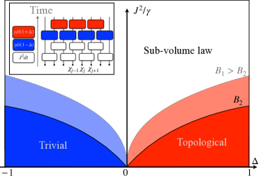
Figure 1: Schematic drawing of the phase diagram for the model in the inset under partial post-selection. Under strong partial post-selection, reducing the degree of post-selection B1>B2𝐵1subscript𝐵2B1>B_{2}, leads to an expansion of the sub-volume law phase. Inset: quantum circuit representation of the model consisting of random unitary evolution (white) and competing sets of parity measurements (blue and red) of Majorana fermions.

MiPTs in the post-selected limit of monitored dynamics exhibit key differences compared to their monitored counterparts. These differences extend from features of the phase diagram to the universality class of the transition [10, 52]. There have been some steps to incorporate sparse quantum jumps beyond the post-selected limit [54, 56] or to map the full crossover explored numerically [10], however, a theory that captures a systematic way to include a fraction of trajectories and explains the change in MiPTs properties is generally lacking. This is the question we address in this paper. We first summarize here our main findings.

We derive a partial-post-selected (PPS) stochastic Schrödinger equation (SSE) — cf. Eq.(I), with a continuous parameter B𝐵B that controls the range of detector’s outcomes that are retained. The PPS-SSE includes the fully monitored and fully post-selected dynamics as limiting cases and is valid for a generic quantum system with a continuously monitored Hermitian observable.

Next, we apply our analytic PPS approach to study the MiPT driven by non-commuting sets of local parity measurements in a real free fermionic chain. In this model, the post-selected dynamics feature an area-to-area topological MiPT driven by the competing measurements, with a different critical exponent than its monitored analogue [10]. Using the PPS-SSE approach and within a 2-replica approximation, we obtain an effective description of the steady-state out-of-equilibrium phases in terms of an effective Hamiltonian—cf. Eqs. (31,V,IV). From a Renormalization Group (RG) flow analysis, we find that the post-selected universal properties of the MiPT persist when one moves away from the post-selected limit by increasing the range of outcomes retained —cf. Sec. VI.1, Fig. 4.

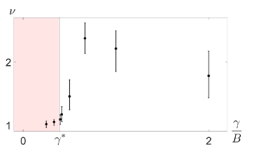
Our calculation further shows that the Luttinger parameter of the effective bosonized theory for strong post-selection diverges at a finite value of partial post-selection,B𝐵B, which may indicate a phase transition driven by the stochasticity from quantum trajectories. This result is supported by numerical calculation which identifies non-monotonic behavior of the critical exponent at similar values of B𝐵B —cf. Fig. 5.

In the presence of unitary dynamics, the partial post-selected model features two distinct area law phases separated by a sub-volume law phase. We find that the sub-volume phase becomes increasingly stable upon moving away from the post-selected limit, as shown in Fig. 1 —cf. Sec. VI.2, Fig. 7.

The rest of the paper is structured as follows. We develop the formalism of partial post-selection in Sec. I and extend it to the replica formalism in Sec. II. Sec. III presents the model of interest, with the corresponding effective 2-replica description in Sec. IV and the effective theory for the strong-post-selection regime in Sec. V. The results are presented in Sec. VI with a final discussion and conclusions in Sec. VII. Throughout this paper, we shall use the terms ‘post-selected’ and ‘monitored’ to indicate respectively the fully post-selected measurement dynamics and the fully stochastic continuous measurement where all readouts are retained respectively.

I partial post-selection

We consider the dynamics of a continuously monitored quantum system whose evolution is described by the stochastic Schrödinger equation (SSE)

d|ψt=𝑑ketsubscript𝜓𝑡absent\displaystyle d\mathinner{|{\psi_{t}}\rangle}= [idtHdtγ2j(O^jO^j)2\displaystyle\left[-idtH-dt\frac{\gamma}{2}\sum_{j}\left(\hat{O}_{j}-\langle\hat{O}_{j}\rangle\right)^{2}\right.
+jdWj(O^jO^j)]|ψt,\displaystyle\left.+\sum_{j}dW_{j}\left(\hat{O}_{j}-\langle\hat{O}_{j}\rangle\right)\right]\mathinner{|{\psi_{t}}\rangle}, (1)

where |ψtketsubscript𝜓𝑡\mathinner{|{\psi_{t}}\rangle} is the system’s state at time t𝑡t, O^jsubscript^𝑂𝑗\hat{O}_{j} the set of observables being measured, and H𝐻H the system’s Hamiltonian. To lighten the notation, we shall drop the hat above the measurement operator unless it is needed for clarity. Eq. (I) is the Ito formulation of stochastic dynamics with dWj𝑑subscript𝑊𝑗dW_{j} uncorrelated Gaussian-distributed stochastic increments with dWjdWk¯=γdtδj,k¯𝑑subscript𝑊𝑗𝑑subscript𝑊𝑘𝛾𝑑𝑡subscript𝛿𝑗𝑘\overline{dW_{j}dW_{k}}=\gamma dt\delta_{j,k}, where γ𝛾\gamma is the inverse measurement time at which typical stochastic realizations of the quantum trajectories are close to the observable’s eigenvalue.
Refer to caption
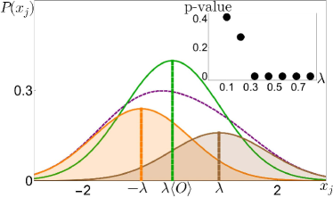
Figure 2: Probability distribution of continuous Gaussian measurement readouts (3). The readout distribution P(xj)𝑃subscript𝑥𝑗P(x_{j}) (dashed purple) results from the sum of two overlapping Gaussians (brown and orange shaded), centred at positions λ𝜆\lambda and λ𝜆-\lambda with different heights Πj,delimited-⟨⟩subscriptΠ𝑗\langle\Pi_{j,-}\rangle and Πj,+delimited-⟨⟩subscriptΠ𝑗\langle\Pi_{j,+}\rangle respectively. P(xj)𝑃subscript𝑥𝑗P(x_{j}) is approximated by the Gaussian distribution (green) in Eq. (3) which becomes exact in the limit of continuous measurements — cf. inset. Inset: Accuracy of the approximation in Eq.(3) quantified via a two-sample Kolmogorov-Smirnov test [64]. The accuracy (p-value) increases with decreasing λ𝜆\lambda, and becomes exact in the case of continuous measurement λdt0similar-to𝜆𝑑𝑡0\lambda\sim\sqrt{dt}\to 0. The parameters are set as λ=0.8𝜆0.8\lambda=0.8, Πj,+=0.4delimited-⟨⟩subscriptΠ𝑗0.4\langle\Pi_{j,+}\rangle=0.4 and Πj,=0.6delimited-⟨⟩subscriptΠ𝑗0.6\langle\Pi_{j,-}\rangle=0.6.

To develop the idea of partial post-selection, we start with a microscopic model of the measurement process leading to the SSE. We consider the measurement process described by a positively valued measurement [51]. In this case, after coupling the detector to the system in a state |ψtsubscriptket𝜓𝑡\mathinner{|{\psi}\rangle}_{t}, the process returns a readout xjsubscript𝑥𝑗x_{j}, drawn from a probability distribution P(xj)=ψt|Kj(xj)Kj(xj)|ψt𝑃subscript𝑥𝑗brasubscript𝜓𝑡subscript𝐾𝑗superscriptsubscript𝑥𝑗subscript𝐾𝑗subscript𝑥𝑗ketsubscript𝜓𝑡P(x_{j})=\mathinner{\langle{\psi_{t}}|}K_{j}(x_{j})^{\dagger}K_{j}(x_{j})\mathinner{|{\psi_{t}}\rangle}, and a conditional state update |ψt+dt=Kj(xj)|ψt/P(xj)ketsubscript𝜓𝑡𝑑𝑡subscript𝐾𝑗subscript𝑥𝑗ketsubscript𝜓𝑡𝑃subscript𝑥𝑗\mathinner{|{\psi_{t+dt}}\rangle}=K_{j}(x_{j})\mathinner{|{\psi_{t}}\rangle}/\sqrt{P(x_{j})}. The process is entirely dictated by the Kraus operators Kj(xj)subscript𝐾𝑗subscript𝑥𝑗K_{j}(x_{j}).

We consider here specifically the case of continuously monitoring an observable Ojsubscript𝑂𝑗O_{j} as performed by a pointer with a continuous readout xjsubscript𝑥𝑗x_{j} with Gaussian a-priori distribution G(x)=1/2πΔ2exp(x2/2Δ2)𝐺𝑥12𝜋superscriptΔ2superscript𝑥22superscriptΔ2G(x)=1/\sqrt{2\pi\Delta^{2}}\exp(-x^{2}/2\Delta^{2}). We further restrict to the simplest case of a measurement operator O^j=Π^j,+Π^j,subscript^𝑂𝑗subscript^Π𝑗subscript^Π𝑗\hat{O}_{j}=\hat{\Pi}_{j,+}-\hat{\Pi}_{j,-} which acts in the 2-dimensional space with projector Π^+/subscript^Πabsent\hat{\Pi}_{+/-} and squares to identity O^j2=𝕀superscriptsubscript^𝑂𝑗2𝕀\hat{O}_{j}^{2}=\mathbb{I}. The Kraus operators are then given by [51]

Kj(xj,λ)=G(xjλ)Πj,++G(xj+λ)Πj,,subscript𝐾𝑗subscript𝑥𝑗𝜆𝐺subscript𝑥𝑗𝜆subscriptΠ𝑗𝐺subscript𝑥𝑗𝜆subscriptΠ𝑗K_{j}(x_{j},\lambda)=\sqrt{G(x_{j}-\lambda)}\Pi_{j,+}+\sqrt{G(x_{j}+\lambda)}\Pi_{j,-}, (2)

and

P(xj)=G(xλ)Πj,++G(x+λ)Πj,.𝑃subscript𝑥𝑗𝐺𝑥𝜆delimited-⟨⟩subscriptΠ𝑗𝐺𝑥𝜆delimited-⟨⟩subscriptΠ𝑗P(x_{j})=G(x-\lambda)\langle\Pi_{j,+}\rangle+G(x+\lambda)\langle\Pi_{j,-}\rangle. (3)

The continuous SSE in Eq. (I) is recovered by setting λ2=γdtsuperscript𝜆2𝛾𝑑𝑡\lambda^{2}=\gamma dt, where dt0𝑑𝑡0dt\to 0 with γ𝛾\gamma finite guarantees λ1much-less-than𝜆1\lambda\ll 1. In this limit,

P(xj)𝑃subscript𝑥𝑗\displaystyle P(x_{j}) 12πΔ2exp((xjλOj)22Δ2),absent12𝜋superscriptΔ2superscriptsubscript𝑥𝑗𝜆delimited-⟨⟩subscript𝑂𝑗22superscriptΔ2\displaystyle\approx\frac{1}{\sqrt{2\pi\Delta^{2}}}\exp(-\frac{(x_{j}-\lambda\langle O_{j}\rangle)^{2}}{2\Delta^{2}}),
Kj(xj,λ)subscript𝐾𝑗subscript𝑥𝑗𝜆\displaystyle K_{j}(x_{j},\lambda) 1(2πΔ2)1/4exp((xjλOj)24Δ2).absent1superscript2𝜋superscriptΔ214superscriptsubscript𝑥𝑗𝜆subscript𝑂𝑗24superscriptΔ2\displaystyle\approx\frac{1}{(2\pi\Delta^{2})^{1/4}}\exp(-\frac{(x_{j}-\lambda O_{j})^{2}}{4\Delta^{2}}). (4)

The probability distribution is schematically shown in figure (2). Notably, in eq. I, we have used the fact that in the continuum limit λ2=γdt0superscript𝜆2𝛾𝑑𝑡0\lambda^{2}=\gamma dt\to 0, Δ𝒪(dt0)similar-toΔ𝒪𝑑superscript𝑡0\Delta\sim\mathcal{O}(dt^{0}).

The scenario of multiple measurement events can be written readily down: if there are L𝐿L lots of measurement operators O^j,j[1L]subscript^𝑂𝑗𝑗delimited-[]1𝐿\hat{O}_{j},j\in[1\dots L], the final state after measurements across all operators is

|ψt+dt=1𝒩j=1LKj(xj,λ)|ψt,ketsubscript𝜓𝑡𝑑𝑡1𝒩superscriptsubscriptproduct𝑗1𝐿subscript𝐾𝑗subscript𝑥𝑗𝜆ketsubscript𝜓𝑡\displaystyle\mathinner{|{\psi_{t+dt}}\rangle}=\frac{1}{\mathcal{N}}\prod_{j=1}^{L}K_{j}(x_{j},\lambda)\mathinner{|{\psi_{t}}\rangle}, (5)

where the results hold in the continuum limit dt0𝑑𝑡0dt\to 0 to order 𝒪(dt)𝒪𝑑𝑡\mathcal{O}(dt) also if some of the operators 𝒪jsubscript𝒪𝑗\mathcal{O}_{j} do not commute. As a side note, (2) can also be generalised to measurement operators with arbitrary spectrum with the same procedure illustrated above [51].

The process of post-selection amounts to choosing and retaining the quantum trajectories that correspond to a unique set of predetermined detector readouts {xj}subscript𝑥𝑗\{x_{j}\}, while discarding the rest. We generalize this procedure to achieve Partial Post-Selection (PPS) by retaining all quantum trajectories that correspond to a finite range of detector outcomes. A natural means to achieve PPS is to force some degree of bias in the measurement outcome retaining the detector’s outcome only if they are larger than a given, preset value, rcsubscript𝑟𝑐r_{c}. This amounts to truncating the readout probability distribution function P(xj)𝑃subscript𝑥𝑗P(x_{j}) to a modified one,

Prc(xj)=P(xj)Θ(xjrc)e(xjλOjδλ)22(Δ+δ)2P¯(xj),subscript𝑃subscript𝑟𝑐subscript𝑥𝑗𝑃subscript𝑥𝑗Θsubscript𝑥𝑗subscript𝑟𝑐superscript𝑒superscriptsubscript𝑥𝑗𝜆delimited-⟨⟩subscript𝑂𝑗𝛿𝜆22superscriptΔ𝛿2¯𝑃subscript𝑥𝑗\displaystyle P_{r_{c}}(x_{j})=P(x_{j})\Theta(x_{j}-r_{c})\approx e^{-\frac{(x_{j}-\lambda\langle O_{j}\rangle-\delta\lambda)^{2}}{2(\Delta+\delta)^{2}}}\equiv\underline{P}(x_{j}), (6)

where Θ(x)Θ𝑥\Theta(x) is the Heaviside step function.

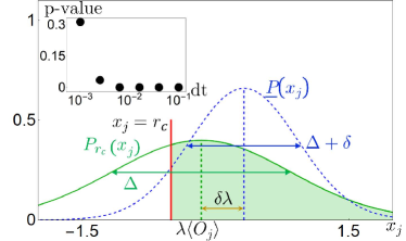
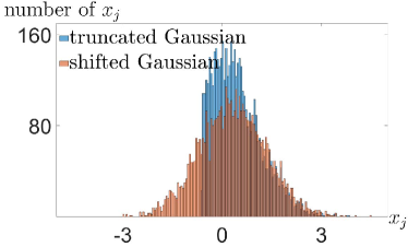
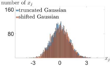
In the last step in Eq. (6), we have approximated the truncated distribution by a Gaussian distribution whose mean and variance, parametrised by δλ𝛿𝜆\delta\lambda and δ𝛿\delta respectively, are determined by demanding that they coincide with those of Prc(xj)subscript𝑃subscript𝑟𝑐subscript𝑥𝑗P_{r_{c}}(x_{j}), as illustrated in Fig. (3). While the distribution Prcsubscript𝑃subscript𝑟𝑐P_{r_{c}} and P¯¯𝑃\underline{P} are generically different, we demand a proper scaling of rcsubscript𝑟𝑐r_{c} with dt0𝑑𝑡0dt\to 0, so that the two distributions coincide in the continuum limit. This is achieved with the scaling

δλ=bλ=bγdt,𝛿𝜆𝑏𝜆𝑏𝛾𝑑𝑡\displaystyle\delta\lambda=b\lambda=b\sqrt{\gamma dt}, (7)

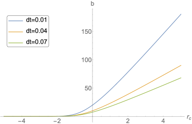
where b𝑏b is kept constant in the limit dt0𝑑𝑡0dt\to 0 (see Appendix A). The relation between rcsubscript𝑟𝑐r_{c} and b𝑏b is derived and discussed in Appendix A, and b𝑏b captures the discrete-time process rcsubscript𝑟𝑐r_{c} in the time continuum limit, in analogy to γ𝛾\gamma capturing the discrete process λ𝜆\lambda in continuous measurement backaction. On the other hand, the correction in variance, δ𝛿\delta, can be safely ignored (Appendix A). Importantly, at leading order in dt𝑑𝑡dt, the functional dependence of rcsubscript𝑟𝑐r_{c} on b𝑏b is independent of the system’s state, so that the continuum limit at constant b𝑏b corresponds to an operationally well-defined truncation of the probability P(xj)𝑃subscript𝑥𝑗P(x_{j}).

Refer to caption
Figure 3: Partial-post selection procedure in (6). The measurement outcome Gaussian distribution (green) is truncated at xj=rcsubscript𝑥𝑗subscript𝑟𝑐x_{j}=r_{c}, resulting in a new distribution Prc(xj)subscript𝑃subscript𝑟𝑐subscript𝑥𝑗P_{r_{c}}(x_{j}) (shaded) with shifted mean λλ+δλ𝜆𝜆𝛿𝜆\lambda\rightarrow\lambda+\delta\lambda and shifted variance Δ2(Δ+δ)2superscriptΔ2superscriptΔ𝛿2\Delta^{2}\rightarrow(\Delta+\delta)^{2}. Prcsubscript𝑃subscript𝑟𝑐P_{r_{c}} is approximated by a new Gaussian, P¯(xj)¯𝑃subscript𝑥𝑗\underline{P}(x_{j}) (blue), with mean λ+δλ𝜆𝛿𝜆\lambda+\delta\lambda and variance (Δ+δ)2superscriptΔ𝛿2(\Delta+\delta)^{2}. The approximation is valid in the continuum limit as shown in the inset. Inset: p-value from a KS2 test for the two distributions Prcsubscript𝑃subscript𝑟𝑐P_{r_{c}} and P¯¯𝑃\underline{P} with various dt𝑑𝑡dt. The approximation is exact in the continuum limit dt0𝑑𝑡0dt\to 0 The parameters are set as Oj=0.2,rc=0.5formulae-sequencedelimited-⟨⟩subscript𝑂𝑗0.2subscript𝑟𝑐0.5\langle O_{j}\rangle=0.2,\ r_{c}=-0.5 and λ=0.3𝜆0.3\lambda=0.3.

We show explicitly via a two-sample Kolmogorov-Smirnov (KS2) test from a numerical sampling of Prcsubscript𝑃subscript𝑟𝑐P_{r_{c}} and P¯¯𝑃\underline{P} [64], that the approximation by a Gaussian distribution in the time continuum analysis becomes exact in the continuum limit. The results are reported in figure 3, with the inset showing that the p-values (a statistical measure of overlap) of the two distributions are increasing with small time increments dt𝑑𝑡dt.

The continuum limit of P¯(xj)¯𝑃subscript𝑥𝑗\underline{P}(x_{j}) in Eq. (6), allows us to obtain a corresponding PPS SSE. Specifically, we introduce a new random variable ξj=xj/ΔλOjbλ,mean(ξj)=0,Var(ξj)=1formulae-sequencesubscript𝜉𝑗subscript𝑥𝑗Δ𝜆delimited-⟨⟩subscript𝑂𝑗𝑏𝜆formulae-sequencemeansubscript𝜉𝑗0Varsubscript𝜉𝑗1\xi_{j}=x_{j}/\Delta-\lambda\langle O_{j}\rangle-b\lambda\ ,\ \textbf{mean}(\xi_{j})=0,\textbf{Var}(\xi_{j})=1. When expressed in terms of ξ𝜉\xi, the update of the state by the Kraus operator in (5) becomes

|ψt+dtketsubscript𝜓𝑡𝑑𝑡\displaystyle\mathinner{|{\psi_{t+dt}}\rangle} =1𝒩jKj(xj,λ)|ψtabsent1𝒩subscriptproduct𝑗subscript𝐾𝑗subscript𝑥𝑗𝜆ketsubscript𝜓𝑡\displaystyle=\frac{1}{\mathcal{N}}\prod_{j}K_{j}(x_{j},\lambda)\mathinner{|{\psi_{t}}\rangle}
=1𝒩2je(λ2(OjOjb)24Δ2+ξjλOjOjb2Δ)|ψt,absent1subscript𝒩2subscriptproduct𝑗superscript𝑒superscript𝜆2superscriptsubscript𝑂𝑗delimited-⟨⟩subscript𝑂𝑗𝑏24superscriptΔ2subscript𝜉𝑗𝜆subscript𝑂𝑗delimited-⟨⟩subscript𝑂𝑗𝑏2Δketsubscript𝜓𝑡\displaystyle=\frac{1}{\mathcal{N}_{2}}\prod_{j}e^{\left(\frac{\lambda^{2}(O_{j}-\langle O_{j}\rangle-b)^{2}}{4\Delta^{2}}+\xi_{j}\lambda\frac{O_{j}-\langle O_{j}\rangle-b}{2\Delta}\right)}\mathinner{|{\psi_{t}}\rangle}, (8)

where overall factors have been reabsorbed in the state-normalization 𝒩2subscript𝒩2\mathcal{N}_{2}. By setting Δ=1/2Δ12\Delta=1/2, λ2=γdtsuperscript𝜆2𝛾𝑑𝑡\lambda^{2}=\gamma dt and noticing that the random variable ξjγdt=dWjsubscript𝜉𝑗𝛾𝑑𝑡𝑑subscript𝑊𝑗\xi_{j}\sqrt{\gamma dt}=dW_{j} fulfils dWjdWk¯=γdt¯𝑑subscript𝑊𝑗𝑑subscript𝑊𝑘𝛾𝑑𝑡\overline{dW_{j}dW_{k}}=\gamma dt, the state update in Eq. (I) defines a Wiener process to order dt𝑑𝑡dt and we arrive at the modified partial-post selected stochastic Schrödinger equation (PPS SSE)

d|ψt=idtH|ψtdtγ2j(O^jO^j)2|ψt𝑑ketsubscript𝜓𝑡𝑖𝑑𝑡𝐻ketsubscript𝜓𝑡𝑑𝑡𝛾2subscript𝑗superscriptsubscript^𝑂𝑗delimited-⟨⟩subscript^𝑂𝑗2ketsubscript𝜓𝑡\displaystyle d\mathinner{|{\psi_{t}}\rangle}=-idtH\mathinner{|{\psi_{t}}\rangle}-dt\frac{\gamma}{2}\sum_{j}\left(\hat{O}_{j}-\langle\hat{O}_{j}\rangle\right)^{2}\mathinner{|{\psi_{t}}\rangle}
+Bdtj(O^jO^j)|ψt+jdWj(O^jO^j)|ψt,𝐵𝑑𝑡subscript𝑗subscript^𝑂𝑗delimited-⟨⟩subscript^𝑂𝑗ketsubscript𝜓𝑡subscript𝑗𝑑subscript𝑊𝑗subscript^𝑂𝑗delimited-⟨⟩subscript^𝑂𝑗ketsubscript𝜓𝑡\displaystyle+Bdt\sum_{j}\left(\hat{O}_{j}-\langle\hat{O}_{j}\rangle\right)\mathinner{|{\psi_{t}}\rangle}+\sum_{j}dW_{j}\left(\hat{O}_{j}-\langle\hat{O}_{j}\rangle\right)\mathinner{|{\psi_{t}}\rangle}, (9)

where we set B=bγ𝐵𝑏𝛾B=b\gamma and dWjdWk=γdtδj,k𝑑subscript𝑊𝑗𝑑subscript𝑊𝑘𝛾𝑑𝑡subscript𝛿𝑗𝑘dW_{j}dW_{k}=\gamma dt\delta_{j,k}. Eq. (I) is the first main result of our work. It generalises the SSE for observables of a 2-dimensional Hilbert space to account for a partial selection of trajectories defined in an operationally meaningful procedure. From, Eq. (I), we can clearly identify two limits: for γ0𝛾0\gamma\neq 0, B=0𝐵0B=0 we recover the standards SSE for monitored dynamics, while for γ=0𝛾0\gamma=0, B0𝐵0B\neq 0 we are in the post-selected limit governed by a non-Hermitian Hamiltonian Heff=H+iBjO^jsubscript𝐻eff𝐻𝑖𝐵subscript𝑗subscript^𝑂𝑗H_{\text{eff}}=H+iB\sum_{j}\hat{O}_{j}. We also note that the sign of the non-Hermitian term can be flipped by simply defining rcsubscript𝑟𝑐r_{c} from the positive side of xjsubscript𝑥𝑗x_{j}. Note that the post-selected limit is operationally obtained by γ0𝛾0\gamma\to 0 but b1/γproportional-to𝑏1𝛾b\propto 1/\gamma with γb=const𝛾𝑏const\gamma b=\textrm{const}.

II Measurement induced transition and replicated dynamics

The effect of partial post-selection can equivalently be captured in the evolution of the system density matrix. If we consider a density matrix evolved along a quantum trajectory with a certain set of measurement outcomes {xt},t[1M]subscript𝑥𝑡𝑡delimited-[]1𝑀\{x_{t}\},t\in[1...M] is a discrete-time index. The resultant density matrix is given by

ρ{xt}=ρˇ{xt}Tr[ρˇ{xt}],subscript𝜌subscript𝑥𝑡subscriptˇ𝜌subscript𝑥𝑡tracesubscriptˇ𝜌subscript𝑥𝑡\displaystyle\rho_{\{x_{t}\}}=\frac{\check{\rho}_{\{x_{t}\}}}{\Tr[\check{\rho}_{\{x_{t}\}}]}, (10)

where ρˇ{xt}=KxMKx2Kx1ρ0Kx1Kx2KxMsubscriptˇ𝜌subscript𝑥𝑡subscript𝐾subscript𝑥𝑀subscript𝐾subscript𝑥2subscript𝐾subscript𝑥1subscript𝜌0subscriptsuperscript𝐾subscript𝑥1subscriptsuperscript𝐾subscript𝑥2subscriptsuperscript𝐾subscript𝑥𝑀\check{\rho}_{\{x_{t}\}}=K_{x_{M}}\dots K_{x_{2}}K_{x_{1}}\rho_{0}K^{\dagger}_{x_{1}}K^{\dagger}_{x_{2}}\dots K^{\dagger}_{x_{M}} is the the un-normalised density matrix along the trajectory, Kxlsubscript𝐾subscript𝑥𝑙K_{x_{l}} the Kraus operator in Eq. (2) is associated with measurement outcome xlsubscript𝑥𝑙x_{l} and ρ0subscript𝜌0\rho_{0} is the initial normalised density matrix. From here onward, we will specify an un-normalised density matrix by a caron above: ρ=ρˇ/Tr[ρˇ]𝜌ˇ𝜌traceˇ𝜌\rho=\check{\rho}/\Tr[\check{\rho}].

Since the probability of this trajectory, labelled by {xt}subscript𝑥𝑡\{x_{t}\}, is P({xt})=Tr[ρˇ{xt}]𝑃subscript𝑥𝑡Trdelimited-[]subscriptˇ𝜌subscript𝑥𝑡P(\{x_{t}\})=\text{Tr}[\check{\rho}_{\{x_{t}\}}], the average density matrix over all trajectories is

ρ¯={xt}ρˇ{xt}Tr[ρˇ{xt}]P({xt})={xt}ρˇ{xt},¯𝜌subscriptsubscript𝑥𝑡subscriptˇ𝜌subscript𝑥𝑡Trdelimited-[]subscriptˇ𝜌subscript𝑥𝑡𝑃subscript𝑥𝑡subscriptsubscript𝑥𝑡subscriptˇ𝜌subscript𝑥𝑡\displaystyle\overline{\rho}=\sum_{\{x_{t}\}}\frac{\check{\rho}_{\{x_{t}\}}}{\text{Tr}[\check{\rho}_{\{x_{t}\}}]}P(\{x_{t}\})=\sum_{\{x_{t}\}}\check{\rho}_{\{x_{t}\}}, (11)

where we use ¯¯\overline{\cdot} to indicate the average over quantum trajectories and the sum runs over all possible set of measurement outcome. In the continuum limit, the evolution of ρ¯¯𝜌\overline{\rho} is governed by a Lindblad equation, which, in the typical cases of incompatible measurements and/or unitary dynamics considered here admits as a long-term fixed point the maximally mixed state limtρ¯t𝕀similar-tosubscript𝑡subscript¯𝜌𝑡𝕀\lim_{t\to\infty}\overline{\rho}_{t}\sim\mathbb{I}.

To capture non-trivial effects from measurements in the steady-state ensemble of quantum trajectories, one, therefore, needs to consider the evolution along individual trajectories, i.e. via post-selection, or resort to averages of quantities which are non-linear in density matrix e.g.O^k¯=Tr[O^ρ]k¯\overline{\langle\hat{O}\rangle^{k}}=\overline{\Tr[\hat{O}\rho]^{k}}, or the k𝑘k-th Renyì entropy Sk¯=1/(1k)log(Tr[ρk])¯subscript𝑆𝑘11𝑘tracesuperscript𝜌𝑘\overline{S_{k}}=1/(1-k)\log\left(\Tr[\rho^{k}]\right), k>1𝑘1k>1.

To treat analytically these non-linear averages one can resort to a powerful mathematical construction, the replica trick [65, 18, 9, 66], where one considers identical replicas of the system’s density matrix. The average of the replicated density matrix can then be related to the average of the non-linear quantities we are interested in. In fact,

Ok¯¯superscriptdelimited-⟨⟩𝑂𝑘\displaystyle\overline{\langle O\rangle^{k}} ={xt}(Tr[Oρ{xt}])kP({xt})absentsubscriptsubscript𝑥𝑡superscriptTrdelimited-[]𝑂subscript𝜌subscript𝑥𝑡𝑘𝑃subscript𝑥𝑡\displaystyle=\sum_{\{x_{t}\}}\left(\text{Tr}[O\rho_{\{x_{t}\}}]\right)^{k}P(\{x_{t}\})
={xt}Tr[Okρˇ{xt}k](Tr[ρˇ{xt}])1kabsentsubscriptsubscript𝑥𝑡Trdelimited-[]superscript𝑂tensor-productabsent𝑘subscriptsuperscriptˇ𝜌tensor-productabsent𝑘subscript𝑥𝑡superscriptTrdelimited-[]subscriptˇ𝜌subscript𝑥𝑡1𝑘\displaystyle=\sum_{\{x_{t}\}}\text{Tr}[O^{\otimes k}\check{\rho}^{\otimes k}_{\{x_{t}\}}](\text{Tr}[\check{\rho}_{\{x_{t}\}}])^{1-k}
=limn1{xt}Tr[(Ok𝕀nk)ρˇ{xt}n],absentsubscript𝑛1subscriptsubscript𝑥𝑡tracetensor-productsuperscript𝑂tensor-productabsent𝑘superscript𝕀tensor-productabsent𝑛𝑘subscriptsuperscriptˇ𝜌tensor-productabsent𝑛subscript𝑥𝑡\displaystyle=\lim\limits_{n\to 1}\sum_{\{x_{t}\}}\Tr\left[\left(O^{\otimes k}\otimes\mathbb{I}^{\otimes n-k}\right)\check{\rho}^{\otimes n}_{\{x_{t}\}}\right], (12)

and the non-linear quantity encoding the non-trivial effects of measurement-induced dynamics is the trajectories averaged n𝑛n-replicated un-normalised density matrix {xt}ρˇ{xt}n=ρˇn¯,nkformulae-sequencesubscriptsubscript𝑥𝑡subscriptsuperscriptˇ𝜌tensor-productabsent𝑛subscript𝑥𝑡¯superscriptˇ𝜌tensor-productabsent𝑛𝑛𝑘\sum_{\{x_{t}\}}\check{\rho}^{\otimes n}_{\{x_{t}\}}=\overline{\check{\rho}^{\otimes n}},n\geq k. Eq. (II) shows that the fundamental object of interest is ρˇn¯¯superscriptˇ𝜌tensor-productabsent𝑛\overline{\check{\rho}^{\otimes n}}, and the limit n1𝑛1n\rightarrow 1 is an analytical continuation for k>1𝑘1k>1. Importantly, the replica limit here is taken as n1𝑛1n\rightarrow 1, which poses a different case from the standard limit n0𝑛0n\rightarrow 0 resulting from the replica trick for disordered systems [67, 68].

Since the entanglement between two subsystems is determined by the purity of one of them, the simplest MiPT in the entanglement properties of the system can be identified by the k𝑘k-th purity of a subsystem. The k𝑘k-th purity μk,𝐀=Tr[ρ𝐀k]subscript𝜇𝑘𝐀tracesuperscriptsubscript𝜌𝐀𝑘\mu_{k,\mathbf{A}}=\Tr[\rho_{\mathbf{A}}^{k}] of a subsystem 𝐀𝐀\mathbf{A} involves the k𝑘k-th power of the reduced density matrix and can be calculated using the replica trick by introducing a suitable operator in the replica space, 𝒞k,𝐀subscript𝒞𝑘𝐀\mathcal{C}_{k,\mathbf{A}}, as [65, 18]

μk,𝐀=Tr[ρ𝐀k]=Tr[𝒞k,𝐀ρk],subscript𝜇𝑘𝐀tracesuperscriptsubscript𝜌𝐀𝑘tracesubscript𝒞𝑘𝐀superscript𝜌tensor-productabsent𝑘\displaystyle\mu_{k,\mathbf{A}}=\Tr[\rho_{\mathbf{A}}^{k}]=\Tr[\mathcal{C}_{k,\mathbf{A}}\rho^{\otimes k}], (13)

where ρ𝜌\rho is the normalised density matrix and

𝒞k,𝐀=𝐀jj=1j=k|𝐀j𝐀j+1|,subscript𝒞𝑘𝐀subscriptsubscript𝐀𝑗subscriptsuperscripttensor-product𝑗𝑘𝑗1ketsubscript𝐀𝑗brasubscript𝐀𝑗1\mathcal{C}_{k,\mathbf{A}}=\sum_{\mathbf{A}_{j}}\bigotimes^{j=k}_{j=1}\mathinner{|{\mathbf{A}_{j}}\rangle}\mathinner{\langle{\mathbf{A}_{j+1}}|}, (14)

and the sum indicates that |𝐀j,(j mod k)ketsubscript𝐀𝑗j mod k\mathinner{|{\mathbf{A}_{j}}\rangle},\ (\text{j mod k}) runs over all the basis in the subsystem 𝐀𝐀\mathbf{A}. Note that 𝒞k,𝐀subscript𝒞𝑘𝐀\mathcal{C}_{k,\mathbf{A}} acts as an identity outside of 𝐀𝐀\mathbf{A} while cyclically permutes kets from k𝑘k replicated density matrix in 𝐀𝐀\mathbf{A}. The associated k𝑘k-th Rényi entropy Sk,𝐀subscript𝑆𝑘𝐀S_{k,\mathbf{A}}, which is an entanglement measure, is related by Sk,𝐀=1/(1k)logμk,𝐀subscript𝑆𝑘𝐀11𝑘subscript𝜇𝑘𝐀S_{k,\mathbf{A}}=1/(1-k)\log\mu_{k,\mathbf{A}}.

Throughout most of this paper, we focus on the 2-replica analysis and replace the true replica limit n1𝑛1n\rightarrow 1 by n=2𝑛2n=2. This 2-replica approximation captures non-trivial measurement-induced effect, includes information about the true replica limit, and hence provides a valid figure of merit to identify the non-trivial effects of PPS on measurement-induced dynamics [66, 65]. The 222-replica approximation allows one to access distorted average of quantities with a quadratic dependence on the density matrix [66, 65], i.e. k,n=2𝑘𝑛2k,n=2 in Eq. (II) as

{xt}Tr[O2ρˇ{xt}2]{xt}Tr[ρˇ{xt}2]={xt}P({xt})2Tr[Oρxt]2{xt}P({xt})2=O2¯¯subscriptsubscript𝑥𝑡Trdelimited-[]superscript𝑂tensor-productabsent2subscriptsuperscriptˇ𝜌tensor-productabsent2subscript𝑥𝑡subscriptsubscript𝑥𝑡tracesubscriptsuperscriptˇ𝜌tensor-productabsent2subscript𝑥𝑡subscriptsubscript𝑥𝑡𝑃superscriptsubscript𝑥𝑡2Trsuperscriptdelimited-[]𝑂subscript𝜌subscript𝑥𝑡2subscriptsubscript𝑥𝑡𝑃superscriptsubscript𝑥𝑡2¯¯superscriptdelimited-⟨⟩𝑂2\displaystyle\frac{\sum_{\{x_{t}\}}\text{Tr}[O^{\otimes 2}\check{\rho}^{\otimes 2}_{\{x_{t}\}}]}{\sum_{\{x_{t}\}}\Tr[\check{\rho}^{\otimes 2}_{\{x_{t}\}}]}=\frac{\sum_{\{x_{t}\}}P(\{x_{t}\})^{2}\text{Tr}[O\rho_{x_{t}}]^{2}}{\sum_{\{x_{t}\}}P(\{x_{t}\})^{2}}=\overline{\overline{\langle O\rangle^{2}}} (15)

where the denominator is included for normalization. Eq. (15) shows that the approximation corresponds indeed to averaging with a distorted probability distribution, now given by P({xt})2𝑃superscriptsubscript𝑥𝑡2P(\{x_{t}\})^{2}, and we denote this by a double over line above, ¯¯¯¯\overline{\overline{\cdot}}.

Within this approximation, the distorted 222-nd purity μ¯¯2,𝐀subscript¯¯𝜇2𝐀\overline{\overline{\mu}}_{2,\mathbf{A}} can be calculated using the operator in (14) as:

μ¯¯2,𝐀=Tr[𝒞k,𝐀{xt}ρˇ{xt}2]Tr[{xt}ρˇ{xt}2],subscript¯¯𝜇2𝐀tracesubscript𝒞𝑘𝐀subscriptsubscript𝑥𝑡superscriptsubscriptˇ𝜌subscript𝑥𝑡tensor-productabsent2tracesubscriptsubscript𝑥𝑡superscriptsubscriptˇ𝜌subscript𝑥𝑡tensor-productabsent2\displaystyle\overline{\overline{\mu}}_{2,\mathbf{A}}=\frac{\Tr[\mathcal{C}_{k,\mathbf{A}}\sum_{\{x_{t}\}}\check{\rho}_{\{x_{t}\}}^{\otimes 2}]}{\Tr[\sum_{\{x_{t}\}}\check{\rho}_{\{x_{t}\}}^{\otimes 2}]}, (16)

and the associated conditional 222-nd Rényi entropy Sk,𝐀(cond)=logμ¯¯k,𝐀superscriptsubscript𝑆𝑘𝐀condsubscript¯¯𝜇𝑘𝐀S_{k,\mathbf{A}}^{(\text{cond})}=-\log\overline{\overline{\mu}}_{k,\mathbf{A}} is an entanglement measure of an extended system including both the system and the detector [65, 66]. Thus, the trajectories averaged 2-replica {xt}ρˇ{xt}2subscriptsubscript𝑥𝑡subscriptsuperscriptˇ𝜌tensor-productabsent2subscript𝑥𝑡\sum_{\{x_{t}\}}\check{\rho}^{\otimes 2}_{\{x_{t}\}} shall capture MiPT in the system.

We also note that the calculation of entanglement entropy S0,𝐀Tr[ρ𝐀logρ𝐀]subscript𝑆0𝐀tracesubscript𝜌𝐀subscript𝜌𝐀S_{0,\mathbf{A}}\equiv\Tr[\rho_{\mathbf{A}}\log\rho_{\mathbf{A}}] for Gaussian fermions, at leading order, amounts to taking k=2𝑘2k=2 in (II[69, 20, 9]. Therefore in leading order, the 2-replica approximation is expected to retain some information about the true replica limit entanglement entropy.

In Sec. IV, we will show that the characterisation of the fundamental object in this 2 replica approximation limt{xt}ρˇ{xt}2subscript𝑡subscriptsubscript𝑥𝑡subscriptsuperscriptˇ𝜌tensor-productabsent2subscript𝑥𝑡\lim\limits_{t\to\infty}\sum_{\{x_{t}\}}\check{\rho}^{\otimes 2}_{\{x_{t}\}}, boils down to the study of a Hermitian Hamiltonian.

II.1 Replica dynamics in PPS

In the case of continuous measurements, we are considering here, the equivalent of Eq. (I) for the density matrix along individual trajectory is given by the stochastic differential equation

tρsubscript𝑡𝜌\displaystyle\partial_{t}\rho =i[(H+iBjO^jO^j)ρ\displaystyle=-i\bigg{[}\left(H+iB\sum_{j}\hat{O}_{j}-\langle\hat{O}_{j}\rangle\right)\rho
ρ(HiBjO^jO^j)]\displaystyle-\rho\left(H-iB\sum_{j}\hat{O}_{j}-\langle\hat{O}_{j}\rangle\right)\bigg{]}
γ2j[O^j,[O^j,ρ]]+jdWj{O^jO^j,ρ}.𝛾2subscript𝑗commutatorsubscript^𝑂𝑗commutatorsubscript^𝑂𝑗𝜌subscript𝑗𝑑subscript𝑊𝑗anticommutatorsubscript^𝑂𝑗delimited-⟨⟩subscript^𝑂𝑗𝜌\displaystyle-\frac{\gamma}{2}\sum_{j}\commutator{\hat{O}_{j}}{\commutator{\hat{O}_{j}}{\rho}}+\sum_{j}dW_{j}\anticommutator{\hat{O}_{j}-\langle\hat{O}_{j}\rangle}{\rho}. (17)

In this case, since the average over trajectories is, in fact, an average over the Gaussian-distributed measurement outcomes, it can be represented by an average over random non-Hermitian Gaussian noises, as shown in Ref. 18. Explicitly, we can rewrite the quantum trajectories average of an operator O^^𝑂\hat{O} in (II) as

𝒜j(tl)l=1Mμ(𝒜j(tl))Tr[O^ρˇ𝒜j(tl)n]=Tr[O^𝔼G[ρˇ𝒜j(tl)n]]subscriptsubscript𝒜𝑗subscript𝑡𝑙superscriptsubscriptproduct𝑙1𝑀𝜇subscript𝒜𝑗subscript𝑡𝑙Trdelimited-[]^𝑂subscriptsuperscriptˇ𝜌tensor-productabsent𝑛subscript𝒜𝑗subscript𝑡𝑙trace^𝑂subscript𝔼𝐺delimited-[]subscriptsuperscriptˇ𝜌tensor-productabsent𝑛subscript𝒜𝑗subscript𝑡𝑙\displaystyle\int_{\mathcal{A}_{j}(t_{l})}\prod_{l=1}^{M}\mu\left(\mathcal{A}_{j}(t_{l})\right)\text{Tr}[\hat{O}\check{\rho}^{\otimes n}_{\mathcal{A}_{j}(t_{l})}]=\Tr[\hat{O}\mathbb{E}_{G}[\check{\rho}^{\otimes n}_{\mathcal{A}_{j}(t_{l})}]] (18)

and the notation 𝔼G[]subscript𝔼𝐺delimited-[]\mathbb{E}_{G}[\dots] indicates a Gaussian average over all random variables 𝒜lsubscript𝒜𝑙\mathcal{A}_{l}. In the monitored dynamics, the Gaussian measure μ(𝒜j(t))𝜇subscript𝒜𝑗𝑡\mu(\mathcal{A}_{j}(t)) has mean centred at 𝔼G[𝒜j(t)]=0subscript𝔼𝐺delimited-[]subscript𝒜𝑗𝑡0\mathbb{E}_{G}[\mathcal{A}_{j}(t)]=0 and variance 𝔼G[𝒜j(t)𝒜j(t)]=γδ(tt)δj,jsubscript𝔼𝐺delimited-[]subscript𝒜𝑗𝑡subscript𝒜superscript𝑗superscript𝑡𝛾𝛿𝑡superscript𝑡subscript𝛿𝑗superscript𝑗\mathbb{E}_{G}[\mathcal{A}_{j}(t)\mathcal{A}_{j^{\prime}}(t^{\prime})]=\gamma\delta(t-t^{\prime})\delta_{j,j^{\prime}} in time continuum. The details of the derivation are summarised in Appendix B, where we follow the notation by Ref. 18. The result is a random non-Hermitian Hamiltonian acting on the un-normalised density matirx, see Eq. (B). The generalization to more than one set of measurements is straightforward, and here we abuse the notation 𝔼G[]subscript𝔼𝐺delimited-[]\mathbb{E}_{G}[\dots] to denote the Gaussian average over all random variables from all measurement processes, each with its Gaussian measure.

This ‘non-Hermitian noise’ formalism can be applied to the post-selection procedure in Sec. I, which is formulated in terms of Gaussian distributed measurement readouts. As shown in Eq. (6), the overall effect of PPS is shifting the centre of the Gaussian distribution of the measurement readouts by an amount δλ=bλ𝛿𝜆𝑏𝜆\delta\lambda=b\lambda. When taking the continuum limit dt0𝑑𝑡0dt\to 0, the averages of stochastic process in the PPS Schrödinger equation (I) is equivalently described in the ‘non-Hermitian noise’ formalism by a Gaussian distribution with a shifted mean of the measure μ(𝒜j(t))𝜇subscript𝒜𝑗𝑡\mu\left(\mathcal{A}_{j}(t)\right) (see Appendix B for the detailed derivation)

𝔼G(PPS)[𝒜j]=bγ=B,subscriptsuperscript𝔼𝑃𝑃𝑆𝐺delimited-[]subscript𝒜𝑗𝑏𝛾𝐵\displaystyle\mathbb{E}^{(PPS)}_{G}[\mathcal{A}_{j}]=b\gamma=B,
𝔼G(PPS)[𝒜j𝒜k]=γδ(tt)δj,k+B2.subscriptsuperscript𝔼𝑃𝑃𝑆𝐺delimited-[]subscript𝒜𝑗subscript𝒜𝑘𝛾𝛿𝑡superscript𝑡subscript𝛿𝑗𝑘superscript𝐵2\displaystyle\mathbb{E}^{(PPS)}_{G}[\mathcal{A}_{j}\mathcal{A}_{k}]=\gamma\delta(t-t^{\prime})\delta_{j,k}+B^{2}. (19)

The procedure can be further extended to deal with averages in the replica formalism. The fundamental object of interest in the replica dynamics (cf. Eq. (II)) is then 𝔼G[ρˇ𝒜n]subscript𝔼𝐺delimited-[]subscriptsuperscriptˇ𝜌tensor-productabsent𝑛𝒜\mathbb{E}_{G}[\check{\rho}^{\otimes n}_{\mathcal{A}}]. We will show in Sec.IV that this will lead to an extra deterministic non-Hermitian term in the PPS dynamics.

III Gaussian fermion model

We apply now the formalism of partial postselection to a specific model where the MiPT has been predicted [18]. The model, sketched in Fig. 1, consists of a chain of real Majorana fermions with unitary dynamics governed by nearest-neighbour hopping random Gaussian white noise, and continuous weak monitoring of parity of nearest neighbours pairs of fermions. Within the Gaussian averaging formalism employed in Sec. II.1 (cf. Appendix B), the dynamics of the model are governed by a non-Hermitian random Hamiltonian given by (see also Eq. (B))

H(t)=jL[Jj(t)+iMj(t)]iχjχj+1𝐻𝑡superscriptsubscript𝑗𝐿delimited-[]subscript𝐽𝑗𝑡𝑖subscript𝑀𝑗𝑡𝑖subscript𝜒𝑗subscript𝜒𝑗1\displaystyle H(t)=\sum_{j}^{L}\left[J_{j}(t)+iM_{j}(t)\right]i\chi_{j}\chi_{j+1} (20)

and L𝐿L (even) is the length of the chain which is always even. Jj(t)subscript𝐽𝑗𝑡J_{j}(t) and Mj(t)subscript𝑀𝑗𝑡M_{j}(t) are Gaussian random variables in space and time with

𝔼G[Jj(t)]=0,𝔼G[Jj(t)Jj(t)]=J2δ(tt)δj,j,formulae-sequencesubscript𝔼𝐺delimited-[]subscript𝐽𝑗𝑡0subscript𝔼𝐺delimited-[]subscript𝐽𝑗𝑡subscript𝐽superscript𝑗superscript𝑡superscript𝐽2𝛿𝑡superscript𝑡subscript𝛿𝑗superscript𝑗\displaystyle\mathbb{E}_{G}[J_{j}(t)]=0,\,\mathbb{E}_{G}[J_{j}(t)J_{j^{\prime}}(t^{\prime})]=J^{2}\delta(t-t^{\prime})\delta_{j,j^{\prime}}, (21)

and the properties of the non-Hermitian Gaussian noise Mj(t)subscript𝑀𝑗𝑡M_{j}(t) follow from the Eq. (II.1) to give

𝔼G[Mj(t)]=Bj,subscript𝔼𝐺delimited-[]subscript𝑀𝑗𝑡subscript𝐵𝑗\displaystyle\mathbb{E}_{G}[M_{j}(t)]=B_{j},\,
𝔼G[Mj(t)Mj(t)]=γjδ(tt)δj,j+BjBj,subscript𝔼𝐺delimited-[]subscript𝑀𝑗𝑡subscript𝑀superscript𝑗superscript𝑡subscript𝛾𝑗𝛿𝑡superscript𝑡subscript𝛿𝑗superscript𝑗subscript𝐵𝑗subscript𝐵superscript𝑗\displaystyle\mathbb{E}_{G}[M_{j}(t)M_{j^{\prime}}(t^{\prime})]=\gamma_{j}\delta(t-t^{\prime})\delta_{j,j^{\prime}}+B_{j}B_{j^{\prime}}, (22)

where the partial post-selection is now entirely controlled by B𝐵B. We further specify the measurement/PPS strength dependence on the individual sites to be

γjsubscript𝛾𝑗\displaystyle\gamma_{j} =γ(1+Δ(1)j)absent𝛾1Δsuperscript1𝑗\displaystyle=\gamma(1+\Delta(-1)^{j})
Bjsubscript𝐵𝑗\displaystyle B_{j} =B(1+Δ(1)j)absent𝐵1Δsuperscript1𝑗\displaystyle=B(1+\Delta(-1)^{j}) (23)

so that 1Δ11Δ1-1\leq\Delta\leq 1 describes dimerisation in measurement/PPS strengths. This groups the measurement operators into two non-commuting (and competing) sets: the odd and even bonds parity measurement, each with measurement strength γ(1Δ)𝛾1Δ\gamma(1-\Delta) and γ(1+Δ)𝛾1Δ\gamma(1+\Delta) respectively.

This model has been investigated in the monitored limit B=0𝐵0B=0 in Ref. 18. It was predicted to undergo MiPTs between area and log2𝑙𝑜superscript𝑔2log^{2}-scaling entanglement entropy as a result of the competition between unitary dynamics and measurement. The measurement-only limit, J=0𝐽0J=0, of the model consisting of two sets of competing measurements coincides with the one investigated in Ref. 10. The MiPT therein shows a peculiar dynamical critical exponent in the full monitored limit which differs from the projective counterpart (of a percolation universality class [33, 38]) and the fully-post-selected limit (of Ising universality class [10]).

We can now proceed with the analysis of the model according to the general formalism in Sec. B. The evolution of the unnormalised density matrix ρˇ(t)ˇ𝜌𝑡\check{\rho}(t), is governed by Eq. (10), which, in the time-continuous limit considered here reduces to

K(t)𝐾𝑡\displaystyle K(t) =exp[i0t𝑑tH(t)]absent𝑖superscriptsubscript0𝑡differential-dsuperscript𝑡𝐻superscript𝑡\displaystyle=\exp[-i\int_{0}^{t}dt^{\prime}H(t^{\prime})]
ρˇJ,M(t)subscriptˇ𝜌𝐽𝑀𝑡\displaystyle\check{\rho}_{J,M}(t) =K(t)ρ(0)K(t),ρJ,M(t)=ρˇJ,M(t)Tr[ρˇJ,M(t)],formulae-sequenceabsent𝐾𝑡𝜌0superscript𝐾𝑡subscript𝜌𝐽𝑀𝑡subscriptˇ𝜌𝐽𝑀𝑡Trdelimited-[]subscriptˇ𝜌𝐽𝑀𝑡\displaystyle=K(t)\rho(0)K^{\dagger}(t),\ \rho_{J,M}(t)=\frac{\check{\rho}_{J,M}(t)}{\text{Tr}[\check{\rho}_{J,M}(t)]}, (24)

and we label the trajectories by J𝐽J and M𝑀M, the set of random noise and measurement outcomes (see Appendix B for this time continuum process).

To proceed further, it is advantageous to employ the Choi–Jamiołkowski isomorphism to map operators into states [70, 71]. In this way, we can first express the density matrix of n𝑛n-replica Majorana chains of length L𝐿L as a state of 2n2𝑛2n Majorana chains. The evolution operator then acts as a superoperator on the duplicated Hilbert space.

ρˇn(t)Choi|ρˇn(t)=(K(t)K(t))n|ρn(0)\displaystyle\check{\rho}^{\otimes n}(t)\xrightarrow[]{Choi}\mathinner{|{\check{\rho}^{\otimes n}(t)}\rangle}\rangle=\left(K(t)\otimes K^{*}(t)\right)^{\otimes n}\mathinner{|{\rho^{\otimes n}(0)}\rangle}\rangle (25)

where the object |\mathinner{|{\dots}\rangle}\rangle indicates that the states are in the duplicated Hilbert space. The details of the isomorphism and the derivation of Eq. (25) are reported in appendix C. In this state-formalism, the trajectory-averaged n𝑛n-replicated un-normalised density matrix is given by

𝔼G[|ρˇn(t)]\displaystyle\mathbb{E}_{G}[\mathinner{|{\check{\rho}^{\otimes n}(t)}\rangle}\rangle] |ρˇ(n)(t)\displaystyle\equiv\mathinner{|{\check{\rho}^{(n)}(t)}\rangle}\rangle
=𝔼G[(K(t)K(t))n]|ρ(n)(0),\displaystyle=\mathbb{E}_{G}[\left(K(t)\otimes K^{*}(t)\right)^{\otimes n}]\mathinner{|{\rho^{(n)}(0)}\rangle}\rangle, (26)

and we shorthand |ρˇ(n)(t)\mathinner{|{\check{\rho}^{(n)}(t)}\rangle}\rangle for the average un-normalised n𝑛n-replicated density matrix in the duplicated Hilbert space. In particular under Choi–Jamiołkowski isomorphism, the trace operation in Eq. (II) becomes a transition amplitude

limn1Tr[Ok𝕀nk𝔼G[ρˇn(t)]]=limn1𝒪k|ρˇ(n)(t),subscript𝑛1Trdelimited-[]tensor-productsuperscript𝑂tensor-productabsent𝑘superscript𝕀tensor-productabsent𝑛𝑘subscript𝔼𝐺delimited-[]superscriptˇ𝜌tensor-productabsent𝑛𝑡subscript𝑛1delimited-⟨⟩delimited-⟨⟩conditionalsubscript𝒪𝑘superscriptˇ𝜌𝑛𝑡\displaystyle\lim\limits_{n\to 1}\text{Tr}\left[O^{\otimes k}\otimes\mathbb{I}^{\otimes n-k}\mathbb{E}_{G}[\check{\rho}^{\otimes n}(t)]\right]=\lim\limits_{n\to 1}\langle\langle\mathcal{O}_{k}|\check{\rho}^{(n)}(t)\rangle\rangle, (27)

where the boundary bra in the duplicated Hilbert is

|𝒪k=(O𝕀)k(𝕀𝕀)nk|𝕀.\displaystyle\mathinner{|{\mathcal{O}_{k}}\rangle}\rangle=\left(O\otimes\mathbb{I}\right)^{\otimes k}\otimes\left(\mathbb{I}\otimes\mathbb{I}\right)^{\otimes n-k}\mathinner{|{\mathbb{I}}\rangle}\rangle. (28)

The associated objects relevant to 2-replica are the steady state distorted 2-nd subsystem purity, which in the duplicated Hilbert space appear as

μ¯¯2,𝐀subscript¯¯𝜇2𝐀\displaystyle\overline{\overline{\mu}}_{2,\mathbf{A}} =𝒞2,𝐀||ρˇ(2)(t).absentdelimited-⟨⟩brasubscript𝒞2𝐀ketsuperscriptˇ𝜌2𝑡\displaystyle=\langle\mathinner{\langle{\mathcal{C}_{2,\mathbf{A}}}|}\mathinner{|{\check{\rho}^{(2)}(t)}\rangle}\rangle. (29)

Eq. (27) and (29) shows that a transition in the averaged replicated dynamics is directly reflected by a transition in the steady state of |ρˇ(n)(t)\mathinner{|{\check{\rho}^{(n)}(t)}\rangle}\rangle. Thus, the identification and characterization of MiPT reduces to the study of |ρˇ(n)(t)|\check{\rho}^{(n)}(t)\rangle\rangle in the steady state dynamics.

IV Two-replica approach

Following Sec. II, in the rest of the paper we will analyze the MiPT in the two-replica averaged dynamics. The quantity of interest is now the 2-replica averaged state, governed by Eq. (III) with n=2𝑛2n=2, so that the evolution of |ρˇ(2)(t)\mathinner{|{\check{\rho}^{(2)}(t)}\rangle}\rangle becomes

|ρˇ(2)(t)=𝔼G[(K(t)K(t))2]|ρ(2)(0)=et|ρ(2)(0).\displaystyle\mathinner{|{\check{\rho}^{(2)}(t)}\rangle}\rangle=\mathbb{E}_{G}[\left(K(t)\otimes K^{*}(t)\right)^{\otimes 2}]\mathinner{|{\rho^{(2)}(0)}\rangle}\rangle=e^{-\mathcal{H}t}\mathinner{|{\rho^{(2)}(0)}\rangle}\rangle. (30)

The effective Hamiltonian \mathcal{H}, obtained by Gaussian averaging (see Appendix C) is given by

=absent\displaystyle\mathcal{H}= jJ22(s=,a=1,2𝒫i,i+1(sa))2Jγj2(s=,a=1,2s𝒫i,i+1(sa))2subscript𝑗superscript𝐽22superscriptsubscript𝑠𝑎12superscriptsubscript𝒫𝑖𝑖1𝑠𝑎2subscript𝐽subscript𝛾𝑗2superscriptsubscript𝑠𝑎12𝑠superscriptsubscript𝒫𝑖𝑖1𝑠𝑎2\displaystyle\sum_{j}\frac{J^{2}}{2}\left(\sum_{\begin{subarray}{c}s=\uparrow,\,\downarrow\\ a=1,2\end{subarray}}\mathcal{P}_{i,i+1}^{(sa)}\right)^{2}-\sum_{J}\frac{\gamma_{j}}{2}\left(\sum_{\begin{subarray}{c}s=\uparrow,\,\downarrow\\ a=1,2\end{subarray}}s\mathcal{P}_{i,i+1}^{(sa)}\right)^{2}
s=,a=1,2jsBj𝒫i,i+1(sa),subscript𝑠𝑎12subscript𝑗𝑠subscript𝐵𝑗superscriptsubscript𝒫𝑖𝑖1𝑠𝑎\displaystyle-\sum_{\begin{subarray}{c}s=\uparrow,\,\downarrow\\ a=1,2\end{subarray}}\sum_{j}sB_{j}\mathcal{P}_{i,i+1}^{(sa)}, (31)

where 𝒫i,i+1(sa)=iχi(sa)χi,i+1(sa)superscriptsubscript𝒫𝑖𝑖1𝑠𝑎𝑖superscriptsubscript𝜒𝑖𝑠𝑎superscriptsubscript𝜒𝑖𝑖1𝑠𝑎\mathcal{P}_{i,i+1}^{(sa)}=i\chi_{i}^{(sa)}\chi_{i,i+1}^{(sa)} is the parity operator of the pair of Majorana fermions χj(sa)subscriptsuperscript𝜒𝑠𝑎𝑗\chi^{(sa)}_{j} and χj+1(sa)subscriptsuperscript𝜒𝑠𝑎𝑗1\chi^{(sa)}_{j+1} in the replicated space, and s=,𝑠s=\uparrow,\,\downarrow labels the ket and bra space, a=1,2𝑎12a=1,2 labels the replica index. Note that these newly-introduced Majorana operators differ from the ones in (20) by a Klein factor to ensure proper anti-commutation following the convention in Ref. 65, 18. The definition of χj(sa)superscriptsubscript𝜒𝑗𝑠𝑎\chi_{j}^{(sa)} in terms of the original degrees of freedom is given in Appendix C.

From Eq. (30), it can readily be seen that the replica dynamics is dictated by an imaginary time Hamiltonian, and thus |ρˇ(2)(t)|\check{\rho}^{(2)}(t\rightarrow\infty)\rangle\rangle is determined by the low energy physics of \mathcal{H}. The problem then reduces to the study of phase transition in equilibrium low energy states of \mathcal{H}.

To this end, we note that \mathcal{H} in Eq. (31) describes an interacting fermionic model with a global O(2)×O(2)𝑂2𝑂2O(2)\times O(2) symmetry. The two O(2)𝑂2O(2) symmetries are generated by the operators jiχj1χj2subscript𝑗𝑖superscriptsubscript𝜒𝑗absent1superscriptsubscript𝜒𝑗absent2\sum_{j}i\chi_{j}^{\uparrow 1}\chi_{j}^{\uparrow 2} and jiχj1χj2subscript𝑗𝑖superscriptsubscript𝜒𝑗absent1superscriptsubscript𝜒𝑗absent2\sum_{j}i\chi_{j}^{\downarrow 1}\chi_{j}^{\downarrow 2}, and they correspond to rotation among n𝑛n Majorana operators within the ket (s=𝑠s=\uparrow) and bra (s=𝑠s=\downarrow) sector. In the absence of PPS, B=0𝐵0B=0, the global symmetry is larger with O(2)×O(2)2right-normal-factor-semidirect-product𝑂2𝑂2subscript2O(2)\times O(2)\rtimes\mathbb{Z}_{2}, and is further enlarged for measurement-only or unitary-only cases [65, 18]. The two O(2)𝑂2O(2) symmetries indicate two conserved U(1)𝑈1U(1) charges. These in turn, can be interpreted as the conservation of fermion number of two distinct fermions species given by  [65]

cj,subscriptsuperscript𝑐𝑗\displaystyle c^{\dagger}_{j,\uparrow} =χj(1)+iχj(2)2,absentsuperscriptsubscript𝜒𝑗absent1𝑖superscriptsubscript𝜒𝑗absent22\displaystyle=\frac{\chi_{j}^{(\uparrow 1)}+i\chi_{j}^{(\uparrow 2)}}{2},\,
cj,subscriptsuperscript𝑐𝑗\displaystyle c^{\dagger}_{j,\downarrow} =χj(1)iχj(2)2absentsuperscriptsubscript𝜒𝑗absent1𝑖superscriptsubscript𝜒𝑗absent22\displaystyle=\frac{\chi_{j}^{(\downarrow 1)}-i\chi_{j}^{(\downarrow 2)}}{2} (32)

and the two conserved U(1)𝑈1U(1) charges appear explicitly as [jcj,scj,s,]=0,withs=or\commutator{\sum_{j}c^{\dagger}_{j,s}c_{j,s}}{\mathcal{H}}=0,\,\text{with}\,s=\uparrow\,\text{or}\,\downarrow.

Expressing the Hamiltonian in eq. (31) in terms of these two fermion species, we arrive, after some algebraic manipulation, at the following spinful fermion Hamiltonian (detailed in appendix E)

=absent\displaystyle\mathcal{H}= Humk+Hm+H0subscript𝐻𝑢𝑚𝑘subscript𝐻𝑚subscript𝐻0\displaystyle H_{umk}+H_{m}+H_{0}
Humk=subscript𝐻𝑢𝑚𝑘absent\displaystyle H_{umk}= j4(γj+J2)s=,(cj,scj,s12)(cj+1,scj+1,s12)subscript𝑗4subscript𝛾𝑗superscript𝐽2subscript𝑠subscriptsuperscript𝑐𝑗𝑠subscript𝑐𝑗𝑠12subscriptsuperscript𝑐𝑗1𝑠subscript𝑐𝑗1𝑠12\displaystyle\sum_{j}-4(\gamma_{j}+J^{2})\sum_{s=\uparrow,\downarrow}(c^{\dagger}_{j,s}c_{j,s}-\frac{1}{2})(c^{\dagger}_{j+1,s}c_{j+1,s}-\frac{1}{2})
Hm=subscript𝐻𝑚absent\displaystyle H_{m}= j4(γjJ2)(cj,cj+1,+cj+1,cj,)×\displaystyle\sum_{j}4(\gamma_{j}-J^{2})(c^{\dagger}_{j,\uparrow}c_{j+1,\uparrow}+c^{\dagger}_{j+1,\uparrow}c_{j,\uparrow})\times
(cj,cj+1,+cj+1,cj,)subscriptsuperscript𝑐𝑗subscript𝑐𝑗1subscriptsuperscript𝑐𝑗1subscript𝑐𝑗\displaystyle\ \ \ \ \ \ (c^{\dagger}_{j,\downarrow}c_{j+1,\downarrow}+c^{\dagger}_{j+1,\downarrow}c_{j,\downarrow})
H0=subscript𝐻0absent\displaystyle H_{0}= j2Bjs=,(cj,scj+1,s+cj+1,scj,s).subscript𝑗2subscript𝐵𝑗subscript𝑠subscriptsuperscript𝑐𝑗𝑠subscript𝑐𝑗1𝑠subscriptsuperscript𝑐𝑗1𝑠subscript𝑐𝑗𝑠\displaystyle-\sum_{j}2B_{j}\sum_{s=\uparrow,\downarrow}(c^{\dagger}_{j,s}c_{j+1,s}+c^{\dagger}_{j+1,s}c_{j,s}). (33)

The steady-state measurement-induced phase and their MiPT are fully determined by the ground-state properties and phases of \mathcal{H} in Eq. (33). Importantly, \mathcal{H} is number conserving in both spin-up and spin-down fermion species, and the long wavelength (low energy) physics of (33) depends on the particle number, or, more precisely, on the filling factor. The relevant particle number sector is fixed by (29) to be the same as |𝕀\mathinner{|{\mathbb{I}}\rangle}\rangle, which is in the half-filling sector, as shown in Appendix E. We therefore analyse the half-filling ground state of \mathcal{H}.

In the monitored limit of B=0𝐵0B=0, one takes the freedom to choose |ρ(0)\mathinner{|{\rho(0)}\rangle}\rangle within the same representation as |𝕀\mathinner{|{\mathbb{I}}\rangle}\rangle and |𝒞2,𝐀\mathinner{|{\mathcal{C}_{2,\mathbf{A}}}\rangle}\rangle, so that ρ(0)𝕀proportional-to𝜌0𝕀\rho(0)\propto\mathbb{I}, which allows one to obtain an exact solution [68]. With the condition B=0𝐵0B=0, the Hamiltonian has an enlarged symmetry, since the local total parity across all replica, j=a=12iχj(a)χj(a)subscript𝑗superscriptsubscriptproduct𝑎12𝑖superscriptsubscript𝜒𝑗absent𝑎superscriptsubscript𝜒𝑗absent𝑎\mathcal{R}_{j}=\prod_{a=1}^{2}i\chi_{j}^{(\uparrow a)}\chi_{j}^{(\downarrow a)} is conserved and the Hamiltonian is invariant under an extra global 2subscript2\mathbb{Z}_{2} symmetry in the Choi space: χj(a)χj(a)superscriptsubscript𝜒𝑗absent𝑎superscriptsubscript𝜒𝑗absent𝑎\chi_{j}^{(\uparrow a)}\longleftrightarrow\chi_{j}^{(\downarrow a)} (this generalises to n𝑛n replica as well [18]). In this case, the Hamiltonian can be expressed entirely as a function of local SO(4)𝑆𝑂4SO(4) generators written in Majorana operators,

Sjα,β=i2[χjα,χjβ],subscriptsuperscript𝑆𝛼𝛽𝑗𝑖2superscriptsubscript𝜒𝑗𝛼superscriptsubscript𝜒𝑗𝛽\displaystyle S^{\alpha,\beta}_{j}=\frac{i}{2}\left[\chi_{j}^{\alpha},\chi_{j}^{\beta}\right], (34)

and the states |𝕀\mathinner{|{\mathbb{I}}\rangle}\rangle and |𝒞2,𝐀\mathinner{|{\mathcal{C}_{2,\mathbf{A}}}\rangle}\rangle isolate the spin representation among different irreducible representations [18]. In Appendix D, we demonstrate an alternative way to obtain the exact solution where a mapping to an integrable model can be constructed via 2 different spin-1/2121/2 operators analogous to the η,Σ𝜂Σ\eta,\Sigma spin from the Hubbard model [72]. In the monitored case, we show that (31) is equivalent to

Θ=Σ,ηj=1Lproportional-tosuperscriptsubscriptΘΣ𝜂𝑗1𝐿\displaystyle\mathcal{H}\propto\sum_{\begin{subarray}{c}\Theta=\Sigma,\eta\\ j=1\end{subarray}}^{L} 12(1+δ(1)j)[Θj+Θj+1+ΘjΘj+1+]121𝛿superscript1𝑗delimited-[]subscriptsuperscriptΘ𝑗subscriptsuperscriptΘ𝑗1subscriptsuperscriptΘ𝑗subscriptsuperscriptΘ𝑗1\displaystyle\frac{1}{2}(1+\delta(-1)^{j})\left[\Theta^{+}_{j}\Theta^{-}_{j+1}+\Theta^{-}_{j}\Theta^{+}_{j+1}\right]
+Jz,jΘjzΘj+1z,subscript𝐽𝑧𝑗subscriptsuperscriptΘ𝑧𝑗subscriptsuperscriptΘ𝑧𝑗1\displaystyle+J_{z,j}\Theta^{z}_{j}\Theta^{z}_{j+1}, (35)

where δ=Δγ16(J2+γ),Jz,j=J2γjJ2+γjformulae-sequence𝛿Δ𝛾16superscript𝐽2𝛾subscript𝐽𝑧𝑗superscript𝐽2subscript𝛾𝑗superscript𝐽2subscript𝛾𝑗\delta=\frac{\Delta\gamma}{16(J^{2}+\gamma)}\ ,J_{z,j}=\frac{J^{2}-\gamma_{j}}{J^{2}+\gamma_{j}}. Eq. (IV) corresponds to 2 decoupled XXZ𝑋𝑋𝑍XXZ spin-1/2121/2 chains.

V Strong PPS and bosonisation

An analytical solution of the ground state of Eq. (33) is not available. However, in the strong partial-post-selected limit, Bjγj,J2much-greater-thansubscript𝐵𝑗subscript𝛾𝑗superscript𝐽2B_{j}\gg\gamma_{j},J^{2}, and half-filling condition of interest here, the spectrum of excitation is approximately linear, and the problem can be treated within the standard abelian bosonization procedure [68]. This amounts to linearising the fermion operator around the Femri surface

cj,seikFxjψ~𝐑,s(xj)+eikFxjψ~𝐋,s(xj),proportional-tosubscript𝑐𝑗𝑠superscript𝑒𝑖subscript𝑘𝐹subscript𝑥𝑗subscript~𝜓𝐑𝑠subscript𝑥𝑗superscript𝑒𝑖subscript𝑘𝐹subscript𝑥𝑗subscript~𝜓𝐋𝑠subscript𝑥𝑗\displaystyle c_{j,s}\propto e^{-ik_{F}x_{j}}\tilde{\psi}_{\mathbf{R},s}(x_{j})+e^{ik_{F}x_{j}}\tilde{\psi}_{\mathbf{L},s}(x_{j}), (36)

and introducing the bosonic fields θssubscript𝜃𝑠\theta_{s} and ϕssubscriptitalic-ϕ𝑠\phi_{s} via

ψ~𝐋,s(x)subscript~𝜓𝐋𝑠𝑥\displaystyle\tilde{\psi}_{\mathbf{L},s}(x) ei(ϕs(x)+θs(x)),proportional-toabsentsuperscript𝑒𝑖subscriptitalic-ϕ𝑠𝑥subscript𝜃𝑠𝑥\displaystyle\propto e^{i(\phi_{s}(x)+\theta_{s}(x))}, (37)
ψ~𝐑,s(x)subscript~𝜓𝐑𝑠𝑥\displaystyle\tilde{\psi}_{\mathbf{R},s}(x) ei(ϕs(x)θs(x)),proportional-toabsentsuperscript𝑒𝑖subscriptitalic-ϕ𝑠𝑥subscript𝜃𝑠𝑥\displaystyle\propto e^{-i(\phi_{s}(x)-\theta_{s}(x))}, (38)

where ψ~𝐋/𝐑,s(x)subscript~𝜓𝐋𝐑𝑠𝑥\tilde{\psi}_{\mathbf{L/R},s}(x) is the slowly varying part of left/right movers of the fermion [68]. The low energy properties of \mathcal{H} will then be described by the linearized bosonic Hamiltonian.

The full bosonization procedure for \mathcal{H} is reported in appendix E which leads to the low energy effective Hamiltonian

bossubscriptbos\displaystyle\mathcal{H}_{\text{bos}} ϵ=σ,ρ[12πxuϵKϵ(θϵ)2+uϵKϵ(ϕϵ)2]absentsubscriptitalic-ϵ𝜎𝜌delimited-[]12𝜋subscript𝑥subscript𝑢italic-ϵsubscript𝐾italic-ϵsuperscriptsubscript𝜃italic-ϵ2subscript𝑢italic-ϵsubscript𝐾italic-ϵsuperscriptsubscriptitalic-ϕitalic-ϵ2\displaystyle\approx\sum_{\epsilon=\sigma,\rho}\Bigg{[}\frac{1}{2\pi}\int_{x}u_{\epsilon}K_{\epsilon}(\nabla\theta_{\epsilon})^{2}+\frac{u_{\epsilon}}{K_{\epsilon}}(\nabla\phi_{\epsilon})^{2}\Bigg{]}
+ϵ=σ,ρx2gϵ(2πα)2cos(8ϕϵ)subscriptitalic-ϵ𝜎𝜌subscript𝑥2subscript𝑔italic-ϵsuperscript2𝜋𝛼28subscriptitalic-ϕitalic-ϵ\displaystyle+\sum_{\epsilon=\sigma,\rho}\int_{x}\frac{2g_{\epsilon}}{(2\pi\alpha)^{2}}\cos(\sqrt{8}\phi_{\epsilon})
+2g2(2πα)2xsin(2ϕρ)cos(2ϕσ),2subscript𝑔2superscript2𝜋𝛼2subscript𝑥2subscriptitalic-ϕ𝜌2subscriptitalic-ϕ𝜎\displaystyle+\frac{2g_{2}}{(2\pi\alpha)^{2}}\int_{x}\sin(\sqrt{2}\phi_{\rho})\cos(\sqrt{2}\phi_{\sigma}), (39)

where ϕρ=ϕ+ϕ2andϕσ=ϕϕ2subscriptitalic-ϕ𝜌subscriptitalic-ϕsubscriptitalic-ϕ2andsubscriptitalic-ϕ𝜎subscriptitalic-ϕsubscriptitalic-ϕ2\phi_{\rho}=\frac{\phi_{\uparrow}+\phi_{\downarrow}}{\sqrt{2}}\ \text{and}\ \phi_{\sigma}=\frac{\phi_{\uparrow}-\phi_{\downarrow}}{\sqrt{2}} are the charge and spin sectors fields. The coupling constants and Luttinger parameters are given by

uρKρ=uσKσvF=4B,subscript𝑢𝜌subscript𝐾𝜌subscript𝑢𝜎subscript𝐾𝜎subscript𝑣𝐹4𝐵\displaystyle u_{\rho}K_{\rho}=u_{\sigma}K_{\sigma}\equiv v_{F}=4B,
uρKρ=vF32aJ2π,subscript𝑢𝜌subscript𝐾𝜌subscript𝑣𝐹32𝑎superscript𝐽2𝜋\displaystyle\frac{u_{\rho}}{K_{\rho}}=v_{F}-\frac{32aJ^{2}}{\pi},
uσKσ=vF32aγπ,subscript𝑢𝜎subscript𝐾𝜎subscript𝑣𝐹32𝑎𝛾𝜋\displaystyle\frac{u_{\sigma}}{K_{\sigma}}=v_{F}-\frac{32a\gamma}{\pi},
gρ=gσ=16(γJ2),subscript𝑔𝜌subscript𝑔𝜎16𝛾superscript𝐽2\displaystyle g_{\rho}=-g_{\sigma}=-16(\gamma-J^{2}),
g2=16aΔ(Bπγ),subscript𝑔216𝑎Δ𝐵𝜋𝛾\displaystyle g_{2}=16a\Delta(B\pi-\gamma), (40)

where ΔΔ\Delta is the dimerization, vFsubscript𝑣𝐹v_{F} is the effective Fermi velocity in the non-interacting case (e.g. from H0subscript𝐻0H_{0} in Eq. (33)), and a𝑎a the lattice constant can be set to unity, a=1𝑎1a=1. In deriving Eq. (V), we keep only the most relevant operator. In particular, we discard highly irrelevant (in the RG sense) terms cos(4ϕ,)proportional-toabsent4subscriptitalic-ϕ\propto\cos(4\phi_{\uparrow,\downarrow}) originating from the umklapp terms in the Hamiltonian Humksubscript𝐻𝑢𝑚𝑘H_{umk}. We also retain only slow oscillating term with 00-kFsubscript𝑘𝐹k_{F} and 444-kFsubscript𝑘𝐹k_{F} components around the filling factor kF=π/2asubscript𝑘𝐹𝜋2𝑎k_{F}=\pi/2a.

The expected validity of the bosonization treatment in the strong post-selected limit BJ2,γmuch-greater-than𝐵superscript𝐽2𝛾B\gg J^{2},\gamma is confirmed by Eq. (V). Indeed the charge and spin Luttinger parameters Kρ,Kσsubscript𝐾𝜌subscript𝐾𝜎K_{\rho},K_{\sigma} diverges at J2/B𝒥2=π/8superscript𝐽2𝐵superscript𝒥absent2𝜋8J^{2}/B\equiv\mathcal{J}^{*2}=\pi/8 and γ/Bγ=π/8𝛾𝐵superscript𝛾𝜋8\gamma/B\equiv\ \gamma^{*}=\pi/8 respectively. Firstly, this constrains also other Luttinger parameters in Eq.(V), so that the sign of g2subscript𝑔2g_{2} is the same as ΔΔ\Delta. Furthermore, the divergence indicates that the failure of bosonisation at those points may signify the onset of phase transition [68], analogous to the phase transition between XY-phase and ferromagnetic phase transition in XXZ spin 1/2 chain. As discussed later in Sec. VI, this indication is further confirmed by the numerical finite-size scaling results for measurement-only MiPT.

Within the bosonized theory in (V), the ground-state phases of bossubscriptbos\mathcal{H}_{\text{bos}} are obtained by the RG flow of the parameters J2superscript𝐽2J^{2}, γ𝛾\gamma and B𝐵B, which can be computed within standard methods [73, 74, 68], noting that Eq. (V) is the Hamiltonian of a Sine-Gordon model [68]. Here we follow the procedures in [68, 74] performing real space coarse-graining of the correlator of a pair of vertex operators i.e.exp[iaϕ(r1)]exp[iaϕ(r2)]subscriptdelimited-⟨⟩𝑖𝑎italic-ϕsubscript𝑟1𝑖𝑎italic-ϕsubscript𝑟2\langle\exp[-ia\phi(r_{1})]\exp[-ia\phi(r_{2})]\rangle_{\mathcal{H}}. The details of the calculation are reported in Appendix F. In the analysis below, we will separate the no-dimerization case Δ=0Δ0\Delta=0, from the general case. In the former, g2=0subscript𝑔20g_{2}=0 identically (cf. Eq. (V)), so that it cannot be simply obtained as a limit of the general case for Δ0Δ0\Delta\to 0. For no-dimerization, Δ=0Δ0\Delta=0, gρsubscript𝑔𝜌g_{\rho} and gσsubscript𝑔𝜎g_{\sigma} flows separately and the perturbative RG flow up to second order in gϵsubscript𝑔italic-ϵg_{\epsilon} and Kϵsubscript𝐾italic-ϵK_{\epsilon} gives

lKϵsubscript𝑙subscript𝐾italic-ϵ\displaystyle\partial_{l}K_{\epsilon} =yϵ2Kϵ22absentsuperscriptsubscript𝑦italic-ϵ2superscriptsubscript𝐾italic-ϵ22\displaystyle=-\frac{y_{\epsilon}^{2}K_{\epsilon}^{2}}{2}
lyϵsubscript𝑙subscript𝑦italic-ϵ\displaystyle\partial_{l}y_{\epsilon} =(22Kϵ)yϵ,absent22subscript𝐾italic-ϵsubscript𝑦italic-ϵ\displaystyle=(2-2K_{\epsilon})y_{\epsilon},
yϵsubscript𝑦italic-ϵ\displaystyle y_{\epsilon} =gϵπuϵ,ϵ=σ,ρformulae-sequenceabsentsubscript𝑔italic-ϵ𝜋subscript𝑢italic-ϵitalic-ϵ𝜎𝜌\displaystyle=\frac{g_{\epsilon}}{\pi u_{\epsilon}}\ ,\ \epsilon=\sigma,\rho (41)

where l𝑙l is the logarithm of the RG time. In the most crude analysis in first order of gϵsubscript𝑔italic-ϵg_{\epsilon}, the coupling for cos8ϕϵ8subscriptitalic-ϕitalic-ϵ\cos\sqrt{8}\phi_{\epsilon} is irrelevant for the physically relevant scenario Kϵ>1subscript𝐾italic-ϵ1K_{\epsilon}>1. However, accounting for the flow for Kϵsubscript𝐾italic-ϵK_{\epsilon} can result in one of the mode being gapped but not both simultaneously, as we numerically evaluate the RG flows.

For Δ>0Δ0\Delta>0, the g2subscript𝑔2g_{2} term is more relevant than the gϵsubscript𝑔italic-ϵg_{\epsilon} since the cosine of the former is with higher frequency, so we can safely discard the cos(8ϕ)8italic-ϕ\cos(\sqrt{8}\phi) terms in H. The RG flow equations in this case are derived in Appendix F following a standard procedure, which leads to

lKρsubscript𝑙subscript𝐾𝜌\displaystyle\partial_{l}K_{\rho} =g22Kρ216π2uρ2I(μρ,Kσ,2)2π,absentsuperscriptsubscript𝑔22superscriptsubscript𝐾𝜌216superscript𝜋2superscriptsubscript𝑢𝜌2𝐼subscript𝜇𝜌subscript𝐾𝜎22𝜋\displaystyle=-\frac{g_{2}^{2}K_{\rho}^{2}}{16\pi^{2}u_{\rho}^{2}}\frac{I(\mu_{\rho},K_{\sigma},\sqrt{2})}{2\pi},
lKσsubscript𝑙subscript𝐾𝜎\displaystyle\partial_{l}K_{\sigma} =g22Kσ216π2uσ2I(μσ,Kρ,2)2π,absentsuperscriptsubscript𝑔22superscriptsubscript𝐾𝜎216superscript𝜋2superscriptsubscript𝑢𝜎2𝐼subscript𝜇𝜎subscript𝐾𝜌22𝜋\displaystyle=-\frac{g_{2}^{2}K_{\sigma}^{2}}{16\pi^{2}u_{\sigma}^{2}}\frac{I(\mu_{\sigma},K_{\rho},\sqrt{2})}{2\pi},
lg2subscript𝑙subscript𝑔2\displaystyle\partial_{l}g_{2} =(212(Kρ+Kσ))g2,absent212subscript𝐾𝜌subscript𝐾𝜎subscript𝑔2\displaystyle=\Bigg{(}2-\frac{1}{2}(K_{\rho}+K_{\sigma})\Bigg{)}g_{2}, (42)

where

(uσuρ)2superscriptsubscript𝑢𝜎subscript𝑢𝜌2\displaystyle\left(\frac{u_{\sigma}}{u_{\rho}}\right)^{2} =1+μρ,absent1subscript𝜇𝜌\displaystyle=1+\mu_{\rho},
(uρuσ)2superscriptsubscript𝑢𝜌subscript𝑢𝜎2\displaystyle\left(\frac{u_{\rho}}{u_{\sigma}}\right)^{2} =1+μσabsent1subscript𝜇𝜎\displaystyle=1+\mu_{\sigma}
I(μ,K,β)𝐼𝜇𝐾𝛽\displaystyle I(\mu,K,\beta) =ππ𝑑θ(11+μcosθ)β2K4.absentsuperscriptsubscript𝜋𝜋differential-d𝜃superscript11𝜇cos𝜃superscript𝛽2𝐾4\displaystyle=\int_{-\pi}^{\pi}d\theta(\frac{1}{1+\mu\mathrm{cos}\theta})^{\frac{\beta^{2}K}{4}}. (43)

The RG flow in Eqs. (V,V) dictate the low energy physics of the model and are used in the next section to characterize the properties of the MiPT in the partial-post-selected model.

VI measurement-induced phases and their transitions

We are now in the position to use the Hamiltonians (IV,V), along with the RG-flow equations (V, V) to characterize the steady-state phases of partially post-selected dynamics of the Gaussian model in Eq. (20). We study both the measurement-only dynamics (J=0𝐽0J=0) and unitary-measurement-induced phases (J2>0superscript𝐽20J^{2}>0), and we discuss them separately hereafter.

VI.1 Measurement-only dynamics
Refer to caption
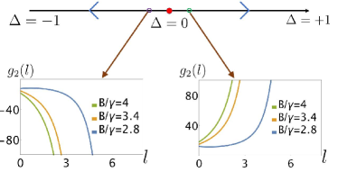
Figure 4: Schematic phase diagram for the measurement-only dynamics determined by the dimerization ΔΔ\Delta. The arrows indicate the RG flow to the two different fixed points Δ=±1Δplus-or-minus1\Delta=\pm 1 with a critical point (red dot) at Δ=0Δ0\Delta=0. The plots show The RG flow of g2subscript𝑔2g_{2} from (V) evaluated at different points (green and purple circles) indicating that the interaction is relevant in both cases, and it leads to area law of phases.

In the absence of unitary dynamics, J=0𝐽0J=0, the system is evolving entirely according to two competing sets of measurements: the set of odd and the set of even bond measurements. Notably, the J=0𝐽0J=0 limit of the model (20) coincides with the measurement-only case studied in Refs. 10, 18 where monitored and post-selected limits follow very different behaviours. In particular, finite-size scaling reveals that the monitored system belongs to a different universality class from the fully post-selected model [10].

Post-selected limit—

The fully post-selected dynamics are obtained by setting γ=0,B>0formulae-sequence𝛾0𝐵0\gamma=0,\,B>0 in Eq. (31). In this case, B𝐵B is just an overall time scale and the physics is entirely dictated by ΔΔ\Delta, given by (III). The effective Hamiltonian now reads:

=s=,a=1,2jsB(1+Δ(1)j)iχj(sa)χj+1(sa),subscript𝑠𝑎12subscript𝑗𝑠𝐵1Δsuperscript1𝑗𝑖subscriptsuperscript𝜒𝑠𝑎𝑗subscriptsuperscript𝜒𝑠𝑎𝑗1\displaystyle\mathcal{H}=-\sum_{\begin{subarray}{c}s=\uparrow,\,\downarrow\\ a=1,2\end{subarray}}\sum_{j}sB(1+\Delta(-1)^{j})i\chi^{(sa)}_{j}\chi^{(sa)}_{j+1}, (44)

Using the usual Jordan-Wigner transformation, the imaginary time evolution is, therefore, equivalent to 222 decoupled 1D1𝐷1D traverse field Ising models in either the bra (s=𝑠s=\downarrow) or ket (s=𝑠s=\uparrow) space.

The critical properties of the post-selected dynamics fall in the Ising universality class, and the critical exponent ν𝜈\nu that determines the divergence of the correlation length ξ|Δ|νsimilar-to𝜉superscriptΔ𝜈\xi\sim|\Delta|^{-\nu}, is ν=1𝜈1\nu=1. Away from criticality for Δ>0Δ0\Delta>0, the even parities are measured more strongly, and this phase is characterised by a pair of entangled Majorana fermions residing at the edges of a finite-length chain. This phase is associated with a log2subscript2\log_{2} topological entanglement entropy per replicated chain in the area-law phase.

On the other side Δ<0Δ0\Delta<0, the odd parities measurements are stronger and it features all Majorana being measured in pairs. This, therefore, corresponds to a topologically trivial phase with vanishing topological entanglement entropy.

Strong post-selection —

When γ0𝛾0\gamma\neq 0, the system does not follow any longer the deterministic dynamics from Eq. (44), but stochastic fluctuations inherent to the measurement process enter the system dynamics. With the partial post-selection introduced in Eq. (I), the parameter γ/B𝛾𝐵\gamma/B controls the amount of fluctuations (i.e. the fraction of quantum trajectories) allowed in the system’s dynamics. We can analyse the strong post-selected limit γ/B1much-less-than𝛾𝐵1\gamma/B\ll 1 with the bosonized Hamiltonian (V). As argued in Sec. V, the steady state of the system is governed by different equations for Δ=0Δ0\Delta=0 and Δ0Δ0\Delta\neq 0, so we address them separately.

For |Δ|>0Δ0|\Delta|>0, using the flow in (V), we observe that the cos\cos operator corresponding to the g2subscript𝑔2g_{2} coupling is in general relevant for Kρ+Kσ<4subscript𝐾𝜌subscript𝐾𝜎4K_{\rho}+K_{\sigma}<4, which we confirm by evaluating Eq. (V) numerically. The results are shown in Fig. 4 for different values of γ/B𝛾𝐵\gamma/B. The flow in the massive/gapped phase indicates an unbounded growth in the coupling g2subscript𝑔2g_{2}, which, moreover, does not change sign along the RG flow. When reinterpreting the RG flowing parameters in terms of the original parameters of the model B𝐵B, γ𝛾\gamma and ΔΔ\Delta via (V), this limit approaches the post-selected Hamiltonian (44) (γ0𝛾0\gamma\to 0). This indicates that the strong-PPS phase at finite γ𝛾\gamma with Δ>0Δ0\Delta>0 (Δ<0Δ0\Delta<0) is continuously connected to the gapped phase γ=0,Δ>0formulae-sequence𝛾0Δ0\gamma=0,\Delta>0 (γ=0,Δ<0formulae-sequence𝛾0Δ0\gamma=0,\Delta<0) of the post-selected model. The points |Δ|=1Δ1|\Delta|=1 are the two only stable fixed points in the measurement-only dynamics, as reported in the phase diagram in Fig. 4. We therefore expect that the universal properties of the strong-partial post-selected regime are inherited from Eq. (44), i.e. those of two uncorrelated copies of an Ising model.

This is the first main prediction of our theory: The MiPT remains in the same Ising-like university class for finite γ/B𝛾𝐵\gamma/B as long as the bosonized approximation for the theory remains valid. Physically, this predicts the stability of the post-selected MiPT universal feature against (weak) fluctuations induced by the stochasticity of the measurement.

For Δ=0Δ0\Delta=0, J=0𝐽0J=0, Eq. (V), together with the definition of Luttinger parameters in Eq. (V), implies that the g2=0subscript𝑔20g_{2}=0, and that the σ𝜎\sigma- and ρ𝜌\rho-modes decouple. The RG-flow is then standard [68], with the ρ𝜌\rho-mode flowing to a massive phase (gρsubscript𝑔𝜌g_{\rho}\to\infty), while the σ𝜎\sigma-mode, following an expansion around Kσ1+subscript𝐾𝜎superscript1K_{\sigma}\to 1^{+}, flows to gσ0subscript𝑔𝜎0g_{\sigma}\to 0, Kσ>1subscript𝐾𝜎1K_{\sigma}>1. Correlations in the overall theory are thus dominated by the σ𝜎\sigma-mode, which is a Gaussian-free theory displaying free Luttinger liquid criticality, with a logarithmic scaling of the entanglement entropy. Given that both σ𝜎\sigma- and ρ𝜌\rho-modes are massive for Δ0Δ0\Delta\neq 0, the ρ𝜌\rho-mode remains massive from Δ>0Δ0\Delta>0 to Δ<0Δ0\Delta<0 as long as γ0𝛾0\gamma\neq 0, while the σ𝜎\sigma-mode undergoes a transition. This is compatible with the behaviour of an Ising-like transition as discussed above.

From strong post-selection to monitored dynamics—

While our analytic theory predicts an Ising-like transition in the strong post-selected regime, numerical analysis indicates that the monitoring dynamics undergo a measurement-only transition of a different universality class with a critical exponent of ν=5/3𝜈53\nu=5/3 [10]. While our bosonized theory cannot access the full transition between post-selected (γ/B=0𝛾𝐵0\gamma/B=0) and monitored (γ/B𝛾𝐵\gamma/B\to\infty) dynamics due to the breakdown of bosonization at γsuperscript𝛾\gamma^{*}(cf. Sec. V), this divergence indicates a phase transition to a different phase [68].

This observation is corroborated numerically. We analyze the critical exponent ν:ξ|Δ|ν:𝜈similar-to𝜉superscriptΔ𝜈\nu:\xi\sim|\Delta|^{-\nu} of this measurement-only MiPT via finite-size scaling for generic γ/B𝛾𝐵\gamma/B. The details of the numerical methods are reported in Appendix G. The results are presented in Fig. 5 showing that ν1𝜈1\nu\approx 1 for strong PPS before deviating abruptly in a narrow range around γ/Bγ𝛾𝐵superscript𝛾\gamma/B\approx\gamma^{*} and approaching ν=5/3𝜈53\nu=5/3 when γ/B1much-greater-than𝛾𝐵1\gamma/B\gg 1. Surprisingly, numerical data shows that close to the transition, ν2.3>5/3𝜈2.353\nu\approx 2.3>5/3, before dropping back to ν=5/3𝜈53\nu=5/3 for larger γ/B𝛾𝐵\gamma/B.

Monitored limit, B=0𝐵0B=0

The monitored limit (B=0𝐵0B=0) is given by Eq. (IV), which, for the measurement only-case J=0𝐽0J=0, reduces to a XXZ𝑋𝑋𝑍XXZ-Hamiltonian with a dimerization in hopping term, also known as spin-Peierls model [68]. This model predicts a BKT transition at Δ=0Δ0\Delta=0 [68]. This differs from the Ising bosonized theory for the strong PPS. This difference is also consistent with the change in the symmetry of the model in the two limits, as discussed in Sec IV.

Note that the BKT transition (hence the scaling of the distorted partial purity or entanglement entropy) predicted by Eq. (IV) does not capture the correct universality class of the fully monitored dynamics. Indeed, in the limit B=0𝐵0B=0, it has been shown that the 222-replica model differs from the n1𝑛1n\to 1 limit for which the phase transition in the measurement-only limit is not known [18]. However, since for strong PPS the replicas completely decouple, the post-selected limit is independent of the replica number, and we expect that the stability of the post-selected phase and its breakdown should be captured in the 2-replica case considered here.
Refer to caption
Figure 5: The critical exponent ν𝜈\nu of the measurement only phase transition as a function of the degrees of PPS, γ/B𝛾𝐵\gamma/B. The pink region indicates where bosonization analysis is valid. The fully post-selected Ising critical exponent ν=1𝜈1\nu=1 is unchanged for a finite range of γ/B𝛾𝐵\gamma/B. The abrupt deviation form ν=1𝜈1\nu=1 occurs in the proximity of the breakdown of the bosonized theory at γ/Bγ=0.39𝛾𝐵superscript𝛾0.39\gamma/B\approx\gamma^{*}=0.39 (end of shaded region). The fully monitored critical exponent ν=5/3𝜈53\nu=5/3 is recovered only for γ/B𝛾𝐵\gamma/B\to\infty. The large error bars for γ/B1much-greater-than𝛾𝐵1\gamma/B\gg 1 are due to the large fluctuation due to the increasing trajectory-to-trajectory fluctuations in this regime.

VI.2 Partial post-selected monitoring with unitary dynamics

No-dimerization case, Δ=0Δ0\Delta=0

To analyze the effect of unitary dynamics on the system, we start by considering the case where dimerization is absent, Δ=0,J2>0,γ>0formulae-sequenceΔ0formulae-sequencesuperscript𝐽20𝛾0\Delta=0,J^{2}>0,\gamma>0. In this case, the RG flow in Eq. (V) keeps g2=0subscript𝑔20g_{2}=0, the ρ𝜌\rho-mode and σ𝜎\sigma-mode decouple as indicated by Hbossubscript𝐻𝑏𝑜𝑠H_{bos} and Eq. (V), and the Luttinger parameters Kρsubscript𝐾𝜌K_{\rho} and Kρsubscript𝐾𝜌K_{\rho} in (V) are both initially larger than unity. At the leading order, the RG flow signals that bossubscriptbos\mathcal{H}_{\text{bos}} is gapless for Kϵ>1subscript𝐾italic-ϵ1K_{\epsilon}>1. Evaluating (V) numerically reveals that one of the sectors is always massless. Given the decoupling between the two sectors, in general limt|ρˇ(2)(t)\lim\limits_{t\to\infty}\mathinner{|{\check{\rho}^{(2)}(t)}\rangle}\rangle will evolve to a tensor product of two ground states in the two sectors |ρ|σtensor-productketsubscript𝜌ketsubscript𝜎\mathinner{|{\mathcal{H}_{\rho}}\rangle}\otimes\mathinner{|{\mathcal{H}_{\sigma}}\rangle}. Thus, correlations w.r.t. bossubscriptbos\mathcal{H}_{\text{bos}} are dominated by the gapless power-law decaying sector, and the distorted partial purity μ¯¯k,𝐀=𝒞2,𝐀|et|ρ(2)(0)=𝕀|𝒞2,𝐀e(ρ+σ)t|𝕀subscript¯¯𝜇𝑘𝐀delimited-⟨⟩brasubscript𝒞2𝐀superscript𝑒𝑡ketsuperscript𝜌20delimited-⟨⟩bra𝕀subscript𝒞2𝐀superscript𝑒subscript𝜌subscript𝜎𝑡ket𝕀\overline{\overline{\mu}}_{k,\mathbf{A}}=\langle\mathinner{\langle{\mathcal{C}_{2,\mathbf{A}}}|}e^{-\mathcal{H}t}\mathinner{|{\rho^{(2)}(0)}\rangle}\rangle=\langle\mathinner{\langle{\mathbb{I}}|}\mathcal{C}_{2,\mathbf{A}}e^{-(\mathcal{H_{\rho}}+\mathcal{H_{\sigma}})t}\mathinner{|{\mathbb{I}}\rangle}\rangle will be dominated by correlation in the gapless sector. Therefore, we expect that the entanglement entropy will be dominated by the critical sector and will show a critical entanglement scaling.

This result differs from the predicted (logL)2superscriptlog𝐿2(\text{log}L)^{2} in Ref. 18 for the fully monitored case. The absence of (logL)2superscriptlog𝐿2(\text{log}L)^{2} scaling in strong PPS where bosonisation remains valid and could be traced back to the breaking of local parity j=aiχj(+a)χj(a),[j,]0formulae-sequencesubscript𝑗subscriptproduct𝑎𝑖subscriptsuperscript𝜒𝑎𝑗subscriptsuperscript𝜒𝑎𝑗commutatorsubscript𝑗0\mathcal{R}_{j}=\prod_{a}i\chi^{(+a)}_{j}\chi^{(-a)}_{j},\commutator{\mathcal{R}_{j}}{\mathcal{H}}\neq 0, which prohibits one to express \mathcal{H} solely as local SO(2N) generators. Consequently, \mathcal{H} is no longer described by the non-linear sigma model in [18] that gives the (logL)2superscriptlog𝐿2(\text{log}L)^{2} scaling.

Refer to caption
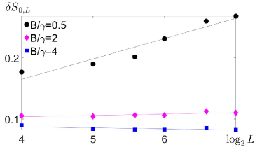
Figure 6: Scaling of the average entanglement entropy difference as a function of logL𝐿\log L for Δ=0Δ0\Delta=0 and J2/γ=0.25superscript𝐽2𝛾0.25J^{2}/\gamma=0.25. The dependence δS¯0,LlogLsimilar-to𝛿subscript¯𝑆0𝐿log𝐿\delta\overline{S}_{0,L}\sim\text{log}L or δS¯0,Lconst.similar-to𝛿subscript¯𝑆0𝐿const.\delta\overline{S}_{0,L}\sim\text{const.} distinguishes a (logL)2superscriptlog𝐿2(\text{log}L)^{2} from logL𝐿L scaling respectively. The lines of best fit of the data indicate a change of δS¯0,L𝛿subscript¯𝑆0𝐿\delta\overline{S}_{0,L} from linear increase (pink and black) to constant (blue) with increasing B/γ𝐵𝛾B/\gamma.

To confirm a change from logL𝐿\log L to (logL)2superscript𝐿2(\log L)^{2} with increasing J2superscript𝐽2J^{2}, we numerically analyze the scaling of the entropy along the no-dimerization line. The results are shown in Fig. 6. To distinguish the logL𝐿L-scaling from the (logL)2superscriptlog𝐿2(\text{log}L)^{2} one, we use as the indicator the difference in half-cut entanglement entropy δS0,LS0,L2/2S0,L/2𝛿subscript𝑆0𝐿subscript𝑆0subscript𝐿22subscript𝑆0𝐿2\delta S_{0,L}\equiv S_{0,L_{2}/2}-S_{0,L/2} (L2=2Lsubscript𝐿22𝐿L_{2}=2L[18], with δS¯0,LlogLsimilar-to𝛿subscript¯𝑆0𝐿log𝐿\delta\overline{S}_{0,L}\sim\text{log}L vs δS¯0,Lconst.similar-to𝛿subscript¯𝑆0𝐿const.\delta\overline{S}_{0,L}\sim\text{const.} dependence in the two cases respectively (see Appendix G). This analysis shows that, for fixed γ𝛾\gamma, increasing the degree of partial post-selection, B𝐵B, leads to a change from (log)2superscriptlog2(\text{log})^{2}-scaling to log\log-scaling. The change in the scaling behaviour happens approximately at the point where bosonization is expected to break down γ0.39superscript𝛾0.39\mathcal{\gamma}^{*}\approx 0.39. This is consistent with the picture in the previous section where the breakdown of bosonization at γ\gamma* signals a transition away from the university of the post selected model towards the universality of the monitored model which is captured by the non-linear sigma in Ref. 18.

General monitored-unitary dynamics, Δ0Δ0\Delta\neq 0

Refer to caption
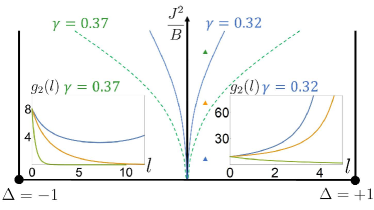
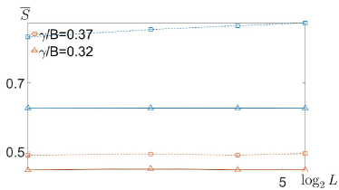
Figure 7: Schematic phase diagram obtained from the 2-replica approximation RG flow (V). A critical unitary strength Jcsubscript𝐽𝑐J_{c} separating the gapped area-law scaling phase (J2<Jc2superscript𝐽2subscriptsuperscript𝐽2𝑐J^{2}<J^{2}_{c}) from the critical logarithmic phase (J2>Jc2superscript𝐽2subscriptsuperscript𝐽2𝑐J^{2}>J^{2}_{c}) as reported for γ/B=0.32𝛾𝐵0.32\gamma/B=0.32 (green dotted line) and γ/B=0.37𝛾𝐵0.37\gamma/B=0.37 (blue line). The left and right insets show the flow of g2subscript𝑔2g_{2} under RG (V) for γ/B=0.37𝛾𝐵0.37\gamma/B=0.37 and γ/B=0.32𝛾𝐵0.32\gamma/B=0.32 respectively evaluated at J2/B=0.019superscript𝐽2𝐵0.019J^{2}/B=0.019 (blue),J2/B=0.20superscript𝐽2𝐵0.20J^{2}/B=0.20 (orange), and J2/B=0.38superscript𝐽2𝐵0.38J^{2}/B=0.38 (green), with Δ=0.07Δ0.07\Delta=0.07 in all cases. The irrelevance of g2subscript𝑔2g_{2} indicates a critical logarithmic scaling entanglement.

For generic strong PPS case with all |Δ|>0Δ0|\Delta|>0, J2>0superscript𝐽20J^{2}>0, and γ>0𝛾0\gamma>0, g2subscript𝑔2g_{2} is the main parameter which controls the entanglement scaling. From a numerical solution of the RG flow Eq. (V), we see that for small initial values, g2subscript𝑔2g_{2}, flows to either irrelevant at large J2/Bsuperscript𝐽2𝐵J^{2}/B or grows indefinitely for sufficiently small values of J2/Bsuperscript𝐽2𝐵J^{2}/B, (cf. Fig. 7). In the latter case, since the term governed by g2subscript𝑔2g_{2} is always more relevant than the gρsubscript𝑔𝜌g_{\rho} and gϕsubscript𝑔italic-ϕg_{\phi} ones, the physics is entirely governed by the g2subscript𝑔2g_{2} term, and the system is then in an area-law phase. When g2subscript𝑔2g_{2} flows to zero at large J2/Bsuperscript𝐽2𝐵J^{2}/B, the gϵsubscript𝑔italic-ϵg_{\epsilon} coupling term of cos(8ϕ)8italic-ϕ\cos(\sqrt{8}\phi) gaps at most one of the two sectors, leaving at least one sector gapless, and the phase remains critical as discussed in Sec. VI.1 for Δ=0Δ0\Delta=0.

The overall result for the phase diagram from the 2-replica approximation is schematically shown in Fig.7. For a fixed partial post-selection γ/B0𝛾𝐵0\gamma/B\neq 0, and non-zero dimerization Δ0Δ0\Delta\neq 0, we find critical values of J2superscript𝐽2J^{2} beyond which |g2|subscript𝑔2|g_{2}| grows indefinitely, corresponding to a critical-scaling phase. This phase expands when the retaining a larger subset of quantum trajectories (i.e. increasing γ/B𝛾𝐵\gamma/B). The results from the RG analysis of the 2-replica model are also confirmed by the numerical evaluation of the entanglement entropy scaling in appendix G, Fig. 12. This expansion is understood as a result of the system exploring a larger extent of the Hilbert space as more trajectories are retained. This imposes fewer constraints on the unitary dynamics in generating large-scale entanglement, and is consistent with similar numerical findings with deterministic unitary dynamics [10].

VII discussion and conlcusion

In this work, we have analysed the steady-state out-of-equilibrium phases of a monitored many-body quantum system when only part of the measurement readouts is retained (partial post-selection). We have first developed a general equation for the evolution of a quantum system under partial postselection of continuous Gaussian measurements, named Partial-Post-Selected Stochastic Schrödinger Equation (PPS-SSE) — cf. eq.(I), in which a parameter continuously bridges between the fully monitored and fully post-selected limits. Since the two limits are known to give rise to MiPT of different universality classes, we have studied such crossover for a specific model of free Gaussian real fermions with random unitary dynamics. We analyzed the MiPT in a 222-replica approximation which captures the simplest non-linearity in the system’s state. Within the approximation, we derive the MiPT in terms of the low energy long-wavelength properties of and associated bosonised Hamiltonian in a 222-replica-Choi-duplicated space in the limit of strong partial post-selection — cf. Eq.(V).

We predict that in the strong PPS limit, the model presents MiPTs from area laws (with distinct quantum order) to a critical phase. We show that for strong yet finite partial post-selection, the phase diagram displays the same universal features as the post-selected model. In particular, In the absence of unitary dynamics, the transition reduces to an Ising-like transition with a logarithmic critical scaling at the transition point. The entangling phase displays a log\log scaling instead of log2superscript2\log^{2} in Ref. 18, with the only quantitative changes given by the expansion of the phase with critical scaling upon increasing the range of measurement outcomes retained — cf. Fig. 7. Notably, our theory predictions are limited by the validity of the bosonization which breaks down at finite values of the partial post-selection indicating a possible phase transition at that point. Numerical results corroborate this finding by showing an abrupt change in the universal scaling of the measurement-only transition at a similar value of partial post-selection — cf. Fig. 5.

Our theory and its prediction shed new light on MiPT. First, the developed PPS-SSE is the first continuous stochastic equation that offers a novel analytical approach to study the relation between the critical phenomena observed in stochastic monitored dynamics and deterministic non-Hermitian evolution, as well as a means to analyze the transition between the two. It can be therefore employed to explore the role of multiple trajectories in a variety of MiPTs. The underlying microscopic derivation can also be the basis for obtaining similar PPS for other measurement-induced dynamics, like quantum jumps [52, 57, 54].

Our findings for the Gaussian model indicate that the physics of post-selected measurement dynamics is robust against weak fluctuations induced by measurements. Our results suggest that different trajectories contribute different universal properties to the overall ensemble. It is interesting to explore the generality of this finding and the mechanism underpinning the transition from post-selected to monitored dynamics identified in this work.

Finally, the feasibility of observing robust MiPTs by retaining a fraction of quantum trajectories provides a possible route to tackle the experimental post-selection problem, by performing tomography of the average state of a fraction of trajectories as opposed to tracking the trajectory-by-trajectory entanglement entropy.

Acknowledgements.
We are grateful to M. Buchhold, S. Diehl, R. Fazio, M. Fava, A. Mesaros, M. Schiro, and K. Turkeshi for helpful discussions. A.R. acknowledges from the Royal Society, grant no. IECR2212041. Note added. During the completion of this manuscript, we became aware of a related work by Y. Le Gal, X. Turkeshi, and M. Schirò appearing on arxiv, numerically analyzing the stability of non-Hermitian dynamics in the context of quantum jump equation [75].

Appendix A PPS, shifted Gaussian and their time continuum limit

Here, we demonstrate how the time continuum is taken giving δλ=bλ𝛿𝜆𝑏𝜆\delta\lambda=b\lambda. From (6), the shift in mean δλ𝛿𝜆\delta\lambda of Prcsubscript𝑃subscript𝑟𝑐P_{r_{c}} has the following rcsubscript𝑟𝑐r_{c} dependence

δλ=Δ2πe(rc+λO^i)22Δ21+Erf[rc+λO^i2Δ]𝛿𝜆Δ2𝜋superscript𝑒superscriptsubscript𝑟𝑐𝜆delimited-⟨⟩subscript^𝑂𝑖22superscriptΔ21Erfdelimited-[]subscriptrc𝜆delimited-⟨⟩subscript^Oi2Δ\displaystyle\delta\lambda=\Delta\sqrt{\frac{2}{\pi}}\frac{e^{-\frac{(-r_{c}+\lambda\langle\hat{O}_{i}\rangle)^{2}}{2\Delta^{2}}}}{1+{\rm Erf\left[\frac{-r_{c}+\lambda\langle\hat{O}_{i}\rangle}{\sqrt{2}\Delta}\right]}} (A.1)

Since λ𝜆\lambda scales as λdtsimilar-to𝜆𝑑𝑡\lambda\sim\sqrt{dt}, we ask what is the dt𝑑𝑡dt dependence we need to assign to rcsubscript𝑟𝑐r_{c} in order that δλdtsimilar-to𝛿𝜆𝑑𝑡\delta\lambda\sim\sqrt{dt} which matches the scaling of λ𝜆\lambda in the Kraus operator. In other words, we are solving

e(x+aO^jdt)21+Erf[x+aO^jdt]=badtsuperscript𝑒superscript𝑥𝑎delimited-⟨⟩subscript^𝑂𝑗𝑑𝑡21Erfdelimited-[]𝑥𝑎delimited-⟨⟩subscript^𝑂𝑗𝑑𝑡𝑏𝑎𝑑𝑡\displaystyle\frac{e^{-(-x+a\langle\hat{O}_{j}\rangle\sqrt{dt})^{2}}}{1+{\rm Erf}\left[-x+a\langle\hat{O}_{j}\rangle\sqrt{dt}\right]}=ba\sqrt{dt} (A.2)

where x=rc(dt)2Δ𝑥subscript𝑟𝑐𝑑𝑡2Δx=\frac{r_{c}(dt)}{\sqrt{2}\Delta}, a=γ2Δ𝑎𝛾2Δa=\frac{\sqrt{\gamma}}{\sqrt{2}\Delta}. This choice of parameterising δλ𝛿𝜆\delta\lambda ensures that rcsubscript𝑟𝑐r_{c} depends negligibly on O^jdelimited-⟨⟩subscript^𝑂𝑗\langle\hat{O}_{j}\rangle as dt0𝑑𝑡0dt\rightarrow 0 which is advantageous from an experimental point of view. The dependence of rcsubscript𝑟𝑐r_{c} on dt𝑑𝑡dt according to (A.2) is shown in figure(8a) and it can be seen that rcdt0𝑑𝑡0subscript𝑟𝑐r_{c}\xrightarrow[]{dt\rightarrow 0}-\infty.

Refer to caption
(a)
Refer to caption
(b)
Figure 8: (a): dependence of x𝑥x, from (A.2), on dt𝑑𝑡dt, with b=1𝑏1b=1 and O^j=0.1delimited-⟨⟩subscript^𝑂𝑗0.1\langle\hat{O}_{j}\rangle=0.1. It can be seen that rcxsimilar-tosubscript𝑟𝑐𝑥r_{c}\sim x approaches -\infty in the time continuum limit dt0𝑑𝑡0dt\rightarrow 0. (b): dependence of b𝑏b, from (A.2), on rcsubscript𝑟𝑐r_{c} for various dt𝑑𝑡dt. As dt𝑑𝑡dt decreases, the same b𝑏b corresponds to a rcsubscript𝑟𝑐r_{c} in the more negative direction.

Analogous to λdt00𝑑𝑡0𝜆0\lambda\xrightarrow[]{dt\rightarrow 0}0 and γ𝛾\gamma is the parameter that captures measurement backaction, what captures PPS in time continuum is b𝑏b from (A.2) and its dependence on rcsubscript𝑟𝑐r_{c} for fixed dt𝑑𝑡dt is shown in figure(8b), and it is lower bounded b(rc=)=0𝑏subscript𝑟𝑐0b(r_{c}=-\infty)=0. Solving for (A.2), we arrive at (7).

Under this scaling, we find that the correction to variance also scales like δdtsimilar-to𝛿𝑑𝑡\delta\sim\sqrt{dt}. However unlike the unmodified mean λ𝜆\lambda which scales like λ=γdt𝜆𝛾𝑑𝑡\lambda=\sqrt{\gamma dt}, under this parametrization Δ=𝒪(dt0)Δ𝒪𝑑superscript𝑡0\Delta={\cal O}(dt^{0}) and hence we can safely set δ0𝛿0\delta\rightarrow 0.

In addition to the two-sample Kolmogorov-Smirnov test on the probability distribution in the main text, we have also verified numerically the shifted Gaussian approximation by considering a 2-qubit toy model. The toy model is described by the Hamiltonian H=σ1+σ2+σ2+σ1𝐻subscriptsuperscript𝜎1subscriptsuperscript𝜎2subscriptsuperscript𝜎2subscriptsuperscript𝜎1H=\sigma^{+}_{1}\sigma^{-}_{2}+\sigma^{+}_{2}\sigma^{-}_{1}, and the 2 qubits are subject to measurement operators (𝕀+(1)jσjz)/2,j=1,2formulae-sequence𝕀superscript1𝑗superscriptsubscript𝜎𝑗𝑧2𝑗12(\mathbb{I}+(-1)^{j}\sigma_{j}^{z})/2,j=1,2. Firstly for fixed b𝑏b in (7), two separate distributions of the steady state entanglement entropy is computed via 2 different ways: 1. the update of the state by the measurement operators is given by (2) with the probability distribution Prc(xj)subscript𝑃subscript𝑟𝑐subscript𝑥𝑗P_{r_{c}}(x_{j}) given by the truncated Gaussian, 2. the update of the state is computed via (I). Then, the 2 distribution are compared using the Two-sample Kolmogorov-Smirnov test. This is repeated for different values of ΔtΔ𝑡\Delta t, the time increment used. The results are shown in figure (9).
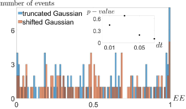
Refer to caption
Figure 9: Histogram of the steady state entanglement entropy distribution for various value of time increment in the numerics tt\d{t}. Blue colour are data evolved using truncated Gaussian distribution at rcsubscript𝑟𝑐r_{c}, red colour uses (I). The parameters used for this histogram are b=0.2,γ=0.5formulae-sequence𝑏0.2𝛾0.5b=0.2,\gamma=0.5 and dt=0.01𝑑𝑡0.01dt=0.01. The inset shows p𝑝p-values calculated for various dt𝑑𝑡dt using the Two-sample Kolmogorov-Smirnov test, revealing an upward trend for decreasing dt𝑑𝑡dt implying more overlapping between the data. For the values of b𝑏b and dt𝑑𝑡dt considered in the histogram, the null hypothesis cannot be rejected and the 2 different sets of data are statistically indistinguishable.

For completeness, we also display numerically the samplings from the truncated and shifted Gaussian in figure (10), together with the associated p-values calculated. It clearly display statistical equivalence for dt=0.001𝑑𝑡0.001dt=0.001.

Refer to caption
(a)
Refer to caption
(b)
Figure 10: Histograms of the truncated Gaussian Prc(xj)subscript𝑃subscript𝑟𝑐subscript𝑥𝑗P_{r_{c}}(x_{j}) and shifted Gaussian P¯(xj)¯𝑃subscript𝑥𝑗\underline{P}(x_{j}) in (6). (a): samplings drawn from the truncated Gaussian (blue) and the shifted Gaussian (red) for dt=0.05𝑑𝑡0.05dt=0.05 and the null hypothesis is rejected at a significance level of 0.05. The p-value from KS2 sample test is 0.000.000.00. (b): similar to (a) but samples generated with dt=0.001𝑑𝑡0.001dt=0.001. The p-value is 0.310.310.31 and the null hypothesis cannot be rejected, indicating the distribution is statistically indistinguishable. The values of the parameters used here are Oj=1,b=1formulae-sequencedelimited-⟨⟩subscript𝑂𝑗1𝑏1\langle O_{j}\rangle=1,b=1 and γ=0.5𝛾0.5\gamma=0.5 and we used 500050005000 samplings of the distributions.

Appendix B Continuous measurement as non-Herm noises and PPS on Gaussian average

The procedures we are using here is an extension to [18], and we make explicit link to the discrete time description of continuous measurement in (2), and extending it to PPS. To begin with, we start from (2) and changes some of the factor slightly for later convenience:

k^j(x,λ)subscript^𝑘𝑗𝑥𝜆\displaystyle\hat{k}_{j}(x,\lambda) =𝒩jexp((x2λO^j)24Δ2)absentsubscript𝒩𝑗superscript𝑥2𝜆subscript^𝑂𝑗24superscriptΔ2\displaystyle=\mathcal{N}_{j}\exp\left(-\frac{(x-2\lambda\hat{O}_{j})^{2}}{4\Delta^{2}}\right)
k^j(x,λ)|ψtsubscript^𝑘𝑗𝑥𝜆ketsubscript𝜓𝑡\displaystyle\hat{k}_{j}(x,\lambda)\mathinner{|{\psi_{t}}\rangle} =𝒩~jexp(x24Δ2)exp(λO^jxΔ2)|ψtabsentsubscript~𝒩𝑗superscript𝑥24superscriptΔ2𝜆subscript^𝑂𝑗𝑥superscriptΔ2ketsubscript𝜓𝑡\displaystyle=\tilde{\mathcal{N}}_{j}\exp\left(-\frac{x^{2}}{4\Delta^{2}}\right)\exp\left(\frac{\lambda\hat{O}_{j}x}{\Delta^{2}}\right)\mathinner{|{\psi_{t}}\rangle} (B.1)

An initial normalised density matrix ρ0subscript𝜌0\rho_{0} is updated as

k^j(x,λ)ρ0k^j(x,λ)Tr[k^j(x,λ)ρ0k^j(x,λ)]=ρˇx,λTr[ρˇx,λ]subscript^𝑘𝑗𝑥𝜆subscript𝜌0subscriptsuperscript^𝑘𝑗𝑥𝜆tracesubscript^𝑘𝑗𝑥𝜆subscript𝜌0subscriptsuperscript^𝑘𝑗𝑥𝜆subscriptˇ𝜌𝑥𝜆tracesubscriptˇ𝜌𝑥𝜆\displaystyle\frac{\hat{k}_{j}(x,\lambda)\rho_{0}\hat{k}^{\dagger}_{j}(x,\lambda)}{\Tr[\hat{k}_{j}(x,\lambda)\rho_{0}\hat{k}^{\dagger}_{j}(x,\lambda)]}=\frac{\check{\rho}_{x,\lambda}}{\Tr[\check{\rho}_{x,\lambda}]} (B.2)

The average density matrix ρ¯¯𝜌\overline{\rho} across all measurement outcome at a particular time step is

ρ¯¯𝜌\displaystyle\overline{\rho} =𝑑xρˇx,λTr[ρˇx,λ]P(x,λ)absentsuperscriptsubscriptdifferential-d𝑥subscriptˇ𝜌𝑥𝜆tracesubscriptˇ𝜌𝑥𝜆𝑃𝑥𝜆\displaystyle=\int_{-\infty}^{\infty}dx\frac{\check{\rho}_{x,\lambda}}{\Tr[\check{\rho}_{x,\lambda}]}P(x,\lambda)
ρ¯¯𝜌\displaystyle\overline{\rho} =𝑑xk^j(x,λ)ρ0k^j(x,λ)absentsuperscriptsubscriptdifferential-d𝑥subscript^𝑘𝑗𝑥𝜆subscript𝜌0subscriptsuperscript^𝑘𝑗𝑥𝜆\displaystyle=\int_{-\infty}^{\infty}dx\hat{k}_{j}(x,\lambda)\rho_{0}\hat{k}^{\dagger}_{j}(x,\lambda)
=𝒩~j2𝑑xexp(x22Δ2)exp(xλO^jΔ2)ρ0exp(xλO^jΔ2)absentsuperscriptsubscript~𝒩𝑗2superscriptsubscriptdifferential-d𝑥superscript𝑥22superscriptΔ2𝑥𝜆subscript^𝑂𝑗superscriptΔ2subscript𝜌0𝑥𝜆subscript^𝑂𝑗superscriptΔ2\displaystyle=\tilde{\mathcal{N}}_{j}^{2}\int_{-\infty}^{\infty}dx\exp\left(-\frac{x^{2}}{2\Delta^{2}}\right)\exp\left(\frac{x\lambda\hat{O}_{j}}{\Delta^{2}}\right)\rho_{0}\exp\left(\frac{x\lambda\hat{O}_{j}}{\Delta^{2}}\right) (B.3)

which implies

𝑑xk^j(x,λ)k^j(x,λ)superscriptsubscriptdifferential-d𝑥subscriptsuperscript^𝑘𝑗𝑥𝜆subscript^𝑘𝑗𝑥𝜆\displaystyle\int_{-\infty}^{\infty}dx\hat{k}^{\dagger}_{j}(x,\lambda)\hat{k}_{j}(x,\lambda) =𝕀absent𝕀\displaystyle=\mathbb{I}
𝒩~j2𝑑xexp(x22Δ2)exp(x2λO^jΔ2)superscriptsubscript~𝒩𝑗2superscriptsubscriptdifferential-d𝑥superscript𝑥22superscriptΔ2𝑥2𝜆subscript^𝑂𝑗superscriptΔ2\displaystyle\tilde{\mathcal{N}}_{j}^{2}\int_{-\infty}^{\infty}dx\exp\left(-\frac{x^{2}}{2\Delta^{2}}\right)\exp\left(\frac{x2\lambda\hat{O}_{j}}{\Delta^{2}}\right) =𝕀absent𝕀\displaystyle=\mathbb{I} (B.4)

Rewriting

Δ2=Δ2λ/δt,x=MjΔ2andγ=λ/Δ2=λ2/Δ2δtformulae-sequencesuperscriptΔ2superscriptΔ2𝜆𝛿𝑡𝑥subscript𝑀𝑗superscriptΔ2and𝛾𝜆superscriptΔ2superscript𝜆2superscriptΔ2𝛿𝑡\displaystyle\Delta^{2}=\Delta^{\prime 2}\lambda/\delta t,x=M_{j}\Delta^{\prime 2}\text{and}\ \gamma=\lambda/\Delta^{\prime 2}=\lambda^{2}/\Delta^{2}\delta t (B.5)

(B) becomes

𝒩~j2𝑑Mjexp(Mj2δt2γ)exp(2MjO^jδt)superscriptsubscript~𝒩𝑗2superscriptsubscriptdifferential-dsubscript𝑀𝑗superscriptsubscript𝑀𝑗2𝛿𝑡2𝛾2subscript𝑀𝑗subscript^𝑂𝑗𝛿𝑡\displaystyle\tilde{\mathcal{N}}_{j}^{2}\int_{-\infty}^{\infty}dM_{j}\exp\left(-\frac{M_{j}^{2}\delta t}{2\gamma}\right)\exp\left(2M_{j}\hat{O}_{j}\delta t\right) =𝕀absent𝕀\displaystyle=\mathbb{I} (B.6)

and one can interpret that the Kraus operator is alternatively described by

k^¯(Mj)=exp(MjO^jδt)¯^𝑘subscript𝑀𝑗subscript𝑀𝑗subscript^𝑂𝑗𝛿𝑡\displaystyle\overline{\hat{k}}(M_{j})=\exp\left(M_{j}\hat{O}_{j}\delta t\right)
𝑑μ(Mj)k^¯(Mj)k^¯(Mj)=𝕀superscriptsubscriptdifferential-d𝜇subscript𝑀𝑗superscript¯^𝑘subscript𝑀𝑗¯^𝑘subscript𝑀𝑗𝕀\displaystyle\int_{-\infty}^{\infty}d\mu(M_{j})\overline{\hat{k}}^{\dagger}(M_{j})\overline{\hat{k}}(M_{j})=\mathbb{I} (B.7)

and normalised over the Gaussian measure dμ(Mj)dMjexp(Mj2δt2γ)proportional-to𝑑𝜇subscript𝑀𝑗𝑑subscript𝑀𝑗superscriptsubscript𝑀𝑗2𝛿𝑡2𝛾d\mu(M_{j})\propto dM_{j}\exp\left(-\frac{M_{j}^{2}\delta t}{2\gamma}\right), which describes a Gaussian random variable Mjsubscript𝑀𝑗M_{j} with mean 𝔼G[Mj]=0subscript𝔼𝐺delimited-[]subscript𝑀𝑗0\mathbb{E}_{G}[M_{j}]=0 and variance 𝔼G[Mj2]=γ/δtsubscript𝔼𝐺delimited-[]superscriptsubscript𝑀𝑗2𝛾𝛿𝑡\mathbb{E}_{G}[M_{j}^{2}]=\gamma/\delta t.

The readout of a continuous measurement is now represented by the variable Mjsubscript𝑀𝑗M_{j}, and its backaction on the system is given by the Kraus operator in (B). To generalise it to a time process, we first give Mj(tl)subscript𝑀𝑗subscript𝑡𝑙M_{j}(t_{l}) a time index tl=lδtsubscript𝑡𝑙𝑙𝛿𝑡t_{l}=l\delta t. Then, an initial density matrix ρ0subscript𝜌0\rho_{0} evolves from time t0=0subscript𝑡00t_{0}=0 to tN=T=Nδtsubscript𝑡𝑁𝑇𝑁𝛿𝑡t_{N}=T=N\delta t as

ρˇM(T)=l=1l=Nk^¯(Mj(tl))ρ(0)k^¯(Mj(tl)),subscriptˇ𝜌𝑀𝑇superscriptsubscriptproduct𝑙1𝑙𝑁¯^𝑘subscript𝑀𝑗subscript𝑡𝑙𝜌0superscript¯^𝑘subscript𝑀𝑗subscript𝑡𝑙\displaystyle\check{\rho}_{M}(T)=\prod_{l=1}^{l=N}\overline{\hat{k}}(M_{j}(t_{l}))\rho(0)\overline{\hat{k}}^{\dagger}(M_{j}(t_{l})), (B.8)

where M𝑀M labels the quantum trajectory. In the time continuum limit, (B.8) becomes

ρˇM=K(t)ρ(0)K(t)subscriptˇ𝜌𝑀𝐾𝑡𝜌0superscript𝐾𝑡\displaystyle\check{\rho}_{M}=K(t)\rho(0)K^{\dagger}(t)
K(t)=exp[i0T𝑑tH(t)]=exp[i0T𝑑tiMj(t)O^j]𝐾𝑡𝑖superscriptsubscript0𝑇differential-dsuperscript𝑡𝐻superscript𝑡𝑖superscriptsubscript0𝑇differential-dsuperscript𝑡𝑖subscript𝑀𝑗superscript𝑡subscript^𝑂𝑗\displaystyle K(t)=\exp[-i\int_{0}^{T}dt^{\prime}H(t^{\prime})]=\exp[-i\int_{0}^{T}dt^{\prime}iM_{j}(t^{\prime})\hat{O}_{j}] (B.9)

and 𝔼G[Mj(t)]=0,𝔼G[Mj(t)Mj(t)]=γδ(tt)formulae-sequencesubscript𝔼𝐺delimited-[]subscript𝑀𝑗𝑡0subscript𝔼𝐺delimited-[]subscript𝑀𝑗𝑡subscript𝑀𝑗superscript𝑡𝛾𝛿𝑡superscript𝑡\mathbb{E}_{G}[M_{j}(t)]=0,\,\mathbb{E}_{G}[M_{j}(t)M_{j}(t^{\prime})]=\gamma\delta(t-t^{\prime}). From (B), we observe that the overall effect of a continuous measurement generates a random non-Hermitian Hamiltonian H(t)=iMj(t)O^j𝐻𝑡𝑖subscript𝑀𝑗𝑡subscript^𝑂𝑗H(t)=iM_{j}(t)\hat{O}_{j} in time. Generalisation to multiple measurement j=1L𝑗1𝐿j=1\dots L, and including another competing set, follows the same line as each process is independent to each other, and we arrive at (20) in the main text.

In the case of PPS, we saw, in Appendix A, that PPS shifts the mean of the random variable x𝑥x by bλ𝑏𝜆b\lambda. We can interpret this as a shift in the mean of the measure. Using the relationship (B.5)

dμ(Mj)𝑑𝜇subscript𝑀𝑗\displaystyle d\mu(M_{j}) PPSdxexp((xbλ)22Δ2)𝑃𝑃𝑆absent𝑑𝑥superscript𝑥𝑏𝜆22superscriptΔ2\displaystyle\xrightarrow[]{PPS}dx\exp\left(-\frac{(x-b\lambda)^{2}}{2\Delta^{2}}\right)
dMjexp((Mjbγ)2δt2γ)proportional-toabsent𝑑subscript𝑀𝑗superscriptsubscript𝑀𝑗𝑏𝛾2𝛿𝑡2𝛾\displaystyle\propto dM_{j}\exp\left(-\frac{(M_{j}-b\gamma)^{2}\delta t}{2\gamma}\right) (B.10)

we arrive at the final line where the mean of the Gaussian average is shifted 𝔼G[Mj]=bγ=Bsubscript𝔼𝐺delimited-[]subscript𝑀𝑗𝑏𝛾𝐵\mathbb{E}_{G}[M_{j}]=b\gamma=B, as required from PPS. The generalisation to multiple weak continuous measurement is straightforward, with different measurement corresponds to different non-Hermitian noises and taking the time continuum limit gives (III) (since noises from different measurements are independent from each other, cross product between different noise vanishes in time continuum limit).

Appendix C operator-state correspondence and replica majorana Hamiltonian

In this appendix and below, we distinguish the ket or bra space in the Choi–Jamiołkowski isomorphism by σ=±𝜎plus-or-minus\sigma=\pm to replace \uparrow and \downarrow in the main text.

The Choi–Jamiołkowski isomorphism maps an operator to a duplicated Hilbert space:

O^=i,jOi,j|ij|Choii,jOi,j|i|j=|O^^𝑂subscript𝑖𝑗subscript𝑂𝑖𝑗ket𝑖bra𝑗𝐶𝑜𝑖subscript𝑖𝑗tensor-productsubscript𝑂𝑖𝑗ket𝑖ket𝑗ket^𝑂\displaystyle\hat{O}=\sum_{i,j}O_{i,j}\mathinner{|{i}\rangle}\mathinner{\langle{j}|}\xrightarrow[]{Choi}\sum_{i,j}O_{i,j}\mathinner{|{i}\rangle}\otimes\mathinner{|{j}\rangle}=\mathinner{|{\hat{O}}\rangle} (C.1)

Under Choi–Jamiołkowski isomorphism, the trace operation between 2 operators becomes a transition amplitude:

Tr[A^B^]ChoiA^|B^𝐶𝑜𝑖Trdelimited-[]superscript^𝐴^𝐵inner-product^𝐴^𝐵\displaystyle\text{Tr}[\hat{A}^{\dagger}\hat{B}]\xrightarrow[]{Choi}\langle\hat{A}|\hat{B}\rangle (C.2)

hence equ (27). When dealing with density matrix ρ𝜌\rho, the action of some operator on the density matrix becomes action on the Choi state:

A^ρ^𝐴𝜌\displaystyle\hat{A}\rho =i,j,kAi,jρj,k|ik|Choii,j,kAi,jρj,k|i|k=A^𝕀|ρabsentsubscript𝑖𝑗𝑘subscript𝐴𝑖𝑗subscript𝜌𝑗𝑘ket𝑖bra𝑘𝐶𝑜𝑖subscript𝑖𝑗𝑘subscript𝐴𝑖𝑗subscript𝜌𝑗𝑘ket𝑖ket𝑘tensor-product^𝐴𝕀ket𝜌\displaystyle=\sum_{i,j,k}A_{i,j}\rho_{j,k}\mathinner{|{i}\rangle}\mathinner{\langle{k}|}\xrightarrow[]{Choi}\sum_{i,j,k}A_{i,j}\rho_{j,k}\mathinner{|{i}\rangle}\mathinner{|{k}\rangle}=\hat{A}\otimes\mathbb{I}\mathinner{|{\rho}\rangle}
ρA^𝜌^𝐴\displaystyle\rho\hat{A} Choi𝕀A^T|ρ,B^ρA^ChoiB^A^T|ρformulae-sequence𝐶𝑜𝑖absenttensor-product𝕀superscript^𝐴𝑇ket𝜌𝐶𝑜𝑖^𝐵𝜌^𝐴tensor-product^𝐵superscript^𝐴𝑇ket𝜌\displaystyle\xrightarrow[]{Choi}\mathbb{I}\otimes\hat{A}^{T}\mathinner{|{\rho}\rangle},\ \hat{B}\rho\hat{A}\xrightarrow[]{Choi}\hat{B}\otimes\hat{A}^{T}\mathinner{|{\rho}\rangle} (C.3)

and hence (25). Writing out explicitly the average dynamics of n𝑛n-replica described by (III):

𝔼G(PPS)[(K(t)K(t))n]|ρn(0)\displaystyle\mathbb{E}^{(PPS)}_{G}[\left(K(t)\otimes K^{*}(t)\right)^{\otimes n}]\mathinner{|{\rho^{n}(0)}\rangle}\rangle
=\displaystyle= 𝔼G(PPS)[exp(i0tHn(t)𝑑t)]subscriptsuperscript𝔼𝑃𝑃𝑆𝐺delimited-[]𝑖superscriptsubscript0𝑡subscript𝐻𝑛superscript𝑡differential-dsuperscript𝑡\displaystyle\mathbb{E}^{(PPS)}_{G}\left[\exp\left(-i\int_{0}^{t}H_{n}(t^{\prime})dt^{\prime}\right)\right]
Hn(t)subscript𝐻𝑛superscript𝑡\displaystyle H_{n}(t^{\prime}) =σ=±a=1nj[Jj(t)+iσMj(t)]iχj(σa)χj+1(σa)absentsubscript𝜎plus-or-minus𝑎1𝑛subscript𝑗delimited-[]subscript𝐽𝑗superscript𝑡𝑖𝜎subscript𝑀𝑗superscript𝑡𝑖superscriptsubscript𝜒𝑗𝜎𝑎superscriptsubscript𝜒𝑗1𝜎𝑎\displaystyle=\sum_{\begin{subarray}{c}\sigma=\pm\\ a=1\dots n\end{subarray}}\sum_{j}\left[J_{j}(t^{\prime})+i\sigma M_{j}(t^{\prime})\right]i\chi_{j}^{(\sigma a)}\chi_{j+1}^{(\sigma a)} (C.4)

where σ𝜎\sigma distinguish ket/bra space, a𝑎a for replica: χj(a)=𝕀2a+1χj𝕀2a,χj(+a)=𝕀2aχj𝕀2a+1formulae-sequencesuperscriptsubscript𝜒𝑗𝑎tensor-productsuperscript𝕀tensor-productabsent2𝑎1superscriptsubscript𝜒𝑗superscript𝕀tensor-productabsent2𝑎superscriptsubscript𝜒𝑗𝑎tensor-productsuperscript𝕀tensor-productabsent2𝑎subscript𝜒𝑗superscript𝕀tensor-productabsent2𝑎1\chi_{j}^{(-a)}=\mathbb{I}^{\otimes 2a+1}\otimes\chi_{j}^{*}\otimes\mathbb{I}^{\otimes 2a},\chi_{j}^{(+a)}=\mathbb{I}^{\otimes 2a}\otimes\chi_{j}\otimes\mathbb{I}^{\otimes 2a+1}. Up to this point, the Majorana operator χj(σa)superscriptsubscript𝜒𝑗𝜎𝑎\chi_{j}^{(\sigma a)} is not well defined as they anti-commute within the same branch and replica, while commuting each other in different branch or replica. To resolve this, one should first map the Majorana to spin Hilbert space, then define new Majorana operators which differs from the one in (C) by a Klein factor which plays the role of Pauli string in the replica space [18]. Calling the proper Majorana operators in the replica space as χj(σa),{χj(σa),χl(σa)}=δj,lδσ,σδa,asuperscriptsubscript𝜒𝑗𝜎𝑎superscriptsubscript𝜒𝑗𝜎𝑎superscriptsubscript𝜒𝑙superscript𝜎superscript𝑎subscript𝛿𝑗𝑙subscript𝛿𝜎superscript𝜎subscript𝛿𝑎superscript𝑎\chi_{j}^{\prime(\sigma a)},\ \{\chi_{j}^{\prime(\sigma a)},\chi_{l}^{\prime(\sigma^{\prime}a^{\prime})}\}=\delta_{j,l}\delta_{\sigma,\sigma^{\prime}}\delta_{a,a^{\prime}}, the bilinear product χj(σa)χj+1(σa)=χj(σa)χj+1(σa)superscriptsubscript𝜒𝑗𝜎𝑎superscriptsubscript𝜒𝑗1𝜎𝑎superscriptsubscript𝜒𝑗𝜎𝑎superscriptsubscript𝜒𝑗1𝜎𝑎\chi_{j}^{(\sigma a)}\chi_{j+1}^{(\sigma a)}=\chi_{j}^{\prime(\sigma a)}\chi_{j+1}^{\prime(\sigma a)} is preserved with no extra factor.

To evaluate (C), we expand it using cumulant expansion up to 2nd order eAexp[A+1/2(A2A2)]delimited-⟨⟩superscript𝑒𝐴delimited-⟨⟩𝐴12delimited-⟨⟩superscript𝐴2superscriptdelimited-⟨⟩𝐴2\langle e^{A}\rangle\approx\exp[\langle A\rangle+1/2(\langle A^{2}\rangle-\langle A\rangle^{2})] and note that the Guassian measure now centred at bγj𝑏subscript𝛾𝑗b\gamma_{j}. With a slight abuse of notation by calling the new anti-commuting Majorana as χj(σa)χj(σa)superscriptsubscript𝜒𝑗𝜎𝑎superscriptsubscript𝜒𝑗𝜎𝑎\chi_{j}^{\prime(\sigma a)}\rightarrow\chi_{j}^{(\sigma a)}, for n=2𝑛2n=2 we arrive at (31).

Finally, the boundary state |𝒞2,𝐀,|𝕀\mathinner{|{\mathcal{C}_{2,\mathbf{A}}}\rangle}\rangle,\mathinner{|{\mathbb{I}}\rangle}\rangle have the following properties with the Pauli matrices in the replica space σα,j(a),α=x,y,za=1,2formulae-sequencesuperscriptsubscript𝜎𝛼𝑗𝑎𝛼𝑥𝑦𝑧𝑎12\sigma_{\alpha,j}^{(a)}\ ,\alpha=x,y,z\ a=1,2 [18]:

σα,j(a)𝕀σα,j(a)=𝕀superscriptsubscript𝜎𝛼𝑗𝑎𝕀superscriptsubscript𝜎𝛼𝑗𝑎𝕀\displaystyle\sigma_{\alpha,j}^{(a)}\mathbb{I}\sigma_{\alpha,j}^{(a)}=\mathbb{I} Choiiχj(+a)χj(a)|𝕀=|𝕀\displaystyle\xrightarrow[]{Choi}i\chi_{j}^{(+a)}\chi_{j}^{(-a)}\mathinner{|{\mathbb{I}}\rangle}\rangle=\mathinner{|{\mathbb{I}}\rangle}\rangle
σα,j(a)𝒞2,𝐀σα,j(a)=𝒞2,𝐀superscriptsubscript𝜎𝛼𝑗𝑎subscript𝒞2𝐀superscriptsubscript𝜎𝛼𝑗𝑎subscript𝒞2𝐀\displaystyle\sigma_{\alpha,j}^{(a)}\mathcal{C}_{2,\mathbf{A}}\sigma_{\alpha,j}^{(a)}=\mathcal{C}_{2,\mathbf{A}} Choiiχj(+a)χj(a)|𝒞2,𝐀=|𝒞2,𝐀,j𝐀\displaystyle\xrightarrow[]{Choi}i\chi_{j}^{(+a)}\chi_{j}^{(-a)}\mathinner{|{\mathcal{C}_{2,\mathbf{A}}}\rangle}\rangle=\mathinner{|{\mathcal{C}_{2,\mathbf{A}}}\rangle}\rangle,\ j\notin\mathbf{A}
σα,j(2)𝒞2,𝐀σα,j(1)=𝒞2,𝐀superscriptsubscript𝜎𝛼𝑗2subscript𝒞2𝐀superscriptsubscript𝜎𝛼𝑗1subscript𝒞2𝐀\displaystyle\sigma_{\alpha,j}^{(2)}\mathcal{C}_{2,\mathbf{A}}\sigma_{\alpha,j}^{(1)}=\mathcal{C}_{2,\mathbf{A}} Choiiχj(+2)χj(1)|𝒞2,𝐀=|𝒞2,𝐀,j𝐀\displaystyle\xrightarrow[]{Choi}-i\chi_{j}^{(+2)}\chi_{j}^{(-1)}\mathinner{|{\mathcal{C}_{2,\mathbf{A}}}\rangle}\rangle=\mathinner{|{\mathcal{C}_{2,\mathbf{A}}}\rangle}\rangle,\ j\in\mathbf{A}
σα,j(1)𝒞2,𝐀σα,j(2)=𝒞2,𝐀superscriptsubscript𝜎𝛼𝑗1subscript𝒞2𝐀superscriptsubscript𝜎𝛼𝑗2subscript𝒞2𝐀\displaystyle\sigma_{\alpha,j}^{(1)}\mathcal{C}_{2,\mathbf{A}}\sigma_{\alpha,j}^{(2)}=\mathcal{C}_{2,\mathbf{A}} Choiiχj(+1)χj(2)|𝒞2,𝐀=|𝒞2,𝐀,j𝐀\displaystyle\xrightarrow[]{Choi}i\chi_{j}^{(+1)}\chi_{j}^{(-2)}\mathinner{|{\mathcal{C}_{2,\mathbf{A}}}\rangle}\rangle=\mathinner{|{\mathcal{C}_{2,\mathbf{A}}}\rangle}\rangle,\ j\in\mathbf{A} (C.5)

Appendix D Solution for 2-replica for monitored case

Recall that the effective Hamiltonian without PPS reads

\displaystyle\mathcal{H} =12jJ2(σ=±a=1,2iχj(σa)χj+1(σa))2γj(σ=±a=1,2σiχj(σa)χj+1(σa))2absent12subscript𝑗superscript𝐽2superscriptsubscript𝜎plus-or-minus𝑎12𝑖subscriptsuperscript𝜒𝜎𝑎𝑗subscriptsuperscript𝜒𝜎𝑎𝑗12subscript𝛾𝑗superscriptsubscript𝜎plus-or-minus𝑎12𝜎𝑖subscriptsuperscript𝜒𝜎𝑎𝑗subscriptsuperscript𝜒𝜎𝑎𝑗12\displaystyle=\frac{1}{2}\sum_{j}J^{2}(\sum_{\begin{subarray}{c}\sigma=\pm\\ a=1,2\end{subarray}}i\chi^{(\sigma a)}_{j}\chi^{(\sigma a)}_{j+1})^{2}-\gamma_{j}(\sum_{\begin{subarray}{c}\sigma=\pm\\ a=1,2\end{subarray}}\sigma i\chi^{(\sigma a)}_{j}\chi^{(\sigma a)}_{j+1})^{2} (D.1)

one can write it entirely as local SO(4) generators defined using Majorana operators:

Sjα,β=i2[χjα,χjβ]subscriptsuperscript𝑆𝛼𝛽𝑗𝑖2commutatorsuperscriptsubscript𝜒𝑗𝛼superscriptsubscript𝜒𝑗𝛽\displaystyle S^{\alpha,\beta}_{j}=\frac{i}{2}\commutator{\chi_{j}^{\alpha}}{\chi_{j}^{\beta}} (D.2)

and for generic J2,γsuperscript𝐽2𝛾J^{2},\gamma, only a subset of (D.2) commutes with \mathcal{H} [18, 65]. An important set of local symmetry which will become clear are the local on-site parity j=aiγ(+a)γ(a),[j,]=0formulae-sequencesubscript𝑗subscriptproduct𝑎𝑖superscript𝛾𝑎superscript𝛾𝑎commutatorsubscript𝑗0\mathcal{R}_{j}=\prod_{a}i\gamma^{(+a)}\gamma^{(-a)},\commutator{\mathcal{R}_{j}}{\mathcal{H}}=0.

One can readily define the following spin-1/2 operators:

Σμ=12𝐜¯jσμ𝐜¯jsuperscriptΣ𝜇12superscriptsubscript¯𝐜𝑗subscript𝜎𝜇subscript¯𝐜𝑗\displaystyle\Sigma^{\mu}=\frac{1}{2}\underline{\mathbf{c}}_{j}^{\dagger}\sigma_{\mu}\underline{\mathbf{c}}_{j} (D.3)

where σα,α=x,y,zformulae-sequencesubscript𝜎𝛼𝛼𝑥𝑦𝑧\sigma_{\alpha}\ ,\alpha=x,y,z are the usual Pauli matrices and 𝐜¯j=(cj,,cj,)Tsubscript¯𝐜𝑗superscriptsubscript𝑐𝑗subscript𝑐𝑗𝑇\underline{\mathbf{c}}_{j}=(c_{j,\uparrow},c_{j,\downarrow})^{T}. The other spin-1/2 generators is associated with the η𝜂\eta spin in the Hubbard model, generated via Shiba transformation [72, 76].

ηjz=12(cj,cj,+cj,cj,1),ηj+=cj,cj,formulae-sequencesuperscriptsubscript𝜂𝑗𝑧12subscriptsuperscript𝑐𝑗subscript𝑐𝑗subscriptsuperscript𝑐𝑗subscript𝑐𝑗1superscriptsubscript𝜂𝑗subscriptsuperscript𝑐𝑗subscriptsuperscript𝑐𝑗\displaystyle\eta_{j}^{z}=\frac{1}{2}\left(c^{\dagger}_{j,\uparrow}c_{j,\uparrow}+c^{\dagger}_{j,\downarrow}c_{j,\downarrow}-1\right)\ ,\ \eta_{j}^{+}=c^{\dagger}_{j,\uparrow}c^{\dagger}_{j,\downarrow} (D.4)

these two species of SU(2) generators stems from the fact that SO(4)[\cong[SU(2)×\timesSU(2)]/2]/\mathbb{Z}_{2}. The quotient by 2subscript2\mathbb{Z}_{2} comes from the criterion that

j[ηjz+Σjz]=jcj,cj,L2subscript𝑗delimited-[]superscriptsubscript𝜂𝑗𝑧superscriptsubscriptΣ𝑗𝑧subscript𝑗subscriptsuperscript𝑐𝑗subscript𝑐𝑗𝐿2\displaystyle\sum_{j}\left[\eta_{j}^{z}+\Sigma_{j}^{z}\right]=\sum_{j}c^{\dagger}_{j,\uparrow}c_{j,\uparrow}-\frac{L}{2}\ \in\mathbb{Z} (D.5)

and ηjz,Σjzsuperscriptsubscript𝜂𝑗𝑧superscriptsubscriptΣ𝑗𝑧\eta_{j}^{z},\Sigma_{j}^{z} can either be both integer or both half-integer (assuming L𝐿L is even). Recalling that the local parity operator j=±1subscript𝑗plus-or-minus1\mathcal{R}_{j}=\pm 1 commutes with \mathcal{H}, constructing the projector Πj,+=12(1+j)subscriptΠ𝑗121subscript𝑗\Pi_{j,+}=\frac{1}{2}\left(1+\mathcal{R}_{j}\right) we observe that

Πj,+ΣjμΠj,+=0, whileΠj,+ηjμΠj,+=ηjμsubscriptΠ𝑗superscriptsubscriptΣ𝑗𝜇subscriptΠ𝑗0, whilesubscriptΠ𝑗superscriptsubscript𝜂𝑗𝜇subscriptΠ𝑗superscriptsubscript𝜂𝑗𝜇\displaystyle\Pi_{j,+}\Sigma_{j}^{\mu}\Pi_{j,+}=0\ \text{, while}\ \Pi_{j,+}\eta_{j}^{\mu}\Pi_{j,+}=\eta_{j}^{\mu} (D.6)

hence the two different SU(2) Σμ,ημsuperscriptΣ𝜇superscript𝜂𝜇\Sigma^{\mu},\eta^{\mu} acts on j=1subscript𝑗minus-or-plus1\mathcal{R}_{j}=\mp 1 sector respectively. The choice of the initial state |ρ(0)=|𝕀,j|𝕀=+1|𝕀\mathinner{|{\rho(0)}\rangle}\rangle=\mathinner{|{\mathbb{I}}\rangle}\rangle,\mathcal{R}_{j}\mathinner{|{\mathbb{I}}\rangle}\rangle=+1\mathinner{|{\mathbb{I}}\rangle}\rangle fixes the sector and should match the sector the boundary state is in. To complete the prove that ημsuperscript𝜂𝜇\eta^{\mu} (and hence ΣμsuperscriptΣ𝜇\Sigma^{\mu}) are spin-1/2 operators, we demonstrate that the total spin operator has eigenvalue:

ηjx2+ηjy2+ηjx2|𝕀=43|𝕀=S(1+S)|𝕀\displaystyle{\eta_{j}^{x}}^{2}+{\eta_{j}^{y}}^{2}+{\eta_{j}^{x}}^{2}\mathinner{|{\mathbb{I}}\rangle}\rangle=\frac{4}{3}\mathinner{|{\mathbb{I}}\rangle}\rangle=S(1+S)\mathinner{|{\mathbb{I}}\rangle}\rangle (D.7)

where S=1/2𝑆12S=1/2.

The SO(4) generators in (D.2) can be expressed in term of these two SU(2) generators i.e. S+1,+2=2(Σz+ηz)superscript𝑆122superscriptΣ𝑧superscript𝜂𝑧S^{+1,+2}=2(\Sigma^{z}+\eta^{z}). Writing (D.1) in terms of (D.4) and (D.3), we arrive at (IV) and the physics can readily be extracted via usual means i.e. Bethe Ansatz and bosonisation.

Appendix E effective spin Hamiltonian and bosonisation details

As mentioned in the main text, there are two conserved charges [jγj(σ1)γj(σ2),]commutatorsubscript𝑗superscriptsubscript𝛾𝑗𝜎1superscriptsubscript𝛾𝑗𝜎2\commutator{\sum_{j}\gamma_{j}^{(\sigma 1)}\gamma_{j}^{(\sigma 2)}}{\mathcal{H}}, which suggest the following 2 complex fermions:

cj,=γj(+1)+iγj(+2)2,cj,=γj(1)iγj(2)2formulae-sequencesubscriptsuperscript𝑐𝑗superscriptsubscript𝛾𝑗1𝑖superscriptsubscript𝛾𝑗22subscriptsuperscript𝑐𝑗superscriptsubscript𝛾𝑗1𝑖superscriptsubscript𝛾𝑗22\displaystyle c^{\dagger}_{j,\uparrow}=\frac{\gamma_{j}^{(+1)}+i\gamma_{j}^{(+2)}}{2}\ ,\ c^{\dagger}_{j,\downarrow}=\frac{\gamma_{j}^{(-1)}-i\gamma_{j}^{(-2)}}{2} (E.1)

Written in terms of the complex fermions, it becomes [,Nσ]=0,Nσ=jcj,σcj,σ,σ=,formulae-sequencecommutatorsubscript𝑁𝜎0formulae-sequencesubscript𝑁𝜎subscript𝑗subscriptsuperscript𝑐𝑗𝜎subscript𝑐𝑗𝜎𝜎\commutator{\mathcal{H}}{N_{\sigma}}=0,\ N_{\sigma}=\sum_{j}c^{\dagger}_{j,\sigma}c_{j,\sigma},\ \sigma=\uparrow,\downarrow. These two conserved U(1)𝑈1U(1) charges will be the basis for abelian bosonisation later. Inserting this relationship and followed by an unitary transformation cj,(i)jcj,,cj,(i)jcj,formulae-sequencesubscriptsuperscript𝑐𝑗superscript𝑖𝑗subscriptsuperscript𝑐𝑗subscriptsuperscript𝑐𝑗superscript𝑖𝑗subscriptsuperscript𝑐𝑗c^{\dagger}_{j,\uparrow}\rightarrow(i)^{j}c^{\dagger}_{j,\uparrow},\ c^{\dagger}_{j,\downarrow}\rightarrow(-i)^{j}c^{\dagger}_{j,\downarrow}, the Majorana operators are transformed as:

i(γj(+1)γj+1(+1)+γj(+2)γj+1(+2))2(cj,cj+1,+cj+1,cj,)𝑖subscriptsuperscript𝛾1𝑗subscriptsuperscript𝛾1𝑗1subscriptsuperscript𝛾2𝑗subscriptsuperscript𝛾2𝑗12subscriptsuperscript𝑐𝑗subscript𝑐𝑗1subscriptsuperscript𝑐𝑗1subscript𝑐𝑗\displaystyle-i(\gamma^{(+1)}_{j}\gamma^{(+1)}_{j+1}+\gamma^{(+2)}_{j}\gamma^{(+2)}_{j+1})\rightarrow-2(c^{\dagger}_{j,\uparrow}c_{j+1,\uparrow}+c^{\dagger}_{j+1,\uparrow}c_{j,\uparrow})
i(γj(1)γj+1(1)+γj(2)γj+1(2))2(cj,cj+1,+cj+1,cj,)𝑖subscriptsuperscript𝛾1𝑗subscriptsuperscript𝛾1𝑗1subscriptsuperscript𝛾2𝑗subscriptsuperscript𝛾2𝑗12subscriptsuperscript𝑐𝑗subscript𝑐𝑗1subscriptsuperscript𝑐𝑗1subscript𝑐𝑗\displaystyle i(\gamma^{(-1)}_{j}\gamma^{(-1)}_{j+1}+\gamma^{(-2)}_{j}\gamma^{(-2)}_{j+1})\rightarrow-2(c^{\dagger}_{j,\downarrow}c_{j+1,\downarrow}+c^{\dagger}_{j+1,\downarrow}c_{j,\downarrow}) (E.2)

Inserting these into (31), we arrive at (33).

We now proceed to bosonise (33) w.r.t. the basis σ=,𝜎\sigma=\uparrow,\downarrow. We first compute terms corresponding to no dimerisation 𝒪(Δ)0𝒪superscriptΔ0\mathcal{O}(\Delta)^{0}. H0subscript𝐻0H_{0} the kinetic part gives the usual free Luttinger liquid Hamiltonian with K=1𝐾1K=1:

H0=vF2πσ=,x(xθσ)2+(xϕσ)2subscript𝐻0subscript𝑣𝐹2𝜋subscript𝜎subscript𝑥superscriptsubscript𝑥subscript𝜃𝜎2superscriptsubscript𝑥subscriptitalic-ϕ𝜎2\displaystyle H_{0}=\frac{v_{F}}{2\pi}\sum_{\sigma=\uparrow,\downarrow}\int_{x}(\partial_{x}\theta_{\sigma})^{2}+(\partial_{x}\phi_{\sigma})^{2} (E.3)

With bosonisation, we can investigate the strong PPS limit where J2,γBmuch-less-thansuperscript𝐽2𝛾𝐵J^{2},\gamma\ll B . This is the limit at which the excitation is small compare to the Fermi energy and bosonisation remains valid. As bosonising a lattice model will inevitably generate term whose appearance depends directly on the filling fraction, the filling fraction is determined by utilising the properties in (C) which gives

𝕀|iχj(+1)χj(2)|𝕀=0delimited-⟨⟩bra𝕀𝑖superscriptsubscript𝜒𝑗1superscriptsubscript𝜒𝑗2ket𝕀0\displaystyle\langle\mathinner{\langle{\mathbb{I}}|}i\chi_{j}^{(+1)}\chi_{j}^{(-2)}\mathinner{|{\mathbb{I}}\rangle}\rangle=0
𝕀|χj(+1)χj(+2)|𝕀=0delimited-⟨⟩bra𝕀superscriptsubscript𝜒𝑗1superscriptsubscript𝜒𝑗2ket𝕀0\displaystyle\langle\mathinner{\langle{\mathbb{I}}|}-\chi_{j}^{(+1)}\chi_{j}^{(+2)}\mathinner{|{\mathbb{I}}\rangle}\rangle=0
𝕀|(cj,+cj,)(cj,cj,)|𝕀=0delimited-⟨⟩bra𝕀subscriptsuperscript𝑐𝑗subscript𝑐𝑗subscriptsuperscript𝑐𝑗subscript𝑐𝑗ket𝕀0\displaystyle\langle\mathinner{\langle{\mathbb{I}}|}(c^{\dagger}_{j,\uparrow}+c_{j,\uparrow})(c^{\dagger}_{j,\uparrow}-c_{j,\uparrow})\mathinner{|{\mathbb{I}}\rangle}\rangle=0
𝕀|12cj,cj,)|𝕀=0\displaystyle\langle\mathinner{\langle{\mathbb{I}}|}1-2c^{\dagger}_{j,\uparrow}c_{j,\uparrow})\mathinner{|{\mathbb{I}}\rangle}\rangle=0 (E.4)

similarly for cj,subscriptsuperscript𝑐𝑗c^{\dagger}_{j,\downarrow} and the boundary state |𝒞2,𝐀\mathinner{|{\mathcal{C}_{2,\mathbf{A}}}\rangle}\rangle. Therefore, this specifies that we are dealing with half filling kF=π/2subscript𝑘𝐹𝜋2k_{F}=\pi/2 and some term that oscillates with e4ikFxsuperscript𝑒4𝑖subscript𝑘𝐹𝑥e^{4ik_{F}x} should in fact be kept.

The term Humksubscript𝐻𝑢𝑚𝑘H_{umk} in (33) becomes

Humkproportional-tosubscript𝐻𝑢𝑚𝑘absent\displaystyle H_{umk}\propto σ=,j(cj,σcj+1,σ+cj+1,σcj,σ)2subscript𝜎𝑗superscriptsubscriptsuperscript𝑐𝑗𝜎subscript𝑐𝑗1𝜎subscriptsuperscript𝑐𝑗1𝜎subscript𝑐𝑗𝜎2\displaystyle\sum_{\begin{subarray}{c}\sigma=\uparrow,\downarrow\\ j\end{subarray}}(c^{\dagger}_{j,\sigma}c_{j+1,\sigma}+c^{\dagger}_{j+1,\sigma}c_{j,\sigma})^{2}
=\displaystyle= 2σ=,j(cj,σcj,σ12)(cj+1,σcj+1,σ12)2subscript𝜎𝑗subscriptsuperscript𝑐𝑗𝜎subscript𝑐𝑗𝜎12subscriptsuperscript𝑐𝑗1𝜎subscript𝑐𝑗1𝜎12\displaystyle-2\sum_{\begin{subarray}{c}\sigma=\uparrow,\downarrow\\ j\end{subarray}}(c^{\dagger}_{j,\sigma}c_{j,\sigma}-\frac{1}{2})(c^{\dagger}_{j+1,\sigma}c_{j+1,\sigma}-\frac{1}{2})
\displaystyle\approx 2aσ=,x2π2(xϕσ)22(2πα)2cos4ϕσ2𝑎subscript𝜎subscript𝑥2superscript𝜋2superscriptsubscript𝑥subscriptitalic-ϕ𝜎22superscript2𝜋𝛼2𝑐𝑜𝑠4subscriptitalic-ϕ𝜎\displaystyle-2a\sum_{\sigma=\uparrow,\downarrow}\int_{x}\frac{2}{\pi^{2}}(\partial_{x}\phi_{\sigma})^{2}-\frac{2}{(2\pi\alpha)^{2}}cos4\phi_{\sigma} (E.5)

while Hmsubscript𝐻𝑚H_{m} gives

Hmsubscript𝐻𝑚\displaystyle H_{m} j(cj,cj+1,+h.c.)(cj,cj+1,+h.c.)\displaystyle\propto\sum_{j}(c^{\dagger}_{j,\uparrow}c_{j+1,\uparrow}+h.c.)(c^{\dagger}_{j,\downarrow}c_{j+1,\downarrow}+h.c.)
\displaystyle\approx ax[42πϕ+e2ikFx2πα2iei2ϕ(x)e2ikFx2πα2iei2ϕ(x)]𝑎subscript𝑥delimited-[]42𝜋subscriptitalic-ϕsuperscript𝑒2𝑖subscript𝑘𝐹𝑥2𝜋𝛼2𝑖superscript𝑒𝑖2subscriptitalic-ϕ𝑥superscript𝑒2𝑖subscript𝑘𝐹𝑥2𝜋𝛼2𝑖superscript𝑒𝑖2subscriptitalic-ϕ𝑥\displaystyle a\int_{x}\Bigg{[}\frac{4}{2\pi}\nabla\phi_{\uparrow}+\frac{e^{2ik_{F}x}}{2\pi\alpha}2ie^{-i2\phi_{\uparrow}(x)}-\frac{e^{-2ik_{F}x}}{2\pi\alpha}2ie^{i2\phi_{\uparrow}(x)}\Bigg{]}
×[]\displaystyle\times\Bigg{[}\uparrow\rightarrow\downarrow\Bigg{]}
=\displaystyle= ax4π2ϕϕ+8(2πα)2cos[2(ϕϕ)]𝑎subscript𝑥4superscript𝜋2subscriptitalic-ϕsubscriptitalic-ϕ8superscript2𝜋𝛼2𝑐𝑜𝑠delimited-[]2subscriptitalic-ϕsubscriptitalic-ϕ\displaystyle a\int_{x}\frac{4}{\pi^{2}}\nabla\phi_{\uparrow}\nabla\phi_{\downarrow}+\frac{8}{(2\pi\alpha)^{2}}cos[2(\phi_{\uparrow}-\phi_{\downarrow})]
8(2πα)2cos[2(ϕ+ϕ)]8superscript2𝜋𝛼2𝑐𝑜𝑠delimited-[]2subscriptitalic-ϕsubscriptitalic-ϕ\displaystyle-\frac{8}{(2\pi\alpha)^{2}}cos[2(\phi_{\uparrow}+\phi_{\downarrow})] (E.6)

The cos4ϕσ𝑐𝑜𝑠4subscriptitalic-ϕ𝜎cos4\phi_{\sigma} is highly irrelevant under RG compare to the cosines from (E) and therefore can be discarded without much concerns.

We now move on to terms coming from dimerisation 𝒪(Δ)1𝒪superscriptΔ1\mathcal{O}(\Delta)^{1}. This amounts to looking for e2ikFxsuperscript𝑒2𝑖subscript𝑘𝐹𝑥e^{2ik_{F}x} components from bosonisation as (1)j=e2ikFxsuperscript1𝑗superscript𝑒2𝑖subscript𝑘𝐹𝑥(-1)^{j}=e^{2ik_{F}x}. Bosonising H0subscript𝐻0H_{0} gives the following term

2BΔjη=,(1)j(cj+1,ηcj,η+h.c.)\displaystyle-2B\Delta\sum_{\begin{subarray}{c}j\\ \eta=\uparrow,\downarrow\end{subarray}}(-1)^{j}(c^{\dagger}_{j+1,\eta}c_{j,\eta}+h.c.)
16aBΔπ(2πα)2η=,xsin2ϕηabsent16𝑎𝐵Δ𝜋superscript2𝜋𝛼2subscript𝜂subscript𝑥𝑠𝑖𝑛2subscriptitalic-ϕ𝜂\displaystyle\approx\frac{16aB\Delta\pi}{(2\pi\alpha)^{2}}\sum_{\eta=\uparrow,\downarrow}\int_{x}sin2\phi_{\eta} (E.7)

which is highly relevant. Humksubscript𝐻𝑢𝑚𝑘H_{umk} requires some attention and bosonisation should be treated carefully within fermion normal ordering ψ(x)Rψ(x)R¯=[2π(xx)]1,ψ(x)Lψ(x)L¯=[2π(xx)]1formulae-sequence¯𝜓subscript𝑥𝑅superscript𝜓subscriptsuperscript𝑥𝑅superscriptdelimited-[]2𝜋𝑥superscript𝑥1¯𝜓subscript𝑥𝐿superscript𝜓subscriptsuperscript𝑥𝐿superscriptdelimited-[]2𝜋𝑥superscript𝑥1\underline{\psi(x)_{R}\psi^{\dagger}(x^{\prime})_{R}}=\left[2\pi(x-x^{\prime})\right]^{-1},\ \underline{\psi(x)_{L}\psi^{\dagger}(x^{\prime})_{L}}=-\left[2\pi(x-x^{\prime})\right]^{-1} [77]. In the end, this give Humksubscript𝐻𝑢𝑚𝑘H_{umk} the following term

4ΓΔjη=,(1)j(cj,ηcj,η12)(cj+1,ηcj+1,η12)4ΓΔsubscript𝑗𝜂superscript1𝑗subscriptsuperscript𝑐𝑗𝜂subscript𝑐𝑗𝜂12subscriptsuperscript𝑐𝑗1𝜂subscript𝑐𝑗1𝜂12\displaystyle-4\Gamma\Delta\sum_{\begin{subarray}{c}j\\ \eta=\uparrow,\downarrow\end{subarray}}(-1)^{j}(c^{\dagger}_{j,\eta}c_{j,\eta}-\frac{1}{2})(c^{\dagger}_{j+1,\eta}c_{j+1,\eta}-\frac{1}{2})
=\displaystyle= 16aΓΔ(2πα)2η=,xsin2ϕη(x)16𝑎ΓΔsuperscript2𝜋𝛼2subscript𝜂subscript𝑥𝑠𝑖𝑛2subscriptitalic-ϕ𝜂𝑥\displaystyle\frac{-16a\Gamma\Delta}{(2\pi\alpha)^{2}}\sum_{\eta=\uparrow,\downarrow}\int_{x}sin2\phi_{\eta}(x) (E.8)

and a less relevant operator (xϕ)2sin2ϕsuperscriptsubscript𝑥italic-ϕ2𝑠𝑖𝑛2italic-ϕ(\partial_{x}\phi)^{2}sin2\phi have been discarded. For Hmsubscript𝐻𝑚H_{m}, the 2kF2subscript𝑘𝐹2k_{F} component gives terms ϕcos2ϕ+ϕcos2ϕsubscriptitalic-ϕ𝑐𝑜𝑠2subscriptitalic-ϕsubscriptitalic-ϕ𝑐𝑜𝑠2subscriptitalic-ϕ~{}\nabla\phi_{\uparrow}cos2\phi_{\downarrow}+\nabla\phi_{\downarrow}cos2\phi_{\uparrow} which is irrelevant in the current model: By power counting, it can be seen that its dimension is 1+Kρ+Kσ21subscript𝐾𝜌subscript𝐾𝜎21+\frac{K_{\rho}+K_{\sigma}}{2}. Since Kρ,Kσ1subscript𝐾𝜌subscript𝐾𝜎1K_{\rho},K_{\sigma}\geq 1 from (V), this term is simply irrelevant in the current setting.

Inserting these results, and performing a unitary rotation to the charge and spin degree of freedom ϕρ=ϕ+ϕ2,ϕσ=ϕϕ2formulae-sequencesubscriptitalic-ϕ𝜌subscriptitalic-ϕsubscriptitalic-ϕ2subscriptitalic-ϕ𝜎subscriptitalic-ϕsubscriptitalic-ϕ2\phi_{\rho}=\frac{\phi_{\uparrow}+\phi_{\downarrow}}{\sqrt{2}},\ \phi_{\sigma}=\frac{\phi_{\uparrow}-\phi_{\downarrow}}{\sqrt{2}}, we arrive at (V).

Appendix F RG flow for Sine-Gordon Hamiltonian

The procedure here is a real space renormalisation group procedure that follows closely with Ref. 68, 74. We will also demonstrate explicitly that the unmklapp term Humksubscript𝐻umkH_{\mathrm{umk}} in (33) is way less relevant. The form of Sine-Gordon Hamiltonian we encounter from Umklapp term and dimerisation has the following form

H=𝐻absent\displaystyle H= i=1,212π𝑑xuiKi(xθi)2+uiKi(xϕi)2subscript𝑖1212𝜋differential-d𝑥subscript𝑢𝑖subscript𝐾𝑖superscriptsubscript𝑥subscript𝜃𝑖2subscript𝑢𝑖subscript𝐾𝑖superscriptsubscript𝑥subscriptitalic-ϕ𝑖2\displaystyle\sum_{i=1,2}\frac{1}{2\pi}\int dx\ u_{i}K_{i}(\partial_{x}\theta_{i})^{2}+\frac{u_{i}}{K_{i}}(\partial_{x}\phi_{i})^{2}
+2g(2πα)2𝑑xcos(βϕ1)cos(βϕ2)2𝑔superscript2𝜋𝛼2differential-d𝑥𝑐𝑜𝑠𝛽subscriptitalic-ϕ1𝑐𝑜𝑠𝛽subscriptitalic-ϕ2\displaystyle+\frac{2g}{(2\pi\alpha)^{2}}\int dx\ cos(\beta\phi_{1})cos(\beta\phi_{2}) (F.1)

where Ki,uisubscript𝐾𝑖subscript𝑢𝑖K_{i},u_{i} are the Luttinger parameter and velocity of two different bosonic field species ϕi,θisubscriptitalic-ϕ𝑖subscript𝜃𝑖\phi_{i},\theta_{i}. β𝛽\beta is the frequency and it is 88\sqrt{8} for the umklapp term while 22\sqrt{2} for dimerisaiton term. To begin with, consider the following correlation function

R(r1r2)=eia22ϕ1(r1)eia22ϕ1(r2)H𝑅subscript𝑟1subscript𝑟2subscriptdelimited-⟨⟩superscript𝑒𝑖superscript𝑎22subscriptitalic-ϕ1subscript𝑟1superscript𝑒𝑖superscript𝑎22subscriptitalic-ϕ1subscript𝑟2𝐻\displaystyle R(r_{1}-r_{2})=\langle e^{ia^{2}\sqrt{2}\phi_{1}(r_{1})}e^{-ia^{2}\sqrt{2}\phi_{1}(r_{2})}\rangle_{H} (F.2)

The average with respect to the free kinetic part of the Hamiltonian H0=i=1,212π𝑑xuiKi(xθi)2+uiKi(xϕi)2subscript𝐻0subscript𝑖1212𝜋differential-d𝑥subscript𝑢𝑖subscript𝐾𝑖superscriptsubscript𝑥subscript𝜃𝑖2subscript𝑢𝑖subscript𝐾𝑖superscriptsubscript𝑥subscriptitalic-ϕ𝑖2H_{0}=\sum_{i=1,2}\frac{1}{2\pi}\int dx\ u_{i}K_{i}(\partial_{x}\theta_{i})^{2}+\frac{u_{i}}{K_{i}}(\partial_{x}\phi_{i})^{2} is

eia22ϕi(r1)eia22ϕi(r2)H0=ea2KiF1,i(r1r2)(αr1r2)a2Kisubscriptdelimited-⟨⟩superscript𝑒𝑖superscript𝑎22subscriptitalic-ϕ𝑖subscript𝑟1superscript𝑒𝑖superscript𝑎22subscriptitalic-ϕ𝑖subscript𝑟2subscript𝐻0superscript𝑒superscript𝑎2subscript𝐾𝑖subscript𝐹1𝑖subscript𝑟1subscript𝑟2similar-to-or-equalssuperscript𝛼subscript𝑟1subscript𝑟2superscript𝑎2subscript𝐾𝑖\displaystyle\langle e^{ia^{2}\sqrt{2}\phi_{i}(r_{1})}e^{-ia^{2}\sqrt{2}\phi_{i}(r_{2})}\rangle_{H_{0}}=e^{-a^{2}K_{i}F_{1,i}(r_{1}-r_{2})}\simeq(\frac{\alpha}{r_{1}-r_{2}})^{a^{2}K_{i}}
[ϕ(r1)ϕ(r2)]2H0=KiF1,i(r1r2),F1,i(r)=12log[x2+(ui|τ|+α)2α2]formulae-sequencesubscriptdelimited-⟨⟩superscriptdelimited-[]italic-ϕsubscript𝑟1italic-ϕsubscript𝑟22subscript𝐻0subscript𝐾𝑖subscript𝐹1𝑖subscript𝑟1subscript𝑟2subscript𝐹1𝑖𝑟12logdelimited-[]superscript𝑥2superscriptsubscript𝑢𝑖𝜏𝛼2superscript𝛼2\displaystyle\langle[\phi(r_{1})-\phi(r_{2})]^{2}\rangle_{H_{0}}=K_{i}F_{1,i}(r_{1}-r_{2})\ ,\ F_{1,i}(r)=\frac{1}{2}\text{log}\left[\frac{x^{2}+(u_{i}|\tau|+\alpha)^{2}}{\alpha^{2}}\right] (F.3)

Since the Hamiltonian is separable in the kinetic part, averages w.r.t. to the free kinetic Hamiltonian can be performed separably f(ϕ1)g(ϕ2)H0=f(ϕ1)H0,1g(ϕ2)H0,2subscriptdelimited-⟨⟩𝑓subscriptitalic-ϕ1𝑔subscriptitalic-ϕ2subscript𝐻0subscriptdelimited-⟨⟩𝑓subscriptitalic-ϕ1subscript𝐻01subscriptdelimited-⟨⟩𝑔subscriptitalic-ϕ2subscript𝐻02\langle f(\phi_{1})g(\phi_{2})\rangle_{H_{0}}=\langle f(\phi_{1})\rangle_{H_{0,1}}\langle g(\phi_{2})\rangle_{H_{0,2}}. The full action reads:

S=i=1,212πKi𝑑x𝑑τ1ui(τϕ)2+ui(xϕ)2S0,1+S0,2+2g(2πα)2𝑑x𝑑τcos(βϕ1)cos(βϕ2)𝑆superscriptsubscript𝑖1212𝜋subscript𝐾𝑖differential-d𝑥differential-d𝜏1subscript𝑢𝑖superscriptsubscript𝜏italic-ϕ2subscript𝑢𝑖superscriptsubscript𝑥italic-ϕ2subscript𝑆01subscript𝑆022𝑔superscript2𝜋𝛼2differential-d𝑥differential-d𝜏𝑐𝑜𝑠𝛽subscriptitalic-ϕ1𝑐𝑜𝑠𝛽subscriptitalic-ϕ2\displaystyle S=\overbrace{\sum_{i=1,2}\frac{1}{2\pi K_{i}}\int dxd\tau\frac{1}{u_{i}}(\partial_{\tau}\phi)^{2}+u_{i}(\partial_{x}\phi)^{2}}^{S_{0,1}+S_{0,2}}+\frac{2g}{(2\pi\alpha)^{2}}\int dxd\tau\ cos(\beta\phi_{1})cos(\beta\phi_{2}) (F.4)

θ𝜃\theta has been integrated out as it merely contributes a constant which cancels out in the expectation value. As u1u2subscript𝑢1subscript𝑢2u_{1}\neq u_{2}, there is an extra non-trivial factor towards the end. If we expand in powers of g𝑔g the first order is 0 and stopping at second order, the partition function is

Z𝑍\displaystyle Z =𝒟ϕ1𝒟ϕ2eSabsent𝒟subscriptitalic-ϕ1𝒟subscriptitalic-ϕ2superscript𝑒𝑆\displaystyle=\int\mathcal{D}\phi_{1}\mathcal{D}\phi_{2}e^{-S}
=𝒟ϕ1𝒟ϕ2eS0,1S0,2[10\displaystyle=\int\mathcal{D}\phi_{1}\mathcal{D}\phi_{2}e^{-S_{0,1}-S_{0,2}}\Bigg{[}1-0
+132(2g(2πα)2)2d2rd2r′′i=1,2ϵ1,ϵ2=±eiϵ1βϕi(r)eiϵ2βϕi(r)]\displaystyle+\frac{1}{32}\left(\frac{2g}{(2\pi\alpha)^{2}}\right)^{2}\int d^{2}r^{\prime}d^{2}r^{\prime\prime}\prod_{i=1,2}\sum_{\epsilon_{1},\epsilon_{2}=\pm}e^{i\epsilon_{1}\beta\phi_{i}(r^{\prime})}e^{-i\epsilon_{2}\beta\phi_{i}(r^{\prime})}\Bigg{]} (F.5)

d2r=dxdτsuperscript𝑑2𝑟𝑑𝑥𝑑𝜏d^{2}r=dxd\tau is different to the conventional definition for now. Expanding F.2 in g𝑔g and stopping at 2nd order, we have

eia22ϕ1(r1)eia22ϕ1(r2)Hea2K1F1,1(r1r2)subscriptdelimited-⟨⟩superscript𝑒𝑖superscript𝑎22subscriptitalic-ϕ1subscript𝑟1superscript𝑒𝑖superscript𝑎22subscriptitalic-ϕ1subscript𝑟2𝐻superscript𝑒superscript𝑎2subscript𝐾1subscript𝐹11subscript𝑟1subscript𝑟2\displaystyle\langle e^{ia^{2}\sqrt{2}\phi_{1}(r_{1})}e^{-ia^{2}\sqrt{2}\phi_{1}(r_{2})}\rangle_{H}\approx e^{-a^{2}K_{1}F_{1,1}(r_{1}-r_{2})}
+18(g(2πα)2)2[d2rd2r′′eia22ϕ1(r1)eia22ϕ1(r2)i=1,2ϵ1,ϵ2=±eiϵ1βϕi(r)eiϵ2βϕi(r)H0\displaystyle+\frac{1}{8}\left(\frac{g}{(2\pi\alpha)^{2}}\right)^{2}\Bigg{[}\int d^{2}r^{\prime}d^{2}r^{\prime\prime}\langle e^{ia^{2}\sqrt{2}\phi_{1}(r_{1})}e^{-ia^{2}\sqrt{2}\phi_{1}(r_{2})}\prod_{i=1,2}\sum_{\epsilon_{1},\epsilon_{2}=\pm}e^{i\epsilon_{1}\beta\phi_{i}(r^{\prime})}e^{-i\epsilon_{2}\beta\phi_{i}(r^{\prime})}\rangle_{H_{0}}
ea2K1F1,1(r1r2)i=1,2ϵ1,ϵ2=±eiϵ1βϕi(r)eiϵ2βϕi(r)H0]\displaystyle-e^{-a^{2}K_{1}F_{1,1}(r_{1}-r_{2})}\langle\prod_{i=1,2}\sum_{\epsilon_{1},\epsilon_{2}=\pm}e^{i\epsilon_{1}\beta\phi_{i}(r^{\prime})}e^{-i\epsilon_{2}\beta\phi_{i}(r^{\prime})}\rangle_{H_{0}}\Bigg{]}
=ea2K1F1,1(r1r2)[1+18(g(2πα)2u1)2d2rd2r′′eβ22(K1F1,1(rr′′)+K2F1,2(rr′′))\displaystyle=e^{-a^{2}K_{1}F_{1,1}(r_{1}-r_{2})}\Bigg{[}1+\frac{1}{8}\left(\frac{g}{(2\pi\alpha)^{2}u_{1}}\right)^{2}\int d^{2}r^{\prime}d^{2}r^{\prime\prime}e^{-\frac{\beta^{2}}{2}\left(K_{1}F_{1,1}(r^{\prime}-r^{\prime\prime})+K_{2}F_{1,2}(r^{\prime}-r^{\prime\prime})\right)}
×\displaystyle\times 2ϵ=±(eaβ2K1ϵ[F1,1(r1r)F1,1(r1r′′)+F1,1(r2r′′)F1,1(r2r)]1)],y=u1τ\displaystyle 2\sum_{\epsilon=\pm}\left(e^{\frac{a\beta}{\sqrt{2}}K_{1}\epsilon\left[F_{1,1}(r_{1}-r^{\prime})-F_{1,1}(r_{1}-r^{\prime\prime})+F_{1,1}(r_{2}-r^{\prime\prime})-F_{1,1}(r_{2}-r^{\prime})\right]}-1\right)\Bigg{]}\ ,\ y=u_{1}\tau

Due to factor eβ22K1F1,1(rr′′)(1r)β22similar-tosuperscript𝑒superscript𝛽22subscript𝐾1subscript𝐹11superscript𝑟superscript𝑟′′superscript1𝑟superscript𝛽22e^{-\frac{\beta^{2}}{2}K_{1}F_{1,1}(r^{\prime}-r^{\prime\prime})}\sim(\frac{1}{r})^{\frac{\beta^{2}}{2}} which is a power law, only small rr′′superscript𝑟superscript𝑟′′r^{\prime}-r^{\prime\prime} contributes the most. Making

R=r+r′′2,r=rr′′formulae-sequence𝑅superscript𝑟superscript𝑟′′2𝑟superscript𝑟superscript𝑟′′\displaystyle R=\frac{r^{\prime}+r^{\prime\prime}}{2}\ ,\ r=r^{\prime}-r^{\prime\prime}
r1r=r1R12r,r1r′′=r1R+12rformulae-sequencesubscript𝑟1superscript𝑟subscript𝑟1𝑅12𝑟subscript𝑟1superscript𝑟′′subscript𝑟1𝑅12𝑟\displaystyle r_{1}-r^{\prime}=r_{1}-R-\frac{1}{2}r\ ,\ r_{1}-r^{\prime\prime}=r_{1}-R+\frac{1}{2}r (F.7)

We can expand in r𝑟r giving

ϵ=±eaβ2K1ϵ[F1,1(r1r)F1,1(r1r′′)+F1,1(r2r′′)F1,1(r2r)]1subscriptitalic-ϵplus-or-minussuperscript𝑒𝑎𝛽2subscript𝐾1italic-ϵdelimited-[]subscript𝐹11subscript𝑟1superscript𝑟subscript𝐹11subscript𝑟1superscript𝑟′′subscript𝐹11subscript𝑟2superscript𝑟′′subscript𝐹11subscript𝑟2superscript𝑟1\displaystyle\sum_{\epsilon=\pm}e^{\frac{a\beta}{\sqrt{2}}K_{1}\epsilon\left[F_{1,1}(r_{1}-r^{\prime})-F_{1,1}(r_{1}-r^{\prime\prime})+F_{1,1}(r_{2}-r^{\prime\prime})-F_{1,1}(r_{2}-r^{\prime})\right]}-1
\displaystyle\approx a2β22K12[i,j=x,yriRj(F1,1(r1R)F1,1(r2R))]2superscript𝑎2superscript𝛽22superscriptsubscript𝐾12superscriptdelimited-[]subscriptformulae-sequence𝑖𝑗𝑥𝑦subscript𝑟𝑖subscriptsubscript𝑅𝑗subscript𝐹11subscript𝑟1𝑅subscript𝐹11subscript𝑟2𝑅2\displaystyle\frac{a^{2}\beta^{2}}{2}K_{1}^{2}\left[\sum_{i,j=x,y}r_{i}\nabla_{R_{j}}\left(F_{1,1}(r_{1}-R)-F_{1,1}(r_{2}-R)\right)\right]^{2} (F.8)

the integral is only non-zero for i=j𝑖𝑗i=j (ij𝑖𝑗i\neq j odd function) and d2rx2=d2ry2=d2rr22superscript𝑑2𝑟superscript𝑥2superscript𝑑2𝑟superscript𝑦2superscript𝑑2𝑟superscript𝑟22\int d^{2}rx^{2}=\int d^{2}ry^{2}=\int d^{2}r\frac{r^{2}}{2}. With integration by part LABEL:renorm_step_1 becomes,

=ea2K1F1,1(r1r2)[1116(g(2πα)2u1)2d2rd2Reβ22(K1F1,1(r)+K2F1,2(r))\displaystyle=e^{-a^{2}K_{1}F_{1,1}(r_{1}-r_{2})}\Bigg{[}1-\frac{1}{16}\left(\frac{g}{(2\pi\alpha)^{2}u_{1}}\right)^{2}\int d^{2}rd^{2}R\ e^{-\frac{\beta^{2}}{2}\left(K_{1}F_{1,1}(r)+K_{2}F_{1,2}(r)\right)}
×\displaystyle\times a2β2K12r2[F1,1(r1R)F1,1(r2R)](X2+Y2)[F1,1(r1R)F1,1(r2R)]superscript𝑎2superscript𝛽2superscriptsubscript𝐾12superscript𝑟2delimited-[]subscript𝐹11subscript𝑟1𝑅subscript𝐹11subscript𝑟2𝑅subscriptsuperscript2𝑋subscriptsuperscript2𝑌delimited-[]subscript𝐹11subscript𝑟1𝑅subscript𝐹11subscript𝑟2𝑅\displaystyle a^{2}\beta^{2}K_{1}^{2}r^{2}\left[F_{1,1}(r_{1}-R)-F_{1,1}(r_{2}-R)\right]\left(\nabla^{2}_{X}+\nabla^{2}_{Y}\right)\left[F_{1,1}(r_{1}-R)-F_{1,1}(r_{2}-R)\right]

Since F1,1(r)log(rα)similar-to-or-equalssubscript𝐹11𝑟log𝑟𝛼F_{1,1}(r)\simeq\text{log}(\frac{r}{\alpha}) for r>α𝑟𝛼r>\alpha, we can use the following identity

(X2+Y2)log(R)=2πδ(R)subscriptsuperscript2𝑋subscriptsuperscript2𝑌log𝑅2𝜋𝛿𝑅\displaystyle\left(\nabla^{2}_{X}+\nabla^{2}_{Y}\right)\text{log}(R)=2\pi\delta(R) (F.10)

and d2R[F1,1(r1R)F1,1(r2R)](X2+Y2)[F1,1(r1R)F1,1(r2R)]=4πF1,1(r1r2)superscript𝑑2𝑅delimited-[]subscript𝐹11subscript𝑟1𝑅subscript𝐹11subscript𝑟2𝑅subscriptsuperscript2𝑋subscriptsuperscript2𝑌delimited-[]subscript𝐹11subscript𝑟1𝑅subscript𝐹11subscript𝑟2𝑅4𝜋subscript𝐹11subscript𝑟1subscript𝑟2\int d^{2}R\left[F_{1,1}(r_{1}-R)-F_{1,1}(r_{2}-R)\right]\left(\nabla^{2}_{X}+\nabla^{2}_{Y}\right)\left[F_{1,1}(r_{1}-R)-F_{1,1}(r_{2}-R)\right]=-4\pi F_{1,1}(r_{1}-r_{2}). F1,1(0)=0subscript𝐹1100F_{1,1}(0)=0 with regularisation. At this point we need to remember that

F1,2(r)=log[x2+(u2u1|y|+α)2α]log[x2+(u2u1|y|)2α]=log[r1+ϵ1cos2(θ)α]subscript𝐹12𝑟logdelimited-[]superscript𝑥2superscriptsubscript𝑢2subscript𝑢1𝑦𝛼2𝛼similar-to-or-equalslogdelimited-[]superscript𝑥2superscriptsubscript𝑢2subscript𝑢1𝑦2𝛼logdelimited-[]𝑟1subscriptitalic-ϵ1𝑐𝑜superscript𝑠2𝜃𝛼\displaystyle F_{1,2}(r)=\text{log}\left[\frac{\sqrt{x^{2}+(\frac{u_{2}}{u_{1}}|y|+\alpha)^{2}}}{\alpha}\right]\simeq\text{log}\left[\frac{\sqrt{x^{2}+(\frac{u_{2}}{u_{1}}|y|)^{2}}}{\alpha}\right]=\text{log}\left[\frac{r\sqrt{1+\epsilon_{1}cos^{2}(\theta)}}{\alpha}\right] (F.11)

(u2u1)2=1+ϵ1superscriptsubscript𝑢2subscript𝑢121subscriptitalic-ϵ1\left(\frac{u_{2}}{u_{1}}\right)^{2}=1+\epsilon_{1}, and the above behaviour for F1,2subscript𝐹12F_{1,2} approximately holds true provided ϵ>1italic-ϵ1\epsilon>-1 (regularisation can be appropriately ignored). F.2 is thus

R(r1r2)𝑅subscript𝑟1subscript𝑟2absent\displaystyle R(r_{1}-r_{2})\approx ea2K1F1,1(r1r2)[1+F1,1(r1r2)a2β2K12π4(g(2πα)2u1)2r>αd2reβ22(K1F1,1(r)+K2F1,2(r))r2]superscript𝑒superscript𝑎2subscript𝐾1subscript𝐹11subscript𝑟1subscript𝑟2delimited-[]1subscript𝐹11subscript𝑟1subscript𝑟2superscript𝑎2superscript𝛽2superscriptsubscript𝐾12𝜋4superscript𝑔superscript2𝜋𝛼2subscript𝑢12subscript𝑟𝛼superscript𝑑2𝑟superscript𝑒superscript𝛽22subscript𝐾1subscript𝐹11𝑟subscript𝐾2subscript𝐹12𝑟superscript𝑟2\displaystyle e^{-a^{2}K_{1}F_{1,1}(r_{1}-r_{2})}\Bigg{[}1+F_{1,1}(r_{1}-r_{2})\frac{a^{2}\beta^{2}K_{1}^{2}\pi}{4}\left(\frac{g}{(2\pi\alpha)^{2}u_{1}}\right)^{2}\int_{r>\alpha}d^{2}r\ e^{-\frac{\beta^{2}}{2}\left(K_{1}F_{1,1}(r)+K_{2}F_{1,2}(r)\right)}r^{2}\Bigg{]}
=ea2K1F1,1(r1r2)absentsuperscript𝑒superscript𝑎2subscript𝐾1subscript𝐹11subscript𝑟1subscript𝑟2\displaystyle=e^{-a^{2}K_{1}F_{1,1}(r_{1}-r_{2})} [1+F1,1(r1r2)a2β2K122πg232π2α4u12αr3𝑑rππ𝑑θ(αr)β22(K1+K2)(11+ϵ1cosθ)β2K24]delimited-[]1subscript𝐹11subscript𝑟1subscript𝑟2superscript𝑎2superscript𝛽2superscriptsubscript𝐾122𝜋superscript𝑔232superscript𝜋2superscript𝛼4superscriptsubscript𝑢12superscriptsubscript𝛼superscript𝑟3differential-d𝑟superscriptsubscript𝜋𝜋differential-d𝜃superscript𝛼𝑟superscript𝛽22subscript𝐾1subscript𝐾2superscript11subscriptitalic-ϵ1𝑐𝑜𝑠𝜃superscript𝛽2subscript𝐾24\displaystyle\Bigg{[}1+F_{1,1}(r_{1}-r_{2})\frac{a^{2}\beta^{2}K_{1}^{2}}{2\pi}\frac{g^{2}}{32\pi^{2}\alpha^{4}u_{1}^{2}}\int_{\alpha}^{\infty}r^{3}dr\int_{-\pi}^{\pi}d\theta\ (\frac{\alpha}{r})^{\frac{\beta^{2}}{2}(K_{1}+K_{2})}(\frac{1}{1+\epsilon_{1}cos\theta})^{\frac{\beta^{2}K_{2}}{4}}\Bigg{]}
=ea2K1F1,1(r1r2)absentsuperscript𝑒superscript𝑎2subscript𝐾1subscript𝐹11subscript𝑟1subscript𝑟2\displaystyle=e^{-a^{2}K_{1}F_{1,1}(r_{1}-r_{2})} [1+F1,1(r1r2)a2β2K1232g~2I(ϵ1,K2,β)2πα(αr)β22(K1+K2)3drα]delimited-[]1subscript𝐹11subscript𝑟1subscript𝑟2superscript𝑎2superscript𝛽2superscriptsubscript𝐾1232superscript~𝑔2𝐼subscriptitalic-ϵ1subscript𝐾2𝛽2𝜋superscriptsubscript𝛼superscript𝛼𝑟superscript𝛽22subscript𝐾1subscript𝐾23𝑑𝑟𝛼\displaystyle\Bigg{[}1+F_{1,1}(r_{1}-r_{2})\frac{a^{2}\beta^{2}K_{1}^{2}}{32}\frac{\tilde{g}^{2}I(\epsilon_{1},K_{2},\beta)}{2\pi}\int_{\alpha}^{\infty}\left(\frac{\alpha}{r}\right)^{\frac{\beta^{2}}{2}(K_{1}+K_{2})-3}\frac{dr}{\alpha}\Bigg{]} (F.12)

g~=gπu1~𝑔𝑔𝜋subscript𝑢1\tilde{g}=\frac{g}{\pi u_{1}},I(ϵ1,K2,β)=ππ𝑑θ(11+ϵ1cosθ)β2K24𝐼subscriptitalic-ϵ1subscript𝐾2𝛽superscriptsubscript𝜋𝜋differential-d𝜃superscript11subscriptitalic-ϵ1𝑐𝑜𝑠𝜃superscript𝛽2subscript𝐾24I(\epsilon_{1},K_{2},\beta)=\int_{-\pi}^{\pi}d\theta(\frac{1}{1+\epsilon_{1}cos\theta})^{\frac{\beta^{2}K_{2}}{4}}. The bracket can be re-exponentialised giving.

K1,eff(α)=K1g(α)2β2K1232π2u12I(ϵ1,K2,β)2πα(αr)β22(K1+K2)3drαsubscript𝐾1𝑒𝑓𝑓𝛼subscript𝐾1𝑔superscript𝛼2superscript𝛽2superscriptsubscript𝐾1232superscript𝜋2superscriptsubscript𝑢12𝐼subscriptitalic-ϵ1subscript𝐾2𝛽2𝜋superscriptsubscript𝛼superscript𝛼𝑟superscript𝛽22subscript𝐾1subscript𝐾23𝑑𝑟𝛼\displaystyle K_{1,eff}(\alpha)=K_{1}-\frac{g(\alpha)^{2}\beta^{2}K_{1}^{2}}{32\pi^{2}u_{1}^{2}}\frac{I(\epsilon_{1},K_{2},\beta)}{2\pi}\int_{\alpha}^{\infty}\left(\frac{\alpha}{r}\right)^{\frac{\beta^{2}}{2}(K_{1}+K_{2})-3}\frac{dr}{\alpha} (F.13)

If we change the cutoff α=α+dα𝛼superscript𝛼𝑑𝛼\alpha=\alpha^{\prime}+d\alpha and re-parametrise α=α0el𝛼subscript𝛼0superscript𝑒𝑙\alpha=\alpha_{0}e^{l}, K1,effsubscript𝐾1𝑒𝑓𝑓K_{1,eff} and g𝑔g has to change accordingly giving the renormalisation group flow shown below. The flow for K2subscript𝐾2K_{2} can be worked out with the same procedure but replacing ϕ1ϕ2subscriptitalic-ϕ1subscriptitalic-ϕ2\phi_{1}\rightarrow\phi_{2} in the correlator eia22ϕi(r1)eia22ϕi(r2)H0subscriptdelimited-⟨⟩superscript𝑒𝑖superscript𝑎22subscriptitalic-ϕ𝑖subscript𝑟1superscript𝑒𝑖superscript𝑎22subscriptitalic-ϕ𝑖subscript𝑟2subscript𝐻0\langle e^{ia^{2}\sqrt{2}\phi_{i}(r_{1})}e^{-ia^{2}\sqrt{2}\phi_{i}(r_{2})}\rangle_{H_{0}}. All in all, we have

lK1=g2β2K1232π2u12I(ϵ1,K2,β)2πsubscript𝑙subscript𝐾1superscript𝑔2superscript𝛽2superscriptsubscript𝐾1232superscript𝜋2superscriptsubscript𝑢12𝐼subscriptitalic-ϵ1subscript𝐾2𝛽2𝜋\displaystyle\partial_{l}K_{1}=-\frac{g^{2}\beta^{2}K_{1}^{2}}{32\pi^{2}u_{1}^{2}}\frac{I(\epsilon_{1},K_{2},\beta)}{2\pi}
lK2=g2β2K2232π2u22I(ϵ2,K1,β)2πsubscript𝑙subscript𝐾2superscript𝑔2superscript𝛽2superscriptsubscript𝐾2232superscript𝜋2superscriptsubscript𝑢22𝐼subscriptitalic-ϵ2subscript𝐾1𝛽2𝜋\displaystyle\partial_{l}K_{2}=-\frac{g^{2}\beta^{2}K_{2}^{2}}{32\pi^{2}u_{2}^{2}}\frac{I(\epsilon_{2},K_{1},\beta)}{2\pi}
lg=(2β24(K1+K2))gsubscript𝑙𝑔2superscript𝛽24subscript𝐾1subscript𝐾2𝑔\displaystyle\partial_{l}g=\Bigg{(}2-\frac{\beta^{2}}{4}(K_{1}+K_{2})\Bigg{)}g (F.14)

ϵ2=ϵ11+ϵ1subscriptitalic-ϵ2subscriptitalic-ϵ11subscriptitalic-ϵ1\epsilon_{2}=-\frac{\epsilon_{1}}{1+\epsilon_{1}}. With this we can immediately tell the Umklapp term β=8𝛽8\beta=\sqrt{8} is simply less relevant while for dimerisation β=2𝛽2\beta=\sqrt{2} is highly relevant.

The RG flow for usual Sine-Gordon Hamiltonian of the form H=12π𝑑xuK(xθ)2+uK(xϕ)2+2g(2πα)2𝑑xcos(βϕ)𝐻12𝜋differential-d𝑥𝑢𝐾superscriptsubscript𝑥𝜃2𝑢𝐾superscriptsubscript𝑥italic-ϕ22𝑔superscript2𝜋𝛼2differential-d𝑥𝑐𝑜𝑠𝛽italic-ϕH=\frac{1}{2\pi}\int dx\ uK(\partial_{x}\theta)^{2}+\frac{u}{K}(\partial_{x}\phi)^{2}+\frac{2g}{(2\pi\alpha)^{2}}\int dx\ cos(\beta\phi) can be worked out similarly and the extra factor I(ϵ1,K2,β)𝐼subscriptitalic-ϵ1subscript𝐾2𝛽I(\epsilon_{1},K_{2},\beta) reduces to 1.

Appendix G Details about numerics

The procedures for our numerics employed follow the steps described in [10], which is an extension of [10] to generic particle non-conserving case. Across all simulation, the length of the associated complex fermion chain is set to multiple of 4 and we employ open boundary condition in order to compute a meaningful topological entanglement entropy. The discrete time parameter δt𝛿𝑡\delta t has been chosen to be 0.050.050.05, and the number of trajectories for each set of parameters are typically above 600.

To simulate the PPS dynamics, we employ (I), assuming inhomogeneous measurement strength, and since the measurement operators O^jsubscript^𝑂𝑗\hat{O}_{j}’s square to 𝕀𝕀\mathbb{I}, it reduces to

d|ψt𝑑ketsubscript𝜓𝑡\displaystyle d\mathinner{|{\psi_{t}}\rangle} =1N[(iHjγjO^jO^j+jBjO^j)dt\displaystyle=\frac{1}{N}\bigg{[}(-iH-\sum_{j}\gamma_{j}\hat{O}_{j}\langle\hat{O}_{j}\rangle+\sum_{j}B_{j}\hat{O}_{j})dt
+jdWjO^j]|ψt\displaystyle+\sum_{j}dW_{j}\hat{O}_{j}\bigg{]}\mathinner{|{\psi_{t}}\rangle} (G.1)

where N𝑁N is some normalisation, dWjdWj=γjdtδj,j𝑑subscript𝑊𝑗𝑑superscriptsubscript𝑊𝑗subscript𝛾𝑗𝑑𝑡subscript𝛿𝑗superscript𝑗dW_{j}dW_{j}^{\prime}=\gamma_{j}dt\delta_{j,j^{\prime}} is the Weiner process and we have absorbed any operator independent term into the normalisation. One can exponentialise this expression giving

As H𝐻H is a white noise, with homogeneous strength and share the same set of operators O^jsubscript^𝑂𝑗\hat{O}_{j} with measurement, this is further modified to

where dξjξj=J2δj,jdt,dξjdWj=0formulae-sequence𝑑subscript𝜉𝑗superscriptsubscript𝜉𝑗superscript𝐽2subscript𝛿𝑗superscript𝑗𝑑𝑡𝑑subscript𝜉𝑗𝑑superscriptsubscript𝑊𝑗0d\xi_{j}\xi_{j}^{\prime}=J^{2}\delta_{j,j^{\prime}}dt,d\xi_{j}dW_{j}^{\prime}=0 is another Weiner process. In the case of deterministic unitary, one can trotterise the update into measurement and unitary separately

|ψt+δt=eiHδteδtjγjO^jO^j+δtjBjO^j+jδWjO^j|ψtketsubscript𝜓𝑡𝛿𝑡superscript𝑒𝑖𝐻𝛿𝑡superscript𝑒𝛿𝑡subscript𝑗subscript𝛾𝑗subscript^𝑂𝑗delimited-⟨⟩subscript^𝑂𝑗𝛿𝑡subscript𝑗subscript𝐵𝑗subscript^𝑂𝑗subscript𝑗𝛿subscript𝑊𝑗subscript^𝑂𝑗ketsubscript𝜓𝑡\displaystyle\mathinner{|{\psi_{t+\delta t}}\rangle}=e^{-iH\delta t}e^{-\delta t\sum_{j}\gamma_{j}\hat{O}_{j}\langle\hat{O}_{j}\rangle+\delta t\sum_{j}B_{j}\hat{O}_{j}+\sum_{j}\delta W_{j}\hat{O}_{j}}\mathinner{|{\psi_{t}}\rangle}

where δt𝛿𝑡\delta t is the discrete time interval and δWj𝛿subscript𝑊𝑗\delta W_{j}’s are random variables with mean 0 and variance γδt𝛾𝛿𝑡\gamma\delta t. In the lowest order of error, it is merely [Hδt,δWjO^j]𝒪(δt3/2)similar-tocommutator𝐻𝛿𝑡𝛿subscript𝑊𝑗subscript^𝑂𝑗𝒪𝛿superscript𝑡32\commutator{H\delta t}{\delta W_{j}\hat{O}_{j}}\sim\mathcal{O}(\delta t^{3/2}) which vanishes as δt𝛿𝑡\delta t is reduced. (G) however includes white noises as unitary update and lowest order of error becomes 𝒪(δt)𝒪𝛿𝑡\mathcal{O}(\delta t) which does not vanishes in the time continuum limit. Therefore, the safest route is to not trotterise the update into measurement and unitary blocks, and instead retain them in a single exponential while discretising time with δt𝛿𝑡\delta t, δWj𝛿subscript𝑊𝑗\delta W_{j} and δξj𝛿subscript𝜉𝑗\delta\xi_{j} (mean 0 and variance J2δtsuperscript𝐽2𝛿𝑡J^{2}\delta t). We have numerically check that this does have a slight effect on the outcome of the simulation.

To simulate the Majorana chain, we implement the calculate in the Bogoliubov de Gennes (BdG) formalism, by first identifying 1 species of complex fermion to rewrite the chain: cj=(χ2j1+iχ2j)/2subscriptsuperscript𝑐𝑗subscript𝜒2𝑗1𝑖subscript𝜒2𝑗2c^{\dagger}_{j}=(\chi_{2j-1}+i\chi_{2j})/2. The operators of interest, which are the odd and even bond parity, become the on-site and cross-site parity:

iχ2j1χ2j𝑖subscript𝜒2𝑗1subscript𝜒2𝑗\displaystyle i\chi_{2j-1}\chi_{2j} =(12cjcj)absent12subscriptsuperscript𝑐𝑗subscript𝑐𝑗\displaystyle=(1-2c^{\dagger}_{j}c_{j})
iχ2jχ2j+1𝑖subscript𝜒2𝑗subscript𝜒2𝑗1\displaystyle i\chi_{2j}\chi_{2j+1} =(cjcj)(cj+1+cj+1)absentsubscriptsuperscript𝑐𝑗subscript𝑐𝑗subscriptsuperscript𝑐𝑗1subscript𝑐𝑗1\displaystyle=(c^{\dagger}_{j}-c_{j})(c^{\dagger}_{j+1}+c_{j+1}) (G.2)

As the model including the measurement is Gaussian preserving, starting from a Guassian state, the evolution will remain in the space of Gaussian states. For a generic Guassian state, one can express it as [78, 10]

|ψ=n=1n=Lk,nVk,nck+Uk,nckket𝜓superscriptsubscriptproduct𝑛1𝑛𝐿subscript𝑘𝑛subscriptsuperscript𝑉𝑘𝑛superscriptsubscript𝑐𝑘subscriptsuperscript𝑈𝑘𝑛subscript𝑐𝑘\displaystyle\mathinner{|{\psi}\rangle}=\prod_{n=1}^{n=L}\sum_{k,n}V^{*}_{k,n}c_{k}^{\dagger}+U^{*}_{k,n}c_{k} (G.3)

where V𝑉V and U𝑈U are L×L𝐿𝐿L\times L matrices which form a 2L×2L2𝐿2𝐿2L\times 2L orthonormal matrix

W=(UVVU)𝑊matrix𝑈superscript𝑉𝑉superscript𝑈\displaystyle W=\begin{pmatrix}U&\ V^{*}\\ V&\ U^{*}\end{pmatrix} (G.4)

and implies UU+VV=𝕀,UTV+VTU=0formulae-sequencesuperscript𝑈𝑈superscript𝑉𝑉𝕀superscript𝑈𝑇𝑉superscript𝑉𝑇𝑈0U^{\dagger}U+V^{\dagger}V=\mathbb{I},U^{T}V+V^{T}U=0. Any Gaussian state is fully characterised by the set of all two point correlators; All two point correlation can be calculated from directly from V and U as

Ci,j=cicj=VVTsubscript𝐶𝑖𝑗delimited-⟨⟩subscriptsuperscript𝑐𝑖subscript𝑐𝑗superscript𝑉superscript𝑉𝑇\displaystyle C_{i,j}=\langle c^{\dagger}_{i}c_{j}\rangle=V^{*}V^{T}
Fi,j=cicj=VUTsubscript𝐹𝑖𝑗delimited-⟨⟩subscript𝑐𝑖subscript𝑐𝑗𝑉superscript𝑈𝑇\displaystyle F_{i,j}=\langle c_{i}c_{j}\rangle=V*U^{T} (G.5)

Therefore, it is enough to evolve the matrices U𝑈U and V𝑉V alone. To achieve this, the white noise and measurement are written in the basis of complex fermion shown in (G) giving 2 separate non-commuting set of white noise and measurement. In the BdG formalism, each set of noise/measurement is represented by a matrix:

j(12cjcj)c¯M2j1c¯subscript𝑗12subscriptsuperscript𝑐𝑗subscript𝑐𝑗superscript¯𝑐subscript𝑀2𝑗1¯𝑐\displaystyle\sum_{j}(1-2c^{\dagger}_{j}c_{j})\equiv\underline{c}^{\dagger}M_{2j-1}\underline{c}
j(cjcj)(cj+1+cj+1)c¯M2jc¯subscript𝑗subscriptsuperscript𝑐𝑗subscript𝑐𝑗subscriptsuperscript𝑐𝑗1subscript𝑐𝑗1superscript¯𝑐subscript𝑀2𝑗¯𝑐\displaystyle\sum_{j}(c^{\dagger}_{j}-c_{j})(c^{\dagger}_{j+1}+c_{j+1})\equiv\underline{c}^{\dagger}M_{2j}\underline{c} (G.6)

where c¯=(c1,c2,,cL,c1,,cL)T¯𝑐superscriptsubscriptsuperscript𝑐1subscriptsuperscript𝑐2subscriptsuperscript𝑐𝐿subscript𝑐1subscript𝑐𝐿𝑇\underline{c}=(c^{\dagger}_{1},c^{\dagger}_{2},\dots,c^{\dagger}_{L},c_{1},\dots,c_{L})^{T}, and the matrices are

M2j1subscript𝑀2𝑗1\displaystyle M_{2j-1} =2𝕀L×Labsent2subscript𝕀𝐿𝐿\displaystyle=2\mathbb{I}_{L\times L}
M2jsubscript𝑀2𝑗\displaystyle M_{2j} =(ABBA)absentmatrix𝐴superscript𝐵𝐵𝐴\displaystyle=\begin{pmatrix}-A&\ B^{\dagger}\\ B&\ A\end{pmatrix}
A=diag(1,1)+𝐴limit-from𝑑𝑖𝑎𝑔11\displaystyle A=diag(1,1)+ diag(1,1),B=diag(1,1)+diag(1,1)𝑑𝑖𝑎𝑔11𝐵𝑑𝑖𝑎𝑔11𝑑𝑖𝑎𝑔11\displaystyle diag(1,-1)\ ,B=-diag(1,1)+diag(1,-1) (G.7)

diag(1,±1)𝑑𝑖𝑎𝑔1plus-or-minus1diag(1,\pm 1) indicate 1 along the ±1plus-or-minus1\pm 1 off diagonal. Dimerisation implemented in the original Majorana chain corresponds to grouping the measurement strengths into 2 sets {γ2j1}=γ,{γ2j}=αformulae-sequencesubscript𝛾2𝑗1𝛾subscript𝛾2𝑗𝛼\{\gamma_{2j-1}\}=\gamma,\{\gamma_{2j}\}=\alpha, each with uniform strength within them (and hence Bjsubscript𝐵𝑗B_{j} into Bγ,Bαsubscript𝐵𝛾subscript𝐵𝛼B_{\gamma},B_{\alpha}) and the ratio gives the dimerisation 1Δ1+Δ=γα1Δ1Δ𝛾𝛼\frac{1-\Delta}{1+\Delta}=\frac{\gamma}{\alpha}. Denoting (12cjcj)=Γ^j12subscriptsuperscript𝑐𝑗subscript𝑐𝑗subscript^Γ𝑗(1-2c^{\dagger}_{j}c_{j})=\hat{\Gamma}_{j} and (cjcj)(cj+1+cj+1)=A^jsubscriptsuperscript𝑐𝑗subscript𝑐𝑗subscriptsuperscript𝑐𝑗1subscript𝑐𝑗1subscript^𝐴𝑗(c^{\dagger}_{j}-c_{j})(c^{\dagger}_{j+1}+c_{j+1})=\hat{A}_{j}, (G) becomes

1Nexp[\displaystyle\frac{1}{N}\exp[ ijΓ^jdξ1,jijA^jdξ2,jγdtjΓ^jΓ^jαdtjA^jA^j+BγdtjΓ^j+BαjA^j𝑖subscript𝑗subscript^Γ𝑗𝑑subscript𝜉1𝑗𝑖subscript𝑗subscript^𝐴𝑗𝑑subscript𝜉2𝑗𝛾𝑑𝑡subscript𝑗subscript^Γ𝑗delimited-⟨⟩subscript^Γ𝑗𝛼𝑑𝑡subscript𝑗subscript^𝐴𝑗delimited-⟨⟩subscript^𝐴𝑗subscript𝐵𝛾𝑑𝑡subscript𝑗subscript^Γ𝑗subscript𝐵𝛼subscript𝑗subscript^𝐴𝑗\displaystyle-i\sum_{j}\hat{\Gamma}_{j}d\xi_{1,j}-i\sum_{j}\hat{A}_{j}d\xi_{2,j}-\gamma dt\sum_{j}\hat{\Gamma}_{j}\langle\hat{\Gamma}_{j}\rangle-\alpha dt\sum_{j}\hat{A}_{j}\langle\hat{A}_{j}\rangle+B_{\gamma}dt\sum_{j}\hat{\Gamma}_{j}+B_{\alpha}\sum_{j}\hat{A}_{j}
+jΓ^jdWγ,j+jA^jdWα,j]\displaystyle+\sum_{j}\hat{\Gamma}_{j}dW_{\gamma,j}+\sum_{j}\hat{A}_{j}dW_{\alpha,j}\ \bigg{]} (G.8)

dξk,jdξl,j=J2dtδj,jδk,l𝑑subscript𝜉𝑘𝑗𝑑subscript𝜉𝑙superscript𝑗superscript𝐽2𝑑𝑡subscript𝛿𝑗superscript𝑗subscript𝛿𝑘𝑙d\xi_{k,j}d\xi_{l,j^{\prime}}=J^{2}dt\delta_{j,j^{\prime}}\delta_{k,l}, dWγ,jdWγ,j=γdtδj,j𝑑subscript𝑊𝛾𝑗𝑑subscript𝑊𝛾superscript𝑗𝛾𝑑𝑡subscript𝛿𝑗superscript𝑗dW_{\gamma,j}dW_{\gamma,j^{\prime}}=\gamma dt\delta_{j,j^{\prime}} and dWα,jdWα,j=αdtδj,j𝑑subscript𝑊𝛼𝑗𝑑subscript𝑊𝛼superscript𝑗𝛼𝑑𝑡subscript𝛿𝑗superscript𝑗dW_{\alpha,j}dW_{\alpha,j^{\prime}}=\alpha dt\delta_{j,j^{\prime}}. The update of the matrices V𝑉V and U𝑈U can now be implemented in the BdG form, and in the first step, they are multiplied by:

(U~(t+δt)V~(t+δt))=exp[M](U~(t)V~(t))matrix~𝑈𝑡𝛿𝑡~𝑉𝑡𝛿𝑡𝑀matrix~𝑈𝑡~𝑉𝑡\displaystyle\begin{pmatrix}\tilde{U}(t+\delta t)\\ \tilde{V}(t+\delta t)\end{pmatrix}=\exp[M]\begin{pmatrix}\tilde{U}(t)\\ \tilde{V}(t)\end{pmatrix} (G.9)

where M𝑀M, a matrix, is merely the exponential in (G) written in BdG form, and the operators are replaced by matrices of the form in (G) where entries are appropriately multiplied by the random variables δξk,j𝛿subscript𝜉𝑘𝑗\delta\xi_{k,j} , δWγ,j𝛿subscript𝑊𝛾𝑗\delta W_{\gamma,j} and δWα,j𝛿subscript𝑊𝛼𝑗\delta W_{\alpha,j} . The expectation values present can readily be computed from two point correlators in and (G). As U~~𝑈\tilde{U} and V~~𝑉\tilde{V} does not meet the criterion below (G.4), a final step involves a normalisation of the state to ensure W𝑊W is orthonormal, which can be implemented via any orthonoramlisation procedure of a matrix: QR, Gram-Schmidt or singular value decomposition. Here, we chose QR and the final update is

QR=(U~(t+δt)V~(t+δt)),(U(t+δt)V(t+δt))=Qformulae-sequence𝑄𝑅matrix~𝑈𝑡𝛿𝑡~𝑉𝑡𝛿𝑡matrix𝑈𝑡𝛿𝑡𝑉𝑡𝛿𝑡𝑄\displaystyle QR=\begin{pmatrix}\tilde{U}(t+\delta t)\\ \tilde{V}(t+\delta t)\end{pmatrix}\ ,\begin{pmatrix}U(t+\delta t)\\ V(t+\delta t)\end{pmatrix}=Q (G.10)

U(t+δt)𝑈𝑡𝛿𝑡U(t+\delta t) and V(t+δt)𝑉𝑡𝛿𝑡V(t+\delta t) are now properly normalised.

To compute the entanglement entropy, recall that the Nambu one-body Green’s function matrix is

G=(𝕀L×LCTFFC)𝐺matrixsubscript𝕀𝐿𝐿superscript𝐶𝑇𝐹superscript𝐹𝐶\displaystyle G=\begin{pmatrix}\mathbb{I}_{L\times L}-C^{T}&\ F\\ F^{\dagger}&\ C\end{pmatrix} (G.11)

The entanglement entropy of a subsystem 𝐀𝐀\mathbf{A} is calculated by reducing the Green’s function to only fermions operators in 𝐀𝐀\mathbf{A}, G𝐀subscript𝐺𝐀G_{\mathbf{A}}, and is given by [79]

S1,𝐀={λj}[λjlog2λj+(1λj)log2λj]subscript𝑆1𝐀subscriptsubscript𝜆𝑗delimited-[]subscript𝜆𝑗𝑙𝑜subscript𝑔2subscript𝜆𝑗1subscript𝜆𝑗𝑙𝑜subscript𝑔2subscript𝜆𝑗\displaystyle S_{1,\mathbf{A}}=-\sum_{\{\lambda_{j}\}}[\lambda_{j}log_{2}\lambda_{j}+(1-\lambda_{j})log_{2}\lambda_{j}] (G.12)

where {λj}subscript𝜆𝑗\{\lambda_{j}\} are the set of eigenvalues of G𝐀subscript𝐺𝐀G_{\mathbf{A}}. For completeness, higher order entropies are

Sn,𝐀=11n{λj}log2[(λj)n+(1λj)n]subscript𝑆𝑛𝐀11𝑛subscriptsubscript𝜆𝑗𝑙𝑜subscript𝑔2delimited-[]superscriptsubscript𝜆𝑗𝑛superscript1subscript𝜆𝑗𝑛\displaystyle S_{n,\mathbf{A}}=\frac{1}{1-n}\sum_{\{\lambda_{j}\}}log_{2}\left[\left(\lambda_{j}\right)^{n}+\left(1-\lambda_{j}\right)^{n}\right] (G.13)

To extract the critical exponenet ν𝜈\nu in the measurement-only scenario, the topological entanglement entropy (STEEsubscript𝑆𝑇𝐸𝐸S_{TEE}) for 1D system is needed and it is computed as [80]:

STEE=SAB+SBCSBSABCsubscript𝑆𝑇𝐸𝐸subscript𝑆𝐴𝐵subscript𝑆𝐵𝐶subscript𝑆𝐵subscript𝑆𝐴𝐵𝐶\displaystyle S_{TEE}=S_{AB}+S_{BC}-S_{B}-S_{ABC} (G.14)

where the partition A𝐴A, B𝐵B and C𝐶C is pictured in figure 11.

Refer to caption
Figure 11: Partition of the system for topological entanglement entropy calculation. The blue lines divide the system into 4 equal partitions.

It is convenient to fix the on-site parity measurement strength γ=1𝛾1\gamma=1, and one need only to adjust α𝛼\alpha, which in the thermodynamic limit the critical point is located at αcrit=1subscript𝛼𝑐𝑟𝑖𝑡1\alpha_{crit}=1 (in practice, due to the length being even, there is always one less cross-site measurement and αcritsubscript𝛼𝑐𝑟𝑖𝑡\alpha_{crit} will be deviated slightly from 1). STEEsubscript𝑆𝑇𝐸𝐸S_{TEE} is computed for different system size L𝐿L across a range of α𝛼\alpha in the vicinity of α=1𝛼1\alpha=1, the expected critical point, at a given b𝑏b (see blow (I)). Near the critical point, STEEsubscript𝑆𝑇𝐸𝐸S_{TEE} is expected to have the following scaling form [81, 33, 10]:

STEE=F[(ααcrit)L1ν],subscript𝑆𝑇𝐸𝐸𝐹delimited-[]𝛼subscript𝛼𝑐𝑟𝑖𝑡superscript𝐿1𝜈\displaystyle S_{TEE}=F\left[(\alpha-\alpha_{crit})L^{\frac{1}{\nu}}\right], (G.15)

and αcritsubscript𝛼𝑐𝑟𝑖𝑡\alpha_{crit} the true numerical critical point can be read off as the crossing point of STEEsubscript𝑆𝑇𝐸𝐸S_{TEE} from various L𝐿L’s. and is generally found to be 1.00±0.01plus-or-minus1.000.011.00\pm 0.01 (in practice, it may appear over a range but it is narrowed down further which we explain below). Although one notable exception is b=1.5𝑏1.5b=1.5, αcrit,b=1.5=0.975subscript𝛼𝑐𝑟𝑖𝑡𝑏1.50.975\alpha_{crit,b=1.5}=0.975, appears to deviate more, it is still with the 5%percent55\% error. ν𝜈\nu is used as a fitting parameter for the data collapse, and its value is determined by the ‘best’ data collpase which is quantified by the following objective function [33]:

ϵ(ν)italic-ϵ𝜈\displaystyle\epsilon(\nu) =i=2n1(yiy¯i)2absentsuperscriptsubscript𝑖2𝑛1superscriptsubscript𝑦𝑖subscript¯𝑦𝑖2\displaystyle=\sum_{i=2}^{n-1}(y_{i}-\overline{y}_{i})^{2}
wherey¯iwheresubscript¯𝑦𝑖\displaystyle\text{where}\ \overline{y}_{i} =(xi+1xi)yi1(xi1xi)yi+1xi+1xi1absentsubscript𝑥𝑖1subscript𝑥𝑖subscript𝑦𝑖1subscript𝑥𝑖1subscript𝑥𝑖subscript𝑦𝑖1subscript𝑥𝑖1subscript𝑥𝑖1\displaystyle=\frac{(x_{i+1}-x_{i})y_{i-1}-(x_{i-1}-x_{i})y_{i+1}}{x_{i+1}-x_{i-1}} (G.16)

xisubscript𝑥𝑖x_{i} are defined to be (αiαcrit)L1/νsubscript𝛼𝑖subscript𝛼𝑐𝑟𝑖𝑡superscript𝐿1𝜈(\alpha_{i}-\alpha_{crit})L^{1/\nu} and yi=STEE(αi,Li)subscript𝑦𝑖subscript𝑆𝑇𝐸𝐸subscript𝛼𝑖subscript𝐿𝑖y_{i}=S_{TEE}(\alpha_{i},L_{i}). i𝑖i labels different data points and its ordering is sorted on the basis of ascending order in xis:x1<x2<xn:superscriptsubscript𝑥𝑖𝑠subscript𝑥1subscript𝑥2subscript𝑥𝑛x_{i}^{\prime}s:x_{1}<x_{2}<\dots x_{n}. The ‘best’ data collapse corresponds to the minimum of ϵ(ν)italic-ϵ𝜈\epsilon(\nu), at a given αcritsubscript𝛼𝑐𝑟𝑖𝑡\alpha_{crit}, and we follow the convention in [38, 33] to define the error as the range of ν𝜈\nu which falls within 2 times the minimum ϵ(ν)<2ϵ(ν)minitalic-ϵ𝜈2italic-ϵsubscript𝜈𝑚𝑖𝑛\epsilon(\nu)<2\epsilon(\nu)_{min}. In addition, αcritsubscript𝛼𝑐𝑟𝑖𝑡\alpha_{crit} is further narrowed down by locating the global minimum of ϵ(ν)italic-ϵ𝜈\epsilon(\nu), accounting for αcritsubscript𝛼𝑐𝑟𝑖𝑡\alpha_{crit} as well.

As a final point, to distinguish numerically (logL)2superscriptlog𝐿2(\text{log}L)^{2} from (logL)log𝐿(\text{log}L), one should not employ the fit S0(logL)nproportional-tosubscript𝑆0superscriptlog𝐿𝑛S_{0}\propto(\text{log}L)^{n} as sub-leading term could overshadow the scaling. Instead, one should employ the difference [18]

δS0,L=S0,2L/2S0,L/2𝛿subscript𝑆0𝐿subscript𝑆02𝐿2subscript𝑆0𝐿2\displaystyle\delta S_{0,L}=S_{0,2L/2}-S_{0,L/2} (G.17)

where S0,L/2subscript𝑆0𝐿2S_{0,L/2} is the half-system entanglement entropy. The subleading term are therefore cancelled in δS0,L𝛿subscript𝑆0𝐿\delta S_{0,L}, and the scaling are different:

δS0,L{log2L,ifS0,L/2(logL2)2constant,ifS0,L/2logL2proportional-to𝛿subscript𝑆0𝐿casessimilar-tosubscriptlog2𝐿ifsubscript𝑆0𝐿2superscriptlog𝐿22otherwisesimilar-toconstantifsubscript𝑆0𝐿2log𝐿2otherwise\displaystyle\delta S_{0,L}\propto\begin{cases}\text{log}_{2}L,\ \text{if}\ S_{0,L/2}\sim(\text{log}\frac{L}{2})^{2}\\ \text{constant},\ \text{if}\ S_{0,L/2}\sim\text{log}\frac{L}{2}\end{cases} (G.18)

We also show in Fig. 12 the numerical data supporting Fig. 7 from analytical calculation.

Refer to caption
Figure 12: Average entanglement entropy S¯0subscript¯𝑆0\overline{S}_{0} from numerical simulations to demonstrate the area law and logarithmic entanglement scaling phases for non-zero dimerization. The two set of lines, dashed square and solid triangle, corresponds to the different PPS strength. The two different colours within each set correspond to the orange and blue points in Fig. 7

References

  • Skinner et al. [2019] B. Skinner, J. Ruhman, and A. Nahum, Physical Review X 9, 031009 (2019).
  • Chan et al. [2019] A. Chan, R. M. Nandkishore, M. Pretko, and G. Smith, Physical Review B 99, 224307 (2019).
  • Li et al. [2018] Y. Li, X. Chen, and M. P. Fisher, Physical Review B 98, 205136 (2018).
  • Szyniszewski et al. [2019] M. Szyniszewski, A. Romito, and H. Schomerus, Physical Review B 100, 064204 (2019).
  • Fisher et al. [2023] M. P. Fisher, V. Khemani, A. Nahum, and S. Vijay, Annual Review of Condensed Matter Physics 14, 335 (2023).
  • Koh et al. [2023] J. M. Koh, S.-N. Sun, M. Motta, and A. J. Minnich, Nature Physics 19, 1314–1319 (2023).
  • Google Quantum and Collaborators [2023] I. Google Quantum, A and Collaborators, Nature 622, 481–486 (2023).
  • Noel et al. [2022] C. Noel, P. Niroula, D. Zhu, A. Risinger, L. Egan, D. Biswas, M. Cetina, A. V. Gorshkov, M. J. Gullans, D. A. Huse, et al., Nature Physics 18, 760 (2022).
  • Poboiko et al. [2023] I. Poboiko, P. Pöpperl, I. V. Gornyi, and A. D. Mirlin, arXiv preprint arXiv:2304.03138  (2023).
  • Kells et al. [2023] G. Kells, D. Meidan, and A. Romito, SciPost Physics 14, 031 (2023).
  • Carisch et al. [2023] C. Carisch, A. Romito, and O. Zilberberg, arXiv preprint arXiv:2304.02965  (2023).
  • Coppola et al. [2022] M. Coppola, E. Tirrito, D. Karevski, and M. Collura, Physical Review B 105, 094303 (2022).
  • Cao et al. [2019] X. Cao, A. Tilloy, and A. De Luca, SciPost Physics 7, 024 (2019).
  • Alberton et al. [2021] O. Alberton, M. Buchhold, and S. Diehl, Physical Review Letters 126, 170602 (2021).
  • Buchhold et al. [2021] M. Buchhold, Y. Minoguchi, A. Altland, and S. Diehl, Physical Review X 11, 041004 (2021).
  • Yamamoto and Hamazaki [2023] K. Yamamoto and R. Hamazaki, Physical Review B 107, L220201 (2023).
  • Szyniszewski et al. [2022] M. Szyniszewski, O. Lunt, and A. Pal, arXiv preprint arXiv:2211.02534  (2022).
  • Fava et al. [2023] M. Fava, L. Piroli, T. Swann, D. Bernard, and A. Nahum, arXiv preprint arXiv:2302.12820  (2023).
  • Turkeshi et al. [2022a] X. Turkeshi, L. Piroli, and M. Schiró, Physical Review B 106, 024304 (2022a).
  • Chahine and Buchhold [2023] K. Chahine and M. Buchhold, arXiv preprint arXiv:2309.12391  (2023).
  • Doggen et al. [2022] E. V. Doggen, Y. Gefen, I. V. Gornyi, A. D. Mirlin, and D. G. Polyakov, Physical Review Research 4, 023146 (2022).
  • Jian et al. [2023] C.-M. Jian, H. Shapourian, B. Baue, and A. W. W. Ludwig, arXiv preprint arXiv:2302.09094  (2023).
  • Xing et al. [2023] B. Xing, X. Turkeshi, M. Schiró, R. Fazio, and D. Poletti, arXiv preprint arXiv:2308.09133  (2023).
  • Tang and Zhu [2020] Q. Tang and W. Zhu, Physical Review Research 2, 013022 (2020).
  • Buchhold et al. [2022] M. Buchhold, T. Mueller, and S. Diehl, arXiv preprint arXiv:2208.10506  (2022).
  • Ladewig et al. [2022] B. Ladewig, S. Diehl, and M. Buchhold, Physical Review Research 4, 033001 (2022).
  • Minoguchi et al. [2022] Y. Minoguchi, P. Rabl, and M. Buchhold, SciPost Phys. 12, 009 (2022).
  • Müller et al. [2022] T. Müller, S. Diehl, and M. Buchhold, Physical Review Letters 128, 010605 (2022).
  • Jin and Martin [2023] T. Jin and D. G. Martin, arXiv preprint arXiv:2309.15034  (2023).
  • Jian et al. [2022] C.-M. Jian, B. Bauer, A. Keselman, and A. W. Ludwig, Physical Review B 106, 134206 (2022).
  • Zhang et al. [2022] P. Zhang, C. Liu, S.-K. Jian, and X. Chen, Quantum 6, 723 (2022).
  • Botzung et al. [2021] T. Botzung, S. Diehl, and M. Müller, Physical Review B 104, 184422 (2021).
  • Lavasani et al. [2021a] A. Lavasani, Y. Alavirad, and M. Barkeshli, Physical review letters 127, 235701 (2021a).
  • Roy et al. [2020] S. Roy, J. Chalker, I. Gornyi, and Y. Gefen, Physical Review Research 2, 033347 (2020).
  • Rossini and Vicari [2021] D. Rossini and E. Vicari, Physics Reports 936, 1 (2021).
  • Sang and Hsieh [2021] S. Sang and T. H. Hsieh, Physical Review Research 3, 023200 (2021).
  • Ippoliti et al. [2021] M. Ippoliti, M. J. Gullans, S. Gopalakrishnan, D. A. Huse, and V. Khemani, Physical Review X 11, 011030 (2021).
  • Lavasani et al. [2021b] A. Lavasani, Y. Alavirad, and M. Barkeshli, Nature Physics 17, 342 (2021b).
  • Li et al. [2020] L. Li, C. H. Lee, S. Mu, and J. Gong, Nature communications 11, 5491 (2020).
  • Kawabata et al. [2023] K. Kawabata, T. Numasawa, and S. Ryu, Physical Review X 13, 021007 (2023).
  • Turkeshi and Schiró [2023] X. Turkeshi and M. Schiró, Physical Review B 107, L020403 (2023).
  • Gopalakrishnan and Gullans [2021] S. Gopalakrishnan and M. J. Gullans, Physical review letters 126, 170503 (2021).
  • Hamazaki et al. [2019] R. Hamazaki, K. Kawabata, and M. Ueda, Physical review letters 123, 090603 (2019).
  • Mu et al. [2020] S. Mu, C. H. Lee, L. Li, and J. Gong, Physical Review B 102, 081115 (2020).
  • Zirnstein et al. [2021] H.-G. Zirnstein, G. Refael, and B. Rosenow, Physical review letters 126, 216407 (2021).
  • Zirnstein and Rosenow [2021] H.-G. Zirnstein and B. Rosenow, Physical Review B 103, 195157 (2021).
  • Malzard et al. [2015] S. Malzard, C. Poli, and H. Schomerus, Physical review letters 115, 200402 (2015).
  • Herviou et al. [2019] L. Herviou, N. Regnault, and J. H. Bardarson, SciPost Physics 7, 069 (2019).
  • Leykam et al. [2017] D. Leykam, K. Y. Bliokh, C. Huang, Y. D. Chong, and F. Nori, Physical review letters 118, 040401 (2017).
  • Yao and Wang [2018] S. Yao and Z. Wang, Physical review letters 121, 086803 (2018).
  • Jacobs [2014] K. Jacobs, Quantum measurement theory and its applications (Cambridge University Press, 2014).
  • Turkeshi et al. [2021] X. Turkeshi, A. Biella, R. Fazio, M. Dalmonte, and M. Schiró, Physical Review B 103, 224210 (2021).
  • Le Gal et al. [2023] Y. Le Gal, X. Turkeshi, and M. Schirò, SciPost Physics 14, 138 (2023).
  • Zerba and Silva [2023] C. Zerba and A. Silva, arXiv preprint arXiv:2301.07383  (2023).
  • Stefanini and Marino [2023] M. Stefanini and J. Marino, arXiv preprint arXiv:2310.00039  (2023).
  • Paviglianiti et al. [2023] A. Paviglianiti, X. Turkeshi, M. Schirò, and A. Silva, arXiv preprint arXiv:2310.02686  (2023).
  • Turkeshi et al. [2022b] X. Turkeshi, M. Dalmonte, R. Fazio, and M. Schirò, Physical Review B 105, L241114 (2022b).
  • Feng et al. [2023] X. Feng, S. Liu, S. Chen, and W. Guo, Physical Review B 107, 094309 (2023).
  • Su et al. [2023] L. Su, A. Clerk, and I. Martin, arXiv preprint arXiv:2306.07428  (2023).
  • Chen et al. [2020] X. Chen, Y. Li, M. P. Fisher, and A. Lucas, Physical Review Research 2, 033017 (2020).
  • Tang et al. [2021] Q. Tang, X. Chen, and W. Zhu, Physical Review B 103, 174303 (2021).
  • Jian et al. [2021] S.-K. Jian, Z.-C. Yang, Z. Bi, and X. Chen, Physical Review B 104, L161107 (2021).
  • Despres et al. [2023] J. Despres, L. Mazza, and M. Schirò, arXiv preprint arXiv:2310.00985  (2023).
  • Sprent and Smeeton [2007] P. Sprent and N. C. Smeeton, Applied nonparametric statistical methods (CRC press, 2007).
  • Bao et al. [2021] Y. Bao, S. Choi, and E. Altman, Annals of Physics 435, 168618 (2021).
  • Bao et al. [2020] Y. Bao, S. Choi, and E. Altman, Physical Review B 101, 104301 (2020).
  • Evers and Mirlin [2008] F. Evers and A. D. Mirlin, Reviews of Modern Physics 80, 1355 (2008).
  • Giamarchi [2003] T. Giamarchi, Quantum physics in one dimension, Vol. 121 (Clarendon press, 2003).
  • Klich and Levitov [2009] I. Klich and L. Levitov, Physical review letters 102, 100502 (2009).
  • Jamiołkowski [1972] A. Jamiołkowski, Reports on Mathematical Physics 3, 275 (1972).
  • Choi [1975] M.-D. Choi, Linear algebra and its applications 10, 285 (1975).
  • Yang and Zhang [1990] C. N. Yang and S. Zhang, Modern Physics Letters B 4, 759 (1990).
  • Amit et al. [1980] D. Amit, Y. Goldschmidt, and S. Grinstein, Journal of Physics A: Mathematical and General 13, 585 (1980).
  • José et al. [1977] J. V. José, L. P. Kadanoff, S. Kirkpatrick, and D. R. Nelson, Physical Review B 16, 1217 (1977).
  • [75] Y. Le Gal, X. Turkeshi, and M. Schirò, To appear .
  • Essler et al. [2005] F. H. Essler, H. Frahm, F. Göhmann, A. Klümper, and V. E. Korepin, The one-dimensional Hubbard model (Cambridge University Press, 2005).
  • Orignac and Giamarchi [1998] E. Orignac and T. Giamarchi, Physical Review B 57, 5812 (1998).
  • Mbeng et al. [2020] G. B. Mbeng, A. Russomanno, and G. E. Santoro, arXiv preprint arXiv:2009.09208 114 (2020).
  • Alba et al. [2009] V. Alba, M. Fagotti, and P. Calabrese, Journal of Statistical Mechanics: Theory and Experiment 2009, P10020 (2009).
  • Zeng and Zhou [2016] B. Zeng and D.-L. Zhou, Europhysics Letters 113, 56001 (2016).
  • Sandvik [2010] A. W. Sandvik, in AIP Conference Proceedings, Vol. 1297 (American Institute of Physics, 2010) pp. 135–338.