Biased motility-induced phase separation: from chemotaxis to traffic jams

Abstract

We propose a one-dimensional model of active particles interpolating between quorum sensing models used in the study of motility-induced phase separation (MIPS) and models of congestion of traffic flow on a single-lane highway. Particles have a target velocity with a density-dependent magnitude and a direction that flips with a finite rate that is biased toward moving right. Two key parameters are the bias and the speed relaxation time. MIPS is known to occur in such models at zero bias and zero relaxation time (overdamped dynamics), while a fully biased motion with no velocity reversal models traffic flow on a highway. Using both numerical simulations and continuum equations derived from the microscopic dynamics, we show that a single phase-separated state extends from the usual MIPS to congested traffic flow in the phase diagram defined by the bias and the speed relaxation time. However, in the fully biased case, inertia is essential to observe phase separation, making MIPS and congested traffic flow seemingly different phenomena if not simultaneously considering inertia and tumbling. We characterize the velocity of the dense phase, which is static for usual MIPS and moves backwards in traffic congestion. We also find that in presence of bias, the phase diagram becomes richer, with an additional transition between phase separation and a microphase separation that is seen above a threshold bias or relaxation rate.

1 Introduction

We are all painfully aware that an excessive density of cars on a road leads to traffic jams. They are often triggered at special points, for example by an entrance or by road works, but can also happen spontaneously in a dense homogeneous car flow, without any apparent external perturbation. These so-called “phantom jams” have been observed in the form a single large jam [1] or multiple small jams leading to stop-and-go traffic [2]. In both cases, the jams move upstream at a constant speed, with a constant outflow of cars from the jams [3]. An important tool to understand the formation of traffic jams is the “fundamental diagram” that gives the mean car flow $J(\rho)$ as a function of car density $\rho$. Empirical measurements show that it is non-monotonous [4, 5]: there is an optimal density above which the speed $u(\rho)$ of cars decreases faster than $1/\rho$ so that the flux $J=\rho u$ decreases overall.

The decrease in the speed of cars with increasing density is reminiscent of the behaviour of self-propelled particles undergoing motility-induced phase separation (MIPS). Indeed, MIPS was first predicted and observed numerically for collections of run-and-tumble particles moving at a density-dependent speed $u(\rho)$ [6, 7]. If the decrease in speed is steep enough, precisely if $u^{\prime}<-u/\rho$ (where $u^{\prime}$ is the derivative of $u$ with respect to $\rho$), a homogeneous system is unstable and undergoes MIPS: it phase separates between a dense phase of slowly moving particles and a dilute phase of fast movers (see Ref. [8] for a pedagogical introduction). Interactions leading to a $u(\rho)$ are naturally encountered in bacteria interacting via quorum-sensing mediated by molecules that diffuse in the extracellular medium [9, 10, 11], in larger animals interacting via pheromones like ants [12] and can also be implemented in colloidal systems [13]. In addition, although it does not capture the full phenomenology [14, 15, 16, 17], a function $u(\rho)$ is also a first approximation of the effect of collisions that tend to slow down self-propelled disks interacting by steric repulsion [18]. At high enough activity and density, these systems also undergo MIPS as seen in simulations [19, 20, 21] and experiments with self-propelled colloids [22, 23].

The ingredients leading to MIPS and traffic jams appear to be similar but the two phenomena have important differences. Perhaps the main one is that roads (or at least lanes) are unidirectional whereas MIPS has only been studied, to the best of our knowledge, in isotropic systems. Another difference is in the importance of inertia: it is thought to be crucial to describe the phenomenology of traffic flow and is included in most models (see Ref. [24] for a review of many models) whereas it is inessential to MIPS. On the contrary, inertia tends to suppress MIPS for self-propelled dumbbells [25] or disks [26] interacting via pairwise repulsion. The effect of inertia on quorum-sensing particles interacting via a speed $u(\rho)$ has not been assessed.

In this paper, we attempt to bridge the gap between the two phenomena. To this end, we build on a one-dimensional quorum-sensing model of MIPS in which run-and-tumble particles interact via a density-dependent speed $u(\rho)$ [6, 27, 15, 16] by adding (i) an external bias on the tumble rate so that the particles move preferentially to the right and (ii) inertia so that the velocity relaxes to its preferred value in a finite time. For pedagogical reasons, we introduce these ingredients one at a time and first consider in Sec. 2 an overdamped biased model in which left-moving particles tumble more frequently than right-moving ones, with a bias parameter $b$ ranging from $0$ when the motion is isotropic to $1$ when particles move only to the right. This is the type of bias that has been observed, for example, for E. Coli bacteria in presence of chemoattractant [28]. In this overdamped model, we observe MIPS with a dense phase that is moving upstream, as traffic jams do. Although intermediate values of the bias tend to favor phase separation, at larger bias values $b\lesssim 1$, the phase separation disappears. In the fully biased $b=1$ case that is closest to a traffic flow model, homogeneous systems are stable at any level of activity and density so that phase separation is prevented. In Sec. 3, we consider the fully biased model of Sec. 2 with inertia. This can be seen as a traffic flow model at a mesoscopic scale, intermediate between microscopic models in the form of asymmetric exclusion processes [29, 30, 31] and phenomenological (deterministic) continuum equations [32, 33]. We find that if the inertial time is large enough, the homogeneous state becomes again unstable. Interestingly, depending on the inertial time, one observes either a phase separation or a micro-phase separation. The transition between the two types of patterns is similar to what is reported for the convective Cahn-Hilliard model [34] and happens at the point where a binodal line crosses a spinodal line. Finally, in Sec. 4 we consider the general case of run-and-tumble particles with arbitrary bias $0\leq b\leq 1$ and inertia. We show that one can continuously change the parameters to interpolate, retaining a phase separation, between the classic description of MIPS (isotropic motion with overdamped dynamics) and the traffic flow regime (fully biased motion with underdamped dynamics).

In each of the three sections, we first define the microscopic model and derive the continuum equation giving the evolution of the density field on macroscopic time and length scales. We then compute the phase diagram based on a linear stability analysis and numerical integration of the continuum equations and compare the predictions to numerical simulations of the microscopic model.

2 MIPS-like scenario: overdamped biased dynamics with tumbles

2.1 Definition of the model

We consider a model of run-and-tumble particles in one dimension with overdamped dynamics and biased tumbling rate. The position $x_{i}(t)$ of a particle evolves according to the overdamped Langevin dynamics

$$\frac{dx_{i}}{dt}=u(\tilde{\rho})\,e_{i}(t)+\sqrt{2D}\,\xi_{i}(t)$$ (1)

where $D$ is the (passive) diffusion coefficient and $u(\tilde{\rho})$ the speed of the particle (assumed not to depend on $i$) in the presence of a locally averaged density $\tilde{\rho}$ defined as

$$\tilde{\rho}(x_{i})=\sum_{j}K(x_{i}-x_{j})$$ (2)

with an averaging kernel $K(x)$ and where the sum on $j$ runs on all particles, including particle $i$. The quantity $e_{i}(t)=\pm 1$ indicates the direction of motion of particle $i$ at time $t$, and it randomly switches (tumbles) with rates $\alpha$ for the transition $-1\to 1$, and with rate $\alpha(1-b)$ for the transition $1\to-1$, where $0\leq b\leq 1$ quantifies the bias ($b=0$: no bias; $b=1$: fully biased dynamics). The white noise $\xi_{i}(t)$ has correlation

$$\langle\xi_{i}(t)\xi_{j}(t^{\prime})\rangle=\delta(t-t^{\prime})\delta_{ij}.$$ (3)

In numerical simulations, we will consider in all the paper a speed that decreases linearly with density from $u_{0}$ in free space to $0$ when the density is greater than a critical value $\rho^{*}$:

$$u(\rho)=u_{0}\left(1-\frac{\rho}{\rho^{*}}\right)\,\,\,\rm{if}\,\rho<\rho^{*};\qquad u(\rho)=0\,\,\,\rm{otherwise}.$$ (4)

This form has been measured to be a good approximation of the slowdown due to collisions in (unbiased) self-propelled repulsive disks [35], and even becomes an exact expression in the limit of infinite dimensions [36]. Moreover, it also qualitatively reproduces the fundamental diagram of traffic flow [33] with a parabolic profile for the flux $J=\rho u(\rho)$ as a function of density, as in the asymmetric exclusion process. To compute the local averaged density in Eq. (2), we use the bell-shaped kernel

$$K(x)=\frac{1}{Z}\exp\left(-\frac{1}{r_{0}^{2}-x^{2}}\right)\,\,\,{\rm if}\,|x|<r_{0};\quad\;K(x)=0\,\,\,{\rm otherwise},$$ (5)

with the normalization constant $Z$ such that $\int_{-\infty}^{+\infty}K(x)dx=1$. It has a finite support $[-r_{0};r_{0}]$. In the following we fix the unit of length by choosing $r_{0}=1$.

In absence of bias ($b=0$), the model reduces to the 1d version of the quorum-sensing active particles (QSAPs) studied in Ref. [6, 27, 15, 16].

2.2 Hydrodynamic description

We introduce the conditional densities $\rho_{+}(x,t)$ and $\rho_{-}(x,t)$ of particles moving to the right and to the left respectively. The total density is given by $\rho(x,t)=\rho_{+}(x,t)+\rho_{-}(x,t)$. Making the local mean-field approximation that $\rho_{\pm}(x,t)$ are not correlated to the averaged local density $\tilde{\rho}(x,t)$, the evolution of $\rho_{+}$ and $\rho_{-}$ is governed by

$$\partial_{t}\rho_{+}+\partial_{x}[u(\tilde{\rho})\rho_{+}] = D\partial_{x}^{2}\rho_{+}-\alpha(1-b)\rho_{+}+\alpha\rho_{-},$$ (6)

$$\partial_{t}\rho_{-}-\partial_{x}[u(\tilde{\rho})\rho_{-}] = D\partial_{x}^{2}\rho_{+}-\alpha\rho_{-}+\alpha(1-b)\rho_{+}.$$ (7)

Throughout the paper, we use the shorthand notation $\partial_{z}^{n}$ to denote the $n^{\mathrm{th}}$-derivative with respect to a variable $z$. The total density $\rho$ is a conserved quantity, whose evolution follows

$$\partial_{t}\rho+\partial_{x}\left[u(\tilde{\rho})\big{(}\rho_{+}-\rho_{-}\big{)}\right]=D\partial_{x}^{2}\rho.$$ (8)

To close the equation, we need to reexpress $\rho_{+}-\rho_{-}$ in terms of $\rho$ in Eq. (8). This is done by identifying a relevant fast variable that can be eliminated. One might try to use $\rho_{+}-\rho_{-}$ as a fast variable, as was done in the unbiased case [6]. However, in the limit of large bias, $\rho_{+}-\rho_{-}\approx\rho_{+}\approx\rho$ which is not a fast variable. We find that an appropriate quantity to consider needs to remain a fast variable for all values of the bias and to vanish in a steady-state spatially homogeneous system so that it can be expressed as a gradient of a function of the density $\rho$ after an appropriate coarse-graining in time. A natural choice is then to take as fast variable a field proportional to the probability current between configurations $e_{i}=1$ and $e_{i}=-1$, and we thus define the field $q(x,t)$ as

$$q=\rho_{-}-(1-b)\rho_{+}.$$ (9)

The quantity $q$ indeed vanishes in a steady-state homogeneous system. From Eqs. (6) and (7), we get

$$\partial_{t}q-\partial_{x}\left[u(\tilde{\rho})\big{(}\rho_{-}+(1-b)\rho_{+}\big{)}\right]=D\partial_{x}^{2}q-\alpha(2-b)q.$$ (10)

Defining

$$\varepsilon=\frac{b}{2-b},$$ (11)

we get from Eq. (8)

$$\partial_{t}\rho+\partial_{x}\left[\varepsilon\tilde{u}\rho-(1+\varepsilon)\tilde{u}q\right] = D\partial_{x}^{2}\rho,$$ (12)

$$\partial_{t}q-\partial_{x}\left[(1+\varepsilon)(1-b)\tilde{u}\rho+\varepsilon\tilde{u}q\right] = D\partial_{x}^{2}q-\alpha(2-b)q,$$ (13)

with $\tilde{u}\equiv u(\tilde{\rho})$. On time scales much larger that $\left[\alpha(2-b)\right]^{-1}$, the time derivative $\partial_{t}q$ may in practice be neglected, and we obtain from Eq. (13) an explicit expression of $q$. As we aim to expand the evolution equation (12) for $\rho$ to second order in gradient (drift-diffusion order), we need to express $q$ only up to first order in gradients, since $q$ appears within a gradient in Eq. (12). After truncation, we get

$$q=\frac{2(1-b)}{\alpha(2-b)^{2}}\,\partial_{x}(\tilde{u}\rho).$$ (14)

Using Eq. (14) in Eq. (12), we thus eventually obtain the evolution equation for $\rho$, at drift-diffusion order,

$$\partial_{t}\rho=-\partial_{x}\big{(}\varepsilon\rho\tilde{u}-\eta_{0}\rho\tilde{u}\partial_{x}\tilde{u}\big{)}+\partial_{x}\left[\big{(}\eta_{0}\tilde{u}^{2}+D\big{)}\partial_{x}\rho\right],$$ (15)

where

$$\eta_{0}=\frac{4(1-b)}{\alpha(2-b)^{3}}.$$ (16)

To get a fully explicit evolution equation for $\rho$, we need to express $\tilde{u}\equiv u(\tilde{\rho})$ in terms of $\rho$ and its spatial derivatives. Expanding $\tilde{\rho}=\rho+\kappa\partial_{x}^{2}\rho$ as in [16], we get

$$\tilde{u}\equiv u(\tilde{\rho})=u+\kappa u^{\prime}\partial_{x}^{2}\rho,$$ (17)

where the prime stands for a derivative with respect to $\rho$. Eq. (15) then takes the form

$$\partial_{t}\rho=-\partial_{x}J$$ (18)

with a particle current $J$ given by

$$J=J_{0}(\rho)-D_{\mathrm{eff}}(\rho)\partial_{x}\rho+m(\rho)\partial_{x}^{2}\rho+\Gamma_{1}(\rho)\partial_{x}^{3}\rho-\Gamma_{2}(\rho)\partial_{x}\rho\,\partial_{x}^{2}\rho,$$ (19)

where

$$J_{0}(\rho) = \varepsilon\rho u,$$ (20)

$$D_{\mathrm{eff}}(\rho) = D+\eta_{0}u(\rho u)^{\prime},$$ (21)

$$m(\rho) = \kappa\varepsilon\rho u^{\prime},$$ (22)

$$\Gamma_{1}(\rho) = -\eta_{0}\kappa\rho uu^{\prime},$$ (23)

$$\Gamma_{2}(\rho) = \eta_{0}\kappa[\rho(uu^{\prime\prime}+u^{\prime 2})+2uu^{\prime}].$$ (24)

2.3 Linear stability analysis

We linearize Eq. (15) around the homogeneous state of density $\rho=\rho_{0}$, setting $\rho(x,t)=\rho_{0}+\delta\rho(x,t)$, which yields to first order in $\delta\rho$

$$\partial_{t}\delta\rho=-J_{0}^{\prime}(\rho_{0})\partial_{x}\delta\rho+D_{\mathrm{eff}}(\rho_{0})\partial_{x}^{2}\delta\rho-m(\rho_{0})\partial_{x}^{3}\delta\rho-\Gamma_{1}(\rho_{0})\partial_{x}^{4}\delta\rho.$$ (25)

The eigenmodes of Eq. (25) are Fourier modes of the form

$$\delta\rho(x)=\delta\rho_{0}\,e^{st+iqx},$$ (26)

with a (complex) growth rate $s$ given by

$$s=-iqJ_{0}^{\prime}(\rho_{0})-q^{2}D_{\mathrm{eff}}(\rho_{0})+iq^{3}m(\rho_{0})-q^{4}\Gamma_{1}(\rho_{0}).$$ (27)

An instability occurs when ${\rm Re}(s)\geq 0$, with

$${\rm Re}(s)=-q^{2}D_{\mathrm{eff}}(\rho_{0})-q^{4}\Gamma_{1}(\rho_{0}).$$ (28)

According to the expressions (21) and (23) of $D_{\mathrm{eff}}$ and $\Gamma_{1}$ respectively, if $u(\rho)$ decreases fast enough as a function of $\rho$, $D_{\mathrm{eff}}(\rho_{0})$ may become negative, while $\Gamma_{1}(\rho_{0})>0$. In this case, an instability of the homogeneous state occurs for wavenumbers $q<q^{*}$, with $q^{*}=\sqrt{|D_{\mathrm{eff}}(\rho_{0})|/\Gamma_{1}(\rho_{0})}$. The system then settles in an inhomogeneous steady state akin to MIPS that will be investigated below.

Interestingly, we find that in the fully biased case $b=1$, one has $\eta_{0}=0$ so that $D_{\mathrm{eff}}=D>0$, leading to a linearly stable homogeneous state at any density. There is thus a threshold bias $b_{c}$ beyond which there is no phase separation. In the case of the linear speed Eq. (4), we find that the two spinodal lines marking the limit of linear stability have the form

$$\rho=\frac{\rho^{*}}{4}\left[3\pm\sqrt{1-\frac{8D}{u_{0}^{2}\eta_{0}}}\right].$$ (29)

The critical bias corresponds to the point where the spinodals meet which is obtained, after replacing $\eta_{0}$ by its expression Eq. (16) in Eq. (29), as the solution of

$$\frac{1-b}{(2-b)^{3}}=\frac{2D\alpha}{u_{0}^{2}}\equiv\frac{2}{\mathrm{Pe}}$$ (30)

where in the last equality we have introduced a Péclet number $\mathrm{Pe}=u_{0}^{2}/(\alpha D)$ as the ratio of the diffusion coefficient due to active and passive motion. At large Péclet number, Eq. (30) gives a threshold bias $b_{c}=1-2/\mathrm{Pe}$. When $\mathrm{Pe}<16$, we also get a lower threshold $b_{\ell}=-2+32/\mathrm{Pe}$, so that an instability occurs only in the range $[b_{\ell},b_{c}]$. Finally, for $\mathrm{Pe}<27/2$, Eq. (30) admits no physical solution and homogeneous systems are stable at all values of the bias. Fig. 1 recapitulates graphically the evolution of the spinodal lines when varying $\mathrm{Pe}$.

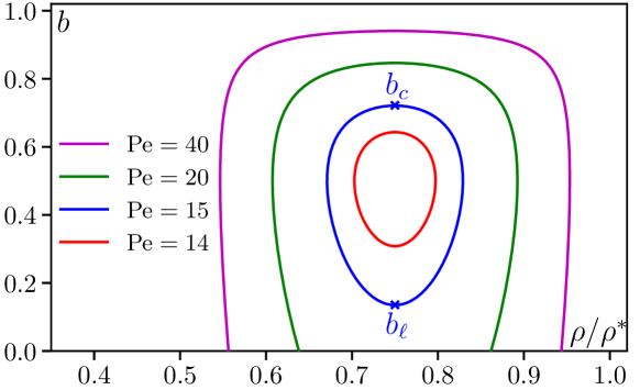
Figure 1: Evolution of the spinodal lines with Péclet number $\mathrm{Pe}$ in the continuum theory for overdamped biased MIPS, as described in Sec. 2.3.

The meeting of spinodal lines in a phase separation usually signal a critical point. At $\mathrm{Pe}=16$, the lower threshold $b_{\ell}=0$ corresponds to the critical point of unbiased MIPS which, in $d=2$, has been measured to be in the Ising universality class [37], although with conflicting reports [38]. Here we uncover a second critical point at $b_{c}$ which may be destroyed by fluctuations in $d=1$ but that we expect to survive in higher dimensions. Whether it would be in the same universality class as the critical point of unbiased MIPS is an interesting open problem.

2.4 Phase separation

As in MIPS, the instability identified in Sec. 2.3 signals a phase separation between dense and dilute phases. However, a striking difference with MIPS is that, because of the bias, the dense phase appears to be moving. Indeed, as shown by Eq. (20), there is a particle current $J_{0}(\rho)=\varepsilon\rho u(\rho)$ in a homogeneous phase at density $\rho$ which needs not be the same in both phases. One can then deduce the speed $c$ at which the dense phase is moving from a simple mass balance giving

$$c=\frac{J_{0}(\rho_{\ell})-J_{0}(\rho_{g})}{\rho_{\ell}-\rho_{g}}$$ (31)

with $\rho_{g}$ and $\rho_{\ell}$ the densities in the gas and liquid phases respectively.

In the unbiased case, the coexisting densities can be computed analytically using effective thermodynamic relations [15, 16]. However, when $b>0$, the additional gradient terms of even order in Eq. (15) invalidate this approach so that the coexisting densities need to be determined numerically. We do this for the linear velocity Eq. (4) both in numerical integration of the field theory Eq. (15) using a semi-spectral integration scheme with explicit time stepping and in simulations of the microscopic model Eq. (1) using parallel updates and Euler time stepping. The result is shown as a phase diagram in Fig. 2 along with density profiles. We see a good qualitative agreement between the microscopic simulations and the continuum description although with quantitative differences, especially in the gas binodal. In all our simulations, we find that $\rho_{\ell}>\rho^{*}$ so that the particles are not moving in the dense phase. The velocity $c$ of the dense phase given by Eq. (31) then reduces to $c=-\rho_{g}u(\rho_{g})/(\rho_{\ell}-\rho_{g})$ and is thus always negative so that the dense phase is moving upstream like traffic jams [2] or the freezed flocks of colloidal rollers of Ref. [39] which have a similar phenomenology.

Figure 2: Left: Phase diagram of the overdamped biased MIPS model computed in simulations of the PDE (15) and of the microscopic model Eq. (1). Right: instantaneous density profiles for $b=0.6$. Parameters: $u_{0}=2$, $D=0.1$, $\alpha=1$ (giving $\mathrm{Pe}=40$), $\rho^{*}=200$, mean density $\rho_{0}=0.7\rho^{*}$. $dt=0.005$ and $dx=0.5$ in integration of the PDE. $dt=0.1$ in integration of the microscopic model.

In Fig. 2 (left), we see that the gas binodal measured in the PDE appears to meet the spinodal before the critical point, at a lower value of $b$. This is not a numerical artefact and actually signals a transition from phase separation to microphase separation at higher $b$ values. We will discuss this phenomenon in more details in Sec. 3 where this transition happens further away from the critical point and is also observed in the microscopic model.

Note that even if we observe phase-separated profiles in microscopic simulations as shown in Fig. 2 (right), we do not expect it to be the asymptotic steady state in dimension $d=1$. Indeed, as in the 1d Ising model, there is no surface tension giving rise to a coarsening so that we expect domains of finite size in the thermodynamic limit. Here, in order to observe large domains to be able to measure binodals, we start from an initially phase-separated state with different densities and use large values of $\rho^{*}$ to effectively reduce fluctuations.

As we have seen, in the limit $b=1$ that is relevant to traffic flow, homogeneous profiles are always stable, at odds with traffic models [38, 29] in which, at high enough car density, a homogeneous car flow in unstable, leading to traffic jam. As we show in the next section, to recover this phenomenology, one needs to include inertial effects.

3 Traffic-flow scenario: fully biased dynamics with inertia

3.1 Definition of the model

We now consider an underdamped version of the model of Sec. 2 in the fully biased $b=1$ case. It can be seen as a minimal model of traffic flow on a highway, that is a long homogeneous portion of road with no crossing or traffic light. A given car $i$ is characterized by its (one-dimensional) position $x_{i}(t)$ at time $t$ on the road, and by its velocity $v_{i}(t)=dx_{i}/dt$. The car $i$ has a preferred velocity $u(\tilde{\rho}(x_{i}))$ that is computed in the same way as the quorum-sensing velocity of Sec. 2, using the kernel in Eq. (5) to compute the local density $\tilde{\rho}(x_{i})$. An important effect often taken into account in the traffic flow modelling literature is the fact that drivers take into account the density of cars in front of them, but not the density of cars behind [29, 24]. Hence strictly speaking, $\tilde{\rho}(x_{i})$ should be a measure of the density of cars just in front of car $i$. For the sake of simplicity, we neglect this effect here because it turns out to be inessential when discussing the analogy with MIPS.

We assume that the velocity relaxes to the preferred speed $u(\tilde{\rho})$ with a relaxation rate $\gamma$ (and relaxation time $\tau=\gamma^{-1}$), and is also subjected to an additive noise $\xi_{i}(t)$,

$$\frac{dv_{i}}{dt}=-\gamma\big{[}v_{i}-u\big{(}\tilde{\rho}(x_{i})\big{)}\big{]}+\gamma\sqrt{2D}\xi_{i}(t).$$ (32)

The functional dependence of the target speed $u(\tilde{\rho})$ is identical for all cars. In simulations we use the same linear dependence Eq. (4) which reproduces the non-monotonic variation of the car flow with density captured in the “fundamental diagram of traffic flow” [33]. The white noise $\xi_{i}(t)$ has the same correlation as in Eq. (3). In the overdamped limit $\gamma\to\infty$, we exactly recover the model of Sec. 2 with $b=1$.

3.2 Hydrodynamic equations

We introduce the single car phase-space distribution $f(x,v,t)$, defined as the probability density that a car with velocity $v$ is at position $x$ at time $t$. Using the same local mean-field approximation as in Sec. 2, we assume that $f(x,v,t)$ is not correlated with $\tilde{\rho}$ so that the distribution $f(x,v,t)$ obeys the following Fokker-Planck equation

$$\partial_{t}f+\partial_{x}\big{(}vf\big{)}-\gamma\partial_{v}\big{[}\big{(}v-u(\tilde{\rho})\big{)}f\big{]}=\gamma^{2}D\partial_{v}^{2}f.$$ (33)

The density field $\rho(x)$ and the car flux field $w(x)$ are connected to the phase-space distribution $f(x,v,t)$ through the relations

$$\rho(x,t)=\int_{-\infty}^{\infty}dv\,f(x,v,t),\qquad w(x,t)=\int_{-\infty}^{\infty}dv\,v\,f(x,v,t).$$ (34)

In these notations, the local average velocity is equal to $w/\rho$. Integrating Eq. (33) over the velocity $v$, an evolution equation for $\rho$ (the continuity equation) is obtained,

$$\partial_{t}\rho+\partial_{x}w=0.$$ (35)

An evolution equation for $w$ is also needed. We multiply Eq. (33) by $v$ and then integrate it over $v$, leading after integrations by part to:

$$\partial_{t}w+\partial_{x}S+\gamma\left(w-\rho u(\tilde{\rho})\right)=0,$$ (36)

where we have introduced the second moment in $v$ of the distribution $f$,

$$S(x,t)=\int_{-\infty}^{\infty}v^{2}f(x,v,t)\,dv.$$ (37)

Our goal is to expand Eq. (35) to drift-diffusion order, that is, to second order in gradients. We thus need to express $w$ in terms of $\rho$ to first order in gradients. For time scales larger than $\gamma^{-1}$, we can neglect the time derivative $\partial_{t}w$ in Eq. (36) since $w$ is a fast variable, and we get

$$w=\rho\tilde{u}-\frac{1}{\gamma}\partial_{x}S,$$ (38)

with again $\tilde{u}=u(\tilde{\rho})$. We thus need to obtain $S$ to zeroth order in gradient. At this order, we get from Eq. (33) the evolution equation for $S$,

$$\partial_{t}S+2\gamma(S-\tilde{u}w)=2\gamma^{2}D\rho.$$ (39)

For time scales larger than $\tau=\gamma^{-1}$, we can again neglect the time derivative, yielding

$$S=\tilde{u}w+\gamma D\rho.$$ (40)

At the same order of approximation, we have from Eq. (38) that $w=\tilde{u}\rho$, so that

$$S=\tilde{u}^{2}\rho+\gamma D\rho.$$ (41)

Eq. (38) can then be rewritten to first order in gradient as

$$w=\rho\tilde{u}-\frac{1}{\gamma}\partial_{x}\big{(}\rho\tilde{u}^{2}\big{)}-D\partial_{x}\rho.$$ (42)

Replacing $w$ in Eq. (35) by its expression (42), one eventually obtains a closed evolution equation on the density field $\rho$,

$$\partial_{t}\rho=-\partial_{x}\left(\rho\tilde{u}-2\tau\rho\tilde{u}\partial_{x}\tilde{u}\right)+\partial_{x}\left[\left(\tau\tilde{u}^{2}+D\right)\partial_{x}\rho\right].$$ (43)

We expand $\tilde{u}\equiv u(\tilde{\rho})$ as in Eq. (17) to get a fully explicit evolution equation for $\rho$. Eq. (43) then takes the form $\partial_{t}\rho=-\partial_{x}J$ with a particle current $J$ given by

$$J=J_{0}(\rho)-D_{\mathrm{eff}}(\rho)\partial_{x}\rho+m(\rho)\partial_{x}^{2}\rho+\Gamma_{1}\partial_{x}^{3}\rho-\Gamma_{2}\partial_{x}\rho\,\partial_{x}^{2}\rho$$ (44)

where $J_{0}(\rho)=\rho u$ as in Eq. (20), and the other coefficients are defined as

$$D_{\mathrm{eff}}(\rho) = D+\tau(\rho u^{2})^{\prime},$$ (45)

$$m(\rho) = \kappa\rho u^{\prime},$$ (46)

$$\Gamma_{1}(\rho) = -2\tau\kappa\rho uu^{\prime},$$ (47)

$$\Gamma_{2}(\rho) = 2\tau\kappa[\rho(uu^{\prime\prime}+u^{\prime 2})+uu^{\prime}].$$ (48)

3.3 Linear instability of the homogeneous car flow

Traffic congestion may be interpreted as resulting from the linear instability of an homogeneous car flow. We thus linearize Eq. (43) around the homogeneous state of density $\rho=\rho_{0}$, setting $\rho(x,t)=\rho_{0}+\delta\rho(x,t)$, which yields to first order in $\delta\rho$

$$\partial_{t}\delta\rho=-J_{0}^{\prime}(\rho_{0})\partial_{x}\delta\rho+D_{\mathrm{eff}}(\rho_{0})\partial_{x}^{2}\delta\rho-m(\rho_{0})\partial_{x}^{3}\delta\rho-\Gamma_{1}(\rho_{0})\partial_{x}^{4}\delta\rho.$$ (49)

The linear stability of the homogeneous state is determined by the sign of the effective diffusion coefficient $D_{\rm eff}(\rho_{0})$ defined in Eq. (45). When $u(\rho_{0})$ decreases fast enough, $D_{\rm eff}(\rho_{0})$ can become negative, signaling the instability of the homogeneous profile. In this case finite-wavelength perturbations grow exponentially in time for $q<q^{*}=\sqrt{|D_{\mathrm{eff}}(\rho_{0})|/\Gamma_{1}(\rho_{0})}$ (large $q$ perturbations are stabilized by the $q^{4}$ term).

The condition $D_{\mathrm{eff}}=0$ defines the spinodal line $\gamma_{s}(\rho_{0})$ with

$$\gamma_{s}=-\frac{(\rho u^{2})^{\prime}(\rho_{0})}{D}.$$ (50)

For the linear velocity dependence Eq. (4), Eq. (50) gives a critical $\gamma_{c}=u_{0}^{2}/(3D)$ below which the system is unstable in the density range between the spinodal lines

$$\rho_{s}^{\pm}=\frac{\rho^{*}}{3}\left[2\pm\sqrt{1-\frac{\gamma}{\gamma_{c}}}\right].$$ (51)

3.4 Phase separation

Fig. 3 shows the phase diagram in the $\gamma-\rho$ plane as determined in the continuum theory Eq. (43) and in the microscopic model. Let us first discuss that obtained from the PDE. It is markedly different from the usual phase diagram of a liquid-gas transition. In particular, we see that the lower binodal measured in simulations of the PDE encounters the spinodal line at $\gamma\approx 5.5$. For larger $\gamma$, phase separation is then impossible since the gas phase would be unstable. As shown in the snapshots, one then observes a microphase separation with an extensive number of high and low density domains. The amplitude of the oscillation decreases as $\gamma$ increases and vanishes at the critical point $\gamma_{c}$. Note that for $\gamma=7$, the solution shown in Fig. 3 is not periodic but we expect that adding a noise term to Eq. (15) would allow the periodic solutions to be reached, as is the case for the microphase separation in flocking models [40].

Compared to a passive liquid-gas phase separation or the usual MIPS, the transition between phase and microphase separation is made possible by the nonlinear drift term $J_{0}(\rho)$ in Eq. (15). Indeed, this term does not affect the spinodals that are controlled by $D_{\rm eff}$, but it does affect the binodals. In contrast, for a conventional phase separation both the binodals and spinodals are controlled by the free energy (or effective free energy for MIPS [15]), and thus cannot cross. The same physics is captured in a minimal setting by the convective Cahn-Hilliard equation [34] in which a convective non-linearity (that would enter in our notation as $J_{0}\propto\rho^{2}$) is added to the standard Cahn-Hilliard equation.

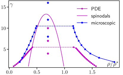
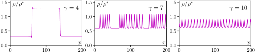
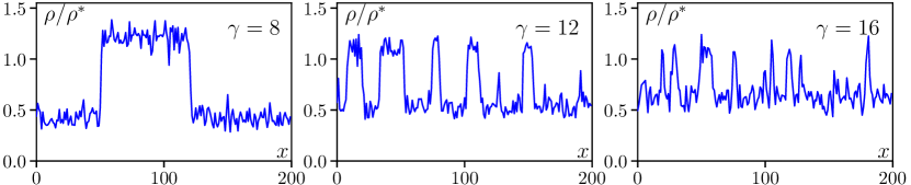
Figure 3: Top: Phase diagram of the traffic model computed in simulations of the PDE (43) and of the microscopic model Eq. (32). For the PDE, the spinodals correspond to the limit of linear stability of homogeneous profiles given by Eq. (51). The binodals are measured in the PDE and microscopic model as the coexisting densities of phase separated profiles which exist below the dashed lines. The stars indicate the parameters of the snapshots shown below. Middle row: Snapshots from numerical integration of the PDE starting from a phase separated initial condition. Bottom: Snapshots from simulations of the microscopic model starting from a phase separated initial condition. Parameters: $D=1$, $u_{0}=2$, $\rho^{*}=200$, $\rho_{0}=0.7\rho^{*}$, system size $L=200$. $dt=0.005$ and $dx=0.5$ for the PDE. $dt=0.1$ for the microscopic model.

Comparing the phase diagrams from the PDE and microscopic model, we see that quantitatively the agreement is rather poor which could be explained by the additional large $\gamma$ (or small $\tau$) approximation that was needed compared to the overdamped case of Sec. 2. However, qualitatively, the same phenomenon is observed: a phase separation at low values of $\gamma$ crossing over to a microphase separation at larger $\gamma$ with domains of decreasing amplitude as $\gamma$ increases, as shown in the snapshots of Fig. 3 (bottom).

4 Bridging MIPS and congested flow: inertial dynamics with tumbles

We have seen that the overdamped fully biased dynamics lead to a stable homogeneous state. Phase separation is recovered either by decreasing the bias (leading to MIPS) or by reintroducing inertia, with a damping coefficient below a threshold value (leading to traffic jams). In this perspective, MIPS and traffic jam seemingly appear as disconnected phenomena, present in different parts of the phase diagram of the model, and related to distinct physical ingredients. However, a definite conclusion can only be reached by considering the two-dimensional phase diagram in the parameter plane $(b,\tau$), with $\tau=\gamma^{-1}$ the speed relaxation time, rather than only the parameter lines $(b,\tau=0)$ [Section 2] and $(b=1,\tau)$ [Section 3] separately.

4.1 Model with inertial dynamics and biased tumbling rates

We combine the underdamped model of Sec. 3 with the biased tumbling dynamics of Sec. 2. The velocity $v_{i}$ evolves according to

$$\frac{dv_{i}}{dt}=-\gamma\big{[}v_{i}-u(\tilde{\rho})e_{i}(t)\big{]}+\gamma\sqrt{2D}\xi_{i}(t)$$ (52)

where $e_{i}(t)$ has the same dynamics as in Sec. 2, and the white noise $\xi_{i}(t)$ has the correlation Eq. (3).

4.2 Hydrodynamic description

The derivation of the hydrodynamic equation follows the techniques of Sec. 2 and 3 combined. Let us introduce the phase space densities $f_{+}(x,v,t)$ and $f_{-}(x,v,t)$ describing the probability densities to find a particle at position $x$ with velocity $v$ with $e_{i}=1$ or $e_{i}=-1$ respectively. The densities $f_{+}$ and $f_{-}$ evolve according to

$$\!\!\!\!\!\!\!\!\partial_{t}f_{+}+\partial_{x}\big{(}vf_{+}\big{)}-\gamma\partial_{v}\left[(v-\tilde{u})f_{+}\right] = \gamma^{2}D\partial_{v}^{2}f_{+}-\alpha(1-b)f_{+}+\alpha f_{-},$$ (53)

$$\!\!\!\!\!\!\!\!\partial_{t}f_{-}+\partial_{x}\big{(}vf_{-}\big{)}-\gamma\partial_{v}\left[(v+\tilde{u})f_{-}\right] = \gamma^{2}D\partial_{v}^{2}f_{-}-\alpha f_{-}+\alpha(1-b)f_{+},$$ (54)

with again the shorthand notation $\tilde{u}=u(\tilde{\rho})$. It is convenient to introduce the total phase space density $f=f_{+}+f_{-}$, as well as $g=f_{-}-(1-b)f_{+}$, by analogy with Sec. 2. Keeping the same notations, we have

$$\partial_{t}f + \partial_{x}\big{(}vf\big{)}-\gamma\partial_{v}\left[(v-\varepsilon\tilde{u})f\right]-(1+\varepsilon)\gamma\partial_{v}(\tilde{u}g)=\gamma^{2}D\partial_{v}^{2}f,$$ (55)

$$\partial_{t}g + \partial_{x}\big{(}vg\big{)}-\gamma\partial_{v}\left[(v+\varepsilon\tilde{u})g\right]-\mu\gamma\partial_{v}(\tilde{u}f)=\gamma^{2}D\partial_{v}^{2}g-\tilde{\alpha}g,$$ (56)

with $\mu=2(1-b)/(2-b)$ and $\tilde{\alpha}=\alpha(2-b)$. We use the fields $\rho(x,t)$, $w(x,t)$ and $S(x,t)$ defined as the first moments in $v$ of the phase space distribution $f(x,v,t)$ as in Eqs. (34) and (37). Similarly, we also introduce the following auxiliary fields related to the function $g(x,v,t)$:

$$q(x,t) = \int_{-\infty}^{\infty}g(x,v,t)\,dv,$$ (57)

$$\bar{w}(x,t) = \int_{-\infty}^{\infty}v\,g(x,v,t)\,dv,$$ (58)

$$\bar{S}(x,t) = \int_{-\infty}^{\infty}v^{2}g(x,v,t)\,dv.$$ (59)

Integrating Eq. (55) over $v$, one finds the evolution equation for $\rho$, which reads

$$\partial_{t}\rho=-\partial_{x}w,$$ (60)

so that we need to evaluate $w$ at first order in gradients. We apply a similar method as in the previous cases, by determining the evolution equation for the successive low-order moments of $f$ and $g$. Typically, the evolution equation of the moment of order $n$ involves a gradient of the moment of order $n+1$, successively leading to truncations at lower and lower order in the gradient expansion. In addition, moments of order $n>0$ can be considered as fast variables and their time derivative can be neglected after a coarse-graining in time. These approximations allow us to truncate and close the moment hierarchy at order $n=2$. A detailed derivation is given in A. We eventually obtain an explicit expression for $w$,

$$w=\big{[}\varepsilon\tilde{u}-\eta(\tilde{u}\partial_{x}\tilde{u})\big{]}\rho-\big{[}\tilde{\eta}\tilde{u}^{2}+D\big{]}\partial_{x}\rho,$$ (61)

with

$$\zeta = \frac{4(1-b)\beta\gamma}{(2-b)^{2}},$$ (62)

$$\eta = \frac{\zeta}{\tilde{\alpha}}+\frac{2}{\gamma}(\varepsilon^{2}+\zeta),$$ (63)

$$\tilde{\eta} = \frac{\zeta}{\tilde{\alpha}}+\frac{1}{\gamma}(\varepsilon^{2}+\zeta).$$ (64)

From Eq. (60), we finally get a closed evolution equation for $\rho$,

$$\partial_{t}\rho=-\partial_{x}\big{(}\varepsilon\rho\tilde{u}-\eta\rho\tilde{u}\partial_{x}\tilde{u}\big{)}+\partial_{x}\left[\big{(}\tilde{\eta}\tilde{u}^{2}+D\big{)}\partial_{x}\rho\right].$$ (65)

A more explicit expression of $\eta$ and $\tilde{\eta}$ is obtained by expanding these coefficients to leading order in the relaxation time $\tau=\gamma^{-1}$, for $\tau\to 0$:

$$\eta = \frac{4(1-b)}{\alpha(2-b)^{3}}+2\tau\,\frac{1+(1-b)^{2}}{(2-b)^{2}},$$ (66)

$$\tilde{\eta} = \frac{4(1-b)}{\alpha(2-b)^{3}}+\tau\,\frac{b^{2}}{(2-b)^{2}}.$$ (67)

These expressions match the results of the previous sections. For $\tau=0$ (overdamped dynamics), one recovers $\eta=\eta^{\prime}=\eta_{0}$ in agreement with Eq. (16), while for $b=1$, one recovers $\eta=2\tau$ and $\eta^{\prime}=\tau$ consistently with Eq. (43).

We expand $\tilde{u}\equiv u(\tilde{\rho})$ as in Eq. (17) to get a fully explicit evolution equation for $\rho$. Eq. (65) then takes the form $\partial_{t}\rho=-\partial_{x}J$ with a particle current $J$ given by

$$J=J_{0}(\rho)-D_{\mathrm{eff}}(\rho)\partial_{x}\rho+m(\rho)\partial_{x}^{2}\rho+\Gamma_{1}(\rho)\partial_{x}^{3}\rho-\Gamma_{2}(\rho)\partial_{x}\rho\,\partial_{x}^{2}\rho$$ (68)

with again the same current $J_{0}(\rho)=\varepsilon\rho u(\rho)$, and where

$$D_{\mathrm{eff}}(\rho) = D+\eta\rho uu^{\prime}+\tilde{\eta}u^{2},$$ (69)

$$m(\rho) = \kappa\varepsilon\rho u^{\prime},$$ (70)

$$\Gamma_{1}(\rho) = -\eta\kappa\rho uu^{\prime},$$ (71)

$$\Gamma_{2}(\rho) = \eta\kappa\rho(uu^{\prime\prime}+u^{\prime 2})+2\tilde{\eta}\kappa uu^{\prime}.$$ (72)

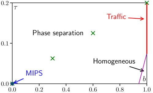
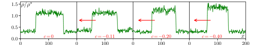
Figure 4: Phase diagram in the $(b,\tau)$-plane of the bias $b$ and relaxation time $\tau$. The purple line delimit the regions where only homogeneous states are observed at high $b$ and small $\tau$ and the region where phase separation is observed for a range of densities. The green crosses indicate the position of the snapshots shown in the lower panel. They show that one can continuously change parameters from the unbiased MIPS (blue dot) to the (micro) phase separation seen in the fully-biased traffic model of Sec. 3. The red arrows emphasize the motion of the dense phase at the indicated speed $c$. Parameters: system size $L=200$, $\rho^{*}=200$, $\rho_{0}=0.7\rho^{*}$, $u_{0}=2$, $D=0.1$, corresponding to $\mathrm{Pe}=40$.

4.3 Linear stability analysis

We linearize Eq. (65) around the homogeneous state of density $\rho=\rho_{0}$, setting $\rho(x,t)=\rho_{0}+\delta\rho(x,t)$, which yields to first order in $\delta\rho$

$$\partial_{t}\delta\rho=-J_{0}^{\prime}(\rho_{0})\partial_{x}\delta\rho+D_{\mathrm{eff}}(\rho_{0})\partial_{x}^{2}\delta\rho-m(\rho_{0})\partial_{x}^{3}\delta\rho-\Gamma_{1}(\rho_{0})\partial_{x}^{4}\delta\rho,$$ (73)

As before the homogeneous state may become linearly unstable when $D_{\mathrm{eff}}<0$, in which case the instability occurs for small wave-vectors $q<q^{*}=\sqrt{|D_{\mathrm{eff}}(\rho_{0})|/\Gamma_{1}(\rho_{0})}$.

In Fig. 4, we plot the phase diagram in the $(b,\tau)$ plane computed from the condition $D_{\mathrm{eff}}<0$ for a fixed Péclet number $\mathrm{Pe}=u_{0}^{2}/(\alpha D)=40$. The purple line separates a region at small $\tau$ and large $b$ in which homogeneous profiles are stable at any density (and phase separation is thus never observed) from a region where phase separation is observed is some density range. From that plot, it is clear that the phase separation seen in unbiased MIPS ($b=0$, $\tau=0$) is continuously connected to the traffic congestion ($b=1$, $\tau>0$). The snapshots shown in Fig. 4 (bottom) confirm that, indeed, such a continuous interpolation also exists in the microscopic model.

It is interesting to see how the phase diagram evolves with Péclet number. As shown in Fig. 5, we see that at lower activity it becomes non-monotonous. Below the critical value $\mathrm{Pe}=27/2$ already identified in Sec. 2.3, inertia is necessary to observe phase separation. More generally, we find that contrary to what is seen in models of self-propelled disks [26], inertia always has a destabilizing effect on homogeneous profiles and thus promotes MIPS. The snapshots in Fig. 5 confirm that, even for $b=0$, this stabilization of MIPS by inertia also happens in the microscopic model.

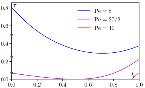
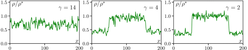
Figure 5: Top: Phase diagram in the $(b,\tau)$-plane, as in Fig. 4, for several values of $\mathrm{Pe}=u_{0}^{2}/(\alpha D)$. The green stars indicate the position of the snapshots shown below. Bottom: Snapshots from the microscopic model in the unbiased case $b=0$ at $\mathrm{Pe}=16$ ($u_{0}=2$, $\alpha=1$, $D=0.25$) showing that MIPS can be observed only when inertia is strong enough (i.e. large $\tau$/small $\gamma$).

5 Conclusion

In this paper we have introduced and studied a one-dimensional model featuring run-and-tumble particles with tumbles that are biased in one direction. They interact via a target speed $u(\rho)$ that is a decreasing function of the local density and to which the particles relax at a finite rate $\gamma$. In Sec. 2, we first considered the case of overdamped particles with biased tumbles which could describe systems showing MIPS in presence of an external bias such as chemotaxis toward a food source for bacteria. We then considered in Sec. 3 the completely biased overdamped case which is most naturally interpreted as a traffic model on a highway showing traffic jams. Finally, in Sec. 4 we have put both ingredients together to look at the phase diagram in terms of both the bias and relaxation rate. In the three cases, we have derived the hydrodynamic equation for the density field and used it to study the linear stability of homogeneous profiles. We then compared the phase diagrams obtained with numerical simulations of the microscopic model and of the continuum equations.

Let us recapitulate the most salient features observed in our model. (i) We find that the “usual” (overdamped unbiased) MIPS survives the addition of bias, with an ordered phase moving against the flow of particles. However, MIPS is lost at any activity level at large values of the bias. (ii) Inertia promotes phase separation and restores it in the fully biased case. Even in the unbiased case, MIPS can be observed in presence of inertia for activity levels such that it is absent in the overdamped case. (iii) The full model allows us to show that MIPS and the traffic jams seen in the fully biased model are essentially the same phenomenon as one can go continuously from one to the other. (iv) For some parameter values, we observe that inhomogeneous profiles transition from phase separation to microphase separation. This happens when a binodal line crosses the spinodal line so that a macroscopic phase coexistence becomes unstable. Such a phenomenon, studied before in the context of a convective Cahn-Hilliard equation [34], is made possible here by the bias which generates terms of odd order in gradient in the continuous description.

In the microscopic model, the study of the phase to microphase separation transition is complicated by the fact that, in one dimension, fluctuations are already expected to break a macroscopic phase separation into an extensive number of domains. We circumvented this difficulty by considering large densities in order to reduce fluctuations. However, we expect our results to extend to higher dimensions, as long as the bias remains along one preferred direction, in which case the transition will be more easily studied. Whether this transition can happen for any value of the bias or only beyond a critical bias remains an open question left for future work. In addition, considering the higher dimensional case would allow one to assess the universality class of the critical point of the phase (or microphase) separation at non-zero bias. Finally, our model builds on the quorum-sensing model of MIPS which is well described by the active model B [41], showing macroscopic phase separation and a positive surface tension. It could be interesting to study a biased version of self-propelled disks which fall in the class of active model B+ [42] showing negative surface tension [14, 16] and a bubbly phase separation [43, 17]. A potential additional instability of the phase separation due to the bias, as we observe, could lead to a very rich phenomenology.

Acknowledgements.

We thank Hugues Chaté for useful discussions.

Appendix A Evaluation of $w$ for the inertial dynamics with tumbles

We evaluate the field $w$ using a gradient expansion to second order of the evolution equations for the low-order moments of $f$ and $g$. Multiplying Eq. (55) by $v$ and integrating over $v$, we get after an integration by part

$$\partial_{t}w+\partial_{x}S+\gamma(w-\varepsilon\tilde{u}\rho)+(1+\varepsilon)\gamma\tilde{u}q=0.$$ (74)

On time scales much larger than $\tau=\gamma^{-1}$, we can neglect $\partial_{t}w$, leading to

$$w=\varepsilon\tilde{u}\rho-(1+\varepsilon)\tilde{u}q-\frac{1}{\gamma}\partial_{x}S.$$ (75)

To obtain $w$, we thus need to determine $q$ to first order in gradient, and $S$ to zeroth order in gradient. Integrating Eq. (56) over $v$, we get

$$\partial_{t}q+\partial_{x}\bar{w}=-\tilde{\alpha}q.$$ (76)

On time scales much larger than $\alpha^{-1}$, we thus get

$$q=-\frac{1}{\tilde{\alpha}}\partial_{x}\,\bar{w}.$$ (77)

It follows that we need to determine $\bar{w}$ at zeroth order in gradient. Multiplying Eq. (56) by $v$ and integrating over $v$, we get after an integration by part,

$$\partial_{t}\bar{w}+\partial_{x}\bar{S}+\gamma\varepsilon\tilde{u}q+(1+\varepsilon)(1-b)\gamma\tilde{u}\rho=-(\gamma+\tilde{\alpha})\bar{w}.$$ (78)

Neglecting time and space derivatives and taking into account Eq. (77) to neglect the term proportional to $q$, the expression of $\bar{w}$ simplified to

$$\bar{w}=-(1+\varepsilon)(1-b)\beta\gamma\,\tilde{u}\rho$$ (79)

where we have introduced $\beta=(\gamma+\tilde{\alpha})^{-1}$. It follows from Eqs. (77) and (79) that

$$q=(1+\varepsilon)\frac{(1-b)\beta\gamma}{\tilde{\alpha}}\,\partial_{x}(\tilde{u}\rho).$$ (80)

We now determine $S$ to zeroth order in gradient. Multiplying Eq. (55) by $v^{2}$ and integrating over $v$, we get after integration by part and neglected gradient terms

$$\partial_{t}S+2\gamma(S-\varepsilon\tilde{u}w)+2\gamma(1+\varepsilon)\,\tilde{u}\bar{w}=2\gamma^{2}D\rho.$$ (81)

Neglecting the time derivative $\partial_{t}S$ since $S$ is a fast field and using respectively the expressions (75) and (79) of $w$ and $\bar{w}$ to zeroth order in gradient, we get

$$S=(\varepsilon^{2}+\zeta)\tilde{u}^{2}\rho+\gamma D\rho$$ (82)

with

$$\zeta=\frac{4(1-b)\beta\gamma}{(2-b)^{2}}.$$ (83)

Plugging the expressions (80) of $q$ and (82) of $S$ into Eq. (75), we finally obtain Eq. (61) for the expression of $w$.

References

- [1] Boris S Kerner and Hubert Rehborn. Experimental properties of phase transitions in traffic flow. Physical Review Letters 79, 4030 (1997). Publisher: APS.
- [2] Boris S. Kerner. Experimental features of self-organization in traffic flow. Physical review letters 81, 3797 (1998). Publisher: APS.
- [3] Boris S Kerner and Hubert Rehborn. Experimental features and characteristics of traffic jams. Physical Review E 53, R1297 (1996). Publisher: APS.
- [4] Fred L Hall, Brian L Allen, and Margot A Gunter. Empirical analysis of freeway flow-density relationships. Transportation Research Part A: General 20, 197 (1986). Publisher: Elsevier.
- [5] Lutz Neubert, Ludger Santen, Andreas Schadschneider, and Michael Schreckenberg. Single-vehicle data of highway traffic: A statistical analysis. Physical Review E 60, 6480 (1999). Publisher: APS.
- [6] J. Tailleur and M. E. Cates. Statistical mechanics of interacting run-and-tumble bacteria. Physical review letters 100, 218103 (2008).
- [7] Michael E. Cates and Julien Tailleur. Motility-Induced Phase Separation. Annual Review of Condensed Matter Physics 6, 219 (2015).
- [8] Jérémy O’Byrne, Alexandre Solon, Julien Tailleur, and Yongfeng Zhao. An Introduction to Motility-induced Phase Separation. In Out-of-equilibrium Soft Matter pages 107. The Royal Society of Chemistry 2023.
- [9] Xiongfei Fu, Lei-Han Tang, Chenli Liu, Jian-Dong Huang, Terence Hwa, and Peter Lenz. Stripe formation in bacterial systems with density-suppressed motility. Physical review letters 108, 198102 (2012).
- [10] Guannan Liu, Adam Patch, Fatmagül Bahar, David Yllanes, Roy D Welch, M Cristina Marchetti, Shashi Thutupalli, and Joshua W Shaevitz. Self-Driven Phase Transitions Drive Myxococcus xanthus Fruiting Body Formation. Physical review letters 122, 248102 (2019). Publisher: APS.
- [11] AI Curatolo, N Zhou, Y Zhao, C Liu, A Daerr, J Tailleur, and J Huang. Cooperative pattern formation in multi-component bacterial systems through reciprocal motility regulation. Nature Physics 16, 1152 (2020). Publisher: Nature Publishing Group UK London.
- [12] Caleb Anderson and Alberto Fernandez-Nieves. Social interactions lead to motility-induced phase separation in fire ants. Nature Communications 13, 6710 (2022). Publisher: Nature Publishing Group UK London.
- [13] Tobias Bäuerle, Andreas Fischer, Thomas Speck, and Clemens Bechinger. Self-organization of active particles by quorum sensing rules. Nature communications 9, 1 (2018). Publisher: Nature Publishing Group.
- [14] Julian Bialké, Jonathan T Siebert, Hartmut Löwen, and Thomas Speck. Negative interfacial tension in phase-separated active Brownian particles. Physical review letters 115, 098301 (2015). Publisher: APS.
- [15] Alexandre P. Solon, Joakim Stenhammar, Michael E. Cates, Yariv Kafri, and Julien Tailleur. Generalized thermodynamics of phase equilibria in scalar active matter. Phys. Rev. E 97, 020602 (2018).
- [16] Alexandre Solon, Joakim Stenhammar, Mike E Cates, Yariv Kafri, and Julien Tailleur. Generalized thermodynamics of motility-induced phase separation: phase equilibria, Laplace pressure, and change of ensembles. New Journal of Physics (2018).
- [17] Xia-qing Shi, Giordano Fausti, Hugues Chaté, Cesare Nardini, and Alexandre Solon. Self-Organized Critical Coexistence Phase in Repulsive Active Particles. Physical Review Letters 125, 168001 (2020). Publisher: APS.
- [18] Thomas Speck, Julian Bialké, Andreas M Menzel, and Hartmut Löwen. Effective Cahn-Hilliard equation for the phase separation of active Brownian particles. Physical Review Letters 112, 218304 (2014).
- [19] Yaouen Fily and M. Cristina Marchetti. Athermal phase separation of self-propelled particles with no alignment. Physical review letters 108, 235702 (2012).
- [20] Gabriel S. Redner, Michael F. Hagan, and Aparna Baskaran. Structure and dynamics of a phase-separating active colloidal fluid. Physical review letters 110, 055701 (2013).
- [21] Joakim Stenhammar, Adriano Tiribocchi, Rosalind J. Allen, Davide Marenduzzo, and Michael E. Cates. Continuum theory of phase separation kinetics for active brownian particles. Physical review letters 111, 145702 (2013).
- [22] Ivo Buttinoni, Julian Bialké, Felix Kümmel, Hartmut Löwen, Clemens Bechinger, and Thomas Speck. Dynamical clustering and phase separation in suspensions of self-propelled colloidal particles. Physical review letters 110, 238301 (2013).
- [23] Marjolein N Van Der Linden, Lachlan C Alexander, Dirk GAL Aarts, and Olivier Dauchot. Interrupted motility induced phase separation in aligning active colloids. Physical review letters 123, 098001 (2019). Publisher: APS.
- [24] Debashish Chowdhury, Ludger Santen, and Andreas Schadschneider. Statistical physics of vehicular traffic and some related systems. Physics Reports 329, 199 (2000). Publisher: Elsevier.
- [25] Antonio Suma, Giuseppe Gonnella, Davide Marenduzzo, and Enzo Orlandini. Motility-induced phase separation in an active dumbbell fluid. Europhysics Letters 108, 56004 (2014). Publisher: IOP Publishing.
- [26] Suvendu Mandal, Benno Liebchen, and Hartmut Löwen. Motility-induced temperature difference in coexisting phases. Physical Review Letters 123, 228001 (2019). Publisher: APS.
- [27] AP Solon, ME Cates, and J Tailleur. Active brownian particles and run-and-tumble particles: A comparative study. The European Physical Journal Special Topics 224, 1231 (2015).
- [28] Howard C. Berg and Douglas A. Brown. Chemotaxis in Escherichia coli analysed by three-dimensional tracking. Nature 239, 500 (1972).
- [29] Michael Schreckenberg, Andreas Schadschneider, Kai Nagel, and Nobuyasu Ito. Discrete stochastic models for traffic flow. Physical Review E 51, 2939 (1995). Publisher: APS.
- [30] Martin R Evans. Bose-Einstein condensation in disordered exclusion models and relation to traffic flow. Europhysics Letters 36, 13 (1996). Publisher: IOP Publishing.
- [31] Martin R Evans, Nikolaus Rajewsky, and Eugene R Speer. Exact solution of a cellular automaton for traffic. Journal of statistical physics 95, 45 (1999). Publisher: Springer.
- [32] AATM Aw and Michel Rascle. Resurrection of” second order” models of traffic flow. SIAM journal on applied mathematics 60, 916 (2000). Publisher: SIAM.
- [33] Florian Siebel and Wolfram Mauser. On the fundamental diagram of traffic flow. SIAM Journal on Applied Mathematics 66, 1150 (2006). Publisher: SIAM.
- [34] AA Golovin, AA Nepomnyashchy, Stephen H Davis, and MA Zaks. Convective Cahn-Hilliard models: From coarsening to roughening. Physical review letters 86, 1550 (2001). Publisher: APS.
- [35] Julian Bialké, Hartmut Löwen, and Thomas Speck. Microscopic theory for the phase separation of self-propelled repulsive disks. EPL (Europhysics Letters) 103, 30008 (2013).
- [36] Thibaut Arnoulx de Pirey, Gustavo Lozano, and Frédéric Van Wijland. Active hard spheres in infinitely many dimensions. Physical review letters 123, 260602 (2019). Publisher: APS.
- [37] Claudio Maggi, Matteo Paoluzzi, Andrea Crisanti, Emanuela Zaccarelli, and Nicoletta Gnan. Universality class of the motility-induced critical point in large scale off-lattice simulations of active particles. Soft Matter 17, 3807 (2021). Publisher: Royal Society of Chemistry.
- [38] Jonathan Tammo Siebert, Florian Dittrich, Friederike Schmid, Kurt Binder, Thomas Speck, and Peter Virnau. Critical behavior of active Brownian particles. Physical Review E 98, 030601 (2018). Publisher: APS.
- [39] Delphine Geyer, David Martin, Julien Tailleur, and Denis Bartolo. Freezing a flock: Motility-induced phase separation in polar active liquids. Physical Review X 9, 031043 (2019). Publisher: APS.
- [40] Alexandre P Solon, Jean-Baptiste Caussin, Denis Bartolo, Hugues Chaté, and Julien Tailleur. Pattern formation in flocking models: A hydrodynamic description. Physical Review E 92, 062111 (2015).
- [41] Raphael Wittkowski, Adriano Tiribocchi, Joakim Stenhammar, Rosalind J. Allen, Davide Marenduzzo, and Michael E. Cates. Scalar phi4 field theory for active-particle phase separation. Nature communications 5 (2014).
- [42] Elsen Tjhung, Cesare Nardini, and Michael E Cates. Cluster phases and bubbly phase separation in active fluids: Reversal of the ostwald process. Physical Review X 8, 031080 (2018). Publisher: APS.
- [43] Claudio B Caporusso, Pasquale Digregorio, Demian Levis, Leticia F Cugliandolo, and Giuseppe Gonnella. Motility-induced microphase and macrophase separation in a two-dimensional active Brownian particle system. Physical Review Letters 125, 178004 (2020). Publisher: APS.