Abstract

We present a consistent formalism to describe the dynamics of hybrid systems with mixed classical and quantum degrees of freedom. The probability function of the system, which, in general, will be a combination of the classical distribution function and the quantum density matrix, is described in terms of its corresponding moments. We then define a hybrid Poisson bracket, such that the dynamics of the moments is ruled by an effective Hamiltonian. In particular, a closed formula for the Poisson brackets between any two moments for an arbitrary number of degrees of freedom is presented, which corrects previous expressions derived in the literature for the purely quantum case. This formula is of special relevance for practical applications of the formalism. Finally, we study the dynamics of a particular hybrid system given by two coupled oscillators, one being quantum and the other classical. Due to the coupling, specific quantum and classical properties are transferred between different sectors. In particular, the quantum sector is allowed to violate the uncertainty relation, though we explicitly show that there exists a minimum positive bound of the total uncertainty of the hybrid system.

1 Introduction

The boundary between classical and quantum physics remains unknown. It is within this context that the exploration of hybrid classical-quantum physics has emerged, aiming to describe the interaction between genuinely classical and genuinely quantum systems. Certainly, this study can shed light on the aforementioned problem and, moreover, it is motivated by a variety of reasons, both practical and theoretical. For instance, in the Copenhagen interpretation of quantum mechanics, measuring devices are regarded as classical [1, 2, 3, 4]. Therefore, a comprehensive understanding of the coexistence of quantum and classical sectors is essential for this foundational interpretation. Furthermore, if one considers that gravity is fundamentally classical, hybrid classical-quantum physics can be essential to understand how it interacts with quantum systems [5, 6]. On the other hand, from a practical standpoint, in certain intricate quantum systems, considering some degrees of freedom as classical can be very useful in order to obtain a simpler approximate description of the dynamics. This is of particular relevance in fields like molecular or condensed matter physics [7, 8, 9, 10, 11, 12, 13], but it is also the main motivation to consider quantum field theory on classical curved backgrounds as a good approximation to a prospective full theory of quantum gravity.

Undoubtedly, these examples highlight the necessity for a hybrid theory. However, so far there is not a unique, perfect, construction, and several proposals can be found in the literature (for reviews on the different proposals we refer the reader to Refs. [14, 15]). These approaches exhibit a broad spectrum of methodologies. For example, some try to preserve the use of quantum states and trajectories to describe, respectively, the quantum and classical sectors [5, 16]. Moreover, some focus on a quantum formalism for the whole hybrid system, by formulating the classical sector as quantum [17, 18, 19, 20, 21, 22, 26, 27, 6, 23, 24, 25, 28, 29, 30]. Conversely, some others formulate the quantum sector in classical terms, in order to work with a formally complete classical system [31, 32, 33, 34, 35, 36]. Additionally, certain proposals bring the quantum and classical sectors into a common language, in order to extend it to the interacting hybrid system [37, 38, 39, 40]. It is also worth mentioning that some approaches begin by building a fully quantum system and then take a classical limit in one of the subsystems, in order to get a classical-quantum interacting system [41]. Nevertheless, all of them deal with some inconsistencies, such as the inability to define a Lie bracket, the nonpositivity of the probability distribution, an inconsistent classical limit, a nonunitary evolution, or the inability to distinguish between the classical and quantum sectors.

Hence, in this paper, we present a new proposal for a consistent description of the dynamics of hybrid systems, with a different starting point and formalism. It is motivated by a formalism for quantum systems that replaces the wave function (or more generally the density matrix), by its infinite set of moments [43, 42]. As analyzed in Refs. [43, 44], this approach can also be used to describe classical ensembles, and, thus, we propose a similar extension of the formalism to include hybrid systems. Such extension will rely on the definition of a bracket for hybrid observables, which will generalize the quantum commutator and the classical Poisson bracket.

The rest of the paper is organized as follows. In Sec. 2 the formalism for quantum systems is presented. As commented above, this is a well known formalism, though, as an original result, here we provide a closed formula for the Poisson bracket between moments for any number of degrees of freedom, which corrects the formula presented in Ref. [42]. In Sec. 3 we show that a similar formalism as presented for quantum systems can be used to describe the dynamics of classical ensembles. This generalizes the work of Refs. [43, 44] to an arbitrary number of degrees of freedom. In Sec. 4 we present the hybrid case, with mixed classical and quantum degrees of freedom, and, in particular, define the hybrid bracket that generalizes the quantum commutator and the classical Poisson bracket. Sec. 5 comments on the specific dynamical properties of harmonic Hamiltonians, defined as those that are at most quadratic on basic variables. Then, in Sec. 6 a particular application of the formalism is considered, and we study in detail the hybrid system given by a classical oscillator coupled to a quantum one. Finally, in Sec. 7 we present the conclusions and summarize the main results of the paper. There are two additional appendices with technical computations: in App. A we derive the main steps of the derivation of the formula for the Poisson bracket between moments, while in App. B the properties of the bracket between hybrid observables are analyzed.

2 Quantum Systems

Let us consider a system with $N$ quantum degrees of freedom described by the basic operators $(\hat{q}_{j},\hat{p}_{j})_{j=1}^{N}$, which obey the usual canonical commutation relations $[\hat{q}_{j},\hat{p}_{k}]=i\hbar\delta_{jk}$. The central moments of the wave function, or, more generically, of the density matrix, are defined as the expectation value

$$\Delta\big{(}q_{1}^{a_{1}}p_{1}^{b_{1}}\dots q_{N}^{a_{N}}p_{N}^{b_{N}}\big{)}:=\left\langle(\hat{q}_{1}-q_{1})^{a_{1}}(\hat{p}_{1}-p_{1})^{b_{1}}\dots(\hat{q}_{N}-q_{N})^{a_{N}}(\hat{p}_{N}-p_{N})^{b_{N}}\right\rangle_{\text{Weyl}},$$ (1)

for any nonnegative integers $a_{i}$, $b_{i}$. In this expression we have defined $q_{i}:=\langle\hat{q}_{i}\rangle$ and $p_{i}:=\langle\hat{p}_{i}\rangle$, while the subscript Weyl refers to a totally symmetric ordering of the basic operators. A priori one could choose another ordering for this definition but, with the present choice, one ensures that all the moments are real-valued time-dependent functions. Therefore, this definition can be understood as a decomposition of the density matrix of the system into an infinite set of variables, which only depend on time and represent the actual measurable quantities of the system.

In the Heisenberg picture the state of the system is described by a constant (time-independent) wave function (or density matrix), and the evolution of any operator $\hat{A}$ follows

$$\frac{d\hat{A}}{dt}=\frac{\partial\hat{A}}{\partial t}+\frac{1}{i\hbar}\left[\hat{A},\hat{H}\right],$$ (2)

where $\hat{H}$ is the Hamiltonian operator. Taking the expectation value of this expression, one obtains

$$\frac{d\langle\hat{A}\rangle}{dt}=\bigg{\langle}\frac{\partial\hat{A}}{\partial t}\bigg{\rangle}+\frac{1}{i\hbar}\left\langle\left[\hat{A},\hat{H}\right]\right\rangle.$$ (3)

Therefore, defining the Poisson bracket between expectation values as $\{\langle\hat{f}\rangle,\langle\hat{g}\rangle\}:=-i\hbar^{-1}\langle[\hat{f},\hat{g}]\rangle$ leads to

$$\frac{d\langle\hat{A}\rangle}{dt}=\bigg{\langle}\frac{\partial\hat{A}}{\partial t}\bigg{\rangle}+\big{\{}\langle\hat{A}\rangle,\langle\hat{H}\rangle\big{\}},$$ (4)

which shows that the dynamics is ruled by the Hamiltonian $H_{Q}:=\langle\hat{H}\rangle$. If we then formally expand this Hamiltonian around the expectation values $(q_{i},p_{i})$, it is possible to write it in terms of the moments as follows,

$$H_{Q}:= \big{\langle}{\hat{H}(t,\hat{q}_{1},\hat{p}_{1},\dots,\hat{q}_{N},\hat{p}_{N})}\big{\rangle}=\big{\langle}{\hat{H}(t,\hat{q}_{1}-q_{1}+q_{1},\hat{p}_{1}-p_{1}+p_{1},\dots,\hat{q}_{N}-q_{N}+q_{N},\hat{p}_{N}-p_{N}+p_{N})}\big{\rangle}$$

$$= H(t,q_{1},p_{1},\dots,q_{N},p_{N})+\sum_{J=2}^{+\infty}\left(\prod_{k=1}^{N}\frac{1}{m_{k}!}\frac{1}{n_{k}!}\right)\dfrac{\partial^{J}H}{\partial q_{1}^{m_{1}}\partial p_{1}^{n_{1}}\dots\partial q_{N}^{m_{N}}p_{N}^{n_{N}}}\Delta(q_{1}^{m_{1}}p_{1}^{n_{1}}\dots q_{N}^{m_{N}}p_{N}^{n_{N}}),$$ (5)

where $J=m_{1}+n_{1}+\dots+m_{N}+n_{N}$, and, for each value of $J$, all possible nonnegative integers $m_{j}$ must be considered. Moreover, $H(t,q_{1},p_{1},\dots,q_{N},p_{N})$ is the classical Hamiltonian, which is obtained just by replacing the operators $(\hat{q}_{i},\hat{p}_{i})$ by their corresponding expectation values $(q_{i},p_{i})$ in the explicit expression of the Hamiltonian operator $\hat{H}=\hat{H}(t,\hat{q}_{1},\hat{p}_{1},\dots,\hat{q}_{N},\hat{p}_{N})$. In order to write this expansion, we have assumed that $\hat{H}$ is Weyl-ordered. However, if the Hamiltonian had a different ordering, one would just need to take into account that any power of basic operators $(\hat{q}_{i}^{n}\hat{p}_{i}^{m})_{\rm order}$ can be written as a linear combination of Weyl-ordered products $(\hat{q}_{i}^{a}\hat{p}_{i}^{b})_{\rm Weyl}$ with $a=0,\dots,n$ and $b=0,\dots,m$ (check, for instance, relations (66) and (67) of App. A.2). This would simply lead to some additional terms in the expansion of the Hamiltonian above.

Now, according to (4), the equations of motion of the expectation values $(q_{i},p_{i})$ and moments $\Delta(q_{1}^{a_{1}}p_{1}^{b_{1}}\dots q_{N}^{a_{N}}p_{N}^{b_{N}})$ can be given in terms of Poisson bracket, as in any Hamiltonian system,

$$\begin{split}&\frac{dq_{i}}{dt}=\{q_{i},H_{Q}\},\\ &\frac{dp_{i}}{dt}=\{p_{i},H_{Q}\},\\ &\frac{d}{dt}\Delta\big{(}q_{1}^{a_{1}}p_{1}^{b_{1}}\dots q_{N}^{a_{N}}p_{N}^{b_{N}}\big{)}=\big{\{}\Delta\big{(}q_{1}^{a_{1}}p_{1}^{b_{1}}\dots q_{N}^{a_{N}}p_{N}^{b_{N}}\big{)},H_{Q}\big{\}}.\end{split}$$ (6)

Taking into account that $\{q_{i},p_{j}\}=\delta_{ij}$ and that, as shown in App. A.1, the expectation values Poisson-commute with all the moments, $\{q_{i},\Delta(q_{1}^{a_{1}}p_{1}^{b_{1}}\dots q_{N}^{a_{N}}p_{N}^{b_{N}})\}=0=\{p_{i},\Delta(q_{1}^{a_{1}}p_{1}^{b_{1}}\dots q_{N}^{a_{N}}p_{N}^{b_{N}})\}$, the first two equations read

$$\frac{dq_{i}}{dt}=\frac{\partial H_{Q}}{\partial p_{i}},$$ (7)

$$\frac{dp_{i}}{dt}=-\frac{\partial H_{Q}}{\partial q_{i}}.$$ (8)

These equations formally look as the Hamilton equations for the classical system, but, instead of derivatives of the classical Hamiltonian $H$, derivatives of $H_{Q}$ appear on the right-hand side. The moments that appear in $H_{Q}$ describe the quantum backreaction of the variables, and in general, $(q_{i},p_{i})$ will not follow a classical trajectory in phase space. The vanishing of all the moments explicitly defines the classical limit of the dynamics.

Concerning the moments, their evolution equations can be quite complicated since, in general, they involve the Poisson bracket between two arbitrary moments,

$$\!\frac{d}{dt}\Delta\big{(}q_{1}^{a_{1}}p_{1}^{b_{1}}\dots q_{N}^{a_{N}}p_{N}^{b_{N}}\big{)} \!=\!\sum_{J=2}^{+\infty}\!\left(\prod_{k=1}^{N}\frac{1}{m_{k}!n_{k}!}\right)\!\dfrac{\partial^{J}H}{\partial q_{1}^{m_{1}}\partial p_{1}^{n_{1}}\dots\partial q_{N}^{m_{N}}p_{N}^{n_{N}}}\left\{\Delta\big{(}q_{1}^{a_{1}}p_{1}^{b_{1}}\dots q_{N}^{a_{N}}p_{N}^{b_{N}}\big{)},\Delta(q_{1}^{m_{1}}p_{1}^{n_{1}}\dots q_{N}^{m_{N}}p_{N}^{n_{N}})\right\}.$$ (9)

From here, it is clear that a closed formula for such bracket is very useful for any practical application of this formalism. Such formula was presented in Ref. [42], but it was not correct and, for the particular case of one degree of freedom, the correct expression was given in Ref. [45]. In App. A.2, we generalize this result and derive a closed formula for the Poisson bracket between moments for any number of degrees of freedom. The final simplified expression reads

$$\begin{split}&\left\{\Delta\big{(}q_{1}^{a_{1}}p_{1}^{b_{1}}\dots q_{N}^{a_{N}}p_{N}^{b_{N}}\big{)},\Delta\big{(}q_{1}^{m_{1}}p_{1}^{n_{1}}\dots q_{N}^{m_{N}}p_{N}^{n_{N}}\big{)}\right\}\\ &\;=\sum_{j=1}^{N}\bigg{(}b_{j}\,m_{j}\,\Delta\big{(}q_{1}^{a_{1}}p_{1}^{b_{1}}\dots q_{j}^{a_{j}}p_{j}^{b_{j}-1}\dots q_{N}^{a_{N}}p_{N}^{b_{N}}\big{)}\,\Delta\big{(}q_{1}^{m_{1}}p_{1}^{n_{1}}\dots q_{j}^{m_{j}-1}p_{j}^{n_{j}}\dots q_{N}^{m_{N}}p_{N}^{n_{N}}\big{)}\\ &\;\qquad\quad\;\;-a_{j}\,n_{j}\,\Delta\big{(}q_{1}^{a_{1}}p_{1}^{b_{1}}\dots q_{j}^{a_{j}-1}p_{j}^{b_{j}}\dots q_{N}^{a_{N}}p_{N}^{b_{N}}\big{)}\,\Delta\big{(}q_{1}^{m_{1}}p_{1}^{n_{1}}\dots q_{j}^{m_{j}}p_{j}^{n_{j}-1}\dots q_{N}^{m_{N}}p_{N}^{n_{N}}\big{)}\bigg{)}\\ &\;+\sum_{L=0}^{M}(-1)^{L}\left(\frac{\hbar}{2}\right)^{2L}K^{\alpha_{1}}_{a_{1}b_{1}m_{1}n_{1}}\dots K^{\alpha_{N}}_{a_{N}b_{N}m_{N}n_{N}}\Delta\big{(}q_{1}^{a_{1}+m_{1}-\alpha_{1}}p_{1}^{b_{1}+n_{1}-\alpha_{1}}\dots q_{N}^{a_{N}+m_{N}-\alpha_{N}}p_{N}^{b_{N}+n_{N}-\alpha_{N}}\big{)},\end{split}$$ (10)

where we have defined

$$K_{abmn}^{\alpha}:=\sum_{k=0}^{\alpha}(-1)^{k}k!(\alpha-k)!\binom{a}{\alpha-k}\binom{b}{k}\binom{m}{k}\binom{n}{\alpha-k},$$ (11)

$2L+1:=\alpha_{1}+\dots+\alpha_{N}$ and, for each value of $L$, all possible combinations of the integers $\alpha_{j}\in[0,M_{j}]$ should be considered, with $M_{j}:=\min(a_{j}+m_{j},b_{j}+n_{j},a_{j}+b_{j},m_{j}+n_{j})$. The upper bound of the sum in $L$ is thus given by $M:=(-1+\sum_{j=1}^{N}M_{j})/2$. As can be seen, the above expression is composed by two different sums. On the one hand, the first sum (in $j$) contains in general quadratic combinations of the moments and is independent of $\hbar$. These terms come from the fact that these are central moments, which are defined as certain power of a difference, and thus its expansion via the Newton binomial formula leads to this kind of quadratic combinations. On the other hand, the second sum (in $L$) is linear in moments and contains even powers of $\hbar$. These terms appear in the process of reordering of the basic operators and their origin relies in the noncommutativity of the basic operators. This is indeed a purely quantum property, as will be made explicit below when constructing a similar formalism for classical ensembles.

In summary, this formalism replaces the wave function (or the density matrix), which depends on $N+1$ variables (time and $q_{i}$ in the $q$-representation) and obeys the Schrödinger equation (or the von Neumann equation), by an infinite set of moments (1) and the expectation values $(q_{i},p_{i})$, which only depend on time. The evolution of of these variables is given by the system of equations (7)–(9). Except for certain particular Hamiltonians that will be discussed below, in general, this system is infinite and the dynamics of all moments is highly coupled. Therefore, it is usually complicated to obtain exact solutions. However, taking into account that the dimensions of a given moment $\Delta(q_{1}^{a_{1}}p_{1}^{b_{1}}\dots q_{N}^{a_{N}}p_{N}^{b_{N}})$ are the same as the dimensions of $\hbar^{(a_{1}+b_{1}+\dots+a_{N}+b_{N})/2}$, it is usual to introduce a truncation of the system by neglecting all moments $\Delta(q_{1}^{a_{1}}p_{1}^{b_{1}}\dots q_{N}^{a_{N}}p_{N}^{b_{N}})$ such that $a_{1}+b_{1}+\dots+a_{N}+b_{N}$ is larger that a given cut off. This is supposed to provide an accurate description of the evolution for semiclassical states peaked on a classical trajectory in phase space. Due to these considerations, we will refer to the sum $a_{1}+b_{1}+\dots+a_{N}+b_{N}$ as the order of the corresponding moment $\Delta(q_{1}^{a_{1}}p_{1}^{b_{1}}\dots q_{N}^{a_{N}}p_{N}^{b_{N}})$. In this way, zeroth and first-order moments are vanishing by definition, second-order moments are the fluctuations, $\Delta(q_{i}^{2})$ and $\Delta(p_{i}^{2})$, and correlations, such as $\Delta(q_{i}p_{j})$ or $\Delta(q_{i}q_{j})$ and $\Delta(p_{i}p_{j})$ for $i\neq j$, while higher-order moments describe other properties of the probability distribution under consideration.

3 Classical ensembles

In Ref. [43, 44] it was shown that a formalism similar to the one presented above for describing quantum systems can be constructed for classical ensembles. Here we will provide the generalization of such formalism for an arbitrary number of degrees of freedom.

Let us thus assume a classical ensemble composed by $N$ degrees of freedom $(\tilde{q}_{i},\tilde{p}_{i})_{i=1}^{N}$ with canonical symplectic structure $\{\tilde{q}_{i},\tilde{p}_{j}\}_{c}=\delta_{ij}$. (Note that we are using tilde to indicate classical variables and the subscript $c$ is used to distinguish this bracket from the one defined previously for expectation values.) At a certain time $t$, the probability distribution $\rho(t,\tilde{q}_{1},\tilde{p}_{1},\dots,\tilde{q}_{N},\tilde{p}_{N})dq_{i}^{N}dp_{i}^{N}$ encodes the probability that the system is in an infinitesimal volume around the position $(\tilde{q}_{1},\tilde{p}_{1},\dots,\tilde{q}_{N},\tilde{p}_{N})$ in phase space. Given the Hamiltonian $H=H(\tilde{q}_{1},\tilde{p}_{1}\dots,\tilde{q}_{N},\tilde{p}_{N})$, the evolution of the distribution is governed by the Liouville equation,

$$\frac{d\rho}{dt}=\frac{\partial\rho}{\partial t}+\{\rho,H\}_{c}=0,$$ (12)

which simply states the conservation of the probability along physical trajectories.

For any function $f=f(\tilde{q}_{1},\tilde{p}_{1}\dots,\tilde{q}_{N},\tilde{p}_{N})$, its classical expectation value is given by

$$\langle f\rangle_{c}:=\int d\tilde{q}_{1}\tilde{p}_{1}\dots\tilde{d}q_{N}\tilde{d}p_{N}f(\tilde{q}_{1},\tilde{p}_{1},\dots,\tilde{q}_{N},\tilde{p}_{N})\rho(t,\tilde{q}_{1},\tilde{p}_{1},\dots,\tilde{q}_{N},\tilde{p}_{N}),$$ (13)

where the integral runs over the whole phase space. This expectation value can be used to define the central moments of the classical distribution,

$$\Delta_{c}\big{(}q_{1}^{a_{1}}p_{1}^{b_{1}}\dots q_{N}^{a_{N}}p_{N}^{b_{N}}\big{)}:=\left\langle(\tilde{q}_{1}-q_{1})^{a_{1}}(\tilde{p}_{1}-p_{1})^{b_{1}}\dots(\tilde{q}_{N}-q_{N})^{a_{N}}(\tilde{p}_{N}-p_{N})^{b_{N}}\right\rangle_{c},$$ (14)

where $q_{i}:=\langle\tilde{q}_{i}\rangle_{c}$ and $p_{i}:=\langle\tilde{p}_{i}\rangle_{c}$ are the coordinates of the centroid of the distribution on the phase space. Contrary to the quantum case, all these variables commute, and thus the ordering inside the above expectation value is irrelevant.

In order to obtain the evolution of these classical moments, by deriving the expression (13) and using the Liouville equation (12), one can show that the time derivative of any expectation value $\langle f\rangle_{c}$ reads

$$\begin{split}\frac{d\langle f\rangle_{c}}{dt}&=-\int d\tilde{q}_{1}\tilde{p}_{1}\dots\tilde{d}q_{N}\tilde{d}p_{N}f(\tilde{q}_{1},\tilde{p}_{1},\dots,\tilde{q}_{N},\tilde{p}_{N})\big{\{}\rho(t,\tilde{q}_{1},\tilde{p}_{1},\dots,\tilde{q}_{N},\tilde{p}_{N}),H(t,\tilde{q}_{1},\tilde{p}_{1},\dots,\tilde{q}_{N},\tilde{p}_{N})\big{\}}_{c}.\end{split}$$ (15)

Writing the classical Poisson bracket as derivatives with respect to the fundamental variables $(q_{i},p_{i})_{i=1}^{N}$ and integrating by parts, this can be rewritten as

$$\frac{d\langle f\rangle_{c}}{dt} =\langle\{f,H\}_{c}\rangle_{c}.$$ (16)

Taking this result into account, it is then straightforward to define a Poisson bracket between classical expectation values,

$$\left\{\langle f\rangle_{c},\langle g\rangle_{c}\right\}:=\langle\{f,g\}_{c}\rangle_{c},$$ (17)

so that the dynamics is governed by the effective Hamiltonian $H_{C}:=\langle H\rangle_{c}$. That is, the time evolution of any expectation value is given by $\frac{d}{dt}\langle f\rangle_{c}=\{\langle f\rangle_{c},\langle H\rangle_{c}\}$.

As in the quantum case, we expand the effective Hamiltonian around the centroid of the distribution, namely,

$$\begin{split}H_{C}:=&\big{\langle}{H(t,\tilde{q}_{1},\tilde{p}_{1},\dots,\tilde{q}_{N},\tilde{p}_{N})}\big{\rangle}_{c}\\ =&H(t,q_{1},p_{1},\dots,q_{N},p_{N})+\sum_{J=2}^{+\infty}\left(\prod_{k=1}^{N}\frac{1}{m_{k}!}\frac{1}{n_{k}!}\right)\dfrac{\partial^{J}H}{\partial q_{1}^{m_{1}}\partial p_{1}^{n_{1}}\dots\partial q_{N}^{m_{N}}p_{N}^{n_{N}}}\Delta_{c}\big{(}q_{1}^{m_{1}}p_{1}^{n_{1}}\dots q_{N}^{m_{N}}p_{N}^{n_{N}}\big{)}.\end{split}$$

The equations of motion of the expectation values and moments are then given as follows,

$$\begin{split}&\frac{dq_{i}}{dt}:=\{q_{i},H_{C}\}=\frac{\partial H_{C}}{\partial p_{i}},\\ &\frac{dp_{i}}{dt}:=\{p_{i},H_{C}\}=-\frac{\partial H_{C}}{\partial q_{i}},\\ &\frac{d}{dt}\Delta_{c}\big{(}q_{1}^{a_{1}}p_{1}^{b_{1}}\dots q_{N}^{a_{N}}p_{N}^{b_{N}}\big{)}=\big{\{}\Delta_{c}\big{(}q_{1}^{a_{1}}p_{1}^{b_{1}}\dots q_{N}^{a_{N}}p_{N}^{b_{N}}\big{)},H_{C}\big{\}}.\end{split}$$ (18)

In the first two equations we have taken into account that $\{q_{i},p_{j}\}=\delta_{ij}$ and $\{\Delta_{c}(q_{1}^{a_{1}}p_{1}^{b_{1}}\dots q_{N}^{a_{N}}p_{N}^{b_{N}}),q_{i}\}=0=\{\Delta_{c}(q_{1}^{a_{1}}p_{1}^{b_{1}}\dots q_{N}^{a_{N}}p_{N}^{b_{N}}),p_{i}\}$, as in the quantum case. These two equations show now the departure of the centroid of the distribution from the classical trajectories on the phase space due to the distributional character of the classical ensemble. If the probability distribution is a Dirac delta, all classical moments would be vanishing, and one would recover the usual Hamilton equations.

Following similar steps as in the quantum case (see App. A.2), the following closed formula for the Poisson bracket between any two classical moments can be derived

$$\begin{split}&\left\{\Delta_{c}\big{(}q_{1}^{a_{1}}p_{1}^{b_{1}}\dots q_{N}^{a_{N}}p_{N}^{b_{N}}\big{)},\Delta_{c}\big{(}q_{1}^{m_{1}}p_{1}^{n_{1}}\dots q_{N}^{m_{N}}p_{N}^{n_{N}}\big{)}\right\}\\ &\;=\sum_{j=1}^{N}\bigg{(}b_{j}m_{j}\Delta_{c}\big{(}q_{1}^{a_{1}}p_{1}^{b_{1}}\dots q_{j}^{a_{j}}p_{j}^{b_{j}-1}\dots q_{N}^{a_{N}}p_{N}^{b_{N}}\big{)}\Delta_{c}\big{(}q_{1}^{m_{1}}p_{1}^{n_{1}}\dots q_{j}^{m_{j}-1}p_{j}^{n_{j}}\dots q_{N}^{m_{N}}p_{N}^{n_{N}}\big{)}\\ &\;\qquad\quad\;\;-a_{j}n_{j}\Delta_{c}\big{(}q_{1}^{a_{1}}p_{1}^{b_{1}}\dots q_{j}^{a_{j}-1}p_{j}^{b_{j}}\dots q_{N}^{a_{N}}p_{N}^{b_{N}}\big{)}\Delta_{c}\big{(}q_{1}^{m_{1}}p_{1}^{n_{1}}\dots q_{j}^{m_{j}}p_{j}^{n_{j}-1}\dots q_{N}^{m_{N}}p_{N}^{n_{N}}\big{)}\\ &\;\qquad\quad\;\;+(a_{j}n_{j}-b_{j}m_{j})\Delta_{c}\big{(}q_{1}^{a_{1}+m_{1}}p_{1}^{b_{1}+n_{1}}\dots q_{j}^{a_{j}+m_{j}-1}p_{j}^{b_{j}+n_{j}-1}\dots q_{N}^{a_{N}+m_{N}}p_{N}^{b_{N}+n_{N}}\big{)}\bigg{)}.\end{split}$$ (19)

It is interesting to note that this formula can be formally obtained from the Poisson bracket between quantum moments (10) by simply imposing $\hbar=0$. More precisely, the first two terms in the sum above are the same quadratic combination of moments that appear in (10), while the last term, linear in moments, corresponds to the $L=0$ term of the second sum in (10). Therefore, the equations that describe the dynamics of a quantum state and a classical ensemble exactly coincide in the limit $\hbar=0$. In this sense, the dynamics of a classical ensemble can thus be understood as given by a truncated version of the quantum equations of motion.

4 Hybrid Systems

In this section we will describe a hybrid system with mixed classical and quantum degrees of freedom in terms of its corresponding moments, as done in the previous sections for purely quantum or classical systems. Let us thus consider a system with $N=N_{c}+N_{q}$ degrees of freedom. The $N_{c}$ classical degrees of freedom will be denoted with a tilde $(\tilde{q}_{k},\tilde{p}_{k})_{k=1}^{N_{c}}$ and are canonically conjugate with symplectic structure $\{\tilde{q}_{j},\tilde{p}_{k}\}_{c}=\delta_{jk}$. In turn, the quantum sector of the system is described by the basic operators $(\hat{q}_{j},\hat{p}_{j})_{j=N_{c}+1}^{N}$, which are denoted with a hat and follow the canonical commutation relation $[\hat{q}_{j},\hat{p}_{k}]=i\hbar\delta_{jk}$.

In principle, the set of classical observables ${\cal A}_{c}$ is given by all real functions $\tilde{f}=\tilde{f}(\tilde{q}_{k},\tilde{p}_{k})$ on the classical phase space, while Hermitian (symmetric) operators $\hat{A}=\hat{A}(\hat{q}_{j},\hat{p}_{j})$ on the Hilbert space form the set of quantum observables ${\cal A}_{q}$. However, since the present formalism requires an expansion in power series of the different objects, we need to restrict ourselves to analytic observables. That is, ${\cal A}_{c}$ will be formed by real analytic functions $\tilde{f}$ on the phase space, and ${\cal A}_{q}$ will be given by Hermitian operators with an analytic dependence on the basic operators $(\hat{q}_{j},\hat{p}_{j})$. In this way, the set of hybrid observables is defined as the direct product $\mathscr{A}:=\mathscr{A}_{c}\otimes\mathscr{A}_{q}$, which can then be linearly spanned by powers of the basic variables of the form $\tilde{q}_{k}^{a_{k}}\tilde{p}_{k}^{b_{k}}(\hat{q}_{j}^{n_{j}}\hat{p}_{j}^{m_{j}})_{\rm Weyl}$, where the subscript Weyl stands here also for completely symmetric ordering. That is, any hybrid observable $\overline{A}\in\mathscr{A}$, which will be denoted by an overline, can be written as a linear combination,

$$\overline{A}=\sum_{a_{k}b_{k}n_{j}m_{j}}C_{a_{k}b_{k}n_{j}m_{j}}\,\tilde{q}_{1}^{a_{1}}\tilde{p}_{1}^{b_{1}}\dots\tilde{q}_{N_{c}}^{a_{N_{c}}}\tilde{p}_{N_{c}}^{b_{N_{c}}}\big{(}\hat{q}_{N_{c}+1}^{n_{1}}\hat{p}_{N_{c}+1}^{m_{1}}\dots\hat{q}_{N}^{n_{N}}\hat{p}_{N}^{m_{N}}\big{)}_{\rm Weyl},$$ (20)

with real coefficients $C_{a_{k}b_{k}n_{j}m_{j}}$. Note that, the inclusion of non-Hermitian operators and complex functions would be straightforward by simply allowing these coefficients to be complex.

Now, given a Hamiltonian $\overline{H}=\overline{H}(t,\tilde{q}_{1},\tilde{p}_{1},\dots\tilde{q}_{N_{c}},\tilde{p}_{N_{c}},\hat{q}_{N_{c}+1},\hat{p}_{N_{c}+1},\dots\hat{q}_{N},\hat{p}_{N})\in{\cal A}$, we are interested in describing the evolution it generates on the expectation value of any hybrid observable $\langle\overline{A}\rangle$. Due to the decomposition (20), it is clear that $\langle\overline{A}\rangle$ will be given as a linear combination of hybrid moments, which can be formally defined in the same way as the quantum (1) or classical (14) ones. Therefore, in order to compute the evolution of $\langle\overline{A}\rangle$, one just needs to obtain the evolution of the hybrid moments. Furthermore, following the discussion of the previous sections, the goal would to define an effective Hamiltonian $H_{\text{eff}}:=\langle\overline{H}\rangle$, expand it as a power series,

$$\begin{split}H_{\text{eff}}:=&\big{\langle}{\overline{H}(t,\tilde{q}_{1},\tilde{p}_{1},\dots,\tilde{q}_{N_{c}},\tilde{p}_{N_{c}},\hat{q}_{N_{c}+1},\hat{p}_{N_{c}+1},\dots,\hat{q}_{N},\hat{p}_{N})}\big{\rangle}\\ =&H(t,q_{1},p_{1},\dots,q_{N},p_{N})+\sum_{J=2}^{+\infty}\left(\prod_{k=1}^{N}\frac{1}{m_{k}!}\frac{1}{n_{k}!}\right)\dfrac{\partial^{J}H}{\partial q_{1}^{m_{1}}\partial p_{1}^{n_{1}}\dots\partial q_{N}^{m_{N}}p_{N}^{n_{N}}}\Delta\big{(}q_{1}^{m_{1}}p_{1}^{n_{1}}\dots q_{N}^{m_{N}}p_{N}^{n_{N}}\big{)},\end{split}$$ (21)

and compute the time-derivative of any moment as its Poisson bracket with $H_{\rm eff}$. Hence, the problem reduces to define a Poisson bracket between hybrid moments.

For definiteness, let us provide here the explicit expression for the hybrid moments,

$$\Delta\big{(}q_{1}^{m_{1}}p_{1}^{n_{1}}\dots q_{N}^{m_{N}}p_{N}^{n_{N}}\big{)}:=\bigg{\langle}\prod_{i=1}^{N_{c}}(\tilde{q}_{i}-q_{i})^{m_{i}}(\tilde{p}_{i}-p_{i})^{n_{i}}\prod_{j=N_{c}+1}^{N}(\hat{q}_{j}-q_{j})^{m_{j}}(\hat{p}_{j}-p_{j})^{n_{j}}\bigg{\rangle}_{\text{Weyl}},$$ (22)

where $q_{i}$ and $p_{i}$ denote the expectation value of the corresponding classical or quantum variable, i.e., $q_{i}:=\langle\tilde{q}_{i}\rangle$ and $p_{i}:=\langle\tilde{p}_{i}\rangle$ for $i=1,\dots,N_{c}$, while $q_{i}:=\langle\hat{q}_{i}\rangle$ and $p_{i}:=\langle\hat{p}_{i}\rangle$ for $i=N_{c}+1,\dots,N$. Taking into account that the Poisson bracket between classical moments (19) can be understood as a truncation of the bracket between quantum moments (10), simply by setting $\hbar=0$, one can try to prescribe a bracket for hybrid moments. We note that, in the last sum of (10) the combination $\alpha_{i}=1$ and $\alpha_{j}=0$ for all $j\neq i$ provides the term with $L=0$, which is independent of $\hbar$. Therefore, it is natural to prescribe a hybrid bracket so that every classical degree of freedom $(\tilde{q}_{i},\tilde{p}_{i})$ only contributes with $\alpha_{i}=1$ and $\alpha_{j}=0$ for all $j\neq i$ to the sum in $L$ of (10), and $\alpha_{i}=0$ otherwise. This consideration leads to the following definition,

$$\begin{split}&\left\{\Delta\big{(}q_{1}^{a_{1}}p_{1}^{b_{1}}\dots q_{N}^{a_{N}}p_{N}^{b_{N}}\big{)},\Delta\big{(}q_{1}^{m_{1}}p_{1}^{n_{1}}\dots q_{N}^{m_{N}}p_{N}^{n_{N}}\big{)}\right\}\\ &\;=\sum_{j=1}^{N}\bigg{(}b_{j}m_{j}\Delta\big{(}q_{1}^{a_{1}}p_{1}^{b_{1}}\dots q_{j}^{a_{j}}p_{j}^{b_{j}-1}\dots q_{N}^{a_{N}}p_{N}^{b_{N}}\big{)}\Delta\big{(}q_{1}^{m_{1}}p_{1}^{n_{1}}\dots q_{j}^{m_{j}-1}p_{j}^{n_{j}}\dots q_{N}^{m_{N}}p_{N}^{n_{N}}\big{)}\\ &\;\qquad\quad\;\;-a_{j}n_{j}\Delta\big{(}q_{1}^{a_{1}}p_{1}^{b_{1}}\dots q_{j}^{a_{j}-1}p_{j}^{b_{j}}\dots q_{N}^{a_{N}}p_{N}^{b_{N}}\big{)}\Delta\big{(}q_{1}^{m_{1}}p_{1}^{n_{1}}\dots q_{j}^{m_{j}}p_{j}^{n_{j}-1}\dots q_{N}^{m_{N}}p_{N}^{n_{N}}\big{)}\\ &\;\qquad\quad\;\;+(a_{j}n_{j}-b_{j}m_{j})\Delta\big{(}q_{1}^{a_{1}+m_{1}}p_{1}^{b_{1}+n_{1}}\dots q_{j}^{a_{j}+m_{j}-1}p_{j}^{b_{j}+n_{j}-1}\dots q_{N}^{a_{N}+m_{N}}p_{N}^{b_{N}+n_{N}}\big{)}\bigg{)}\\ &\;+\sum_{L=1}^{M_{q}}(-1)^{L}\left(\frac{\hbar}{2}\right)^{2L}K^{\alpha_{N_{c}+1}}_{a_{N_{c}+1}b_{N_{c}+1}m_{N_{c}+1}n_{N_{c}+1}}\dots K^{\alpha_{N}}_{a_{N}b_{N}m_{N}n_{N}}\\ &\;\quad\times\Delta\big{(}q_{1}^{a_{1}+m_{1}}p_{1}^{b_{1}+n_{1}}\dots q_{N_{c}}^{a_{N_{c}}+m_{N_{c}}}p_{N_{c}}^{b_{N_{c}}+n_{N_{c}}}q_{N_{c}+1}^{a_{N_{c}+1}+m_{N_{c}+1}-\alpha_{N_{c}+1}}p_{N_{c}+1}^{b_{N_{c}+1}+n_{N_{c}+1}-\alpha_{N_{c}+1}}\dots q_{N}^{a_{N}+m_{N}-\alpha_{N}}p_{N}^{b_{N}+n_{N}-\alpha_{N}}\big{)},\end{split}$$ (23)

where we have written explicitly the term $L=0$. Thus, the last sum begins now in $L=1$ and it only runs over the quantum degrees of freedom, that is, $2L+1=\alpha_{N_{c}+1}+\dots+\alpha_{N}$, where $\alpha_{j}\in[0,M_{j}]$ and $M_{j}:=\min(a_{j}+m_{j},b_{j}+n_{j},a_{j}+b_{j},m_{j}+n_{j})$. The upper bound of this sum is then given by $M_{q}=(-1+\sum_{j=N_{c}+1}^{N}M_{j})/2$. In turn, the bracket between the expectation values $(q_{i},p_{i})$ will be the canonical one $\{q_{i},p_{j}\}=\delta_{ij}$.

This bracket obeys the standard properties that one would expect. It automatically reduces to either (10) or (19) when all the degrees of freedom are quantum or classical, respectively. The bracket between a pure quantum and pure classical moment is vanishing. It is antisymmetric and the bracket between any moment and a constant is vanishing. By construction, it is bilinear and acts as a derivative on the product between the expectation value of two observables, that is,

$$\left\{\langle\overline{A}\rangle,\langle\overline{B}\rangle\langle\overline{C}\rangle\right\}=\left\{\langle\overline{A}\rangle,\langle\overline{B}\rangle\right\}\langle\overline{C}\rangle+\langle\overline{B}\rangle\left\{\langle\overline{A}\rangle,\langle\overline{C}\rangle\right\},$$ (24)

for any $\overline{A},\overline{B},\overline{C}\in{\cal A}$. And therefore, we can define the time derivative of any $\langle\overline{A}\rangle$ by

$$\frac{d\langle\overline{A}\rangle}{dt}=\big{\{}\langle\overline{A}\rangle,\langle\overline{H}\rangle\big{\}},$$ (25)

which can be reduced to the bracket between moments (23), by considering the expansions (20)–(21) and systematically using the bilinearity and Leibniz rule (24). Hence, the dynamics of the expectation value of any observable and, in particular, of the hybrid moments is set up.

Here some comments are in order though. On the one hand, strictly speaking the bracket (23) is not a Poisson bracket since it does not obey the Jacobi identity. More precisely, hybrid moments, along with the expectation values $(q_{i},p_{i})_{i=1}^{N}$, form an almost Poisson algebra over the reals. That is, the vector space over the reals spanned by the hybrid moments and expectation values contains two bilinear products: the usual product and the bracket (23). This bracket obeys all the properties of a Lie bracket (antisymmetry and bilinearity), except the Jacobi identity. However, the failure to obey the Jacobi identity is a necessary property of any consistent bracket for hybrid systems [46]. Quite generically, if one assumes that there exists a bracket that obeys the Jacobi identity for a hybrid system, a number of basic inconsistencies appear (see Ref. [46] for some examples). It is interesting to note that the bracket between quantum moments (10) does obey the Jacobi identity, and it is thus a Lie bracket. Furthermore, it turns out that the classical bracket (19) also follows the Jacobi identity, and, remarkably, it seems to be the only truncation of (10) with such property. On the other hand, it is important to remark that this bracket satisfies the so-called definite benchmark proposed in Ref. [26], which requires that the classical limit of the hybrid classical-quantum system and of the fully quantum system coincide. In particular, such limit is obtained by simply imposing $\hbar=0$ in the equations (10) and (23), which leads to the corresponding classical ensemble with brackets (19).

Note that we have derived (23) as an ad-hoc truncation of the quantum version (10). However, in the previous sections we have used certain internal Lie bracket $\{\cdot{},\cdot{}\}_{\rm int}$ between observables, which in the classical case is $\{\cdot{},\cdot{}\}_{c}$ and in the quantum case $-i\hbar^{-1}[\cdot{},\cdot{}]$, to define the Poisson bracket between expectation values in a more fundamental way as $\{\langle\cdot{}\rangle,\langle\cdot{}\rangle\}:=\langle\{\cdot{},\cdot{}\}_{\rm int}\rangle$. It turns out that, in the hybrid case, it is also possible to define the almost Poisson bracket (23) as $\{\langle\cdot{}\rangle,\langle\cdot{}\rangle\}:=\langle[\![\cdot{},\cdot{}]\!]\rangle$ if one prescribes the following bracket between hybrid observables,

$$\begin{split}&[\![\tilde{f}\hat{F},\tilde{g}\hat{G}]\!]:=\big{\{}\tilde{f},\tilde{g}\big{\}}_{c}\,R(\hat{F},\hat{G})+\frac{1}{i\hbar}\left[\hat{F},\hat{G}\right]\tilde{f}\tilde{g},\end{split}$$ (26)

for any $\tilde{f},\tilde{g}\in\mathscr{A}_{c}$ and $\hat{F},\hat{G}\in\mathscr{A}_{q}$, and where $R$ is a symmetric bilinear mapping $R:\mathscr{A}_{q}\times\mathscr{A}_{q}\to\mathscr{A}_{q}$ with action

$$R\left(\big{(}\hat{q}_{1}^{m_{1}}\hat{p}_{1}^{n_{1}}\dots\hat{q}_{N}^{m_{N}}\hat{p}_{N}^{n_{N}}\big{)}_{\text{Weyl}},\big{(}\hat{q}_{1}^{k_{1}}\hat{p}_{1}^{l_{1}}\dots\hat{q}_{N}^{k_{N}}\hat{p}_{N}^{l_{N}}\big{)}_{\text{Weyl}}\right):=\big{(}\hat{q}_{1}^{m_{1}+k_{1}}\hat{p}_{1}^{n_{1}+l_{1}}\dots\hat{q}_{N}^{m_{N}+k_{N}}\hat{p}_{N}^{n_{N}+l_{N}}\big{)}_{\text{Weyl}}.$$ (27)

Note that $R$ is defined only for Weyl-ordered products of basic quantum operators. However, given that they have an analytic dependence on basic operators, its action on any $\hat{F}$ and $\hat{G}$ can be computed by performing an expansion of the form (20). The hybrid bracket (26) generalizes the quantum commutator and the classical Poisson bracket. As expected, in general (unless it is reduced to the trivial cases with both observables being either purely quantum or classical), it does not follow the Jacobi identity, and it thus defines an almost Lie algebra. In App. B we derive this bracket from first principles and detail its properties. In order to obtain (23) from (26) one needs to follow the same steps as explained in App. A.2 for the quantum case.

5 Dynamics of harmonic Hamiltonians

Harmonic Hamiltonians $H$, defined as those that are at most quadratic on basic variables, show very special dynamical properties. Since, in this case the third-order derivatives of $H$ are vanishing, the corresponding effective Hamiltonian will be given by a finite number of terms and will only contain moments up to second order,

$$H_{\rm eff}=H+\sum_{i=1}^{N}\sum_{j=1}^{N}\frac{1}{2}\left(\frac{\partial^{2}H}{\partial q_{i}\partial q_{j}}\Delta\big{(}q_{i}q_{j}\big{)}+2\frac{\partial^{2}H}{\partial q_{i}\partial p_{j}}\Delta\big{(}q_{i}p_{j}\big{)}+\frac{\partial^{2}H}{\partial p_{i}\partial p_{j}}\Delta\big{(}p_{i}p_{j}\big{)}\right),$$ (28)

where $N$ stands for the number of degrees of freedom. This expression is valid irrespectively of the nature (classical or quantum) of the different degrees of freedom.

Now, it turns out that the quantum Poisson bracket (23) between a moment of order $n$ and a second-order moment is given by a linear combination of moments of order $n$ and, furthermore, it does not contain any term with $\hbar$. That is, if one of the entries in the bracket (23) is a second-order moment, the sum in $L$ is reduced to $L=0$. Therefore, such bracket will have the exact same form for moments associated to any kind (classical or quantum) of degrees of freedom.

This key property has important consequences on the dynamics described by this kind of harmonic Hamiltonians. On the one hand, all orders decouple and the equation of motion of a given moment is coupled only to moments of the same order. In particular, the equations of motion for the expectation values $(q_{i},p_{i})$ are the classical Hamilton equations. Thus, $(q_{i},p_{i})$ follow classical trajectories in phase space and there is no backreaction produced by the moments. On the other hand, the system of evolution equations for the moments is linear and, since there is no $\hbar$ in any of the equations, it has the same exact form irrespectively of the nature (classical or quantum) of the different degrees of freedom. Therefore, given the same initial data, a classical, a quantum, or, in general, a hybrid ensemble, will follow exactly the same dynamics and one would not be able to tell whether a given variable is classical or quantum. At most, the character of each degree of freedom can be fixed by providing initial data for the classical sector that are in principle not allowed for the quantum sector due to the uncertainty relation, like for instance being described by a Dirac delta distribution (which implies all moments to be vanishing). Nonetheless, if the classical and quantum degrees of freedom are coupled, the dynamics will mix their particular properties, transferring the quantumness or classicality from one sector to the other. In particular, this will allow the quantum variables to violate the Heisenberg uncertainty relation. As an explicit example that shows the rise of such hybrid properties, in the next section we will study a simple hybrid harmonic Hamiltonian that describes the evolution of a classical and a quantum coupled harmonic oscillators.

6 Application: coupled classical and quantum harmonic oscillators

Let us consider two coupled one-dimensional harmonic oscillators, one classical and the other quantum, as described by the following Hamiltonian,

$$\overline{H}=\frac{1}{2}(\tilde{p}^{2}+\omega^{2}\tilde{q}^{2})+\frac{1}{2}(\hat{k}^{2}+\omega^{2}\hat{x}^{2})+\gamma\tilde{q}\hat{x},$$ (29)

where $\omega>0$ is the frequency and $\gamma>0$ the coupling constant, which, without loss of generality, are taken to be positive. Following the notation of the previous section, $(\tilde{q},\tilde{p})$ and $(\hat{x},\hat{k})$ correspond to the canonically conjugate position and momentum of the classical and quantum sectors, respectively. This system was already studied in Ref. [15] in terms of Wigner distributions. Here we will make a more explicit and systematic study of the evolution of the moments, though the main qualitative conclusions will be similar as those obtained there. Note that, in order to perform a detailed analytic analysis, we are also restricting ourselves to the case with both oscillators having the same frequency. This is, as explained in Ref. [15], the situation where the transfer of quantum uncertainty between oscillators turns out to be most efficient and hybrid properties of the system surface in a clear way.

The dynamics of the system is then governed by the effective Hamiltonian $\langle\overline{H}\rangle$, which, expanded in moments, reads as

$$H_{H}=\langle\overline{H}\rangle=\frac{1}{2}(p^{2}+\omega^{2}q^{2})+\frac{1}{2}(k^{2}+\omega^{2}x^{2})+\gamma qx+\frac{1}{2}\left(\Delta(p^{2})+\omega^{2}\Delta(q^{2})\right)+\frac{1}{2}\left(\Delta(k^{2})+\omega^{2}\Delta(x^{2})\right)+\gamma\Delta(qx),$$ (30)

where $q:=\langle\tilde{q}\rangle$, $p:=\langle\tilde{p}\rangle$, $x:=\langle\hat{x}\rangle$, and $k:=\langle\hat{k}\rangle$. Since the Hamiltonian (29) is quadratic in basic variables, as explained in the previous section, equations at different orders decouple and, in particular, expectation values of basic variables obey the classical equations of motion,

$$\frac{dq}{dt} =p,$$ (31)

$$\frac{dp}{dt} =-\omega q-\gamma x,$$ (32)

$$\frac{dx}{dt} =k,$$ (33)

$$\frac{dk}{dt} =-\omega x-\gamma p.$$ (34)

The solution to these equations can be written as follows,

$$q= \frac{1}{2}\left[(q_{0}+x_{0})\cos\left(\omega_{1}t\right)+(q_{0}-x_{0})\cos\left(\omega_{2}t\right)+\frac{k_{0}+p_{0}}{\omega_{1}}\sin\left(\omega_{1}t\right)+\frac{p_{0}-k_{0}}{\omega_{2}}\sin\left(\omega_{2}t\right)\right],$$ (35)

$$p= \frac{1}{2}\left[(p_{0}+k_{0})\cos\left(\omega_{1}t\right)+(p_{0}-k_{0})\cos\left(\omega_{2}t\right)-(q_{0}+x_{0})\omega_{1}\sin\left(\omega_{1}t\right)+(x_{0}-q_{0})\omega_{2}\sin\left(\omega_{2}t\right)\right],$$ (36)

$$x= \frac{1}{2}\left[(q_{0}+x_{0})\cos\left(\omega_{1}t\right)+(x_{0}-q_{0})\cos\left(\omega_{2}t\right)+\frac{k_{0}+p_{0}}{\omega_{1}}\sin\left(\omega_{1}t\right)+\frac{k_{0}-p_{0}}{\omega_{2}}\sin\left(\omega_{2}t\right)\right],$$ (37)

$$k= \frac{1}{2}\left[(p_{0}+k_{0})\cos\left(\omega_{1}t\right)+(k_{0}-p_{0})\cos\left(\omega_{2}t\right)-(q_{0}+x_{0})\omega_{1}\sin\left(\omega_{1}t\right)+(q_{0}-x_{0})\omega_{2}\sin\left(\omega_{2}t\right)\right],$$ (38)

where $q_{0}$, $p_{0}$, $x_{0}$, and $k_{0}$ are the initial values of the different variables at $t=0$, and we have defined $\omega_{1}:=\sqrt{\omega^{2}+\gamma}$ and $\omega_{2}:=\sqrt{\omega^{2}-\gamma}$. Since this evolution is identical to the one followed by two classical (with a pointlike, Dirac-delta, distribution in phase space) coupled oscillators, a priori it does not present any specific particularity due to hybridization. On the one hand, in the weak-coupling regime $(\gamma<\omega^{2})$, both $\omega_{1}$ and $\omega_{2}$ are real, and the dynamics is oscillatory. In the particular case $x_{0}=q_{0}$ and $k_{0}=p_{0}$, both oscillators oscillate symmetrically with a frequency $\omega_{1}$, while for $x_{0}=-q_{0}$ and $k_{0}=-p_{0}$, the oscillations are antisymmetric and have frequency $\omega_{2}$. However, excluding these particular cases, in general the evolution is periodic only when $\omega_{1}$ and $\omega_{2}$ are commensurable, i.e., $\omega_{2}/\omega_{1}=m/n\in\mathbb{Q}$. In such a case, the period of the oscillations is $2\pi n/\omega_{1}=2\pi n/\sqrt{\omega^{2}+\gamma}$. Additionally, it is interesting to note that, in the weak-coupling regime ($\gamma\ll\omega^{2}$), the frequencies become very similar, $\omega_{1}\approx\omega_{2}$. This leads to the occurrence of beats, where the evolutions are approximately sinusoidal with a slowly varying amplitude, as depicted in Fig. 1. On the other hand, in the strong-coupling regime $(\gamma>\omega^{2})$ $\omega_{2}$ is purely imaginary and an exponentially growing mode appears, which is only suppressed for the trajectory with $x_{0}=q_{0}$ and $k_{0}=p_{0}$, where both oscillators oscillate with frequency $\omega_{1}$ as one and the same. The transition between the two regimes (with $\gamma=\omega^{2}$) leads to a dynamics with an oscillating mode of frequency $\sqrt{2}\omega$ and a linearly increasing or decreasing mode. In what follows, let us assume $\gamma<\omega^{2}$ and thus consider the oscillatory regime, since it presents more interesting properties.

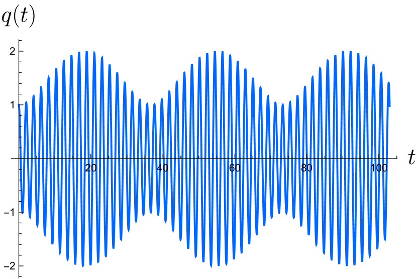
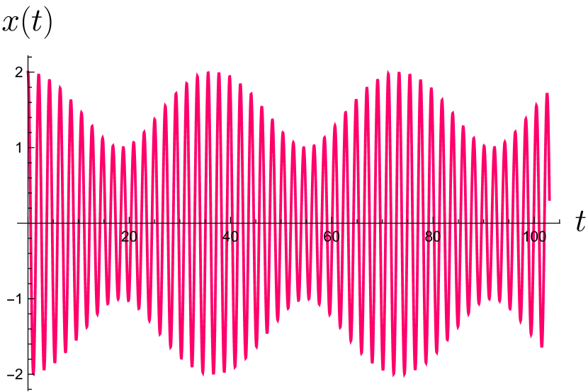
Figure 1: Evolution of the positions $q$ and $x$ of each oscillator in the weak-coupling regime for $\omega_{1}=3$, $\omega_{2}=2\sqrt{2}$ ($\omega=\sqrt{17/2}$ and $\gamma=1/2$), and initial conditions $q_{0}=1$, $x_{0}=2$, and $p_{0}=k_{0}=0$.

The equations of motion for the moments can be obtained by computing the Poisson bracket with the effective Hamiltonian (30), namely,

$$\begin{split}\frac{d}{dt}\Delta\big{(}q^{m_{1}}p^{n_{1}}x^{m_{2}}k^{n_{2}}\big{)}&=m_{1}\Delta\big{(}q^{m_{1}-1}p^{n_{1}+1}x^{m_{2}}k^{n_{2}}\big{)}-\omega^{2}n_{1}\Delta\big{(}q^{m_{1}+1}p^{n_{1}-1}x^{m_{2}}k^{n_{2}}\big{)}+m_{2}\Delta\big{(}q^{m_{1}}p^{n_{1}}x^{m_{2}-1}k^{n_{2}+1}\big{)}\\ &-\omega^{2}n_{2}\Delta\big{(}q^{m_{1}}p^{n_{1}}x^{m_{2}+1}k^{n_{2}-1}\big{)}-\gamma n_{1}\Delta\big{(}q^{m_{1}}p^{n_{1}-1}x^{m_{2}+1}k^{n_{2}}\big{)}-\gamma n_{2}\Delta\big{(}q^{m_{1}+1}p^{n_{1}}x^{m_{2}}k^{n_{2}-1}\big{)}.\end{split}$$ (39)

As commented in the previous section for quadratic Hamiltonians, these equations are linear and only couple moments of the same order. Moreover, it turns out that it is possible to write the solution of the full system in the following compact form:

$$\Delta\big{(}q^{m_{1}}p^{n_{1}}x^{m_{2}}k^{n_{2}}\big{)}= \sum_{j_{1}+j_{2}+j_{3}+j_{4}={S}}^{S}\,\frac{C_{j_{1}j_{2}j_{3}j_{4}}}{j_{1}!j_{2}!j_{3}!j_{4}!}\dfrac{\partial^{S}(q^{m_{1}}p^{n_{1}}x^{m_{2}}k^{n_{2}})}{\partial q_{0}^{j_{1}}\partial p_{0}^{j_{2}}\partial x_{0}^{j_{3}}\partial k_{0}^{j_{4}}},$$ (40)

where $S=m_{1}+n_{1}+m_{2}+n_{2}$ is the order of the moment under consideration and $C_{j_{1}j_{2}j_{3}j_{4}}:=\Delta(\tilde{q}^{j_{1}}\tilde{p}^{j_{2}}\hat{x}^{j_{3}}\hat{k}^{j_{4}})|_{t=0}$ encode the initial data at $t=0$. Note also that, in the argument of the derivative $q^{m_{1}}p^{n_{1}}x^{m_{2}}k^{n_{2}}$, one should replace the corresponding solution (35)–(38). In this way, since the evolution of the moments is expressed as a sum of partial derivatives of the expectation values $q$, $x$, $p$ and $k$, these are also periodic when $\omega_{1}$ and $\omega_{2}$ are commensurable.

As mentioned above, since the Hamiltonian is quadratic, the equations of motion for the different variables are unaffected by the nature of the different degrees of freedom, that is, it makes no difference whether they are quantum or classical. Nevertheless, the range of possible values for the initial moments $C_{m_{1}n_{1}m_{2}n_{2}}$ varies in each scenario due to the requirement imposed by the Heisenberg uncertainty principle on the quantum variables. In the case with two classical oscillators, there is not such restriction and all the moments can be vanishing, but with two quantum oscillators or in the hybrid scenario, Heisenberg uncertainty relation does not allow for an exact vanishing of all moments.

Therefore, this hybrid system can exhibit unique properties not present in classical-classical or quantum-quantum coupled oscillators. For instance, even if we choose initially vanishing fluctuations for the classical variables, $C_{m_{1}n_{1}m_{2}n_{2}}=0$ for all cases with $m_{1}+n_{1}\neq 0$, classical moments are later activated due to quantum fluctuations. The dynamics for such scenario is described by simply imposing the commented initial data in the above expression,

$$\Delta\big{(}q^{m_{1}}p^{n_{1}}x^{m_{2}}k^{n_{2}}\big{)}= \sum_{j_{1}+j_{2}={S}}^{S}\,\frac{C_{00j_{1}j_{2}}}{j_{1}!j_{2}!}\dfrac{\partial^{S}(q^{m_{1}}p^{n_{1}}x^{m_{2}}k^{n_{2}})}{\partial x_{0}^{j_{1}}\partial k_{0}^{j_{2}}},$$ (41)

From here it is possible to check that none of the moments are exactly vanishing for $t>0$, and even pure classical moments $\Delta(q^{m_{1}}p^{n_{1}})$ are activated. In order to see this fact more clearly, let us, for instance, write explicitly the evolution of the second-order moments for the classical sector:

$$\Delta(q^{2}) =\frac{1}{4}\left[\cos\left(\omega_{1}t\right)-\cos\left(\omega_{2}t\right)\right]^{2}C_{0020}+\frac{1}{4}\left[\frac{\sin\left(\omega_{1}t\right)}{\omega_{1}}-\frac{\sin\left(\omega_{2}t\right)}{\omega_{2}}\right]^{2}C_{0002}$$

$$+\frac{1}{2}\left[\cos\left(\omega_{1}t\right)-\cos\left(\omega_{2}t\right)\right]\left[\frac{\sin\left(\omega_{1}t\right)}{\omega_{1}}-\frac{\sin\left(\omega_{2}t\right)}{\omega_{2}}\right]C_{0011},$$ (42)

$$\Delta(p^{2}) =\frac{1}{4}\left[\omega_{2}\sin\left(\omega_{2}t\right)-\omega_{1}\sin\left(\omega_{1}t\right)\right]^{2}C_{0020}+\frac{1}{4}\left[\cos\left(\omega_{1}t\right)-\cos\left(\omega_{2}t\right)\right]^{2}C_{0002}$$

$$+\frac{1}{2}\left[\cos\left(\omega_{1}t\right)-\cos\left(\omega_{2}t\right)\right]\left[\omega_{2}\sin\left(\omega_{2}t\right)-\omega_{1}\sin\left(\omega_{1}t\right)\right]C_{0011},$$ (43)

$$\Delta(qp) =\frac{1}{4}\left[\omega_{2}\sin\left(\omega_{2}t\right)-\omega_{1}\sin\left(\omega_{1}t\right)\right]\left[\cos\left(\omega_{1}t\right)-\cos\left(\omega_{2}t\right)\right]C_{0020}$$

$$+\frac{1}{4}\left[\cos\left(\omega_{1}t\right)-\cos\left(\omega_{2}t\right)\right]\left[\frac{\sin\left(\omega_{1}t\right)}{\omega_{1}}-\frac{\sin\left(\omega_{2}t\right)}{\omega_{2}}\right]C_{0002}$$ (44)

$$+\frac{1}{4}\left[\cos\left(2\omega_{1}t\right)+\cos\left(2\omega_{2}t\right)-2\cos\left(\omega_{1}t\right)\cos\left(\omega_{2}t\right)+\frac{(\omega_{1}^{2}+\omega_{2}^{2})}{\omega_{1}\omega_{2}}\sin\left(\omega_{1}t\right)\sin\left(\omega_{2}t\right)\right]C_{0011}.$$

From these expressions it is clear that they are all initially vanishing but activate for $t>0$. For illustrational purposes, their evolution is also shown in Fig. 2.

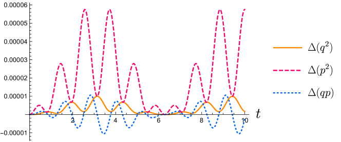
Figure 2: Evolution of the second-order moments of the classical sectors when they are initially vanishing, for $\omega_{1}=3$, $\omega_{2}=2$ ($\omega=\sqrt{13/2}$ and $\gamma=5/2$), $C_{1100}=0$, $C_{2000}=10^{-5}$ and $C_{0200}=10^{-5}$.

Moreover, another important property relies on the exchange of quantumness and classicality between different sectors. In order to analyze how the expression of the Heisenberg uncertainty relation evolves, we define the uncertainty corresponding to each degree of freedom as follows,

$$U_{q}:= \Delta(x^{2})\Delta(k^{2})-\Delta(xk)^{2},$$ (45)

$$U_{c}:= \Delta(q^{2})\Delta(p^{2})-\Delta(qp)^{2}.$$ (46)

For a purely quantum system $U_{q}\geq\hbar^{2}/4$ would be obeyed all along evolution, while for a purely classical system one would simply observe $U_{c}\geq 0$. However, in this hybrid case, considering again, for simplicity, that all the moments of the classical sector are initially vanishing, from (40), one gets

$$U_{c}=\frac{U_{0}}{16\omega_{1}^{2}\omega_{2}^{2}}\left(2\omega_{1}\omega_{2}-g(t)\right)^{2},$$ (47)

$$U_{q}=\frac{U_{0}}{16\omega_{1}^{2}\omega_{2}^{2}}\left(2\omega_{1}\omega_{2}+g(t)\right)^{2},$$ (48)

with $U_{0}:=C_{0020}C_{0002}-C_{0011}^{2}\geq\hbar^{2}/4$ being the initial uncertainty of the quantum sector, and $g$ a function defined as

$$g(t):=2\omega_{1}\omega_{2}\cos(\omega_{1}t)\cos(\omega_{2}t)+\left(\omega_{1}^{2}+\omega_{2}^{2}\right)\sin(\omega_{1}t)\sin(\omega_{2}t).$$ (49)

Therefore, dynamical properties of $U_{c}$ and $U_{q}$ rely on those of $g(t)$: both $U_{c}$ and $U_{q}$ oscillate, and, if $g(t)$ is periodic, they are also periodic, which, once again, corresponds to the case with $\omega_{2}/\omega_{1}\in\mathbb{Q}$. In addition, the upper bounds of the uncertainties are finite and are determined by the singular points of $g(t)$,

$$\begin{split}&U_{c}\leq\frac{U_{0}}{16\omega_{1}^{2}\omega_{2}^{2}}\left(2\omega_{1}\omega_{2}-g_{\min}\right)^{2}=:U_{c}^{\max},\\ &U_{q}\leq\frac{U_{0}}{16\omega_{1}^{2}\omega_{2}^{2}}\left(2\omega_{1}\omega_{2}+g_{\max}\right)^{2}=:U_{q}^{\max},\end{split}$$ (50)

where $g_{\min}$ and $g_{\max}$ correspond to the minimum and maximum values of $g(t)$, respectively. Unfortunately, it is not possible to obtain a general expression for these values for arbitrary $\omega_{1}$ and $\omega_{2}$. However, it is possible to see that they are bounded as follows,

$$\begin{split}&g_{\min}\in\left[-\left(\omega_{1}^{2}+\omega_{2}^{2}\right),-2\omega_{1}\omega_{2}\right],\\ &g_{\max}\in\left[2\omega_{1}\omega_{2},\omega_{1}^{2}+\omega_{2}^{2}\right],\end{split}$$ (51)

which provides an interval for the maximum value of the uncertainties,

$$U_{c}^{\max},U_{q}^{\max}\in\left[U_{0},\frac{\left(\omega_{1}+\omega_{2}\right)^{4}}{16\omega_{1}^{2}\omega_{2}^{2}}U_{0}\right].$$ (52)

Moreover, from (51) we deduce that the interval $[-2\omega_{1}\omega_{2},2\omega_{1}\omega_{2}]$ is in the image of $g$, and, consequently, according to (47) and (48), the uncertainties must vanish at some point. That is, their lower-bound is zero,

$$0\leq U_{c}\leq U_{c}^{\max},$$ (53)

$$0\leq U_{q}\leq U_{q}^{\max},$$ (54)

and thus the quantum sector violates, in this way, the Heisenberg uncertainty relation. In fact, from (47)–(48) one can see that the sum between the uncertainties reads,

$$U_{c}+U_{q}=\frac{U_{0}}{2}\left(1+\frac{g^{2}}{4\omega_{1}^{2}\omega_{2}^{2}}\right),$$ (55)

which has a minimum bound at $U_{0}/2$ and thus it obeys

$$U_{c}+U_{q}\geq U_{0}/2.$$ (56)

This inequality can be interpreted as the uncertainty relation of the full hybrid system: even if the Heisenberg relation of the quantum sector $U_{q}\geq\hbar^{2}/4$ is allowed to be violated by its coupling to the classical oscillator, the sum between the uncertainties $U_{c}+U_{q}$ has a minimum positive bound, which still encodes certain limit in the precision on the simultaneous knowledge of different physical properties of the system. It is interesting to note that if, instead of this hybrid system, one considered two couple quantum oscillators initially saturating both the uncertainty relation, i.e., $U_{0}=\hbar^{2}/4$ for each one, during evolution their combined uncertainty would have a minimum of $2U_{0}$, while the hybrid system presents a minimum of $U_{0}/2$. Therefore, we can state that the classical sector has two diminishing effects on the total uncertainty of the system: it does not contribute to it (since initially we can take $U_{c}=0$), but, in addition, it allows the quantum sector to decrease its own, which leads to a one fourth reduction as compared to the quantum-quantum system.

Finally, from (47)–(48) one can also obtain the following interesting relation

$$(U_{q}-U_{c}-U_{0})^{2}-4\,U_{0}\,U_{c}=0,$$ (57)

which is obeyed all along evolution. We interpret this as the conservation of the total quantumness (or classicality) of the full system. In particular, from here it is straightforward to see that, when the uncertainty of one of the sectors ($U_{c}$ or $U_{q}$) vanishes, the uncertainty of the other sector takes the value $U_{0}$, though this is not necessarily its maximum. The evolution of the uncertainty of each sector, $U_{q}$ and $U_{c}$, and of their sum $U_{c}+U_{q}$ is depicted in Fig. 3 for certain particular values of the parameters and initial conditions.

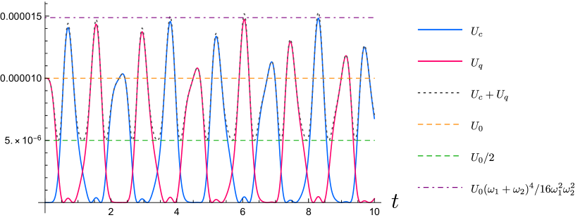
Figure 3: Evolution of the classical $U_{c}$ (in blue) and quantum $U_{q}$ (in pink) uncertainties, together with their sum $U_{c}+U_{q}$ (in gray and dotted), for $\omega_{1}=2\sqrt{2}$, $\omega_{2}=7$ ($\omega=\sqrt{57/2}$ and $\gamma=41/2$), and initial $U_{0}=10^{-5}$. The dashed orange line corresponds to the initial value $U_{0}$, the green line to the minimum value of $U_{c}+U_{q}$, given by $U_{0}/2$, and the purple one to the greatest possible upper bound for the uncertainties $U_{0}(\omega_{1}+\omega_{2})^{4}/16\omega_{1}^{2}\omega_{2}^{2}$.

7 Conclusions

We have presented a complete and consistent formalism to describe the dynamics of quantum systems, classical ensembles and, in general, hybrid systems with mixed classical and quantum sectors, for an arbitrary number of degrees of freedom. This framework is based on the decomposition of the probability distribution function of the system into its infinite set of moments. For quantum systems this formalism was already presented in Ref. [42], though here we have derived the closed formula (10) for the Poisson bracket between any two quantum moments, which corrects the expression given in that reference. (The correct expression for the case with one degree of freedom was already presented in Ref. [45].)

In addition, generalizing the work of Refs. [43, 44] to any number of degrees of freedom, we have shown that in this setup the dynamics of a classical ensemble can be described in a very similar way as that of a quantum system. In fact, the Poisson bracket between classical moments (19) takes the same form as its quantum version with $\hbar=0$. This restriction essentially drops all the purely quantum terms that come from the noncommutativity of the basic operators. In this sense, the dynamics of a classical ensemble can thus be understood as given by a truncated version of the quantum equations of motion.

In the hybrid case observables are given by products between Hermitian operators on the Hilbert space and real functions on the phase space. For such systems, starting from first principles, we have defined the hybrid bracket between observables (26), which generalizes the quantum commutator and the classical Poisson bracket. It turns out that this hybrid bracket obeys all the properties (bilinearity and antisymmetry) of a Lie bracket, except the Jacobi identity, and therefore it defines an almost Lie algebra. Then, making use of such bracket between observables, one can define a bracket for the expectation values of hybrid observables that, for the moments, takes the explicit form (23). As one would expect, this bracket does not follow the Jacobi identity either, and, along with the usual product, it provides an almost Poisson algebra. Remarkably, this bracket between hybrid moments can be derived from the bracket between quantum moments (10) simply by neglecting the $\hbar$ terms that would be present if a given classical degree of freedom was quantum.

In summary, this framework can be used to study the evolution of any hybrid system described in terms of conjugate variables and a Hamiltonian. As compared to other approaches, one of the advantages is that, unlike the probability distribution, the moments, being expectation values of observables, are physical quantities accessible by experiments. Furthermore, in this setup, it is not necessary to explicitly construct the mathematical structures on the Hilbert space and the phase space (or any other space one considers to describe the dynamics of the hybrid system), since one directly works with expectation values.

As an application of the formalism, in the last section we have studied in detail a particular hybrid system given by two (a quantum and a classical) harmonic oscillators. These oscillators are coupled by a quadratic interaction term, which allows for classical and quantum properties to be transferred between them. In particular, we have shown that the quantum oscillator is allowed to violate the Heisenberg uncertainty relation, as long as the uncertainty in the classical oscillator is not vanishing. In fact, as suggested in Ref. [15], one can define a combined uncertainty of the oscillators, which has a minimum positive bound. We have obtained this bound explicitly for the present model, and one can interpret the inequality (56) as the uncertainty relation of the full hybrid system. Interestingly, this analysis shows that the coupling of the quantum oscillator to the classical system has two diminishing effects in the total uncertainty of the system. On the one hand, the classical sector does not contribute to the total uncertainty. But, on the other hand, it also allows the quantum sector to decrease its own uncertainty. This leads to a reduction of a fourth on the total uncertainty of the hybrid system, as compared to the system given by two quantum oscillators with an initial minimum uncertainty. Finally, we have also obtained the relation (57) that can be understood as the conservation law of the total quantumness or classicality of the system.

Appendix A General properties of the Poisson bracket between expectation values

In this appendix, we will prove general properties of the Poisson bracket between expectation values. More precisely, in Sec. A.1 we will show that the Poisson bracket between the expectation value of the basic operators and any moment is vanishing. In Sec. A.2 we will derive the general formula (10) for the Poisson bracket between moments.

A.1 Poisson bracket between expectation values of the basic operators and moments

Here our goal is to show that the bracket $\{q_{i},\Delta(q_{1}^{a_{1}}p_{1}^{b_{1}}\dots q_{N}^{a_{N}}p_{N}^{b_{N}})\}$ and $\{p_{i},\Delta(q_{1}^{a_{1}}p_{1}^{b_{1}}\dots q_{N}^{a_{N}}p_{N}^{b_{N}})\}$ are vanishing. We will present the explicit computations for the former, since for the latter the derivation is equivalent.

First, we expand the expression of the moment by making use of Newton’s binomial formula, and use the linearity in the Poisson bracket to write,

$$\begin{split}\big{\{}q_{i},\Delta\big{(}q_{1}^{a_{1}}p_{1}^{b_{1}}\dots q_{N}^{a_{N}}p_{N}^{b_{N}}\big{)}\big{\}}=&\sum_{k_{1}=0}^{a_{1}}\sum_{l_{1}=0}^{b_{1}}\dots\sum_{k_{N}=0}^{a_{N}}\sum_{l_{N}=0}^{b_{N}}\left(\prod_{j=1}^{N}\binom{a_{j}}{k_{j}}\binom{b_{j}}{l_{j}}(-1)^{k_{j}+l_{j}}\right)\\ &\times\big{\{}q_{i},q_{1}^{k_{1}}p_{1}^{l_{1}}\dots q_{N}^{k_{N}}p_{N}^{l_{N}}\langle\hat{q}_{1}^{a_{1}-k_{1}}\hat{p}_{1}^{b_{1}-l_{1}}\dots\hat{q}_{N}^{a_{N}-k_{N}}\hat{p}_{N}^{b_{N}-l_{N}}\rangle_{\text{Weyl}}\big{\}}.\end{split}$$ (58)

Then, by applying the Leibniz rule and taking into account that $\{q_{i},q_{j}\}=0$ and $\{q_{i},p_{j}\}=\delta_{ij}$,

$$\begin{split}&\big{\{}q_{i},q_{1}^{k_{1}}p_{1}^{l_{1}}\dots q_{N}^{k_{N}}p_{N}^{l_{N}}\langle\hat{q}_{1}^{a_{1}-k_{1}}\hat{p}_{1}^{b_{1}-l_{1}}\dots\hat{q}_{N}^{a_{N}-k_{N}}\hat{p}_{N}^{b_{N}-l_{N}}\rangle_{\text{Weyl}}\big{\}}\\ &\,=l_{i}q_{i}^{k_{i}}p_{i}^{l_{i}-1}\langle\hat{q}_{1}^{a_{1}-k_{1}}\hat{p}_{1}^{b_{1}-l_{1}}\dots\hat{q}_{N}^{a_{N}-k_{N}}\hat{p}_{N}^{b_{N}-l_{N}}\rangle_{\text{Weyl}}\prod_{\begin{subarray}{c}j=1\\ j\neq i\end{subarray}}^{N}q_{j}^{k_{j}}p_{j}^{l_{j}}+\big{\{}q_{i},\langle\hat{q}_{1}^{a_{1}-k_{1}}\hat{p}_{1}^{b_{1}-l_{1}}\dots\hat{q}_{N}^{a_{N}-k_{N}}\hat{p}_{N}^{b_{N}-l_{N}}\rangle_{\text{Weyl}}\big{\}}\prod_{j=1}^{N}q_{j}^{k_{j}}p_{j}^{l_{j}}.\end{split}$$ (59)

Using now the definition of the Poisson bracket between expectation values, $\{\langle\hat{f}\rangle,\langle\hat{g}\rangle\}:=-i\hbar^{-1}\langle[\hat{f},\hat{g}]\rangle$, and considering that different degrees of freedom commute,

$$\begin{split}\big{\{}q_{i},\langle\hat{q}_{1}^{a_{1}-k_{1}}\hat{p}_{1}^{b_{1}-l_{1}}\dots\hat{q}_{N}^{a_{N}-k_{N}}\hat{p}_{N}^{b_{N}-l_{N}}\rangle_{\text{Weyl}}\big{\}}:=&\frac{1}{i\hbar}\bigg{\langle}\left[\hat{q}_{i},\big{(}\hat{q}_{1}^{a_{1}-k_{1}}\hat{p}_{1}^{b_{1}-l_{1}}\dots\hat{q}_{N}^{a_{N}-k_{N}}\hat{p}_{N}^{b_{N}-l_{N}}\big{)}_{\text{Weyl}}\right]\bigg{\rangle}\\ =&\frac{1}{i\hbar}\bigg{\langle}\prod_{\begin{subarray}{c}j=1\\ j\neq i\end{subarray}}^{N}\big{(}\hat{q}_{j}^{a_{j}-k_{j}}\hat{p}_{j}^{b_{j}-l_{j}}\big{)}_{\text{Weyl}}\left[\hat{q}_{i},\big{(}\hat{q}_{i}^{a_{i}-k_{i}}\hat{p}_{i}^{b_{i}-l_{i}}\big{)}_{\text{Weyl}}\right]\bigg{\rangle}\\ =&(b_{i}-l_{i})\langle\hat{q}_{1}^{a_{1}-k_{1}}\hat{p}_{1}^{b_{1}-l_{1}}\dots\hat{q}_{i}^{a_{i}-k_{i}}\hat{p}_{i}^{b_{i}-l_{i}-1}\dots\hat{q}_{N}^{a_{N}-k_{N}}\hat{p}_{N}^{b_{N}-l_{N}}\rangle_{\text{Weyl}},\end{split}$$ (60)

where we have taken into account that

$$\left[\hat{q}_{i},\big{(}\hat{q}_{i}^{a_{i}-k_{i}}\hat{p}_{i}^{b_{i}-l_{i}}\big{)}_{\text{Weyl}}\right]=i\hbar(b_{i}-l_{i})\big{(}\hat{q}_{i}^{a_{i}-k_{i}}\hat{p}_{i}^{b_{i}-l_{i}-1}\big{)}_{\text{Weyl}}.$$

Then, combining the results (58)–(60), the bracket is given as

$$\begin{split}\big{\{}q_{i},\Delta\big{(}q_{1}^{a_{1}}p_{1}^{b_{1}}\dots q_{N}^{a_{N}}p_{N}^{b_{N}}\big{)}\big{\}}&=\sum_{k_{1}=0}^{a_{1}}\sum_{l_{1}=0}^{b_{1}}\dots\sum_{k_{N}=0}^{a_{N}}\sum_{l_{N}=0}^{b_{N}}\left(\prod_{j=1}^{N}\binom{a_{j}}{k_{j}}\binom{b_{j}}{l_{j}}(-1)^{k_{j}+l_{j}}\right)\\ &\quad\times l_{i}q_{1}^{k_{1}}p_{1}^{l_{1}}\dots q_{i}^{k_{i}}p_{i}^{l_{i}-1}\dots q_{N}^{k_{N}}p_{1}^{l_{N}}\langle\hat{q}_{1}^{a_{1}-k_{1}}\hat{p}_{1}^{b_{1}-l_{1}}\dots\hat{q}_{N}^{a_{N}-k_{N}}\hat{p}_{N}^{b_{N}-l_{N}}\rangle_{\text{Weyl}}\\ &+\sum_{k_{1}=0}^{a_{1}}\sum_{l_{1}=0}^{b_{1}}\dots\sum_{k_{N}=0}^{a_{N}}\sum_{l_{N}=0}^{b_{N}}\left(\prod_{j=1}^{N}\binom{a_{j}}{k_{j}}\binom{b_{j}}{l_{j}}(-1)^{k_{j}+l_{j}}\right)\\ &\quad\times(b_{i}-l_{i})q_{1}^{k_{1}}p_{1}^{l_{1}}\dots q_{N}^{k_{N}}p_{N}^{l_{N}}\langle\hat{q}_{1}^{a_{1}-k_{1}}\hat{p}_{1}^{b_{1}-l_{1}}\dots\hat{q}_{i}^{a_{i}-k_{i}}\hat{p}_{i}^{b_{i}-l_{i}-1}\dots\hat{q}_{N}^{a_{N}-k_{N}}\hat{p}_{N}^{b_{N}-l_{N}}\rangle_{\text{Weyl}}.\end{split}$$

Finally, simplifying the binomial coefficients and performing a change of variables $l_{i}^{\prime}=l_{i}-1$ in the first term, it is straightforward to obtain

$$\begin{split}\big{\{}q_{i},\Delta\big{(}q_{1}^{a_{1}}p_{1}^{b_{1}}\dots q_{N}^{a_{N}}p_{N}^{b_{N}}\big{)}\big{\}}=0.\end{split}$$ (61)

Same rationale can be applied to prove that

$$\begin{split}\big{\{}p_{i},\Delta\big{(}q_{1}^{a_{1}}p_{1}^{b_{1}}\dots q_{N}^{a_{N}}p_{N}^{b_{N}}\big{)}\big{\}}=0.\end{split}$$ (62)

A.2 Appendix: Poisson bracket between moments

In this appendix, we will explain the key steps and properties to obtain the general formula (10) for the Poisson bracket between two arbitrary moments $\{\Delta(q_{1}^{a_{1}}p_{1}^{b_{1}}\dots q_{N}^{a_{N}}p_{N}^{b_{N}}),\Delta(q_{1}^{m_{1}}p_{1}^{n_{1}}\dots q_{N}^{m_{N}}p_{N}^{n_{N}})\}.$

Let us first present some relations that will be useful along the computation. On the one hand, from relation (60), and following the same reasoning, it is possible to obtain,

$$\begin{split}\big{\{}p_{i},\langle\hat{q}_{1}^{a_{1}-k_{1}}\hat{p}_{1}^{b_{1}-l_{1}}\dots\hat{q}_{N}^{a_{N}-k_{N}}\hat{p}_{N}^{b_{N}-l_{N}}\rangle_{\text{Weyl}}\big{\}}=&-(a_{i}-k_{i})\langle\hat{q}_{1}^{a_{1}-k_{1}}\hat{p}_{1}^{b_{1}-l_{1}}\dots\hat{q}_{i}^{a_{i}-k_{i}-1}\hat{p}_{i}^{b_{i}-l_{i}}\dots\hat{q}_{N}^{a_{N}-k_{N}}\hat{p}_{N}^{b_{N}-l_{N}}\rangle_{\text{Weyl}}.\end{split}$$ (63)

On the other hand, making use of the following properties for reordering quantum operators,

$$\big{(}\hat{q}_{j}^{m}\hat{p}_{j}^{n}\big{)}_{\text{Weyl}} =\sum_{k=0}^{\min({m,n})}\left(\frac{i\hbar}{2}\right)^{k}k!\binom{n}{k}\binom{m}{k}\hat{p}_{j}^{n-k}\hat{q}_{j}^{m-k}$$ (64)

$$=\sum_{k=0}^{\min({m,n})}(-1)^{k}\left(\frac{i\hbar}{2}\right)^{k}k!\binom{n}{k}\binom{m}{k}\hat{q}_{j}^{m-k}\hat{p}_{j}^{n-k},$$ (65)

$$\hat{p}_{j}^{n}\hat{q}_{j}^{m}=\sum_{k=0}^{\min({m,n})}(-1)^{k}\left(\frac{i\hbar}{2}\right)^{k}k!\binom{n}{k}\binom{m}{k}\big{(}\hat{q}_{j}^{m-k}\hat{p}_{j}^{n-k}\big{)}_{\text{Weyl}},$$ (66)

$$\hat{q}_{j}^{m}\hat{p}_{j}^{n}=\sum_{k=0}^{\min({m,n})}\left(\frac{i\hbar}{2}\right)^{k}k!\binom{n}{k}\binom{m}{k}\big{(}\hat{q}_{j}^{m-k}\hat{p}_{j}^{n-k}\big{)}_{\text{Weyl}},$$ (67)

$$\big{[}\hat{q}_{j}^{m},\hat{p}_{j}^{n}\big{]}=\sum_{k=1}^{\min({m,n})}\left(i\hbar\right)^{k}k!\binom{n}{k}\binom{m}{k}\hat{p}_{j}^{n-k}\hat{q}_{j}^{m-k}=-\sum_{k=1}^{\min({m,n})}(-1)^{k}\left(i\hbar\right)^{k}k!\binom{n}{k}\binom{m}{k}\hat{q}_{j}^{m-k}\hat{p}_{j}^{n-k},$$ (68)

it is possible to obtain the key relations,

$$\big{(}\hat{q}_{j}^{m}\hat{p}_{j}^{n}\big{)}_{\text{Weyl}}\big{(}\hat{q}_{j}^{s}\hat{p}_{j}^{r}\big{)}_{\text{Weyl}} =\sum_{\alpha=0}^{M^{\prime}}\bigg{(}\frac{i\hbar}{2}\bigg{)}^{\alpha}K^{\alpha}_{mnsr}\big{(}\hat{q}_{j}^{m+s-\alpha}\hat{p}_{j}^{n+r-\alpha}\big{)}_{\text{Weyl}},$$ (69)

$$\left[\big{(}\hat{q}_{j}^{m}\hat{p}_{j}^{n}\big{)}_{\text{Weyl}},\big{(}\hat{q}_{j}^{s}\hat{p}_{j}^{r}\big{)}_{\text{Weyl}}\right] =\sum_{\text{odd\;}\alpha=1}^{M^{\prime}}2\bigg{(}\frac{i\hbar}{2}\bigg{)}^{\alpha}K^{\alpha}_{mnsr}\big{(}\hat{q}_{j}^{m+s-\alpha}\hat{p}_{j}^{n+r-\alpha}\big{)}_{\text{Weyl}},$$ (70)

with $M^{\prime}:=\min(m+s,m+n,n+r,s+r)$ and

$$K_{abmn}^{\alpha}:=\sum_{k=0}^{\alpha}(-1)^{k}k!(\alpha-k)!\binom{a}{\alpha-k}\binom{b}{k}\binom{m}{k}\binom{n}{\alpha-k}.$$ (71)

Now we are in a position to compute the bracket $\{\Delta(q_{1}^{a_{1}}p_{1}^{b_{1}}\dots q_{N}^{a_{N}}p_{N}^{b_{N}}),\Delta(q_{1}^{m_{1}}p_{1}^{n_{1}}\dots q_{N}^{m_{N}}p_{N}^{n_{N}})\}.$ First, we expand one of the moments by applying Newton’s binomial formula, and using linearity of the Poisson bracket, we write

$$\begin{split}&\left\{\Delta\big{(}q_{1}^{a_{1}}p_{1}^{b_{1}}\dots q_{N}^{a_{N}}p_{N}^{b_{N}}\big{)},\Delta\big{(}q_{1}^{m_{1}}p_{1}^{n_{1}}\dots q_{N}^{m_{N}}p_{N}^{n_{N}}\big{)}\right\}\\ &\;=\sum_{r_{1}=0}^{m_{1}}\sum_{s_{1}=0}^{n_{1}}\dots\sum_{r_{N}=0}^{m_{N}}\sum_{s_{N}=0}^{n_{N}}\left(\prod_{j=1}^{N}\binom{m_{j}}{r_{j}}\binom{n_{j}}{s_{j}}(-1)^{r_{j}+s_{j}}\right)\\ &\;\,\quad\times\big{\{}\Delta\big{(}q_{1}^{a_{1}}p_{1}^{b_{1}}\dots q_{N}^{a_{N}}p_{N}^{b_{N}}\big{)},q_{1}^{r_{1}}p_{1}^{s_{1}}\dots q_{N}^{r_{N}}p_{N}^{s_{N}}\langle\hat{q}_{1}^{m_{1}-r_{1}}\hat{p}_{1}^{n_{1}-s_{1}}\dots\hat{q}_{N}^{m_{N}-r_{N}}\hat{p}_{N}^{n_{N}-s_{N}}\rangle_{\text{Weyl}}\big{\}}.\end{split}$$ (72)

Then, by applying the Leibniz rule and taking into account that expectation values $q_{i}$ and $p_{i}$ have a vanishing Poisson bracket with any moment (relations (61) and (62)),

$$\begin{split}\left\{\Delta\big{(}q_{1}^{a_{1}}p_{1}^{b_{1}}\dots q_{N}^{a_{N}}p_{N}^{b_{N}}\big{)},\Delta\big{(}q_{1}^{m_{1}}p_{1}^{n_{1}}\dots q_{N}^{m_{N}}p_{N}^{n_{N}}\big{)}\right\}=&\sum_{r_{1}=0}^{m_{1}}\sum_{s_{1}=0}^{n_{1}}\dots\sum_{r_{N}=0}^{m_{N}}\sum_{s_{N}=0}^{n_{N}}\left(\prod_{j=1}^{N}\binom{m_{j}}{r_{j}}\binom{n_{j}}{s_{j}}(-1)^{r_{j}+s_{j}}q_{j}^{r_{j}}p_{j}^{s_{j}}\right)\\ &\times\big{\{}\Delta\big{(}q_{1}^{a_{1}}p_{1}^{b_{1}}\dots q_{N}^{a_{N}}p_{N}^{b_{N}}\big{)},\langle\hat{q}_{1}^{m_{1}-r_{1}}\hat{p}_{1}^{n_{1}-s_{1}}\dots\hat{q}_{N}^{m_{N}-r_{N}}\hat{p}_{N}^{n_{N}-s_{N}}\rangle_{\text{Weyl}}\big{\}}.\end{split}$$ (73)

Now, we expand the other moment by using Newton’s binomial formula, and considering the linearity of the bracket, we get

$$\begin{split}&\big{\{}\Delta\big{(}q_{1}^{a_{1}}p_{1}^{b_{1}}\dots q_{N}^{a_{N}}p_{N}^{b_{N}}\big{)},\langle\hat{q}_{1}^{m_{1}-r_{1}}\hat{p}_{1}^{n_{1}-s_{1}}\dots\hat{q}_{N}^{m_{N}-r_{N}}\hat{p}_{N}^{n_{N}-s_{N}}\rangle_{\text{Weyl}}\big{\}}\\ &\,=\sum_{k_{1}=0}^{a_{1}}\sum_{l_{1}=0}^{b_{1}}\dots\sum_{k_{N}=0}^{a_{N}}\sum_{l_{N}=0}^{b_{N}}\left(\prod_{j=1}^{N}\binom{a_{j}}{k_{j}}\binom{b_{j}}{r_{j}}(-1)^{k_{j}+r_{j}}\right)\\ &\,\quad\times\big{\{}q_{1}^{k_{1}}p_{1}^{l_{1}}\dots q_{N}^{k_{N}}p_{N}^{l_{N}}\langle\hat{q}_{1}^{a_{1}-k_{1}}\hat{p}_{1}^{b_{1}-r_{1}}\dots\hat{q}_{N}^{a_{N}-k_{N}}\hat{p}_{N}^{b_{N}-r_{N}}\rangle_{\text{Weyl}},\langle\hat{q}_{1}^{m_{1}-r_{1}}\hat{p}_{1}^{n_{1}-s_{1}}\dots\hat{q}_{N}^{m_{N}-r_{N}}\hat{p}_{N}^{n_{N}-s_{N}}\rangle_{\text{Weyl}}\big{\}}.\end{split}$$ (74)

Next, by applying the Leibniz rule, and taking into account (60) and (63),

$$\begin{split}&\big{\{}q_{1}^{k_{1}}p_{1}^{l_{1}}\dots q_{N}^{k_{N}}p_{N}^{l_{N}}\langle\hat{q}_{1}^{a_{1}-k_{1}}\hat{p}_{1}^{b_{1}-r_{1}}\dots\hat{q}_{N}^{a_{N}-k_{N}}\hat{p}_{N}^{b_{N}-r_{N}}\rangle_{\text{Weyl}},\langle\hat{q}_{1}^{m_{1}-r_{1}}\hat{p}_{1}^{n_{1}-s_{1}}\dots\hat{q}_{N}^{m_{N}-r_{N}}\hat{p}_{N}^{n_{N}-s_{N}}\rangle_{\text{Weyl}}\big{\}}\\ &\,=\sum_{j=1}^{N}\langle\hat{q}_{1}^{a_{1}-k_{1}}\hat{p}_{1}^{b_{1}-r_{1}}\dots\hat{q}_{N}^{a_{N}-k_{N}}\hat{p}_{N}^{b_{N}-r_{N}}\rangle_{\text{Weyl}}\prod_{\begin{subarray}{c}i=1\\ i\neq j\end{subarray}}^{N}q_{i}^{k_{i}}p_{i}^{l_{i}}\\ &\,\quad\times\bigg{(}k_{j}(n_{j}-s_{j})q_{j}^{k_{j}-1}p_{j}^{l_{j}}\langle\hat{q}_{1}^{m_{1}-r_{1}}\hat{p}_{1}^{n_{1}-s_{1}}\dots\hat{q}_{j}^{m_{j}-r_{j}}\hat{p}_{j}^{n_{j}-s_{j}-1}\dots\hat{q}_{N}^{m_{N}-r_{N}}\hat{p}_{N}^{n_{N}-s_{N}}\rangle_{\text{Weyl}}\\ &\,\qquad\quad-l_{j}(m_{j}-r_{j})q_{j}^{k_{j}}p_{j}^{l_{j}-1}\langle\hat{q}_{1}^{m_{1}-r_{1}}\hat{p}_{1}^{n_{1}-s_{1}}\dots\hat{q}_{j}^{m_{j}-r_{j}-1}\hat{p}_{j}^{n_{j}-s_{j}}\dots\hat{q}_{N}^{m_{N}-r_{N}}\hat{p}_{N}^{n_{N}-s_{N}}\rangle_{\text{Weyl}}\bigg{)}\\ &\,+q_{1}^{k_{1}}p_{1}^{l_{1}}\dots q_{N}^{k_{N}}p_{N}^{l_{N}}\big{\{}\langle\hat{q}_{1}^{a_{1}-k_{1}}\hat{p}_{1}^{b_{1}-r_{1}}\dots\hat{q}_{N}^{a_{N}-k_{N}}\hat{p}_{N}^{b_{N}-r_{N}}\rangle_{\text{Weyl}},\langle\hat{q}_{1}^{m_{1}-r_{1}}\hat{p}_{1}^{n_{1}-s_{1}}\dots\hat{q}_{N}^{m_{N}-r_{N}}\hat{p}_{N}^{n_{N}-s_{N}}\rangle_{\text{Weyl}}\big{\}}.\end{split}$$ (75)

Then, by applying the definition of the Poisson bracket between expectation values, $\{\langle\hat{f}\rangle,\langle\hat{g}\rangle\}:=-i\hbar^{-1}\langle[\hat{f},\hat{g}]\rangle$, taking into account that different degrees of freedom commute and the properties (69)–(70), the last line of (75) can be written as

$$\begin{split}&\big{\{}\langle\hat{q}_{1}^{a_{1}-k_{1}}\hat{p}_{1}^{b_{1}-r_{1}}\dots\hat{q}_{N}^{a_{N}-k_{N}}\hat{p}_{N}^{b_{N}-r_{N}}\rangle_{\text{Weyl}},\langle\hat{q}_{1}^{m_{1}-r_{1}}\hat{p}_{1}^{n_{1}-s_{1}}\dots\hat{q}_{N}^{m_{N}-r_{N}}\hat{p}_{N}^{n_{N}-s_{N}}\rangle_{\text{Weyl}}\big{\}}\\ &\,=\sum_{L=0}^{M^{\prime\prime}}(-1)^{L}\left(\frac{\hbar}{2}\right)^{2L}\prod_{j=1}^{N}K^{\alpha_{j}}_{a_{j}-k_{j},b_{j}-r-j,m_{j}-r_{j},n_{j}-s_{j}}\\ &\,\quad\times\langle\hat{q}_{1}^{a_{1}-k_{1}+m_{1}-r_{1}-\alpha_{1}}\hat{p}_{1}^{b_{1}-l_{1}+n_{1}-s_{1}-\alpha_{1}}\dots\hat{q}_{N}^{a_{N}-k_{N}+m_{N}-r_{N}-\alpha_{N}}\hat{p}_{N}^{b_{N}-l_{N}+n_{N}-s_{N}-\alpha_{N}}\rangle_{\text{Weyl}},\end{split}$$ (76)

where we have also considered the Leibniz rule inside the commutator. Here, we define $2L+1:=\alpha_{1}+\dots+\alpha_{N}$ and, for each value of $L$, we must consider all possible combinations of the integers $\alpha_{j}\in[0,M^{\prime}_{j}]$, with $M^{\prime}_{j}:=\min(a_{j}+m_{j}-k_{j}-r_{j},b_{j}+n_{j}-l_{j}-s_{j},a_{j}+b_{j}-k_{j}-l_{j},m_{j}+n_{j}-r_{j}-s_{j})$.

Finally, by combining (72)–(76), and doing some combinatorics with the series, one gets the result

$$\begin{split}&\left\{\Delta\big{(}q_{1}^{a_{1}}p_{1}^{b_{1}}\dots q_{N}^{a_{N}}p_{N}^{b_{N}}\big{)},\Delta\big{(}q_{1}^{m_{1}}p_{1}^{n_{1}}\dots q_{N}^{m_{N}}p_{N}^{n_{N}}\big{)}\right\}\\ &\;=\sum_{j=1}^{N}\bigg{(}b_{j}\,m_{j}\,\Delta\big{(}q_{1}^{a_{1}}p_{1}^{b_{1}}\dots q_{j}^{a_{j}}p_{j}^{b_{j}-1}\dots q_{N}^{a_{N}}p_{N}^{b_{N}}\big{)}\,\Delta(q_{1}^{m_{1}}p_{1}^{n_{1}}\dots q_{j}^{m_{j}-1}p_{j}^{n_{j}}\dots q_{N}^{m_{N}}p_{N}^{n_{N}})\\ &\;\qquad\quad\;\;-a_{j}\,n_{j}\,\Delta\big{(}q_{1}^{a_{1}}p_{1}^{b_{1}}\dots q_{j}^{a_{j}-1}p_{j}^{b_{j}}\dots q_{N}^{a_{N}}p_{N}^{b_{N}}\big{)}\,\Delta(q_{1}^{m_{1}}p_{1}^{n_{1}}\dots q_{j}^{m_{j}}p_{j}^{n_{j}-1}\dots q_{N}^{m_{N}}p_{N}^{n_{N}})\bigg{)}\\ &\;+\sum_{L=0}^{M}(-1)^{L}\left(\frac{\hbar}{2}\right)^{2L}K^{\alpha_{1}}_{a_{1}b_{1}m_{1}n_{1}}\dots K^{\alpha_{N}}_{a_{N}b_{N}m_{N}n_{N}}\Delta\big{(}q_{1}^{a_{1}+m_{1}-\alpha_{1}}p_{1}^{b_{1}+n_{1}-\alpha_{1}}\dots q_{N}^{a_{N}+m_{N}-\alpha_{N}}p_{N}^{b_{N}+n_{N}-\alpha_{N}}\big{)},\end{split}$$ (77)

where $2L+1:=\alpha_{1}+\dots+\alpha_{N}$ and, for each value of $L$, all possible combinations of the integers $\alpha_{j}\in[0,M_{j}]$ should be considered, with, $M_{j}:=\min(a_{j}+m_{j},b_{j}+n_{j},a_{j}+b_{j},m_{j}+n_{j})$. Thus, the upper bound of the sum in $L$ is thus given by $M:=(-1+\sum_{j=1}^{N}M_{j})/2$.

Appendix B The almost Lie hybrid bracket

Let us provide a systematic construction of the hybrid bracket $[\![\overline{A},\overline{B}]\!]$ between two generic hybrid observables $\overline{A},\overline{B}\in{\cal A}$ beginning from first principles. First, these being two fundamental properties of any Lie bracket, we will require it to be bilinear and antisymmetric:

$$[\![\overline{A},\overline{B}]\!] =-[\![\overline{B},\overline{A}]\!],$$ (78)

$$[\![a_{1}\overline{A}_{1}+a_{2}\overline{A}_{2},\overline{B}]\!] =a_{1}[\![\overline{A}_{1},\overline{B}]\!]+a_{2}[\![\overline{A}_{2},\overline{B}]\!],$$ (79)

for any real numbers $a_{1},a_{2}$. Then, as suggested in Ref. [47], we will also require that

$$[\![\overline{A},\overline{B}]\!]^{\dagger} =[\![\overline{A},\overline{B}]\!],$$ (80)

with ^† being the complex conjugate, which implies that an Hermitian operator (an observable) will remain so under dynamical evolution, and

$$[\![\tilde{f},\tilde{g}\hat{G}]\!]=\big{\{}\tilde{f},\tilde{g}\big{\}}_{c}\hat{G}, \qquad[\![\hat{F},\tilde{g}\hat{G}]\!]=\frac{1}{i\hbar}\left[\hat{F},\hat{G}\right]\tilde{g},$$ (81)

for $\forall\tilde{f},\tilde{g}\in\mathscr{A}_{c}$ and $\forall\hat{F},\hat{G}\in\mathscr{A}_{q}$. This last requirement, combined with the bilinearity (79), dictates several properties in a very compact way:

• The bracket must reduce to the classical Poisson bracket or the commutator (times $-i/\hbar$) when both arguments are classical or quantum observables, respectively,

  $$[\![\tilde{f},\tilde{g}]\!]=\big{\{}\tilde{f},\tilde{g}\big{\}}_{c}, \qquad[\![\hat{F},\hat{G}]\!]=\frac{1}{i\hbar}\left[\hat{F},\hat{G}\right].$$

• The bracket between a classical and a quantum operator vanishes:

  $$[\![\tilde{f},\hat{Q}]\!]=\big{\{}\tilde{f},1\big{\}}_{c}\hat{Q}=0.$$

  Hence, when the quantum and classical sectors are dynamically uncoupled, i.e., when the Hamiltonian is of the form $\overline{H}=\hat{Q}+\tilde{C}$, the different sectors evolve independently; in particular, an observable of the form $\tilde{f}\hat{G}$ will evolve to $\tilde{f}(t)\hat{G}(t)$.

• Since the identity $\mathds{1}$ is simultaneously a classical and a quantum observable:

  $$[\![\mathds{1},\tilde{g}\hat{G}]\!]=\big{\{}\mathds{1},\tilde{g}\big{\}}_{c}\hat{G}=0.$$

  Consequently, a constant operator will not evolve.

Therefore, taking the properties (78)–(81) into account, we propose the following definition:

$$\begin{split}&[\![\tilde{f}\hat{F},\tilde{g}\hat{G}]\!]:=\big{\{}\tilde{f},\tilde{g}\big{\}}_{c}R(\hat{F},\hat{G})+\frac{1}{i\hbar}\left[\hat{F},\hat{G}\right]\tilde{f}\tilde{g},\end{split}$$ (82)

where $\tilde{f},\tilde{g}\in\mathscr{A}_{c}$ and $\hat{F},\hat{G}\in\mathscr{A}_{q}$. As evident, definition (82) applies specifically to just two products; however, by imposing bilinearity to the hybrid bracket, it can be extended to encompass any pair of hybrid observables (since any of these can be expressed as a linear combination of products $\tilde{f}_{i}\hat{F}_{j}$). $R$ is a mapping $R:\mathscr{A}_{q}\times\mathscr{A}_{q}\to\mathscr{A}_{q}$ and, in what follows, we will analyze the conditions that it has to satisfy so that properties (78)–(81) are ensured. In what follows, $\hat{F},\hat{G},\hat{F}_{1},\hat{F}_{2}\in\mathscr{A}_{q}$ will denote any generic operators in ${\cal A}_{q}$, $\tilde{f},\tilde{g}\in\mathscr{A}_{c}$ any classical observables, and $a_{1},a_{2}\in\mathbb{R}$ any real numbers.

1. First, since both the commutator and the classical Poisson bracket are antisymmetric, for the hybrid bracket (82) to be antisymmetric (78), the mapping $R$ needs to be symmetric:

   $$R(\hat{F},\hat{G})=R(\hat{G},\hat{F}).$$ (83)

2. Second, since the hybrid bracket has to be linear (79) in its first argument, it must obey

   $$[\![\tilde{f}(a_{1}\hat{F}_{1}+a_{2}\hat{F}_{2}),\tilde{g}\hat{G}]\!]=a_{1}[\![\tilde{f}\hat{F}_{1},\tilde{g}\hat{G}]\!]+a_{2}[\![\tilde{f}\hat{F}_{2},\tilde{g}\hat{G}]\!].$$

   Then, by making use of definition (82) in both sides of the last equation, one gets

   $$\big{\{}\tilde{f},\tilde{g}\big{\}}_{c}R(a_{1}\hat{F}_{1}+a_{2}\hat{F}_{2},\hat{G})+a_{1}\frac{1}{i\hbar}\left[\hat{F}_{1},\hat{G}_{1}\right]\tilde{f}\tilde{g}+a_{2}\frac{1}{i\hbar}\left[\hat{F}_{2},\hat{G}_{1}\right]\tilde{f}\tilde{g}$$

   $$=a_{1}\big{\{}\tilde{f},\tilde{g}\big{\}}_{c}R(\hat{F}_{1},\hat{G})+a_{1}\frac{1}{i\hbar}\left[\hat{F}_{1},\hat{G}_{1}\right]\tilde{f}\tilde{g}+a_{2}\big{\{}\tilde{f},\tilde{g}\big{\}}_{c}R(\hat{F}_{2},\hat{G})+a_{2}\frac{1}{i\hbar}\left[\hat{F}_{2},\hat{G}_{1}\right]\tilde{f}\tilde{g},$$

   where we have used that the commutator is bilinear. Then, simplifying and grouping terms, one gets that

   $$R(a_{1}\hat{F}_{1}+a_{2}\hat{F}_{2},\hat{G})=a_{1}R(\hat{F}_{1},\hat{G})+a_{2}R(\hat{F}_{2},\hat{G}).$$ (84)

   The same reasoning can be made for linearity in the second argument of the bracket and obtain

   $$R(\hat{G},a_{1}\hat{F}_{1}+a_{2}\hat{F}_{2})=a_{1}R(\hat{G},\hat{F}_{1})+a_{2}R(\hat{G},\hat{F}_{2}).$$ (85)

   Hence, the bracket (82) will be bilinear, and thus obey (79), if $R$ is also bilinear.

3. Third, due to condition (80), $[\![\tilde{f}\hat{F},\tilde{g}\hat{G}]\!]$ has to be Hermitian, that is,

   $$[\![\tilde{f}\hat{F},\tilde{g}\hat{G}]\!]=[\![\tilde{f}\hat{F},\tilde{g}\hat{G}]\!]^{\dagger}.$$

   Using definition (82), and taking into account that $\frac{1}{i\hbar}[\hat{F},\hat{G}]$ is Hermitian, one gets that

   $$R(\hat{F},\hat{G})^{\dagger}=R(\hat{F},\hat{G}).$$ (86)

4. Fourth, since the identity $\hat{\mathds{1}}$ commutes with any operator, $[\hat{\mathds{1}},\hat{G}]=0$, and using the first equality of (81), one can write

   $$\big{\{}\tilde{f},\tilde{g}\big{\}}_{c}\hat{G}\stackrel{{\scriptstyle\eqref{properties_bracket_mix}}}{{=}}[\![\tilde{f},\tilde{g}\hat{G}]\!] :=\big{\{}\tilde{f},\tilde{g}\big{\}}_{c}R(\hat{\mathds{1}},\hat{G})+\frac{1}{i\hbar}\left[\hat{\mathds{1}},\hat{G}\right]\tilde{f}\tilde{g}=\big{\{}\tilde{f},\tilde{g}\big{\}}_{c}R(\hat{\mathds{1}},\hat{G}).$$

   Thus, condition (81) imposes that $\hat{\mathds{1}}$ must be the identity for the mapping $R$:

   $$R(\hat{\mathds{1}},\hat{G})=\hat{G}.$$ (87)

   Finally, the second equality of condition (81), $[\![\hat{F},\tilde{g}\hat{G}]\!]:=-i\hbar^{-1}[\hat{F},\hat{G}]\tilde{g}$, is directly satisfied by definition (82) since $\{\mathds{1},\tilde{g}\}=0$.

In summary, the hybrid bracket (82) will obey the basic conditions (78)–(81) if the mapping $R$ is symmetric (83), bilinear (84)–(85), Hermitian (86), and the identity operator is also its identity (87).

Let us thus now turn our attention to the last fundamental requirement for (82) to be a Lie bracket: the Jacobi identity. As explained in the text, being a hybrid bracket, it cannot obey such identity since this would produce certain inconsistencies in the dynamics (see [46]). However, since we still have some freedom to define $R$, one can use the failure to fulfill the Jacobi identity as a guidance/additional requirement. More precisely, we define the jacobiator of the hybrid bracket as,

$$\mathscr{J}:=[\![\overline{A},[\![\overline{B},\overline{C}]\!]]\!]+[\![\overline{B},[\![\overline{C},\overline{A}]\!]]\!]+[\![\overline{C},[\![\overline{A},\overline{B}]\!]]\!],$$ (88)

for certain hybrid observables $\overline{A},\overline{B},\overline{C}\in\mathscr{A}$. Now, making use of definition (82), taking bilinearity into account, and considering $\overline{A}=\tilde{a}\hat{A}$, $\overline{B}=\tilde{b}\hat{B}$ and $\overline{C}=\tilde{c}\hat{C}$, the jacobiator reads

$$\begin{split}\mathscr{J}&=R\left(\hat{A},R(\hat{B},\hat{C})\right)\big{\{}\tilde{a},\big{\{}\tilde{b},\tilde{c}\big{\}}_{c}\big{\}}_{c}+R\left(\hat{B},R(\hat{C},\hat{A})\right)\big{\{}\tilde{b},\big{\{}\tilde{c},\tilde{a}\big{\}}_{c}\big{\}}_{c}+R\left(\hat{C},R(\hat{A},\hat{B})\right)\big{\{}\tilde{c},\big{\{}\tilde{a},\tilde{b}\big{\}}_{c}\big{\}}_{c}\\ &\quad+\frac{1}{i\hbar}\tilde{a}\big{\{}\tilde{b},\tilde{c}\big{\}}_{c}\left(\big{[}\hat{A},R(\hat{B},\hat{C})\big{]}+R\big{(}\hat{B},\big{[}\hat{C},\hat{A}\big{]}\big{)}-R\big{(}\hat{C},\big{[}\hat{A},\hat{B}\big{]}\big{)}\right)\\ &\quad+\frac{1}{i\hbar}\tilde{b}\big{\{}\tilde{c},\tilde{a}\big{\}}_{c}\left(\big{[}\hat{B},R(\hat{C},\hat{A})\big{]}+R\big{(}\hat{C},\big{[}\hat{A},\hat{B}\big{]}\big{)}-R\big{(}\hat{A},\big{[}\hat{B},\hat{C}\big{]}\big{)}\right)\\ &\quad+\frac{1}{i\hbar}\tilde{c}\big{\{}\tilde{a},\tilde{b}\big{\}}_{c}\left(\big{[}\hat{C},R(\hat{A},\hat{B})\big{]}+R\big{(}\hat{A},\big{[}\hat{B},\hat{C}\big{]}\big{)}-R\big{(}\hat{B},\big{[}\hat{C},\hat{A}\big{]}\big{)}\right),\end{split}$$ (89)

where we have also taken into account that the commutator satisfies the Jacobi identity. From here one can see that there are two types of terms in $J$. The first three terms are products between operators and double classical Poisson brackets. In fact, if one requests that

$$R\left(\hat{A},R(\hat{B},\hat{C})\right)=R\left(\hat{B},R(\hat{C},\hat{A})\right)=R\left(\hat{C},R(\hat{A},\hat{B})\right),$$ (90)

and use the fact that the classical Poisson bracket obeys the Jacobi identity, these first three terms would vanish. Therefore, (90) is a natural and simple condition for $R$ that we will also require. The remaining terms in (89) are more involved since they mix the action of $R$ and the commutator, so it is not possible to obtain a simple requirement for $R$ so that they all would be vanishing. These are indeed the terms that are responsible for the jacobiator not to be vanishing in the hybrid case. Note, however, that if one computes the jacobiator for purely quantum (with $\tilde{a}=\tilde{b}=\tilde{c}=1$) or purely classical (with $\hat{A}=\hat{B}=\hat{C}=\hat{\mathds{1}}$) observables, the expression (89) would automatically vanish and the Jacobi identity would be fulfilled.

Therefore, taking all the discussion above into account, we propose the following action for the mapping $R$:

$$R\left(\big{(}\hat{q}_{1}^{m_{1}}\hat{p}_{1}^{n_{1}}\dots\hat{q}_{N}^{m_{N}}\hat{p}_{N}^{n_{N}}\big{)}_{\text{Weyl}},\big{(}\hat{q}_{1}^{k_{1}}\hat{p}_{1}^{l_{1}}\dots\hat{q}_{N}^{k_{N}}\hat{p}_{N}^{l_{N}}\big{)}_{\text{Weyl}}\right):=\big{(}\hat{q}_{1}^{m_{1}+k_{1}}\hat{p}_{1}^{n_{1}+l_{1}}\dots\hat{q}_{N}^{m_{N}+k_{N}}\hat{p}_{N}^{n_{N}+l_{N}}\big{)}_{\text{Weyl}},$$ (91)

which satisfies conditions (83)–(87) and (90). Making then use of the hybrid bracket (82) given by this definition of $R$, it is possible to show that the Poisson bracket between expectation values, defined as $\{\langle\cdot{}\rangle,\langle\cdot{}\rangle\}:=\langle[\![\cdot{},\cdot{}]\!]\rangle$, leads to the explicit form (23) for the case of two generic moments.Note that this definition of $R$ is given only for Weyl-ordered products of basic quantum operators. However, as commented in the main text, since it is bilinear, its action can be extended to any arbitrary operator by considering an expansion of the form (20).

References

• [1] N. Bohr, Atomic Physics and Human Knowledge (Wiley, New York, 1958).
• [2] W. Heisenberg, Physics and Philosophy: The Revolution in Modern Science (Harper Perennial Modern Classics, London, 2007).
• [3] B. dโ€™Espagnat, Conceptual Foundations of Quantum Mechanics (Addison Wesley, Reading, 1976).
• [4] A. E. Allahverdyan, R. Balian, and T.M. Nieuwenhuizen, Phys. Rept. 525, 1 (2013).
• [5] W. Boucher and J. Traschen, Phys. Rev. D 37, 3522 (1988).
• [6] J.ย Oppenheim, Phys. Rev. X 13, 041040 (2023).
• [7] J. ร…qvist and A. Warshel, Chem. Rev. 93, 2523 (1993).
• [8] G. Monard, M. Loos, V. Thรฉry, K. Baka, and J-L. Rivail, Int. J. Quantum Chem. 58, 153 (1996).
• [9] F. A. Bornemann, P. Nettesheim, and C. Schรผtte, J. Chem. Phys. 105, 1074 (1996).
• [10] O. V. Prezhdo and P. J. Rossky, J. Chem. Phys. 107, 825 (1997).
• [11] R. Kapral and G. Ciccotti, J. Chem. Phys. 110, 8919 (1999).
• [12] G. Csรกnyi, T. Albaret, M. C. Payne, and A. De Vita, Phys. Rev. Lett. 93, 175503 (2004).
• [13] R.ย Crespo-Otero and M.ย Barbatti, Chemical reviews 118, 7026 (2018).
• [14] D.ย R.ย Terno, arXiv:2309.05014 [quant-ph] (2023).
• [15] C.ย Barcelo, R.ย Carballo-Rubio, L.ย J.ย Garay, and R.ย Gomez-Escalante, Phys. Rev. A 86, 042120 (2012).
• [16] A. Anderson, Phys. Rev. Lett. 74, 621 (1995).
• [17] B. O. Koopman, Proceedings of the National Academy of Sciences 17, 315 (1931).
• [18] J. von Neumann, Ann. Math. 33, 587 (1932).
• [19] E. C. G. Sudarshan, Pramana 6, 117 (1976).
• [20] T. N. Sherry and E. C. G. Sudarshan, Phys. Rev. D 18, 4580 (1978).
• [21] T. N. Sherry and E. C. G. Sudarshan, Phys. Rev. D 20, 857 (1979).
• [22] S. R. Gautam, T. N. Sherry, and E. C. G. Sudarshan, Phys. Rev. D 20, 3081 (1979).
• [23] I.ย V.ย Aleksandrov, Zeitschrift fรผr Naturforschung A 36, 902โ€“908 (1981).
• [24] V.ย I.ย Gerasimenko, Theoretical and Mathematical Physics 50, 49 (1982).
• [25] P. Blanchard and A. Jadczyk, Physics Letters A 175, 157 (1993).
• [26] A.ย Peres and D.ย R.ย  Terno, Phys. Rev. A 63, 022101 (2001).
• [27] D. R. Terno, Found. Phys. 36, 102 (2006).
• [28] L.ย Diรณsi, Phys. Rev. A 107, 062206 (2023).
• [29] F.ย Gay-Balmaz and C.ย Tronci, Physica D: Nonlinear Phenomena 440, 133450 (2022).
• [30] A.ย D.ย Bermรบdez Manjarres, J. Phys. A 54, 444001 (2021).
• [31] A. Heslot, Phys. Rev. D 31, 1341 (1985).
• [32] H.-T. Elze, Phys. Rev. A 85, 052109 (2012).
• [33] J. L. Alonso, A. Castro, J. Clemente-Gallardo, J. C. Cuchรญ, P. Echenique, and F. Falceto, Journal of Physics A Mathematical General 44, 5004 (2011).
• [34] J. L. Alonso, J. Clemente-Gallardo, J. C. Cuchรญ, P. Echenique, and F. Falceto, J. Chem. Phys. 137, 054106 (2012).
• [35] J.ย L.ย Alonso, P. Bruscolini, A. Castro, J. Clemente-Gallardo, J.C. Cuchรญ, J.ย A. Jover-Galtier, J. Chem. Theory Comput. 14, 3975 (2018).
• [36] J.ย L.ย Alonso, C.ย Bouthelier-Madre, J.ย Clemente-Gallardo, D.ย Martรญnez-Crespo and J.ย Pomar, Eur. Phys. J. Plus 138, 649 (2023).
• [37] M. J. W. Hall and M. Reginatto, Phys. Rev. A72, 062109 (2005).
• [38] M. J. W. Hall, Phys. Rev. A 78, 042104 (2008).
• [39] A. J. K. Chua, M. J. W. Hall, and C. M. Savage, Phys. Rev. A 85, 022110 (2012).
• [40] D.ย I. Bondar, R. Cabrera, R.ย R. Lompay, M.ย Y. Ivanov, and H. A. Rabitz, Phys. Rev. Lett. 109, 190403 (2012).
• [41] T.ย A.ย Oliynyk, Found. Phys. 46, 1551 (2016).
• [42] M. Bojowald and A. Skirzewski, Rev. Math. Phys. 18, 713 (2006).
• [43] L. E. Ballentine and S. M. McRae, Phys. Rev. A 58, 1799 (1998).
• [44] D.ย Brizuela, Phys. Rev. D 90, 085027 (2014).
• [45] M.ย Bojowald, D.ย Brizuela, H.ย H.ย Hernandez, M.ย J.ย Koop, and H.ย A.ย Morales-Tecotl, Phys. Rev. D 84, 043514 (2011).
• [46] J. Caro and L. L. Salcedo, Phys. Rev. A 60, 842 (1999).
• [47] V.ย Gil and L.ย L.ย Salcedo, Phys. Rev. A 95, 012137 (2017).