GVE-Leiden: Fast Leiden Algorithm for
Community Detection in Shared Memory Setting

Abstract.

Community detection is the problem of identifying natural divisions in networks. Efficient parallel algorithms for identifying such divisions is critical in a number of applications, where the size of datasets have reached significant scales. This technical report presents an optimized parallel implementation of Leiden, a high quality community detection method, for shared memory multicore systems. On a server equipped with dual 16-core Intel Xeon Gold 6226R processors, our Leiden implementation, which we term as GVE-Leiden, outperforms the original Leiden, igraph Leiden, and NetworKit Leiden by $373\times$, $86\times$, and $7.2\times$ respectively - achieving a processing rate of $352M$ edges/s on a $3.8B$ edge graph. Compared to GVE-Louvain, our parallel Louvain implementation, GVE-Leiden achieves an $11\times$ reduction in disconnected communities, with only a $36\%$ increase in runtime. In addition, GVE-Leiden improves performance at an average rate of $1.6\times$ for every doubling of threads.

1. Introduction

Community detection is the problem of identifying subsets of vertices that exhibit higher connectivity among themselves than with the rest of the network. The identified communities are intrinsic when based on network topology alone, and are disjoint when each vertex belongs to only one community. These communities, also known as clusters, shed light on the organization and functionality of the network. It is an NP-hard problem with applications in topic discovery, protein annotation, recommendation systems, and targeted advertising (Gregory, 2010). The Louvain method (Blondel et al., 2008) is a popular heuristic-based approach for community detection. It employs a two-phase approach, comprising a local-moving phase and an aggregation phase, to iteratively optimize the modularity metric — a measure of community quality (Newman, 2006).

Despite its popularity, the Louvain method has been observed to produce internally-disconnected and badly connected communities. To address these shortcomings, Traag et al. (Traag et al., 2019) propose the Leiden algorithm. It introduces an additional refinement phase between the local-moving and aggregation phases. The refinement phase allows vertices to explore and potentially form sub-communities within the communities identified during the local-moving phase. This enables the Leiden algorithm to identify well-connected communities (Traag et al., 2019).

However, applying the original Leiden algorithm to massive graphs has raised computational bottlenecks, mainly due to its inherently sequential nature — similar to the Louvain method (Halappanavar et al., 2017). In contexts where scalability is paramount, the development of an optimized parallel Leiden algorithm becomes imperative — especially in the multicore/shared memory setting, due to its energy efficiency and the prevalence of hardware with large memory sizes. Further, existing studies on parallel Leiden algorithm (Verweij, [n. d.]; Nguyen, [n. d.]) propose a number of parallelization techniques, but do not address optimization for the aggregation phase of the Leiden algorithm, which emerges as a bottleneck after the local-moving phase of the algorithm has been optimized. In addition, a number of optimization techniques that apply to the Louvain method also apply to the Leiden algorithm.

1.1. Our Contributions

This report introduces GVE-Leiden, an optimized parallel implementation of the Leiden algorithm for community detection on shared memory multicores. On a machine with two 16-core Intel Xeon Gold 6226R processors, GVE-Leiden achieves a processing rate of $352M$ edges/s on a $3.8B$ edge graph, and outperforms the original Leiden implementation, igraph Leiden, and NetworKit Leiden by $373\times$, $86\times$, and $7.2\times$ respectively, while identifying communities of the same quality as the first two implementations, and $26\%$ higher quality than NetworKit. Compared to GVE-Louvain, our parallel Louvain implementation, GVE-Leiden achieves an $11$-fold reduction in internally-disconnected communities, with only a $36\%$ increase in computation time. With doubling of threads, GVE-Leiden exhibits an average performance scaling of $1.6\times$.

2. Related work

The Louvain method, introduced by Blondel et al. (Blondel et al., 2008) from the University of Louvain, is a greedy modularity-optimization based algorithm for community detection (Lancichinetti and Fortunato, 2009). While it is favored for identifying communities with high modularity, it often results in internally disconnected communities. This occurs when a vertex, acting as a bridge, moves to another community during iterations. Further iterations aggravate the problem, without decreasing the quality function. Further, the Louvain method may identify communities that are not well connected, i.e., splitting certain communities could improve the quality score — such as modularity (Traag et al., 2019).

To address these limitations, Traag et al. (Traag et al., 2019) from the University of Leiden, propose the Leiden algorithm. It introduces a refinement phase after the local-moving phase, where vertices within each community undergo additional local moves in a randomized fashion proportional to the delta-modularity of the move. This allows vertices to find sub-communities within those obtained from the local-moving phase. The Leiden algorithm guarantees that the identified communities are both well separated (like the Louvain method) and well connected. When communities have converged, it is guaranteed that all vertices are optimally assigned, and all communities are subset optimal (Traag et al., 2019). Shi et al. (Shi et al., 2021) also introduce an additional refinement phase after the local-moving phase with the Louvain method, which they observe minimizes bad clusters. It should however be noted that methods relying on modularity maximization are known to suffer from resolution limit problem, which prevents identification of communities of certain sizes (Ghosh et al., 2019; Traag et al., 2019). This can be overcome by using an alternative quality function, such as the Constant Potts Model (CPM) (Traag et al., 2011).

We now discuss a number of algorithmic improvements proposed for the Louvain method, that also apply to the Leiden algorithm. These include ordering of vertices based on importance (Aldabobi et al., 2022), attempting local move only on likely vertices (Ryu and Kim, 2016; Ozaki et al., 2016; Zhang et al., 2021; Shi et al., 2021), early pruning of non-promising candidates (Ryu and Kim, 2016; Halappanavar et al., 2017; Zhang et al., 2021; You et al., 2022), moving vertices to a random neighbor community (Traag, 2015), subnetwork refinement (Waltman and Eck, 2013; Traag et al., 2019), multilevel refinement (Rotta and Noack, 2011; Gach and Hao, 2014; Shi et al., 2021), threshold cycling (Ghosh et al., 2018), threshold scaling (Lu et al., 2015; Naim et al., 2017; Halappanavar et al., 2017), and early termination (Ghosh et al., 2018).

A number of parallelization techniques have been attempted for the Louvain method, that may also be applied to the Leiden algorithm. These include using adaptive parallel thread assignment (Fazlali et al., 2017; Naim et al., 2017; Sattar and Arifuzzaman, 2019; Mohammadi et al., 2020), parallelizing the costly first iteration (Wickramaarachchi et al., 2014), ordering vertices via graph coloring (Halappanavar et al., 2017), performing iterations asynchronously (Que et al., 2015; Shi et al., 2021), using vector based hashtables (Halappanavar et al., 2017), and using sort-reduce instead of hashing (Cheong et al., 2013).

A few open source implementations and software packages have been developed for community detection using Leiden algorithm. The original implementation of the Leiden algorithm (Traag et al., 2019), called libleidenalg, is written in C++ and has a Python interface called leidenalg. NetworKit (Staudt et al., 2016) is a software package designed for analyzing the structural aspects of graph data sets with billions of connections. It utilizes a hybrid with C++ kernels and a Python frontend. The package features a parallel implementation of the Leiden algorithm by Nguyen (Nguyen, [n. d.]) which uses global queues for vertex pruning, and vertex and community locking for updating communities. igraph (Csardi et al., 2006) is a similar package, written in C, with Python, R, and Mathematica frontends. It is widely used in academic research, and includes an implementation of the Leiden algorithm.

3. Preliminaries

Consider an undirected graph $G(V,E,w)$, where $V$ represents the set of vertices, $E$ the set of edges, and $w_{ij}=w_{ji}$ denotes the weight associated with each edge. In the case of an unweighted graph, we assume unit weight for each edge ($w_{ij}=1$). Additionally, the neighbors of a vertex $i$ are denoted as $J_{i}=\{j\ |\ (i,j)\in E\}$, the weighted degree of each vertex as $K_{i}=\sum_{j\in J_{i}}w_{ij}$, the total number of vertices as $N=|V|$, the total number of edges as $M=|E|$, and the sum of edge weights in the undirected graph as $m=\sum_{i,j\in V}w_{ij}/2$.

3.1. Community detection

Disjoint community detection involves identifying a community membership mapping, $C:V\rightarrow\Gamma$, where each vertex $i\in V$ is assigned a community-id $c$ from the set of community-ids $\Gamma$. We denote the vertices of a community $c\in\Gamma$ as $V_{c}$, and the community that a vertex $i$ belongs to as $C_{i}$. Further, we denote the neighbors of vertex $i$ belonging to a community $c$ as $J_{i\rightarrow c}=\{j\ |\ j\in J_{i}\ and\ C_{j}=c\}$, the sum of those edge weights as $K_{i\rightarrow c}=\sum_{j\in J_{i\rightarrow c}}w_{ij}$, the sum of weights of edges within a community $c$ as $\sigma_{c}=\sum_{(i,j)\in E\ and\ C_{i}=C_{j}=c}w_{ij}$, and the total edge weight of a community $c$ as $\Sigma_{c}=\sum_{(i,j)\in E\ and\ C_{i}=c}w_{ij}$ (Leskovec, 2021).

3.2. Modularity

Modularity serves as a metric for evaluating the quality of communities identified by heuristic-based community detection algorithms. It is calculated as the difference between the fraction of edges within communities and the expected fraction if edges were randomly distributed, yielding a range of $[-0.5,1]$, where higher values signify superior results (Brandes et al., 2007). The modularity $Q$ of identified communities is determined using Equation 1, where $\delta$ represents the Kronecker delta function ($\delta(x,y)=1$ if $x=y$, $0$ otherwise). The delta modularity of moving a vertex $i$ from community $d$ to community $c$, denoted as $\Delta Q_{i:d\rightarrow c}$, can be calculated using Equation 2.

(1) $$Q=\frac{1}{2m}\sum_{(i,j)\in E}\left[w_{ij}-\frac{K_{i}K_{j}}{2m}\right]\delta(C_{i},C_{j})=\sum_{c\in\Gamma}\left[\frac{\sigma_{c}}{2m}-\left(\frac{\Sigma_{c}}{2m}\right)^{2}\right]$$

(2) $$\Delta Q_{i:d\rightarrow c}=\frac{1}{m}(K_{i\rightarrow c}-K_{i\rightarrow d})-\frac{K_{i}}{2m^{2}}(K_{i}+\Sigma_{c}-\Sigma_{d})$$

3.3. Louvain algorithm

The Louvain method (Blondel et al., 2008) is an agglomerative algorithm that optimizes modularity to identify high quality disjoint communities in large networks. It has a time complexity of $O(L|E|)$, where $L$ is the total number of iterations performed, and a space complexity of $O(|V|+|E|)$ (Lancichinetti and Fortunato, 2009). This algorithm comprises two phases: the local-moving phase, in which each vertex $i$ greedily decides to join the community of one of its neighbors $j\in J_{i}$ to maximize the increase in modularity $\Delta Q_{i:C_{i}\rightarrow C_{j}}$ (using Equation 2), and the aggregation phase, where all vertices in a community are merged into a single super-vertex. These phases constitute one pass, which is repeated until there is no further increase in modularity is observed (Blondel et al., 2008; Leskovec, 2021).

3.4. Leiden algorithm

As mentioned earlier, the Louvain method, while effective, may identify internally disconnected communities and arbitrarily badly connected ones. Traag et al. (Traag et al., 2019) proposed the Leiden algorithm to address these issues. The algorithm introduces a refinement phase subsequent to the local-moving phase, wherein vertices within each community undergo additional updates to their community membership within their community bounds (obtained from the local-moving phase), starting from a singleton community. This is performed in a randomized manner, with the probability of joining a neighboring community within its community bound being proportional to the delta-modularity of the move. This facilitates the identification of sub-communities within those obtained from the local-moving phase. The Leiden algorithm not only guarantees that all communities are well separated (akin to the Louvain method), but also are well connected. Once communities have converged, it is guaranteed that all vertices are optimally assigned, and all communities are subset optimal (Traag et al., 2019). It has a time complexity of $O(L|E|)$, where $L$ is the total number of iterations performed, and a space complexity of $O(|V|+|E|)$, similar to the Louvain method.

4. Approach

4.1. Optimizations for Leiden algorithm

We extend our optimization techniques, originally designed for the Louvain method (Sahu, 2023), to the Leiden algorithm. Specifically, we implement an asynchronous version of the Leiden algorithm, allowing threads to operate independently on distinct sections of the graph. While this approach promotes faster convergence, it also introduces variability into the final result (Shi et al., 2021). To ensure efficient computations, we allocate a dedicated hashtable per thread. These hashtables serve two main purposes: they keep track of the delta-modularity associated with moving to each community connected to a vertex during the local-moving/refinement phases, and they record the total edge weight between super-vertices in the aggregation phase of the algorithm (Sahu, 2023).

Our optimizations encompass several strategies, including utilizing OpenMP’s dynamic loop scheduling, capping the number of iterations per pass at $20$, employing a tolerance drop rate of $10$ (threshold scaling), initiating with a tolerance of $0.01$, using an aggregation tolerance of $0.8$ to avoid performing aggregations of minimal utility, implementing flag-based vertex pruning (instead of a queue-based one (Nguyen, [n. d.])), utilizing parallel prefix sum, and using preallocated Compressed Sparse Row (CSR) data structures for identifying community vertices and storing the super-vertex graph during aggregation. Additionally, we employ fast collision-free per-thread hashtables, well separated in their memory addresses (Sahu, 2023).

We attempt two approaches of the Leiden algorithm. One uses a greedy refinement phase where vertices greedily optimize for delta-modularity (within their community bounds), while the other uses a randomized refinement phase (using fast xorshift32 random number generators), where the likelihood of selection of a community to move to (by a vertex) is proportional to its delta-modularity, as originally proposed (Traag et al., 2019). Our results, shown in Figures 1 and 2, indicate the greedy approach performs the best on average, both in terms of runtime and modularity. We also try medium and heavy variants for both approaches, which disables threshold scaling and aggregation tolerance (including threshold scaling) respectively, However, we do not find them to perform well overall.

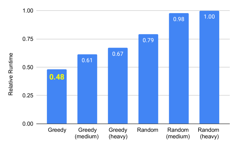
Figure 1. Average relative runtime for the greedy and random approaches (including medium and heavy variants) of parallel Leiden algorithm for all graphs in the dataset.

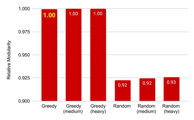
Figure 2. Average relative modularity for the greedy and random approaches (including medium and heavy variants) of parallel Leiden algorithm for all graphs in the dataset.

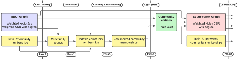
Figure 3. A flow diagram illustrating the first pass of GVE-Leiden for either a Weighted 2D-vector-based or a Weighted CSR with degree-based input graph. In the local-moving phase, vertex community memberships are updated to obtain community bounds for the refinement phase, until the cumulative delta-modularity change across all vertices reaches a specified threshold. Then, in the refinement phase, the each vertex starts in a singleton community, and community memberships are updated similarly to the local-moving phase, with vertices changing communities within their bounds. These community memberships are then counted and renumbered. In the aggregation phase, community vertices in a CSR are first obtained. This is used to create the super-vertex graph stored in a Weighted Holey CSR with degree. Subsequent passes use a Weighted Holey CSR with degree and initial community memberships for super-vertices from the previous pass as input.

4.2. Our optimized Leiden implementation

We now explain the implementation of GVE-Leiden in Algorithms 1, 2, 3, and 4. A flow diagram illustrating the first pass of GVE-Leiden is shown in Figure 3.

4.2.1. Main step of GVE-Leiden

The main step of GVE-Leiden (leiden() function) is outlined in Algorithm 1. It encompasses initialization, the local-moving phase, the refinement phase, and the aggregation phase. Here, the leiden() function accepts the input graph $G$, and returns the community membership $C$ of each vertex. In line 15, we first initialize the community membership $C$ for each vertex in $G$, and perform passes of the Leiden algorithm, limited to $MAX\_PASSES$ (lines 16-27). During each pass, we initialize the total edge weight of each vertex $K^{\prime}$, the total edge weight of each community $\Sigma^{\prime}$, and the community membership $C^{\prime}$ of each vertex in the current graph $G^{\prime}$ (line 17).

Subsequently, in line 18, we perform the local-moving phase by invoking leidenMove() (Algorithm 2), which optimizes community assignments. Following this, we set the community bound of each vertex (for the refinement phase) as the community membership of each vertex just obtained, and reset the membership of each vertex, and the total weight of each community as singleton vertices in line 19. In line 20, the refinement phase is carried out by invoking leidenRefine() (Algorithm 3), which optimizes the community assignment of each vertex within its community bound. If either the local-moving or the refinement phase converged in a single iteration, global convergence is implied and we terminate the passes (line 21). Further, if the drop in community count $|\Gamma|$ is marginal, we halt at the current pass (line 23).

If convergence has not been achieved, we proceed to renumber communities (line 24), update top-level community memberships $C$ with dendrogram lookup (line 25), perform the aggregation phase by calling leidenAggregate() (Algorithm 4), and adjust the convergence threshold for subsequent passes, i.e., perform threshold scaling (line 27). The next pass commences in line 16. At the end of all passes, we perform a final update of the top-level community memberships $C$ with dendrogram lookup (line 28), and return the top-level community membership $C$ of each vertex in $G$.

Algorithm 1 GVE-Leiden: Our parallel Leiden algorithm.

1:$G$: Input graph

2:$C$: Community membership of each vertex

3:$G^{\prime}$: Input/super-vertex graph

4:$C^{\prime}$: Community membership of each vertex in $G^{\prime}$

5:$K^{\prime}$: Total edge weight of each vertex

6:$\Sigma^{\prime}$: Total edge weight of each community

7:$G^{\prime}_{C^{\prime}}$: Community vertices (CSR)

8:$H_{t}$: Collision-free per-thread hashtable

9:$l_{i}$, $l_{j}$: Number of iterations performed (per pass)

10:$l_{p}$: Number of passes performed

11:$\tau$: Per iteration tolerance

12:$\tau_{agg}$: Aggregation tolerance

13:

14:function leiden($G$)

15:     Vertex membership: $C\leftarrow[0..|V|)$ ; $G^{\prime}\leftarrow G$

16:     for all $l_{p}\in[0..\text{\small{MAX\_PASSES}})$ do

17:         $\Sigma^{\prime}\leftarrow K^{\prime}\leftarrow vertexWeights(G^{\prime})$ ; $C^{\prime}\leftarrow[0..|V^{\prime}|)$

18:         $l_{i}\leftarrow leidenMove(G^{\prime},C^{\prime},K^{\prime},\Sigma^{\prime},\tau)$

19:         $C^{\prime}_{B}\leftarrow C^{\prime}$ ; $C^{\prime}\leftarrow[0..|V^{\prime}|)$ ; $\Sigma^{\prime}\leftarrow K^{\prime}$

20:         $l_{j}\leftarrow leidenRefine(G^{\prime},C^{\prime}_{B},C^{\prime},K^{\prime},\Sigma^{\prime},\tau)$

21:         if $l_{i}+l_{j}\leq 1$ then break $\triangleright$ Globally converged?          

22:         $|\Gamma|,|\Gamma_{old}|\leftarrow$ Number of communities in $C$, $C^{\prime}$

23:         if $|\Gamma|/|\Gamma_{old}|>\tau_{agg}$ then break $\triangleright$ Low shrink?          

24:         $C^{\prime}\leftarrow$ Renumber communities in $C^{\prime}$

25:         $C\leftarrow$ Lookup dendrogram using $C$ to $C^{\prime}$

26:         $G^{\prime}\leftarrow leidenAggregate(G^{\prime},C^{\prime})$

27:         $\tau\leftarrow\tau/\text{\small{TOLERANCE\_DROP}}$ $\triangleright$ Threshold scaling      

28:     $C\leftarrow$ Lookup dendrogram using $C$ to $C^{\prime}$

29:     return $C$

Algorithm 2 Local-moving phase of GVE-Leiden.

1:$G^{\prime}$: Input/super-vertex graph

2:$C^{\prime}$: Community membership of each vertex

3:$K^{\prime}$: Total edge weight of each vertex

4:$\Sigma^{\prime}$: Total edge weight of each community

5:$G^{\prime}_{C^{\prime}}$: Community vertices (CSR)

6:$H_{t}$: Collision-free per-thread hashtable

7:$l_{i}$: Number of iterations performed

8:$\tau$: Per iteration tolerance

9:

10:function leidenMove($G^{\prime},C^{\prime},K^{\prime},\Sigma^{\prime},\tau$)

11:     Mark all vertices in $G^{\prime}$ as unprocessed

12:     for all $l_{i}\in[0..\text{\small{MAX\_ITERATIONS}})$ do

13:         Total delta-modularity per iteration: $\Delta Q\leftarrow 0$

14:         for all unprocessed $i\in V^{\prime}$ in parallel do

15:              Mark $i$ as processed (prune)

16:              $H_{t}\leftarrow scanCommunities(\{\},G^{\prime},C^{\prime},i,false)$

17:              $\rhd$ Use $H_{t},K^{\prime},\Sigma^{\prime}$ to choose best community

18:              $c^{*}\leftarrow$ Best community linked to $i$ in $G^{\prime}$

19:              $\delta Q^{*}\leftarrow$ Delta-modularity of moving $i$ to $c^{*}$

20:              if $c^{*}=C^{\prime}[i]$ then continue               

21:              $\Sigma^{\prime}[C^{\prime}[i]]-=K^{\prime}[i]$ ; $\Sigma^{\prime}[c^{*}]+=K^{\prime}[i]$ atomic

22:              $C^{\prime}[i]\leftarrow c^{*}$ ; $\Delta Q\leftarrow\Delta Q+\delta Q^{*}$

23:              Mark neighbors of $i$ as unprocessed          

24:         if $\Delta Q\leq\tau$ then break $\triangleright$ Locally converged?               

25:     return $l_{i}$

26:

27:function scanCommunities($H_{t},G^{\prime},C^{\prime},i,self$)

28:     for all $(j,w)\in G^{\prime}.edges(i)$ do

29:         if not $self$ and $i=j$ then continue          

30:         $H_{t}[C^{\prime}[j]]\leftarrow H_{t}[C^{\prime}[j]]+w$      

31:     return $H_{t}$

Algorithm 3 Refinement phase of GVE-Leiden.

1:$G^{\prime}$: Input/super-vertex graph

2:$C^{\prime}$: Community membership of each vertex

3:$K^{\prime}$: Total edge weight of each vertex

4:$\Sigma^{\prime}$: Total edge weight of each community

5:$G^{\prime}_{C^{\prime}}$: Community vertices (CSR)

6:$H_{t}$: Collision-free per-thread hashtable

7:$l_{j}$: Number of iterations performed

8:$\tau$: Per iteration tolerance

9:

10:function leidenRefine($G^{\prime},C^{\prime}_{B},C^{\prime},K^{\prime},\Sigma^{\prime},\tau$)

11:     Mark all vertices in $G^{\prime}$ as unprocessed

12:     for all $l_{j}\in[0..\text{\small{MAX\_ITERATIONS}})$ do

13:         Total delta-modularity per iteration: $\Delta Q\leftarrow 0$

14:         for all unprocessed $i\in V^{\prime}$ in parallel do

15:              Mark $i$ as processed (prune)

16:              $H_{t}\leftarrow scanBounded(\{\},G^{\prime},C^{\prime}_{B},C^{\prime},i,false)$

17:              $\rhd$ Use $H_{t},K^{\prime},\Sigma^{\prime}$ to choose best community

18:              $c^{*}\leftarrow$ Best community linked to $i$ in $G^{\prime}$ within $C^{\prime}_{B}$

19:              $\delta Q^{*}\leftarrow$ Delta-modularity of moving $i$ to $c^{*}$

20:              if $c^{*}=C^{\prime}[i]$ then continue               

21:              $\Sigma^{\prime}[C^{\prime}[i]]-=K^{\prime}[i]$ ; $\Sigma^{\prime}[c^{*}]+=K^{\prime}[i]$ atomic

22:              $C^{\prime}[i]\leftarrow c^{*}$ ; $\Delta Q\leftarrow\Delta Q+\delta Q^{*}$

23:              Mark neighbors of $i$ as unprocessed          

24:         if $\Delta Q\leq\tau$ then break $\triangleright$ Locally converged?               

25:     return $l_{j}$

26:

27:function scanBounded($H_{t},G^{\prime},C^{\prime}_{B},C^{\prime},i,self$)

28:     for all $(j,w)\in G^{\prime}.edges(i)$ do

29:         if not $self$ and $i=j$ then continue          

30:         if $C^{\prime}_{B}[i]\neq C^{\prime}_{B}[j]$ then continue          

31:         $H_{t}[C^{\prime}[j]]\leftarrow H_{t}[C^{\prime}[j]]+w$      

32:     return $H_{t}$

Algorithm 4 Aggregation phase of GVE-Leiden.

1:$G^{\prime}$: Input/super-vertex graph

2:$C^{\prime}$: Community membership of each vertex

3:$G^{\prime}_{C^{\prime}}$: Community vertices (CSR)

4:$G^{\prime\prime}$: Super-vertex graph (weighted CSR)

5:$*.offsets$: Offsets array of a CSR graph

6:$H_{t}$: Collision-free per-thread hashtable

7:

8:function leidenAggregate($G^{\prime},C^{\prime}$)

9:     $\rhd$ Obtain vertices belonging to each community

10:     $G^{\prime}_{C^{\prime}}.offsets\leftarrow countCommunityVertices(G^{\prime},C^{\prime})$

11:     $G^{\prime}_{C^{\prime}}.offsets\leftarrow exclusiveScan(G^{\prime}_{C^{\prime}}.offsets)$

12:     for all $i\in V^{\prime}$ in parallel do

13:         Add edge $(C^{\prime}[i],i)$ to CSR $G^{\prime}_{C^{\prime}}$ atomically      

14:     $\rhd$ Obtain super-vertex graph

15:     $G^{\prime\prime}.offsets\leftarrow communityTotalDegree(G^{\prime},C^{\prime})$

16:     $G^{\prime\prime}.offsets\leftarrow exclusiveScan(G^{\prime\prime}.offsets)$

17:     $|\Gamma|\leftarrow$ Number of communities in $C^{\prime}$

18:     for all $c\in[0,|\Gamma|)$ in parallel do

19:         if degree of $c$ in $G^{\prime}_{C^{\prime}}=0$ then continue          

20:         $H_{t}\leftarrow\{\}$

21:         for all $i\in G^{\prime}_{C^{\prime}}.edges(c)$ do

22:              $H_{t}\leftarrow scanCommunities(H,G^{\prime},C^{\prime},i,true)$          

23:         for all $(d,w)\in H_{t}$ do

24:              Add edge $(c,d,w)$ to CSR $G^{\prime\prime}$ atomically               

25:     return $G^{\prime\prime}$

4.2.2. Local-moving phase of GVE-Leiden

The pseuodocode for the local-moving phase of GVE-Leiden is shown in Algorithm 2, which iteratively moves vertices between communities to maximize modularity. Here, the leidenMove() function takes the current graph $G^{\prime}$, community membership $C^{\prime}$, total edge weight of each vertex $K^{\prime}$ and each community $\Sigma^{\prime}$, the iteration tolerance $\tau$ as input, and returns the number of iterations performed $l_{i}$.

Lines 12-24 represent the main loop of the local-moving phase. In line 11, we first mark all vertices as unprocessed. Then, in line 13, we initialize the total delta-modularity per iteration $\Delta Q$. Next, in lines 14-23, we iterate over unprocessed vertices in parallel. For each unprocessed vertex $i$, we mark $i$ as processed - vertex pruning (line 15), scan communities connected to $i$ - excluding self (line 16), determine the best community $c*$ to move $i$ to (line 18), and calculate the delta-modularity of moving $i$ to $c*$ (line 19). We then update the community membership of $i$ (lines 21-22) and mark its neighbors as unprocessed (line 23) if a better community was found. In line 24, we check if the local-moving phase has converged. If so, we break out of the loop (or if $MAX\_ITERATIONS$ is reached). At the end, in line 25, we return the number of iterations performed $l_{i}$.

4.2.3. Refinement phase of GVE-Leiden

The pseuodocode for the refinement phase of GVE-Leiden is presented in Algorithm 2. This is similar to the local-moving phase, but utilizes the obtained community membership of each vertex as a community bound, where each vertex must choose to join the community of another vertex within its community bound. At the start of the refinement phase, the community membership of each vertex is reset, such that each vertex belongs to its own community. Here, the leidenRefine() function takes the current graph $G^{\prime}$, the community bound of each vertex $C^{\prime}_{B}$, the initial community membership $C^{\prime}$ of each vertex, the total edge weight of each vertex $K^{\prime}$, the initial total edge weight of each community $\Sigma^{\prime}$, and the current per iteration tolerance $\tau$ as input, and returns the number of iterations performed $l_{j}$.

Lines 12-24 represent the core of the refinement phase. First, we initialize all vertices as unprocessed (line 11). Subsequently, we initialize the per-iteration delta-modularity $\Delta Q$ (line 13), and iterate over unprocessed vertices in parallel (lines 14-23). For each unprocessed vertex $i$, we prune $i$ (line 15), scan communities connected to $i$ within the same community bound - excluding self (line 16), evaluate the best community $c*$ to move $i$ to (line 18), and compute the delta-modularity of moving $i$ to $c*$ (line 19). If a better community was found, we update the community membership (lines 21-22) of $i$, and mark its neighbors as unprocessed (line 23). In line 24, we check if the refinement phase has converged. If so, we stop iterating (or if $MAX\_ITERATIONS$ is reached). Finally, we return the number of iterations performed $l_{j}$ (line 25).

Algorithm 5 Finding disconnected communities in parallel.

1:$G$: Input graph

2:$C$: Community membership of each vertex

3:$D$: Disconnected flag for each community

4:$S$: Size of each community

5:$f_{if}$: Perform BFS to vertex $j$ if condition satisfied

6:$f_{do}$: Perform operation after each vertex is visited

7:$reached$: Number of vertices reachable from $i$ to $i$’s community

8:$work_{t}$: Work-list of current thread

9:

10:function disconnectedCommunities($G,C$)

11:     $D\leftarrow\{\}$ ; $vis\leftarrow\{\}$

12:     $S\leftarrow communitySizes(G,C)$

13:     for all threads in parallel do

14:         for all $i\in V$ do

15:              $c\leftarrow C[i]$ ; $reached\leftarrow 0$

16:              $\rhd$ Skip if community $c$ is empty, or

17:              $\rhd$ does not belong to work-list of current thread.

18:              if $S[c]=0$ or $c\notin work_{t}$ then continue               

19:              $f_{if}\leftarrow(j)\implies C[j]=c$

20:              $f_{do}\leftarrow(j)\implies reached\leftarrow reached+1$

21:              $bfsVisitForEach(vis,G,i,f_{if},f_{do})$

22:              if $reached<S[c]$ then $D[c]\leftarrow 1$               

23:              $S[c]\leftarrow 0$                

24:     return $D$

4.2.4. Aggregation phase of GVE-Leiden

Finally, we show the psuedocode for the aggregation phase in Algorithm 4, where communities are aggregated into super-vertices in preparation for the next pass of the Leiden algorithm (which operates on the super-vertex graph). Here, the leidenAggregate() function takes the current graph $G^{\prime}$ and the community membership $C^{\prime}$ as input, and returns the super-vertex graph $G^{\prime\prime}$.

In lines 10-11, the offsets array for the community vertices CSR $G^{\prime}_{C^{\prime}}.offsets$ is obtained. This is achieved by initially counting the number of vertices in each community using countCommunityVert ices() and subsequently performing an exclusive scan on the array. In lines 12-13, a parallel iteration over all vertices is performed to atomically populate vertices belonging to each community into the community graph CSR $G^{\prime}_{C^{\prime}}$. Following this, the offsets array for the super-vertex graph CSR is obtained by overestimating the degree of each super-vertex. This involves calculating the total degree of each community with communityTotalDegree() and performing an exclusive scan on the array (lines 15-16). As a result, the super-vertex graph CSR becomes holey, featuring gaps between the edges and weights arrays of each super-vertex in the CSR.

Then, in lines 18-24, a parallel iteration over all communities $c\in[0,|\Gamma|)$ is performed. For each vertex $i$ belonging to community $c$, all communities $d$ (with associated edge weight $w$), linked to $i$ as defined by scanCommunities() in Algorithm 2, are added to the per-thread hashtable $H_{t}$. Once $H_{t}$ is populated with all communities (and associated weights) linked to community $c$, these are atomically added as edges to super-vertex $c$ in the super-vertex graph $G^{\prime\prime}$. Finally, in line 25, we return the super-vertex graph $G^{\prime\prime}$.

4.3. Finding disconnected communities

We now outline our parallel algorithm for identifying disconnected communities, given the original graph and the community membership of each vertex. The core concept involves determining the size of each community, selecting a vertex from each community, traversing within the community from that vertex (avoiding adjacent communities), and marking a community as disconnected if all its vertices cannot be reached. We explore four distinct approaches, differing in the use of parallel Depth-First Search (DFS) or Breadth-First Search (BFS) and whether per-thread or shared visited flags are employed. If shared visited flags are used, each thread scans all vertices but processes only its assigned community based on the community ID. Our findings suggest that utilizing parallel BFS traversal with a shared flag vector yields the fastest results. As this is not a heuristic algorithm, all approaches produce identical outcomes. Algorithm 5 illustrates the pseudocode for this approach. Here, the disconnectedCommunities() function takes the input graph $G$ and the community membership $C$ as input, and it returns the disconnected flag $D$ for each community.

We now explain Algorithm 5 in detail. First, in line 11, the disconnected community flag $D$, and the visited vertices flags $vis$ are initialized. In line 12, the size of each community $S$ is obtained in parallel using the communitySizes() function. Subsequently, each thread processes each vertex $i$ in the graph $G$ in parallel (lines 14-23). In line 15, the community membership of $i$ ($c$) is determined, and the count of vertices reached from $i$ is initialized to $0$. If community $c$ is empty or not in the work-list of the current thread $work_{t}$, the thread proceeds to the next iteration (line 18). If however the community $c$ is non-empty and in the work-list of the current thread $work_{t}$, BFS is performed from vertex $i$ to explore vertices in the same community, using lambda functions $f_{if}$ to conditionally perform BFS to vertex $j$ if it belongs to the same community, and $f_{do}$ to update the count of $reached$ vertices after each vertex is visited during BFS (line 21). If the number of vertices $reached$ during BFS is less than the community size $S[c]$, the community $c$ is marked as disconnected (line 22). Finally, the size of the community $S[c]$ is updated to $0$, indicating that the community has been processed (line 23). Note that the work-list $work_{t}$ for each thread with ID $t$, is defined as a set containing communities $[t\chi,\ t(\chi+1))\ \cup\ [T\chi+t\chi,\ T\chi+t(\chi+1))\ \cup\ \ldots$, where $\chi$ is the chunk size, and $T$ is the number of threads. We use a chunk size of $\chi=1024$.

5. Evaluation

5.1. Experimental Setup

5.1.1. System used

We employ a server equipped with two Intel Xeon Gold 6226R processors, each featuring $16$ cores running at a clock speed of $2.90$ GHz. Each core is equipped with a $1$ MB L1 cache, a $16$ MB L2 cache, and a $22$ MB shared L3 cache. The system is configured with $376$ GB RAM and set up with CentOS Stream 8.

5.1.2. Configuration

We use 32-bit integers for vertex ids and 32-bit float for edge weights but use 64-bit floats for computations and hashtable values. We utilize $64$ threads to match the number of cores available on the system (unless specified otherwise). For compilation, we use GCC 8.5 and OpenMP 4.5.

5.1.3. Dataset

The graphs used in our experiments are given in Table 1. These are sourced from the SuiteSparse Matrix Collection (Kolodziej et al., 2019). In the graphs, number of vertices vary from $3.07$ to $214$ million, and number of edges vary from $25.4$ million to $3.80$ billion. We ensure edges to be undirected and weighted with a default of $1$.

Table 1. List of $13$ graphs obtained SuiteSparse Matrix Collection (Kolodziej et al., 2019) (directed graphs are marked with $*$). Here, $|V|$ is the number of vertices, $|E|$ is the number of edges (after adding reverse edges), $D_{avg}$ is the average degree, and $|\Gamma|$ is the number of communities obtained with GVE-Leiden.

Graph	$|V|$	$|E|$	$D_{avg}$	$|\Gamma|$
Web Graphs (LAW)
indochina-2004∗	7.41M	341M	41.0	5.00K
uk-2002∗	18.5M	567M	16.1	43.1K
arabic-2005∗	22.7M	1.21B	28.2	3.80K
uk-2005∗	39.5M	1.73B	23.7	21.2K
webbase-2001∗	118M	1.89B	8.6	2.77M
it-2004∗	41.3M	2.19B	27.9	5.24K
sk-2005∗	50.6M	3.80B	38.5	3.75K
Social Networks (SNAP)
com-LiveJournal	4.00M	69.4M	17.4	2.33K
com-Orkut	3.07M	234M	76.2	33
Road Networks (DIMACS10)
asia_osm	12.0M	25.4M	2.1	2.56K
europe_osm	50.9M	108M	2.1	3.61K
Protein k-mer Graphs (GenBank)
kmer_A2a	171M	361M	2.1	19.4K
kmer_V1r	214M	465M	2.2	8.60K

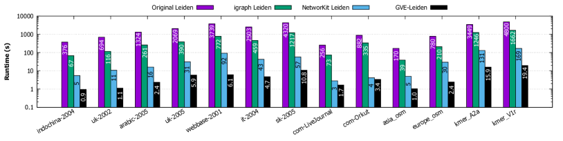
(a) Runtime in seconds (logarithmic scale) with Original Leiden, igraph Leiden, NetworKit Leiden, and GVE-Leiden

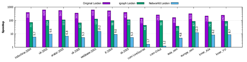
(b) Speedup of GVE-Leiden (logarithmic scale) with respect to Original Leiden, igraph Leiden, NetworKit Leiden.

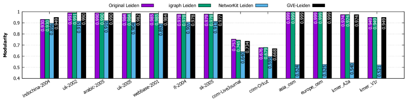
(c) Modularity of communities obtained with Original Leiden, igraph Leiden, NetworKit Leiden, and GVE-Leiden.

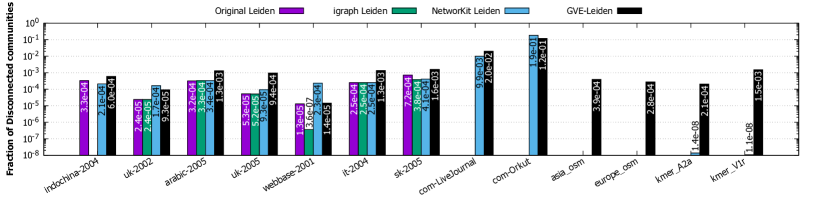
(d) Fraction of disconnected communities (logarithmic scale) with Original Leiden, igraph Leiden, NetworKit Leiden, and GVE-Leiden.

Figure 4. Runtime in seconds (log-scale), speedup (log-scale), modularity, and fraction of disconnected communities (log-scale) with Original Leiden, igraph Leiden, NetworKit Leiden, and GVE-Leiden for each graph in the dataset.

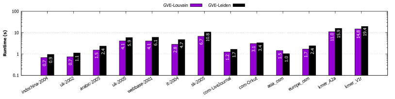
(a) Runtime in seconds (logarithmic scale) with GVE-Louvain and GVE-Leiden

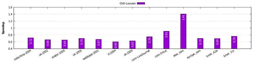
(b) Speedup of GVE-Leiden with respect to GVE-Louvain. GVE-Leiden is generally slower (speedup ¡ $1$) because of additional refinement phase.

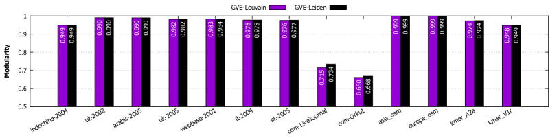
(c) Modularity of communities obtained with GVE-Louvain and GVE-Leiden.

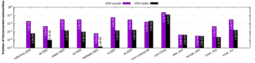
(d) Fraction of disconnected communities (logarithmic scale) with GVE-Louvain and GVE-Leiden.

Figure 5. Runtime in seconds (log-scale), speedup, modularity, and fraction of disconnected communities (log-scale) with GVE-Louvain and GVE-Leiden for each graph in the dataset.

5.2. Comparing Performance of GVE-Leiden

We now compare the performance of GVE-Leiden with the original Leiden (Traag et al., 2019), igraph Leiden (Csardi et al., 2006), and NetworKit Leiden (Staudt et al., 2016). For the original Leiden, we use a C++ program to initialize a ModularityVertexPartition upon the loaded graph, and invoke optimise_partition() to obtain the community membership of each vertex in the graph. For igraph Leiden, we use igraph_commun ity_leiden() with a resolution of $1/2|E|$, a beta of $0.01$, and request the algorithm to run until convergence. For NetworKit Leiden, we write a Python script to call ParallelLeiden(), while limiting the number of passes to $10$. For each graph, we measure the runtime of each implementation and the modularity of the communities obtained, five times, for averaging. We also save the community membership vector to a file and later count the number of disconnected components using Algorithm 5. In all instances, we use modularity as the quality function to optimize for.

Figure 4(a) shows the runtimes of the original Leiden, igraph Leiden, NetworKit Leiden, and GVE-Leiden on each graph in the dataset. On the sk-2005 graph, GVE-Leiden finds communities in $10.8$ seconds, and thus achieve a processing rate of $352$ million edges/s. Figure 4(b) shows the speedup of GVE-Leiden with respect to each implementation mentioned above. GVE-Leiden is on average $373\times$, $86\times$, and $7.2\times$ faster than the original Leiden, igraph Leiden, and NetworKit Leiden respectively. Figure 4(c) shows the modularity of communities obtained with each implementation. GVE-Leiden on average obtains $0.1\%$ lower modularity than the original Leiden and igraph Leiden, and $26\%$ higher modularity than NetworKit Leiden (especially on road networks and protein k-mer graphs). Finally, Figure 4(d) shows the fraction of disconnected communities obtained with each implementation. Here, the absence of bars indicates the absence of disconnected communities. Communities identified by GVE-Leiden on average have $88\times$, $145\times$, and $0.76\times$ disconnected communities than the original Leiden, igraph Leiden, and NetworKit Leiden respectively. While this compares unfavorably with the original Leiden and igraph Leiden (especially on social networks, road networks, and protein k-mer graphs), it may be simpler to split the disconnected communities obtained from GVE-Leiden as a post-processing step. We would like to address this issue some time in the future.

Next, we compare the performance of GVE-Leiden with GVE-Louvain (Sahu, 2023), our parallel implementation of the Louvain method. As above, for each graph in the dataset, we run both algorithms 5 times to minimize measurement noise. Figure 5(a) shows the runtimes of GVE-Louvain and GVE-Leiden on each graph in the dataset. Figure 5(b) shows the speedup of GVE-Leiden with respect to GVE-Louvain. GVE-Leiden is on average $36\%$ slower than GVE-Louvain. This increase in computation time is a trade-off for obtaining significantly fewer disconnected communities, as given below. Figure 5(c) shows the modularity of communities obtained with GVE-Louvain and GVE-Leiden. GVE-Leiden on average obtains $0.3\%$ higher modularity than GVE-Louvain. Finally, Figure 5(d) shows the fraction of internally-disconnected communities obtained with GVE-Louvain and GVE-Leiden. Communities identified by GVE-Leiden on average have an $11$-fold decrease in the number of disconnected communities than GVE-Louvain.

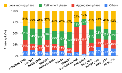
(a) Phase split

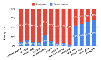
(b) Pass split

Figure 6. Phase split of GVE-Leiden shown on the left, and pass split shown on the right for each graph in the dataset.

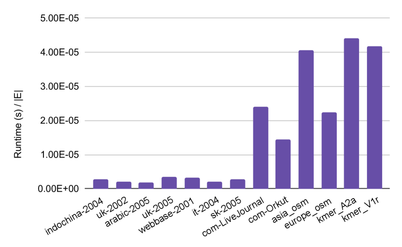
Figure 7. Runtime $/|E|$ factor with GVE-Leiden for each graph in the dataset.

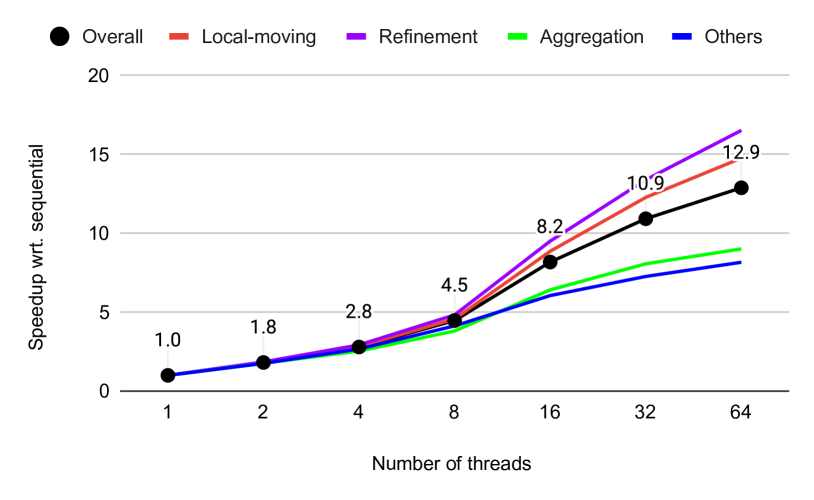
Figure 8. Overall speedup of GVE-Leiden, and its various phases (local-moving, refinement, aggregation, others), with increasing number of threads (in multiples of 2).

5.3. Analyzing Performance of GVE-Leiden

We now analyze the performance of GVE-Leiden. The phase-wise and pass-wise split of GVE-Leiden is shown in Figures 6(a) and 6(b) respectively. Figure 6(a) reveals that GVE-Leiden devotes a significant portion of its runtime to the local-moving and refinement phases on web graphs, road networks, and protein k-mer graphs, while it dedicates majority of its runtime in the aggregation phase on social networks. The pass-wise split, shown in Figure 6(b), indicates that the first pass is time-intensive for high-degree graphs (web graphs and social networks), while subsequent passes take precedence in execution time on low-degree graphs (road networks and protein k-mer graphs).

On average, GVE-Leiden spends $37\%$ of its runtime in the local-moving phase, $27\%$ in the refinement phase, $24\%$ in the aggregation phase, and $12\%$ in other steps (initialization, renumbering communities, dendrogram lookup, and resetting communities). Further, $73\%$ of the runtime is consumed by the first pass of the algorithm, which is computationally demanding due to the size of the original graph (subsequent passes operate on super-vertex graphs). We also observe that graphs with lower average degree (road networks and protein k-mer graphs) and those with poor community structure (e.g., com-LiveJournal and com-Orkut) exhibit a higher $\text{runtime}/|E|$ factor, as shown in Figure 7.

5.4. Strong Scaling of GVE-Leiden

Finally, we assess the strong scaling performance of GVE-Leiden. In this analysis, we vary the number of threads from $1$ to $64$ in multiples of $2$ for each input graph, and measure the total time taken for GVE-Leiden to identify communities, encompassing its phase splits (local-moving, refinement, aggregation, and others), repeated five times for averaging. The results are shown in Figure 8. With 32 threads, GVE-Leiden achieves an average speedup of $10.9\times$ compared to a single-threaded execution, indicating a performance increase of $1.6\times$ for every doubling of threads. Nevertheless, scalability is restricted due to the sequential nature of steps/phases in the algorithm. At 64 threads, GVE-Leiden is affected by NUMA effects, resulting in a speedup of only $12.9\times$.

6. Conclusion

In conclusion, this study addresses the design of an optimized parallel implementation of the Leiden algorithm (Traag et al., 2019), a high-quality community detection algorithm that improves upon the popular Louvain method (Blondel et al., 2008), in the shared memory setting. We extend optimizations for the Louvain algorithm (Sahu, 2023) to our implementation of the Leiden algorithm, and use a greedy refinement phase where vertices greedily optimize for delta-modularity within their community bounds, which we observe, offers both better performance and quality than a randomized approach.

On a system equipped with two 16-core Intel Xeon Gold 6226R processors, our implementation of the Leiden algorithm, referred to as GVE-Leiden, attains a processing rate of $352M$ edges per second on a $3.8B$ edge graph. It surpasses the original Leiden implementation, igraph Leiden, and NetworKit Leiden by factors of $373\times$, $86\times$, and $7.2\times$ respectively. GVE-Leiden identifies communities of equivalent quality to the first two implementations, and $26\%$ higher quality than NetworKit. Doubling the number of threads results in an average performance scaling of $1.6\times$ for GVE-Leiden. In comparison to GVE-Louvain (Sahu, 2023), our parallel Louvain implementation, GVE-Leiden reduces internally-disconnected communities by a factor of $11$ with only a $36\%$ increase in runtime.

However, on average, communities identified by GVE-Leiden exhibit $88\times$, $145\times$, and $0.76\times$ more disconnected communities compared to the original Leiden, igraph Leiden, and NetworKit Leiden, respectively. This disparity is particularly noticeable on social networks, road networks, and protein k-mer graphs. Despite this drawback, a potential solution is to address the issue by post-processing, where disconnected communities obtained from GVE-Leiden can be split. We acknowledge this concern, and plan to explore solutions in future work.

- (1)
- Aldabobi et al. (2022) A. Aldabobi, A. Sharieh, and R. Jabri. 2022. An improved Louvain algorithm based on Node importance for Community detection. Journal of Theoretical and Applied Information Technology 100, 23 (2022), 1–14.
- Blondel et al. (2008) V. Blondel, J. Guillaume, R. Lambiotte, and E. Lefebvre. 2008. Fast unfolding of communities in large networks. Journal of Statistical Mechanics: Theory and Experiment 2008, 10 (Oct 2008), P10008.
- Brandes et al. (2007) U. Brandes, D. Delling, M. Gaertler, R. Gorke, M. Hoefer, Z. Nikoloski, and D. Wagner. 2007. On modularity clustering. IEEE transactions on knowledge and data engineering 20, 2 (2007), 172–188.
- Cheong et al. (2013) C. Cheong, H. Huynh, D. Lo, and R. Goh. 2013. Hierarchical Parallel Algorithm for Modularity-Based Community Detection Using GPUs. In Proceedings of the 19th International Conference on Parallel Processing (Aachen, Germany) (Euro-Par’13). Springer-Verlag, Berlin, Heidelberg, 775–787.
- Csardi et al. (2006) G. Csardi, T. Nepusz, et al. 2006. The igraph software package for complex network research. InterJournal, complex systems 1695, 5 (2006), 1–9.
- Fazlali et al. (2017) M. Fazlali, E. Moradi, and H. Malazi. 2017. Adaptive parallel Louvain community detection on a multicore platform. Microprocessors and microsystems 54 (Oct 2017), 26–34.
- Gach and Hao (2014) O. Gach and J. Hao. 2014. Improving the Louvain algorithm for community detection with modularity maximization. In Artificial Evolution: 11th International Conference, Evolution Artificielle, EA , Bordeaux, France, October 21-23, . Revised Selected Papers 11. Springer, Springer, Bordeaux, France, 145–156.
- Ghosh et al. (2019) S. Ghosh, M. Halappanavar, A. Tumeo, and A. Kalyanarainan. 2019. Scaling and quality of modularity optimization methods for graph clustering. In IEEE High Performance Extreme Computing Conference (HPEC). IEEE, 1–6.
- Ghosh et al. (2018) S. Ghosh, M. Halappanavar, A. Tumeo, A. Kalyanaraman, H. Lu, D. Chavarria-Miranda, A. Khan, and A. Gebremedhin. 2018. Distributed louvain algorithm for graph community detection. In IEEE International Parallel and Distributed Processing Symposium (IPDPS). Vancouver, British Columbia, Canada, 885–895.
- Gregory (2010) S. Gregory. 2010. Finding overlapping communities in networks by label propagation. New Journal of Physics 12 (10 2010), 103018. Issue 10.
- Halappanavar et al. (2017) M. Halappanavar, H. Lu, A. Kalyanaraman, and A. Tumeo. 2017. Scalable static and dynamic community detection using Grappolo. In IEEE High Performance Extreme Computing Conference (HPEC). IEEE, Waltham, MA USA, 1–6.
- Kolodziej et al. (2019) S. Kolodziej, M. Aznaveh, M. Bullock, J. David, T. Davis, M. Henderson, Y. Hu, and R. Sandstrom. 2019. The SuiteSparse matrix collection website interface. The Journal of Open Source Software 4, 35 (Mar 2019), 1244.
- Lancichinetti and Fortunato (2009) A. Lancichinetti and S. Fortunato. 2009. Community detection algorithms: a comparative analysis. Physical Review. E, Statistical, Nonlinear, and Soft Matter Physics 80, 5 Pt 2 (Nov 2009), 056117.
- Leskovec (2021) J. Leskovec. 2021. CS224W: Machine Learning with Graphs — 2021 — Lecture 13.3 - Louvain Algorithm. https://www.youtube.com/watch?v=0zuiLBOIcsw
- Lu et al. (2015) H. Lu, M. Halappanavar, and A. Kalyanaraman. 2015. Parallel heuristics for scalable community detection. Parallel computing 47 (Aug 2015), 19–37.
- Mohammadi et al. (2020) M. Mohammadi, M. Fazlali, and M. Hosseinzadeh. 2020. Accelerating Louvain community detection algorithm on graphic processing unit. The Journal of supercomputing (Nov 2020).
- Naim et al. (2017) M. Naim, F. Manne, M. Halappanavar, and A. Tumeo. 2017. Community detection on the GPU. In IEEE International Parallel and Distributed Processing Symposium (IPDPS). IEEE, Orlando, Florida, USA, 625–634.
- Newman (2006) M. Newman. 2006. Finding community structure in networks using the eigenvectors of matrices. Physical review E 74, 3 (2006), 036104.
- Nguyen ([n. d.]) Fabian Nguyen. [n. d.]. Leiden-Based Parallel Community Detection. Bachelor’s Thesis. Karlsruhe Institute of Technology, 2021 (zitiert auf S. 31).
- Ozaki et al. (2016) N. Ozaki, H. Tezuka, and M. Inaba. 2016. A simple acceleration method for the Louvain algorithm. International Journal of Computer and Electrical Engineering 8, 3 (2016), 207.
- Que et al. (2015) X. Que, F. Checconi, F. Petrini, and J. Gunnels. 2015. Scalable community detection with the louvain algorithm. In IEEE International Parallel and Distributed Processing Symposium. IEEE, IEEE, Hyderabad, India, 28–37.
- Rotta and Noack (2011) R. Rotta and A. Noack. 2011. Multilevel local search algorithms for modularity clustering. Journal of Experimental Algorithmics (JEA) 16 (2011), 2–1.
- Ryu and Kim (2016) S. Ryu and D. Kim. 2016. Quick community detection of big graph data using modified louvain algorithm. In IEEE 18th International Conference on High Performance Computing and Communications (HPCC). IEEE, Sydney, NSW, 1442–1445.
- Sahu (2023) Subhajit Sahu. 2023. GVE-Louvain: Fast Louvain Algorithm for Community Detection in Shared Memory Setting. arXiv preprint arXiv:2312.04876 (2023).
- Sattar and Arifuzzaman (2019) N. Sattar and S. Arifuzzaman. 2019. Overcoming MPI Communication Overhead for Distributed Community Detection. In Software Challenges to Exascale Computing, A. Majumdar and R. Arora (Eds.). Springer Singapore, Singapore, 77–90.
- Shi et al. (2021) J. Shi, L. Dhulipala, D. Eisenstat, J. Ł\kacki, and V. Mirrokni. 2021. Scalable community detection via parallel correlation clustering.
- Staudt et al. (2016) C.L. Staudt, A. Sazonovs, and H. Meyerhenke. 2016. NetworKit: A tool suite for large-scale complex network analysis. Network Science 4, 4 (2016), 508–530.
- Traag (2015) V. Traag. 2015. Faster unfolding of communities: Speeding up the Louvain algorithm. Physical Review E 92, 3 (2015), 032801.
- Traag et al. (2011) V. Traag, P. Dooren, and Y. Nesterov. 2011. Narrow scope for resolution-limit-free community detection. Physical Review E 84, 1 (2011), 016114.
- Traag et al. (2019) V. Traag, L. Waltman, and N. Eck. 2019. From Louvain to Leiden: guaranteeing well-connected communities. Scientific Reports 9, 1 (Mar 2019), 5233.
- Verweij ([n. d.]) Geerten Verweij. [n. d.]. Faster Community Detection Without Loss of Quality: Parallelizing the Leiden Algorithm. Master’s Thesis. Leiden University, 2020.
- Waltman and Eck (2013) L. Waltman and N. Eck. 2013. A smart local moving algorithm for large-scale modularity-based community detection. The European physical journal B 86, 11 (2013), 1–14.
- Wickramaarachchi et al. (2014) C. Wickramaarachchi, M. Frincu, P. Small, and V. Prasanna. 2014. Fast parallel algorithm for unfolding of communities in large graphs. In IEEE High Performance Extreme Computing Conference (HPEC). IEEE, IEEE, Waltham, MA USA, 1–6.
- You et al. (2022) Y. You, L. Ren, Z. Zhang, K. Zhang, and J. Huang. 2022. Research on improvement of Louvain community detection algorithm. In 2nd International Conference on Artificial Intelligence, Automation, and High-Performance Computing (AIAHPC ), Vol. 12348. SPIE, Zhuhai, China, 527–531.
- Zhang et al. (2021) J. Zhang, J. Fei, X. Song, and J. Feng. 2021. An improved Louvain algorithm for community detection. Mathematical Problems in Engineering 2021 (2021), 1–14.