Towards consistent nuclear interactions from chiral Lagrangians II:
Symmetry preserving regularization

Abstract

Low-energy nuclear structure and reactions can be described in a systematically improvable way using the framework of chiral effective field theory. This requires solving the quantum mechanical many-body problem with regularized nuclear forces and current operators, derived from the most general effective chiral Lagrangian. To maintain the chiral and gauge symmetries, a symmetry preserving cutoff regularization has to be employed when deriving nuclear potentials. Here, we discuss various regularization techniques and show how this task can be accomplished by regularizing the pion field in the effective chiral Lagrangian using the gradient flow method. The actual derivation of the nuclear forces and currents from the regularized effective Lagrangian can be carried out utilizing the novel path-integral approach introduced in our earlier paper.

I Introduction

Dimensional regularization (DR) is a commonly used method to treat ultraviolet divergent loop integrals in quantum field theory. Its usefulness rests on its computational efficiency and the fact that this method preserves the relevant symmetries such as the chiral and gauge ones. However, while being highly convenient in the realm of perturbation theory, DR can usually not be employed in nonperturbative calculations, especially if results are only available numerically as it is, e.g., the case in applications of chiral effective field theory (EFT) to nuclear systems. Here, observables are calculated by a numerical solution of the $A$-body Schrödinger equation using (highly singular) potentials derived from the effective chiral Lagrangian, see Refs. Epelbaum:2008ga ; Machleidt:2011zz for review articles. The (unphysical) singular short-distance behavior of such potentials reflects their effective nature, and it is usually dealt with by introducing some kind of cutoff regulator in the Schrödinger equation. Renormalization then ensures that the calculated low-energy observables are insensitive to regularization details at the accuracy level of the EFT expansion Gasparyan:2021edy ; Gasparyan:2023rtj .

In Refs. Epelbaum:2019kcf ; Krebs:2019uvm , we pointed out that the commonly used approach to regularize pion-exchange potentials by multiplying the expressions, derived in chiral EFT using momentum-independent regularization schemes such as DR, with some cutoff functions is inconsistent as it violates chiral symmetry when applied to three- and more-nucleon systems and/or processes involving external probes. The inconsistency originates from mixing the two different regularization schemes. It can be avoided by re-deriving nuclear potentials using cutoff regularization instead of DR. The purpose of this paper is to discuss in detail symmetry-preserving regularization of the effective chiral Lagrangian, which is suitable for the derivation of regularized nuclear interactions from chiral EFT. Specifically, we focus here on cutoff regularization of the pion and/or pion-nucleon Lagrangians $\mathcal{L}_{\pi}$ and $\mathcal{L}_{\pi N}$, respectively, and we seek for a scheme that (i) preserves the chiral and gauge symmetries, (ii) reduces to the Gaussian-type regulator of Ref. Reinert:2017usi when applied to the one-pion exchange two-nucleon potential and (iii) results in finite pion-exchange contributions to the nuclear forces and current operators (at least if used in combination with DR or $\zeta$-function regularization), which are non-singular at short distances (i.e., sufficiently regularized). We emphasize that at the accuracy level of chiral EFT we aim for, regularization of few-nucleon contact interactions does not require additional efforts to maintain the chiral symmetry. The regularized chiral Lagrangian constructed in this paper can be employed to derive consistent nuclear interactions using the path-integral approach introduced in Ref. Krebs:2023ljo .

Our paper is organized as follows. First, in sec. II we briefly remind the reader of the main idea behind the higher-derivative method introduced by Slavnov to regularize the non-linear $\sigma$-model Slavnov:1971aw before DR was invented, see also Refs. Djukanovic:2004px ; Long:2016vnq for a related work. We also show in this section that a naive application of this method to the problem at hand fails because of deregularization of multi-pion interactions. This issue can be mitigated by choosing all cutoff-dependent terms in the effective Lagrangian to be proportional to the equation of motion (EOM), as done in the original work by Slavnov Slavnov:1971aw . In sec. III, we consider such an ansatz for the regularized pion Lagrangian and show that it indeed leads to satisfactory results as far as nuclear forces are concerned. However, when applied to the electromagnetic current operator, this scheme leads to certain badly divergent loop integrals with exponentially growing integrands, signalling that the considered ansatz is still insufficient for our purposes. An alternative approach to regularize the pion field using the gradient flow method has been suggested by Kaplan Kaplan and is considered in sec. IV. We work out the explicit form of the regularized effective Lagrangian and show that this scheme yields finite and regularized expressions for the nuclear forces and currents, thereby fulfilling all demanded criteria. The main results of our paper are summarized in sec. V, while appendices A, B and C provide details on the derivation of the four-nucleon force considered in the main text, the equation of motion (EOM) for pion fields and the regularized Lagrangian using the ansatz of sec. III. Finally, appendix D describes the proof that the chiral transformation properties of the generalized pion field in the gradient flow method do not depend on the flow parameter.

II Higher derivative regularization

We start with the effective chiral Lagrangian, which can be conveniently written in terms of the $\rm SU(2)$ matrix $U$ that collects the pion fields and transforms with respect to the chiral $\rm SU(2)_{L}\times SU(2)_{R}$ rotations according to $U\to RUL^{\dagger}$. Here and in what follows, we use the standard notation by introducing the building blocks Bernard:1995dp

$$u = \sqrt{U},\quad\quad u_{\mu}\,=\,iu^{\dagger}\nabla_{\mu}Uu^{\dagger},\quad\quad\nabla_{\mu}U\,=\,\partial_{\mu}U-ir_{\mu}U+iUl_{\mu},\quad\quad D_{\mu}\,=\,\partial_{\mu}+\Gamma_{\mu},$$

$$\Gamma_{\mu} = \frac{1}{2}\big{[}u^{\dagger},\partial_{\mu}u\big{]}-\frac{i}{2}u^{\dagger}r_{\mu}u-\frac{i}{2}u\,l_{\mu}u^{\dagger},\quad\quad\chi_{\pm}\,=\,u^{\dagger}\chi\,u^{\dagger}\pm u\,\chi^{\dagger}u,\quad\quad\chi\,=\,2B(s+ip),$$ (2.1)

where $\Gamma_{\mu}$ is the chiral connection, $l_{\mu}$, $r_{\mu}$, $s$ and $p$ refer to left-handed, right-handed, scalar and pseudoscalar external sources, respectively, while $B$ is a low-energy constant. Throughout this paper, we neglect isospin-breaking corrections and set the external scalar source $s$ to a constant value equal to the average mass of the up- and down-quarks, $s=m_{q}$.

To derive nuclear potentials using the path-integral method of Ref. Krebs:2023ljo , we have to switch to Euclidean space. The lowest-order pion Lagrangian has the well-known form

$${\cal L}_{\pi}^{\rm E\,(2)}=\frac{F^{2}}{4}{\rm Tr}\big{[}u_{\mu}u_{\mu}-\chi_{+}\big{]}\,=\,\frac{F^{2}}{4}{\rm Tr}\big{[}\big{(}\nabla_{\mu}U\big{)}^{\dagger}\nabla_{\mu}U-U^{\dagger}\chi-\chi^{\dagger}U\big{]}\,,$$ (2.2)

where $F$ is the pion decay constant in the chiral limit. The superscripts $\rm E$ and $(2)$ signify that the Lagrangian is written in Euclidean space and that it involves terms with two derivatives or a single insertion of the quark mass $m_{q}$, respectively.

Our goal is to modify the effective Lagrangian by introducing a momentum-space cutoff in a symmetry-preserving manner to ensure that all pion-exchange contributions to the nuclear potentials and currents get sufficiently regularized with respect to the external momenta of the nucleons. As already pointed out in our earlier papers Epelbaum:2019kcf ; Krebs:2019uvm ; Krebs:2020plh ; Epelbaum:2022cyo , the higher derivative method of Ref. Slavnov:1971aw provides a promising approach to achieve this goal. The main idea behind this method is to modify the Lagrangian by including certain higher-order terms, chosen to improve the ultraviolet behavior of loop integrals that appear in the calculation of the scattering amplitude. Below, we demonstrate this idea by considering an explicit example, and we also point out some subtleties that occur in a naive application of this scheme. For the sake of simplicity, we switch off all external sources and consider the chiral limit of $m_{q}=0$ throughout this section.

Inspired by the original work by Slavnov Slavnov:1971aw , we intend to improve the ultraviolet behavior of the pion propagator by modifying the Lagrangian via:

$${\cal L}_{\pi}^{\rm E\,(2)} = \frac{F^{2}}{4}{\rm Tr}\Big{[}\partial_{\mu}U^{\dagger}\partial_{\mu}U\Big{]}\,\,\longrightarrow\,\,{\cal L}_{\pi,\Lambda}^{\rm E\,(2)}\,=\,\frac{F^{2}}{4}{\rm Tr}\bigg{[}\partial_{\mu}U^{\dagger}e^{-\partial^{2}/\Lambda^{2}}\partial_{\mu}U\bigg{]},$$ (2.3)

where $\Lambda$ is a momentum cutoff. The choice of the modification is obviously not unique: while Ref. Slavnov:1971aw included terms polynomial in $\partial^{2}$, the modification in Eq. (2.3) is chosen to match the regularized one-pion exchange two-nucleon potential of Refs. Reinert:2017usi ; Reinert:2020mcu . However, we will show below that the ansatz in Eq. (2.3) does not provide a sufficient regularization for certain type of contributions to the nuclear forces and is, therefore, not sufficient for our purposes.

To proceed with the calculation, we employ the so-called $\sigma$-gauge parametrization of the matric $U$ in terms of the pion field $\pi$,

$$U = \sqrt{1-\frac{\mbox{\boldmath$\pi$}^{2}}{F^{2}}}+i\frac{\mbox{\boldmath$\tau$}\cdot\mbox{\boldmath$\pi$}}{F}\,,$$ (2.4)

where $\tau$ refer to the isospin Pauli matrices. Then, the regularized Lagrangian of Eq. (2.3), expanded in powers of the pion field, takes the form:

$${\cal L}_{\pi,\Lambda}^{\rm E\,(2)} = -\frac{1}{2}\mbox{\boldmath$\pi$}\cdot\partial^{2}\,e^{-\partial^{2}/\Lambda^{2}}\mbox{\boldmath$\pi$}+\frac{1}{2F^{2}}\mbox{\boldmath$\pi$}\cdot\partial_{\mu}\mbox{\boldmath$\pi$}\,e^{-\partial^{2}/\Lambda^{2}}\mbox{\boldmath$\pi$}\cdot\partial_{\mu}\mbox{\boldmath$\pi$}+{\cal O}(\pi^{6}).$$ (2.5)

The first term can be rewritten in terms of the inverse pion propagator. As desired, the exponentially growing (in momentum space) factor in this term improves the ultraviolet behavior of the pion propagator in Euclidean space, which takes the form (in the chiral limit)

$$\Delta^{\rm E}(x_{i}-x_{j})\,=\,\int\frac{d^{4}q}{(2\pi)^{4}}e^{iq\cdot(x_{i}-x_{j})}\,\frac{e^{-(q_{0}^{2}+\vec{q}^{\,2})/\Lambda^{2}}}{q_{0}^{2}+\vec{q}^{\,2}}.$$ (2.6)

However, from Eq. (2.5) we see that also interactions involving four and more pion fields acquire exponential factors that grow with increasing momenta. Such factors are problematic from the regularization point of view as can already be seen from tree-level diagrams involving the four-pion vertex. In Fig. 1, we show selected contributions to the four-nucleon force (4NF) at fourth order (N³LO) in chiral EFT.

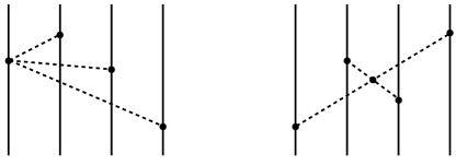
Figure 1: Representation invariant class of diagrams that contribute to the four-nucleon force at N³LO. Solid and dashed lines refer to nucleons and pions, respectively. Solid dots denote the lowest-order vertices from the effective chiral Lagrangian.

A complete set of diagrams and the corresponding unregularized expressions for the 4NF, calculated using the method of unitary transformation Epelbaum:1998ka , can be found in Refs. Epelbaum:2005bjv ; Epelbaum:2007us . Notice that while the contribution of each of the shown Feynman diagrams depends on the parametrization of the SU(2) matrix $U$, their sum is representation invariant. Since the first diagram does not involve any vertices from ${\cal L}_{\pi,\Lambda}^{\rm E\,(2)}$, its contribution can be read off from the corresponding unregularized result by simply replacing all pion propagators with the regularized ones given in Eq. (2.6). More interesting is the 4NF contribution stemming from the second diagram in Fig. 1. In Ref. Krebs:2023ljo , we have introduced a general method to derive nuclear forces and currents from regularized effective Lagrangians using the path-integral formalism. However, since the diagram we are interested in does not involve reducible pieces, the expression for the 4NF coincides with the one for the scattering amplitude and can be easily obtained using the standard Feynman diagram technique. A straightforward calculation using the lowest-order pion-nucleon Lagrangian, along with the regularized Lagrangian ${\cal L}_{\pi,\Lambda}^{\rm E\,(2)}$ of Eq. (2.5) yields the following result for the second graph in Fig. 1 (in the chiral limit):

$$V^{4N}_{\Lambda} = \frac{g^{4}}{128F^{6}}\mbox{\boldmath$\tau$}_{1}\cdot\mbox{\boldmath$\tau$}_{2}\mbox{\boldmath$\tau$}_{3}\cdot\mbox{\boldmath$\tau$}_{4}\,\frac{\vec{\sigma}_{1}\cdot\vec{q}_{1}\vec{\sigma}_{2}\cdot\vec{q}_{2}\vec{\sigma}_{3}\cdot\vec{q}_{3}\vec{\sigma}_{4}\cdot\vec{q}_{4}}{\vec{q}_{1}^{\,2}\,\vec{q}_{2}^{\,2}\,\vec{q}_{3}^{\,2}\,\vec{q}_{4}^{\,2}}\,\vec{q}_{12}^{\,2}\,e^{-\frac{\vec{q}_{1}^{\,2}}{\Lambda^{2}}}\,e^{-\frac{\vec{q}_{2}^{\,2}}{\Lambda^{2}}}\,e^{-\frac{\vec{q}_{3}^{\,2}}{\Lambda^{2}}}\,e^{-\frac{\vec{q}_{4}^{\,2}}{\Lambda^{2}}}\,e^{\frac{\vec{q}_{12}^{\,2}}{\Lambda^{2}}}\,+\,23\text{ perm.}$$ (2.7)

$$= \frac{g^{4}}{128F^{6}}\mbox{\boldmath$\tau$}_{1}\cdot\mbox{\boldmath$\tau$}_{2}\mbox{\boldmath$\tau$}_{3}\cdot\mbox{\boldmath$\tau$}_{4}\,\frac{\vec{\sigma}_{1}\cdot\vec{q}_{1}\vec{\sigma}_{2}\cdot\vec{q}_{2}\vec{\sigma}_{3}\cdot\vec{q}_{3}\vec{\sigma}_{4}\cdot\vec{q}_{4}}{\vec{q}_{1}^{\,2}\,\vec{q}_{2}^{\,2}\,\vec{q}_{3}^{\,2}\,\vec{q}_{4}^{\,2}}\,\vec{q}_{12}^{\,2}\,e^{-\frac{\vec{q}_{13}^{\,2}}{\Lambda^{2}}}e^{-\frac{\vec{q}_{14}^{\,2}}{\Lambda^{2}}}\,+\,23\text{ perm.},$$

where we have dropped the prefactor $(2\pi)^{3}\delta(\vec{q}_{1}+\vec{q}_{2}+\vec{q}_{3}+\vec{q}_{4})$ following the standard convention for nuclear potentials. Here, $\vec{\sigma}_{i}$ and $\vec{q}_{i}=\vec{p}_{i}^{\,\prime}-\vec{p}_{i}$ denote the Pauli spin matrices and the momentum transfer of nucleon $i$, respectively, while $\vec{q}_{ij}\equiv\vec{q}_{i}+\vec{q}_{j}$. Further, $g$ denotes the nucleon axial vector coupling in the chiral limit. To obtain the last equality in Eq. (2.7), we have used the obvious relationship $\vec{q}_{1}+\vec{q}_{2}+\vec{q}_{3}+\vec{q}_{4}=0$. When removing the regulator by taking the limit $\Lambda\to\infty$, the above expression reduces to the chiral-limit version of Eq. (3.44) of Ref. Epelbaum:2007us if one sets $\alpha=0$ to comply with the $\sigma$-gauge parametrization in Eq. (2.4). From Eq. (2.7), we see that the resulting four-nucleon force is not sufficiently regularized. To ensure a convergent behavior when solving the nuclear Schrödinger equation, the 4NF should be regularized in at least three independent combinations $(\sum_{i}\alpha_{i}\vec{q}_{i})^{2}$, while the obtained expression is only regularized with respect to the momenta $\vec{q}_{13}^{\,2}$ and $\vec{q}_{14}^{\,2}$. Notice that the problematic deregularization is not actually caused by the appearance of the exponentially increasing factor in the first equality of Eq. (2.7), which originates from the last term in Eq. (2.5), but rather by its dependence on the linear combination $\vec{q}_{1}+\vec{q}_{2}$. Were it dependent on the momentum transfer of a single nucleon only, then the 4NF would possess an exponentially decreasing behavior in three momenta, thus being sufficiently regularized. As already pointed out in the Introduction, this issue can be mitigated using a more sophisticated ansatz for the additional cutoff-dependent terms in the Lagrangian by requiring them to be proportional to the EOM. While not explicitly emphasized, a closer look at the original paper by Slavnov Slavnov:1971aw reveals that all additional cutoff-dependent terms in the Lagrangian were chosen to be proportional to the EOM. In the next section we consider a more elaborate ansatz for the regularized Lagrangian along this line.

III Higher derivative regularization using terms proportional to the EOM

We start with the lowest-order pion Lagrangian in Eq. (2.2), which leads to the equation of motion given by

$${\rm EOM} = 0,\quad\quad{\rm EOM}:=\,\big{[}D_{\mu},u_{\mu}\big{]}+\frac{i}{2}\chi_{-}-\frac{i}{4}{\rm Tr}\,\chi_{-}\,,$$ (3.8)

as derived in Appendix B and make an ansatz for the regularized version of the Lagrangian in the form

$${\cal L}_{\pi,\Lambda}^{\rm E\,(2)} = {\cal L}_{\pi}^{\rm E\,(2)}-\frac{F^{2}}{4}{\rm Tr}\left[{\rm EOM}\frac{1-\exp\left(\frac{-{\rm ad}_{D_{\mu}}{\rm ad}_{D_{\mu}}+\frac{1}{2}\chi_{+}}{\Lambda^{2}}\right)}{-{\rm ad}_{D_{\mu}}{\rm ad}_{D_{\mu}}+\frac{1}{2}\chi_{+}}{\rm EOM}\right],$$ (3.9)

where the additional term is constructed to be chirally invariant and is chosen in such a way that the pion propagator acquires a Gaussian regulator. Here and in what follows, we use the notation ${\rm ad}_{A}B\,\equiv\,[A,B]$. In the $\Lambda\to\infty$ limit, the second term in Eq. (3.9) vanishes, and the Lagrangian reduces to its original non-regularized form. In Appendix C we show that the regularized Lagrangian ${\cal L}_{\pi,\Lambda}^{\rm E\,(2)}$, expanded in powers of the pion field, takes the form

$${\cal L}_{\pi,\Lambda}^{\rm E\,(2)} = -F^{2}M^{2}\,+\,\frac{1}{2}\mbox{\boldmath$\pi$}\cdot\big{(}-\partial^{2}+M^{2}\big{)}e^{\frac{-\partial^{2}+M^{2}}{\Lambda^{2}}}\mbox{\boldmath$\pi$}\,+\,\frac{\mbox{\boldmath$\pi$}^{2}}{8F^{2}}\Big{[}6\,\partial_{\mu}\mbox{\boldmath$\pi$}\cdot\partial_{\mu}\mbox{\boldmath$\pi$}+3\,\mbox{\boldmath$\pi$}\cdot\partial^{2}\mbox{\boldmath$\pi$}+\mbox{\boldmath$\pi$}\cdot(-\partial^{2}+M^{2})\mbox{\boldmath$\pi$}\Big{]}$$

$$-\frac{\alpha}{F^{2}}\mbox{\boldmath$\pi$}^{2}\mbox{\boldmath$\pi$}\cdot\big{(}-\partial^{2}+M^{2}\big{)}e^{\frac{-\partial^{2}+M^{2}}{\Lambda^{2}}}\mbox{\boldmath$\pi$}\,-\,\frac{1}{F^{2}}\bigg{(}\partial_{\mu}\mbox{\boldmath$\pi$}\cdot\partial_{\mu}\mbox{\boldmath$\pi$}+\frac{1}{2}\mbox{\boldmath$\pi$}\cdot\partial^{2}\mbox{\boldmath$\pi$}\bigg{)}\mbox{\boldmath$\pi$}\cdot e^{\frac{-\partial^{2}+M^{2}}{\Lambda^{2}}}\mbox{\boldmath$\pi$}$$

$$+\frac{1}{4F^{2}\Lambda^{2}}\int_{0}^{1}ds\bigg{\{}M^{2}\mbox{\boldmath$\pi$}^{2}\bigg{[}\bigg{(}1-e^{(1-s)\frac{-\partial^{2}+M^{2}}{\Lambda^{2}}}\bigg{)}\mbox{\boldmath$\pi$}\bigg{]}\cdot\bigg{[}\big{(}-\partial^{2}+M^{2}\big{)}\,e^{s\frac{-\partial^{2}+M^{2}}{\Lambda^{2}}}\mbox{\boldmath$\pi$}\bigg{]}$$

$$\hskip 71.13188pt+\big{(}\mbox{\boldmath$\pi$}\times\partial_{\mu}\mbox{\boldmath$\pi$}\big{)}\cdot\bigg{[}\bigg{(}e^{s\frac{-\partial^{2}+M^{2}}{\Lambda^{2}}}\big{(}-\partial^{2}+M^{2}\big{)}\mbox{\boldmath$\pi$}\bigg{)}\times\overleftrightarrow{\partial}_{\!\!\mu}\bigg{(}1-e^{(1-s)\frac{-\partial^{2}+M^{2}}{\Lambda^{2}}}\bigg{)}\mbox{\boldmath$\pi$}\bigg{]}\bigg{\}}\,+\,{\cal O}(\pi^{6}),$$

where the external pseudoscalar and electroweak sources have been switched off while the scalar source is set to a constant value equal to the light-quark mass $m_{q}$. In Eq. (III), we use the notation

$$A\cdot\big{[}B\times\overleftrightarrow{\partial}_{\!\!\mu}C\big{]} \equiv A\cdot\big{[}B\times\partial_{\mu}C\big{]}-A\cdot\big{[}\big{(}\partial_{\mu}B\big{)}\times C\big{]}.$$ (3.11)

Furthermore, $M$ denotes the pion mass at lowest order in the chiral EFT expansion, while the arbitrary constant $\alpha$ reflects the freedom in parametrizing the matrix $U$ in terms of the pion field:

$$U = 1+\frac{i}{F}{\boldsymbol{\tau}}\cdot{\boldsymbol{\pi}}\bigg{(}1-\alpha\frac{\mbox{\boldmath$\pi$}^{2}}{F^{2}}\bigg{)}-\frac{\mbox{\boldmath$\pi$}^{2}}{2F^{2}}\bigg{[}1+\bigg{(}\frac{1}{4}-2\alpha\bigg{)}\frac{\mbox{\boldmath$\pi$}^{2}}{F^{2}}\bigg{]}+{\cal O}(\mbox{\boldmath$\pi$}^{5})\,.$$ (3.12)

Clearly, observable quantities do not depend on the parametrization of $U$. As one can see from Eq. (III), all exponential operators act, in contrast to the ansatz considered in the last section and leading to Eq. (2.5), only on a single pion field. For this reason, all exponentially increasing factors that appear in the four-pion vertex involve single-pion momenta and are angle-independent.

It is instructive to look at the regularized 4NF contributions stemming from the Feynman diagrams shown in Fig. 1. Using the regularized Lagrangian in Eq. (3.9) in combination with the lowest-order pion-nucleon Lagrangian

$$\mathcal{L}_{\pi N}^{\rm E\,(1)}=N^{\dagger}\bigg{[}\partial_{0}-\frac{g}{2F}\vec{\sigma}\cdot\vec{\nabla}\mbox{\boldmath$\pi$}\cdot\mbox{\boldmath$\tau$}+\frac{i}{4F^{2}}(\mbox{\boldmath$\tau$}\times\mbox{\boldmath$\pi$})\cdot\partial_{0}\mbox{\boldmath$\pi$}+\frac{g}{2F^{3}}\bigg{(}2\alpha-\frac{1}{2}\bigg{)}\mbox{\boldmath$\tau$}\cdot\mbox{\boldmath$\pi$}\,\mbox{\boldmath$\pi$}\vec{\sigma}\cdot\vec{\nabla}\mbox{\boldmath$\pi$}+\frac{g}{2F^{3}}\alpha\mbox{\boldmath$\pi$}^{2}\,\vec{\sigma}\cdot\vec{\nabla}\mbox{\boldmath$\pi$}\cdot\mbox{\boldmath$\tau$}\bigg{]}N+\ldots\,,$$ (3.13)

where the ellipses refer to terms with at least four pion fields, the resulting 4NF takes the form

$$V^{4N}_{\Lambda} = -\frac{g^{4}}{128F^{6}}\mbox{\boldmath$\tau$}_{1}\cdot\mbox{\boldmath$\tau$}_{2}\mbox{\boldmath$\tau$}_{3}\cdot\mbox{\boldmath$\tau$}_{4}\frac{\vec{\sigma}_{2}\cdot\vec{q}_{2}\,\vec{\sigma}_{3}\cdot\vec{q}_{3}\,\vec{\sigma}_{4}\cdot\vec{q}_{4}}{(\vec{q}_{2}^{\,2}+M^{2})(\vec{q}_{3}^{\,2}+M^{2})(\vec{q}_{4}^{\,2}+M^{2})}\Big{[}2\vec{\sigma}_{1}\cdot\vec{q}_{12}f_{\Lambda}^{234}+\vec{\sigma}_{1}\cdot\vec{q}_{1}\big{(}2f_{\Lambda}^{123}-f_{\Lambda}^{134}-f_{\Lambda}^{234}\big{)}\Big{]}$$ (3.14)

$$+ \frac{g^{4}}{128F^{6}}\mbox{\boldmath$\tau$}_{1}\cdot\mbox{\boldmath$\tau$}_{2}\mbox{\boldmath$\tau$}_{3}\cdot\mbox{\boldmath$\tau$}_{4}\frac{\vec{\sigma}_{1}\cdot\vec{q}_{1}\,\vec{\sigma}_{2}\cdot\vec{q}_{2}\,\vec{\sigma}_{3}\cdot\vec{q}_{3}\,\vec{\sigma}_{4}\cdot\vec{q}_{4}}{(\vec{q}_{1}^{\,2}+M^{2})(\vec{q}_{2}^{\,2}+M^{2})(\vec{q}_{3}^{\,2}+M^{2})(\vec{q}_{4}^{\,2}+M^{2})}$$

$$\times \bigg{[}-M^{2}f_{\Lambda}+(2M^{2}+\vec{q}_{12}^{\,2})f_{\Lambda}^{123}+2M^{2}(M^{2}+\vec{q}_{1}^{\,2})\frac{f_{\Lambda}^{134}-f_{\Lambda}^{234}}{\vec{q}_{1}^{\,2}-\vec{q}_{2}^{\,2}}+2(M^{2}+\vec{q}_{2}^{\,2})(\vec{q}_{13}^{\,2}-\vec{q}_{12}^{\,2})\frac{f_{\Lambda}^{124}-f_{\Lambda}^{134}}{\vec{q}_{2}^{\,2}-\vec{q}_{3}^{\,2}}\bigg{]}$$

$$+ 23\text{ perm.},$$

where we have defined the regulator functions

$$f_{\Lambda}\,=\,e^{-\frac{\vec{q}_{1}^{\,2}+M^{2}}{\Lambda^{2}}}e^{-\frac{\vec{q}_{2}^{\,2}+M^{2}}{\Lambda^{2}}}e^{-\frac{\vec{q}_{3}^{\,2}+M^{2}}{\Lambda^{2}}}e^{-\frac{\vec{q}_{4}^{\,2}+M^{2}}{\Lambda^{2}}},\quad\quad f_{\Lambda}^{ijk}\,=\,e^{-\frac{\vec{q}_{i}^{\,2}+M^{2}}{\Lambda^{2}}}e^{-\frac{\vec{q}_{j}^{\,2}+M^{2}}{\Lambda^{2}}}e^{-\frac{\vec{q}_{k}^{\,2}+M^{2}}{\Lambda^{2}}}\,.$$ (3.15)

Notice that since $f_{\Lambda}^{134}-f_{\Lambda}^{234}=(\vec{q}_{2}^{\,2}-\vec{q}_{1}^{\,2})/\Lambda^{2}+\mathcal{O}(\Lambda^{-4})$ and $f_{\Lambda}^{124}-f_{\Lambda}^{134}=(\vec{q}_{3}^{\,2}-\vec{q}_{2}^{\,2})/\Lambda^{2}+\mathcal{O}(\Lambda^{-4})$, the regularized expression of the four-nucleon force is nonsingular for any values of the momentum transfers. We further emphasize that the obtained result does not depend on the arbitrary constant $\alpha$ that parametrizes the SU(2) matrix $U$ in terms of the pion field, see Eq. (3.12). This nontrivial feature confirms that the employed higher derivative regularization respects the chiral symmetry. Finally, using $f_{\Lambda}=1+\mathcal{O}(\Lambda^{-2})$ and $f_{\Lambda}^{ijk}=1+\mathcal{O}(\Lambda^{-2})$, one readily reproduces the unregularized expression for the considered 4NF given in Eq. (3.44) of Ref. Epelbaum:2007us by taking the limit $\Lambda\to\infty$ in Eq. (3.14):

$$V^{4N}_{\infty} = -\frac{g^{4}}{64F^{6}}\mbox{\boldmath$\tau$}_{1}\cdot\mbox{\boldmath$\tau$}_{2}\mbox{\boldmath$\tau$}_{3}\cdot\mbox{\boldmath$\tau$}_{4}\frac{\vec{\sigma}_{2}\cdot\vec{q}_{2}\,\vec{\sigma}_{3}\cdot\vec{q}_{3}\,\vec{\sigma}_{4}\cdot\vec{q}_{4}}{(\vec{q}_{2}^{\,2}+M^{2})(\vec{q}_{3}^{\,2}+M^{2})(\vec{q}_{4}^{\,2}+M^{2})}\,\vec{\sigma}_{1}\cdot\vec{q}_{12}$$ (3.16)

$$+ \frac{g^{4}}{128F^{6}}\mbox{\boldmath$\tau$}_{1}\cdot\mbox{\boldmath$\tau$}_{2}\mbox{\boldmath$\tau$}_{3}\cdot\mbox{\boldmath$\tau$}_{4}\frac{\vec{\sigma}_{1}\cdot\vec{q}_{1}\,\vec{\sigma}_{2}\cdot\vec{q}_{2}\,\vec{\sigma}_{3}\cdot\vec{q}_{3}\,\vec{\sigma}_{4}\cdot\vec{q}_{4}}{(\vec{q}_{1}^{\,2}+M^{2})(\vec{q}_{2}^{\,2}+M^{2})(\vec{q}_{3}^{\,2}+M^{2})(\vec{q}_{4}^{\,2}+M^{2})}\big{(}M^{2}+\vec{q}_{12}^{\,2}\big{)}\,+\,23\text{ perm.},$$

It is important to keep in mind that even with the ansatz of Eq. (3.9), there is an infinite number of diagrams in the pionic sector which remain unregularized such as, e.g., the pion tadpole diagrams. Therefore, one would still have to apply an additional symmetry-preserving regularization like, e.g., $\zeta$-function or dimensional regularization on top of the higher derivative one, while keeping the cutoff $\Lambda$ finite. This would remove the remaining divergences without introducing any additional ambiguity in the expressions for the nuclear forces.

While the considered ansatz of Eq. (3.9) solves the deregularization issue of the naive approach considered in sec. II when applied to nuclear forces, it reaches its limits when applied to processes involving external sources. For example, the regularized Lagrangian involving a minimal coupling to a single photon field $A_{\mu}^{\rm E}$ has the form

$${\cal L}_{\pi\gamma,\Lambda}^{\rm E\,(2)} = -\frac{e}{2}\epsilon_{3ij}\,A_{\mu}^{{\rm E}}\bigg{(}\pi^{j}\,e^{\frac{-\partial^{2}+M^{2}}{\Lambda^{2}}}\partial_{\mu}\pi^{i}-\big{(}\partial_{\mu}\pi^{j}\big{)}e^{\frac{-\partial^{2}+M^{2}}{\Lambda^{2}}}\pi^{i}\,+\,\frac{1}{\Lambda^{2}}\int_{0}^{1}ds\bigg{\{}\bigg{[}e^{s\frac{-\partial^{2}+M^{2}}{\Lambda^{2}}}(-\partial^{2}+M^{2})\partial_{\mu}\pi^{i}\bigg{]}e^{(1-s)\frac{-\partial^{2}+M^{2}}{\Lambda^{2}}}\pi^{j}$$ (3.17)

$$- \bigg{[}e^{s\frac{-\partial^{2}+M^{2}}{\Lambda^{2}}}(-\partial^{2}+M^{2})\pi^{i}\bigg{]}e^{(1-s)\frac{-\partial^{2}+M^{2}}{\Lambda^{2}}}\partial_{\mu}\pi^{j}\bigg{\}}\bigg{)}\,+\,{\cal{O}}(\pi^{4})\,,$$

where $e$ denotes the electric charge. Clearly, deregularizing factors also appear in the $\gamma\pi\pi$-vertices. Consider now the contribution to the electromagnetic current operator from the diagram shown in Fig. 2. As we know, each pion propagator acquires an exponential regulator. On the other hand, each of the four-pion and the $\gamma\pi\pi$ vertices involve an exponentially growing factor. Let $l_{1}$ and $l_{2}$ denote the four-momenta of pions inside the loop. Because of momentum conservation, we have $l_{2}=l_{1}+k$, with $k$ denoting the photon momentum.

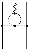
Figure 2: Example of a diagram that leads to an exponentially diverging loop integral when using higher derivative regularization with the ansatz of Eq. (3.9). Solid, dashed and wavy lines refer to nucleons, pions and photons, respectively. Solid dots denote the lowest-order vertices from the effective chiral Lagrangian.

Suppose that both deregularizing factors from the two vertices act on the momentum $l_{1}$. Then, the overall effect of the regulator for the loop contribution is

$$\exp\bigg{(}\frac{l_{1}^{2}+M^{2}}{\Lambda^{2}}\bigg{)}\exp\bigg{(}-\frac{l_{2}^{2}+M^{2}}{\Lambda^{2}}\bigg{)} = \exp\bigg{(}-\frac{2k\cdot l_{1}+k^{2}}{\Lambda^{2}}\bigg{)}.$$ (3.18)

With such an exponential factor, the loop contribution cannot be regularized even using dimensional or $\zeta$-regularization on top of higher-derivative, except for the vanishing photon momentum $k=0$. Thus, the ansatz in Eq. (3.9) still appears to be too restricted for our purposes.

IV Gradient flow regularization

In the last two sections, the higher derivative method was applied to regularize the pion propagator. For both considered modifications of the effective Lagrangian, the failure to simultaneously regularize nuclear forces and currents was caused by deregularization of vertices induced by the additional cutoff-dependent terms. An alternative variant of the higher derivative regularization, which is free from the deregularization issue, is provided by the gradient flow method. During the last decade, the Yang-Mills gradient flow has developed into a powerful tool to address non-perturbative renormalization aspects in the context of lattice QCD, see Refs. Luscher:2011bx ; Luscher:2013cpa ; Luscher:2013vga for pioneering work along this line. The usefulness of this method for lattice QCD applications relies on a smoothing effect for the gauge fields caused by the flow time evolution, which results in an improved or simplified short-distance behavior of correlation functions evaluated at a positive flow time. The idea to use the gradient flow method as a symmetry-preserving regulator in the context of nuclear chiral EFT has been raised in several talks by Kaplan Kaplan . In the considerations below, we follow Ref. Kaplan and show that the resulting regularization scheme fulfills all our requirements and allows one to construct consistently regularized nuclear forces and currents.

Consider the lowest-order Lagrangian for pions given in Eq. (2.2). The corresponding equation of motion is worked out in Appendix B and given in Eq. (3.8). To regularize the pion field, we extend the SU(2) matrix $U(x)$ to $W(x,\tau)$, whose dependence on the parameter $\tau$ is dictated by the chirally covariant version of the gradient flow equation Kaplan

$$\partial_{\tau}W = -iw\,{\rm EOM}(\tau)\,w\,,$$ (4.19)

subject to the boundary condition $W(x,0)=U(x)$. Here, $w(x,\tau)$ is defined through the relationship $W=w^{2}$ and coincides with the matrix $u$ on the boundary, $w(x,0)=u(x)$, while

$${\rm EOM}(\tau) = \big{[}D_{\mu},w_{\mu}\big{]}+\frac{i}{2}\chi_{-}(\tau)-\frac{i}{4}{\rm Tr}\,\chi_{-}(\tau)\,,$$ (4.20)

with

$$\chi_{\pm}(\tau) = w^{\dagger}\chi w^{\dagger}\pm w\chi^{\dagger}w.$$ (4.21)

As one can see from Eqs (4.20) and (4.21), the EOM$(\tau)$ term is constructed out of the EOM defined in Eq. (3.8) by replacing every $u$ field with the $w$ field. The pion-field transformation properties with respect to chiral SU$(2)_{L}\times$SU$(2)_{R}$ rotations are given by

$$U(x) \to R\,U(x)\,L^{\dagger}\,,$$ (4.22)

where $L\in$ SU$(2)_{L}$ and $R\in$ SU$(2)_{R}$. The covariant form of the gradient flow equation (4.19), along with the required boundary condition, guarantees that the field $W(x,\tau)$ has the same transformation properties at any flow “time” $\tau$,

$$W(x,\tau) \to R\,W(x,\tau)\,L^{\dagger}\,,$$ (4.23)

and ensure the unitarity of $W(x,\tau)$. These nontrivial features are proven in Appendix D.

As will be shown below, the solution of the gradient flow equation in terms of the pion fields $\mbox{\boldmath$\pi$}(x)$ introduces a Gaussian smearing in Euclidean space-time, which extends over a distance $\sim\sqrt{2\tau}$. To show this we solve the gradient flow equation (4.19) by performing a $1/F$ expansion of the generalized pion field. The most general parametrization of the unitary matrix $W$ can be written as

$$W = 1+i{\boldsymbol{\tau}}\cdot{\boldsymbol{\phi}}\big{(}1-\alpha\,\mbox{\boldmath$\phi$}^{2}\big{)}-\frac{\mbox{\boldmath$\phi$}^{2}}{2}\bigg{[}1+\bigg{(}\frac{1}{4}-2\alpha\bigg{)}\mbox{\boldmath$\phi$}^{2}\bigg{]}+{\cal O}(\mbox{\boldmath$\phi$}^{5})\,,$$ (4.24)

where $\alpha$ is an arbitrary real constant and the explicit form of the real dimensionless field $\mbox{\boldmath$\phi$}(x,\tau)$ is fixed by the solution of Eq. (4.19). We introduce a metric Meetz:1969as

$$g_{ab} = -\frac{1}{2}{\rm Tr}\bigg{(}W^{\dagger}\frac{\partial W}{\partial\phi_{a}}W^{\dagger}\frac{\partial W}{\partial\phi_{b}}\bigg{)}\,,$$ (4.25)

and multiply both sides of the gradient flow Eq. (4.19) by $W^{\dagger}\partial W/\partial\phi_{a}W^{\dagger}$ from the left. Taking trace we obtain

$$g_{ab}\,\partial_{\tau}\phi_{b} = \frac{i}{2}{\rm Tr}\bigg{[}\frac{\partial W}{\partial\phi_{a}}w^{\dagger}{\rm EOM}(\tau)w^{\dagger}\bigg{]}\,,$$ (4.26)

where we used

$$W^{\dagger}\partial_{\tau}W = W^{\dagger}\frac{\partial W}{\partial\phi_{a}}\partial_{\tau}\phi_{a}\,.$$ (4.27)

Next, we invert Eq. (4.26) to rewrite the gradient flow equation in a form that is more convenient for practical calculations:

$$\partial_{\tau}\phi_{a} = \frac{i}{2}[g^{-1}]_{ab}\,{\rm Tr}\bigg{[}\frac{\partial W}{\partial\phi_{b}}w^{\dagger}{\rm EOM}(\tau)w^{\dagger}\bigg{]}\,.$$ (4.28)

Using the ansatz for $\phi$ in the form of a power series in $1/F$,

$$\phi_{b}=\sum_{n=0}^{\infty}\frac{\phi_{b}^{(n)}}{F^{n}}\,,$$ (4.29)

we obtain a series of recursive differential equations. Restricting ourselves to terms with at most a single insertion of the external sources, the lowest-order equation takes the form

$$\big{[}\partial_{\tau}-(\partial_{\mu}^{x}\partial_{\mu}^{x}-M^{2})\big{]}\phi^{(0)}_{b}(x,\tau) = 2Bp_{b}(x)-\partial_{\mu}a_{\mu b}(x)\,.$$ (4.30)

This linear inhomogeneous differential equation can be solved by introducing the retarded Green’s function, which fulfills

$$\big{[}\partial_{\tau}-(\partial_{\mu}^{x}\partial_{\mu}^{x}-M^{2})\big{]}G(x-y,\tau-s) = \delta(\tau-s)\delta^{4}(x-y)\,,$$ (4.31)

and is given by

$$G(x,\tau) = \theta(\tau)\int\frac{d^{4}q}{(2\pi)^{4}}e^{-\tau(q^{2}+M^{2})}e^{-i\,q\cdot x}\,=\,\frac{\theta(\tau)}{16\pi^{2}\tau^{2}}\,e^{-\frac{x^{2}+4M^{2}\tau^{2}}{4\tau}}\,.$$ (4.32)

Here, $q\cdot x$ denotes an Euclidean product $q\cdot x=q_{0}x_{0}+\vec{q}\cdot\vec{x}$. The solution for $\phi^{(0)}_{b}(x,\tau)$ with the boundary condition $\mbox{\boldmath$\phi$}^{(0)}(x,0)=0$ can be written in terms of the Green’s function via

$$\phi^{(0)}(x,\tau)_{b} = \int_{0}^{\tau}ds\int d^{4}y\,G(x-y,\tau-s)\big{(}2Bp_{b}(y)-\partial_{\mu}a_{\mu b}(y)\big{)}\,.$$ (4.33)

Obviously, the above solution fulfills the desired boundary condition. It is instructive to Fourier transform $\mbox{\boldmath$\phi$}^{(0)}(x,\tau)$ to momentum space:

$$\tilde{\phi}^{(0)}_{b}(q,\tau) = \int d^{4}x\,e^{iq\cdot x}\phi^{(0)}_{b}(x,\tau)\,=\,\int_{0}^{\tau}ds\,e^{-\tau(q^{2}+M^{2})}\big{[}2B\tilde{p}_{b}(q)+iq_{\mu}\tilde{a}_{\mu b}(q)\big{]}\,,$$ (4.34)

where

$$\tilde{p}_{b}(q) = \int d^{4}x\,e^{iq\cdot x}p_{b}(x),\quad\quad\tilde{a}_{\mu b}(q)\,=\,\int d^{4}x\,e^{iq\cdot x}a_{\mu b}(x)\,.$$ (4.35)

Eq. (4.34) can be integrated analytically, leading to

$$\tilde{\phi}^{(0)}_{b}(q,\tau) = \frac{1-e^{-\tau(q^{2}+M^{2})}}{q^{2}+M^{2}}\big{[}2B\tilde{p}_{b}(q)+iq_{\mu}\tilde{a}_{\mu b}(q)\big{]}\,.$$ (4.36)

From Eq. (4.36) we see that $\tilde{\phi}^{(0)}(q,\tau)$ approaches zero linearly with vanishing $\tau$. It is also easy to verify that $\tilde{\phi}^{(0)}(q,\tau)$ satisfies the momentum-space version of the lowest-order gradient flow equation

$$\big{(}\partial_{\tau}+q^{2}+M^{2}\big{)}\tilde{\phi}^{(0)}_{b}(q,\tau) = B\tilde{p}_{b}(q)+iq_{\mu}\tilde{a}_{\mu b}(q)\,,$$ (4.37)

using the trivial identity

$$\big{(}\partial_{\tau}+q^{2}+M^{2}\big{)}\frac{1-e^{-\tau(q^{2}+M^{2})}}{q^{2}+M^{2}} = 1\,.$$ (4.38)

To keep the discussion of higher-order contributions to $\mbox{\boldmath$\phi$}(x,\tau)$ transparent, we switch off all external sources from now on (except for the scalar source, whose value is set to $m_{q}$). Then, the gradient flow equation at order $1/F$ takes a linear homogeneous form

$$\big{[}\partial_{\tau}-(\partial_{\mu}^{x}\partial_{\mu}^{x}-M^{2})\big{]}\phi^{(1)}_{b}(x,\tau) = 0\,,$$ (4.39)

with the boundary condition $\mbox{\boldmath$\phi$}^{(1)}(x,0)=\mbox{\boldmath$\pi$}(x)$, where the pion field $\mbox{\boldmath$\pi$}(x)$ is chosen according to Eq. (3.12). The solution is given by

$$\phi^{(1)}_{b}(x,\tau) = \int d^{4}y\,G(x-y,\tau)\pi_{b}(y)\,,$$ (4.40)

which leads to the momentum-space expression

$$\tilde{\phi}^{(1)}_{b}(q,\tau) = e^{-\tau(q^{2}+M^{2})}\tilde{\pi}_{b}(q)\,.$$ (4.41)

This shows that the gradient flow introduces a Gaussian-type regulator of the pion field.

At order $1/F^{2}$, the gradient flow equation has again a homogeneous form

$$\big{[}\partial_{\tau}-(\partial_{\mu}^{x}\partial_{\mu}^{x}-M^{2})\big{]}\phi^{(2)}_{b}(x,\tau) = 0\,,$$ (4.42)

with the boundary condition $\phi^{(2)}_{b}(x,0)=0$. The only solution that satisfies this condition is a trivial one $\phi^{(2)}_{b}(x,\tau)=0$, so that there are no contributions to $\phi_{b}$ at order $1/F^{2}$ (in the absence of external sources).

At order $1/F^{3}$, we obtain the inhomogeneous linear differential equation for $\mbox{\boldmath$\phi$}^{(3)}(x,\tau)$

$$\big{[}\partial_{\tau}-(\partial_{\mu}^{x}\partial_{\mu}^{x}-M^{2})\big{]}\phi^{(3)}_{b}(x,\tau) = (1-2\alpha)\partial_{\mu}\mbox{\boldmath$\phi$}^{(1)}\cdot\partial_{\mu}\mbox{\boldmath$\phi$}^{(1)}\phi^{(1)}_{b}-4\alpha\,\partial_{\mu}\boldsymbol{\phi}^{(1)}\cdot\boldsymbol{\phi}^{(1)}\partial_{\mu}\phi^{(1)}_{b}$$ (4.43)

$$+ \frac{M^{2}}{2}(1-4\alpha)\boldsymbol{\phi}^{(1)}\cdot\boldsymbol{\phi}^{(1)}\phi^{(1)}_{b}\,.$$

The boundary condition for $\mbox{\boldmath$\phi$}^{(3)}(x,0)$ can be derived by examining the matrix $W(x,\tau)$:

$$W = 1+\frac{i}{F}\boldsymbol{\tau}\cdot\boldsymbol{\phi^{(1)}}-\frac{1}{2F^{2}}\boldsymbol{\phi}^{(1)}\cdot\boldsymbol{\phi}^{(1)}+\frac{i}{F^{3}}\big{(}\boldsymbol{\tau}\cdot\boldsymbol{\phi}^{(3)}-\alpha\,\boldsymbol{\tau}\cdot\boldsymbol{\phi}^{(1)}\boldsymbol{\phi}^{(1)}\cdot\boldsymbol{\phi}^{(1)}\big{)}+\mathcal{O}\bigg{(}\frac{1}{F^{4}}\bigg{)}\,,$$ (4.44)

where we have used that $\mbox{\boldmath$\phi$}^{(2)}(x,\tau)=0$. Given that $\phi_{b}^{(1)}(x,0)=\pi_{b}(x)$, we obtain

$$W\Big{|}_{\tau=0} = 1+\frac{i}{F}\boldsymbol{\tau}\cdot\boldsymbol{\pi}-\frac{1}{2F^{2}}\boldsymbol{\pi}\cdot\boldsymbol{\pi}+\frac{i}{F^{3}}\Big{(}\boldsymbol{\tau}\cdot\boldsymbol{\phi}^{(3)}\Big{|}_{\tau=0}-\alpha\,\boldsymbol{\tau}\cdot\boldsymbol{\pi}\boldsymbol{\pi}\cdot\boldsymbol{\pi}\Big{)}\,.$$ (4.45)

Using $W|_{\tau=0}=U$ and matching Eq. (4.45) to Eq. (3.12), we finally obtain the boundary condition $\mbox{\boldmath$\phi$}^{(3)}(x,0)=0$. We then write the solution of Eq. (4.43) in the form

$$\phi^{(3)}_{b}(x,\tau) = \int_{0}^{\tau}ds\int d^{4}y\,G(x-y,\tau-s)\bigg{[}(1-2\alpha)\partial_{\mu}\mbox{\boldmath$\phi$}^{(1)}(y,s)\cdot\partial_{\mu}\mbox{\boldmath$\phi$}^{(1)}(y,s)\,\phi^{(1)}_{b}(y,s)$$ (4.46)

$$- 4\alpha\,\partial_{\mu}\boldsymbol{\phi}^{(1)}(y,s)\cdot\boldsymbol{\phi}^{(1)}(y,s)\,\partial_{\mu}\phi^{(1)}_{b}(y,s)+\frac{M^{2}}{2}(1-4\alpha)\boldsymbol{\phi}^{(1)}(y,s)\cdot\boldsymbol{\phi}^{(1)}(y,s)\,\phi^{(1)}_{b}(y,s)\bigg{]}\,.$$

The corresponding momentum-space expression is given by

$$\tilde{\phi}^{(3)}_{b}(q,\tau) = \int\frac{d^{4}q_{1}}{(2\pi)^{4}}\frac{d^{4}q_{2}}{(2\pi)^{4}}\frac{d^{4}q_{3}}{(2\pi)^{4}}(2\pi)^{4}\delta^{4}(q-q_{1}-q_{2}-q_{3})\int_{0}^{\tau}ds\,e^{-(\tau-s)(q^{2}+M^{2})}e^{-s\sum_{j=1}^{3}(q_{j}^{2}+M^{2})}$$ (4.47)

$$\times \bigg{[}4\alpha\,q_{1}\cdot q_{3}-(1-2\alpha)q_{1}\cdot q_{2}+\frac{M^{2}}{2}(1-4\alpha)\bigg{]}\tilde{\mbox{\boldmath$\pi$}}(q_{1})\cdot\tilde{\mbox{\boldmath$\pi$}}(q_{2})\,\tilde{\pi}_{b}(q_{3})\,.$$

By looking at the regulator

$$\int_{0}^{\tau}ds\,e^{-(\tau-s)(q^{2}+M^{2})}e^{-s\sum_{j=1}^{3}(q_{j}^{2}+M^{2})} = \frac{e^{-\tau(q^{2}+M^{2})}-e^{-\tau\sum_{j=1}^{3}(q_{j}^{2}+M^{2})}}{q_{1}^{2}+q_{2}^{2}+q_{3}^{2}-q^{2}+2M^{2}}\,,$$ (4.48)

one observes that not every pion field gets regularized since the first Gaussian regulator in the right-hand side of Eq. (4.48) only acts on the total pion momentum $q=q_{1}+q_{2}+q_{3}$. However, as will be argued below, this regularization is sufficient for our purposes. Notice further that the above expression is non-singular for all values of the momenta $q_{i}$ and $q$.

Figure 3: Schematic graphical representation of the solution of the gradient flow equation in coordinate space in the absence of external sources. Red solid dots denote a point in the five-dimensional $(x_{\mu},\tau)$ space, at which the field $\phi$ is evaluated, while black solid dots on the $\tau=0$ boundary correspond to pion locations (being integrated over). Green solid lines refer to the Green’s function defined in Eq. (4.32). Light shaded areas visualize schematically the smearing in Euclidean space-time, whose characteristic size is governed by the gradient flow time.

The above considerations help to elucidate the general structure of the solution of the gradient flow equation $\mbox{\boldmath$\phi$}(x,\tau)$, which is schematically depicted in Fig. 3. Specifically, the field $\mbox{\boldmath$\phi$}(x,\tau)$ is expressed in terms of an increasing number of smeared pion fields that live on the boundary $\tau=0$, with the extent of smearing being controlled by the parameter $\sqrt{2\tau}$. In the limit $\tau\to 0$, all multi-pion contributions to $\phi$ get suppressed and the field $\phi$ turns to the pion field $\pi$.

After these preparations, we are now in the position to define our regularization scheme using the gradient flow method. In the Goldstone boson sector, we employ the standard (i.e., unregularized) Lagrangian $\mathcal{L}_{\pi}=\mathcal{L}_{\pi}^{(2)}+\mathcal{L}_{\pi}^{(4)}+\ldots$, whose lowest-order expression given in Eq. (2.2). The construction of the pionic Lagrangian is conveniently carried out in terms of the matrix $U$, which transforms with respect to chiral rotations according to Eq. (4.22). Different parametrizations of $U$ by the pion fields correspond to different nonlinear realizations of the SU$(2)_{L}\times$SU$(2)_{R}$ group, but lead to the same S-matrix elements. When including matter fields such as nucleons, it is more convenient to employ the SU$(2)$ matrix $u=\sqrt{U}$, see also Eq. (2.1), which possesses somewhat more complicated transformation properties with respect to chiral rotations:

$$u \to R\,u\,K^{\dagger}\,=\,K\,u\,L^{\dagger}\,,$$ (4.49)

where the space-time dependent SU$(2)$ matrix $K(L,R,U)=\sqrt{L\,U^{\dagger}R^{\dagger}}R\,\sqrt{U}$ is referred to as the compensator field. Nucleon fields can then be chosen to transform under chiral rotations according to $N\,\to\,KN$ Coleman:1969sm ; Callan:1969sn . The resulting nonlinear realization of the chiral group allows one to straightforwardly write down the effective chiral Lagrangian in terms of the covariantly transforming building blocks like $u_{\mu}\,\to\,Ku_{\mu}K^{\dagger}$, $D_{\mu}N\,\to\,KD_{\mu}N$, etc., see Eq. (2.1) for the relevant definitions. To construct the regularized pion-nucleon Lagrangian, we follow the same path but use the corresponding building blocks at a nonzero flow time $\tau$, i.e., we replace the pion matrix $U$ by $W(\tau)$ in all expressions in Eq. (2.1) and require the nucleon fields to transform according to $N\,\to\,K(\tau)N$, where $K(\tau)=\sqrt{L\,W^{\dagger}R^{\dagger}}R\,w$ with $w=\sqrt{W}$. The key feature that enables this construction and ensures that the resulting Lagrangian is chirally invariant is the transformation property of the solution of the gradient flow equation, $W(\tau)\to R\,W(\tau)\,L^{\dagger}$, which as shown in Appendix D holds true for all values of the flow parameter $\tau$.

The extension of the Lagrangian to a finite $\tau$, $\mathcal{L}_{\pi N}^{\rm E}\to\mathcal{L}_{\pi N,\tau}^{\rm E}$, leads to new vertices as visualized in Fig. 3 and has a smearing effect on the pion fields that ensures that all pion-nucleon vertices acquire exponential factors, which decrease with growing (combinations of) pion momenta. It is also remarkable that for $\tau\neq 0$, the field $W(\tau)$ does depend, in contrast to the field $U$, on the external sources and has a rather complicated structure. As long as the flow time is kept sufficiently small, i.e. $\tau\sim\Lambda_{b}^{-2}\ll M^{-2}$, where $\Lambda_{b}$ is the breakdown scale of the chiral EFT expansion, the resulting nonlocal effective Lagrangian gives rise to an EFT description of QCD that is equivalent to the standard formulation of chiral perturbation theory (albeit with different values of low-energy constants).

Using the perturbative solution for $\mbox{\boldmath$\phi$}(x,\tau)$ in Eqs. (4.40) and (4.46), along with the expression for the Green’s function in Eq. (4.32), the regularized lowest-order pion-nucleon Lagrangian is found to take the form

$$\mathcal{L}_{\pi N,\tau}^{\rm E\,(1)} = N^{\dagger}\big{(}D_{0}^{w}+gw_{\mu}S_{\mu}\big{)}N\,,$$ (4.50)

with

$$D_{\mu}^{w} = \partial_{\mu}+\Gamma_{\mu}^{w},\quad\Gamma_{\mu}^{w}\,=\,\frac{1}{2}\big{[}w^{\dagger},\partial_{\mu}w\big{]}-\frac{i}{2}w^{\dagger}r_{\mu}w-\frac{i}{2}w\,l_{\mu}w^{\dagger},\quad S_{\mu}=(0,\vec{\sigma}/2)\,.$$ (4.51)

In the absence of external sources, the regularized Lagrangian $\mathcal{L}_{\pi N,\tau}^{\rm E\,(1)}$, expanded in powers of the pion field, takes the form

$${\cal L}_{\pi N,\tau}^{\rm E\,(1)} = N^{\dagger}(x)\bigg{[}-\frac{g}{2F}\vec{\sigma}\cdot\vec{\nabla}_{x}{\cal G}[\delta\mbox{\boldmath$\pi$}](x,\tau)\cdot\mbox{\boldmath$\tau$}+\frac{i}{4F^{2}}\big{(}\mbox{\boldmath$\tau$}\times{\cal G}[\delta\mbox{\boldmath$\pi$}](x,\tau)\big{)}\cdot\partial_{0}^{x}{\cal G}[\delta\mbox{\boldmath$\pi$}](x,\tau)$$ (4.52)

$$+ \frac{g}{4F^{3}}\vec{\sigma}\cdot\vec{\nabla}_{x}\bigg{(}M^{2}(4\alpha-1){\cal G}[\theta{\cal G}[\delta\mbox{\boldmath$\pi$}]\cdot{\cal G}[\delta\mbox{\boldmath$\pi$}]{\cal G}[\delta\mbox{\boldmath$\pi$}]](x,\tau)+2(2\alpha-1){\cal G}[\theta{\cal G}[\delta\partial_{\mu}\mbox{\boldmath$\pi$}]\cdot{\cal G}[\delta\partial_{\mu}\mbox{\boldmath$\pi$}]{\cal G}[\delta\mbox{\boldmath$\pi$}]](x,\tau)$$

$$+ 8\,\alpha\,{\cal G}[\theta{\cal G}[\delta\mbox{\boldmath$\pi$}]\cdot{\cal G}[\delta\partial_{\mu}\mbox{\boldmath$\pi$}]\cdot{\cal G}[\delta\mbox{\boldmath$\pi$}]{\cal G}[\delta\partial_{\mu}\mbox{\boldmath$\pi$}]](x,\tau)+2\,\alpha\,{\cal G}[\delta\mbox{\boldmath$\pi$}](x,\tau)\cdot{\cal G}[\delta\mbox{\boldmath$\pi$}](x,\tau){\cal G}[\delta\mbox{\boldmath$\pi$}](x,\tau)\bigg{)}\cdot\mbox{\boldmath$\tau$}$$

$$- \frac{g}{8F^{3}}\mbox{\boldmath$\tau$}\cdot{\cal G}[\delta\mbox{\boldmath$\pi$}](x,\tau)\vec{\sigma}\cdot\vec{\nabla}_{x}\big{(}{\cal G}[\delta\mbox{\boldmath$\pi$}](x,\tau)\cdot{\cal G}[\delta\mbox{\boldmath$\pi$}](x,\tau)\big{)}\bigg{]}N(x)+{\cal O}(\pi^{4})\,.$$

Here, we have introduced the short-hand notation

$${\cal G}[f](x,\tau) = \int_{-\infty}^{\tau}ds\,e^{-(\tau-s)(-\partial_{x}^{2}+M^{2})}f(x,s),$$ (4.53)

where $f(x,s)$ is a continuous function or distribution. In particular

$${\cal G}[\delta\mbox{\boldmath$\pi$}](x,\tau) = \int_{-\infty}^{\tau}ds\,e^{-(\tau-s)(-\partial_{x}^{2}+M^{2})}\delta(s)\mbox{\boldmath$\pi$}(x)\,=\,e^{-\tau(-\partial_{x}^{2}+M^{2})}\mbox{\boldmath$\pi$}(x)\,,$$ (4.54)

and

$${\cal G}[\theta f](x,\tau) = \int_{-\infty}^{\tau}ds\,e^{-(\tau-s)(-\partial_{x}^{2}+M^{2})}\theta(s)f(x,s)\,=\,\int_{0}^{\tau}ds\,e^{-(\tau-s)(-\partial_{x}^{2}+M^{2})}f(x,s)\,,$$ (4.55)

such that, e.g.,

$${\cal G}[\theta{\cal G}[\delta\mbox{\boldmath$\pi$}]\cdot{\cal G}[\delta\mbox{\boldmath$\pi$}]{\cal G}[\delta\mbox{\boldmath$\pi$}]](x,\tau) = \int_{0}^{\tau}ds\,e^{-(\tau-s)(-\partial_{x}^{2}+M^{2})}{\cal G}[\delta\mbox{\boldmath$\pi$}](x,s)\cdot{\cal G}[\delta\mbox{\boldmath$\pi$}](x,s){\cal G}[\delta\mbox{\boldmath$\pi$}](x,s)$$

$$= \int_{0}^{\tau}ds\,e^{-(\tau-s)(-\partial_{x}^{2}+M^{2})}\bigg{[}e^{-s(-\partial_{x}^{2}+M^{2})}\mbox{\boldmath$\pi$}(x)\bigg{]}\cdot\bigg{[}e^{-s(-\partial_{x}^{2}+M^{2})}\mbox{\boldmath$\pi$}(x)\bigg{]}\bigg{[}e^{-s(-\partial_{x}^{2}+M^{2})}\mbox{\boldmath$\pi$}(x)\bigg{]}\,.$$

When taking the limit $\tau\to 0$, the regularized expression in Eq. (4.52) turns into the unregularized Lagrangian in Eq. (3.13). On the other hand, as already mentioned above, the pionic Lagrangian is not regularized and has the usual form

$$\mathcal{L}_{\pi}^{\rm E\,(2)} = \frac{1}{2}(\partial_{\mu}\mbox{\boldmath$\pi$}\cdot\partial_{\mu}\mbox{\boldmath$\pi$}+M^{2}\mbox{\boldmath$\pi$}^{2})-\frac{1}{F^{2}}\bigg{(}\alpha-\frac{1}{8}\bigg{)}\mbox{\boldmath$\pi$}^{2}\mbox{\boldmath$\pi$}\cdot(-\partial^{2}+M^{2})\mbox{\boldmath$\pi$}-\frac{1}{4F^{2}}\mbox{\boldmath$\pi$}^{2}\partial_{\mu}\mbox{\boldmath$\pi$}\cdot\partial_{\mu}\mbox{\boldmath$\pi$}-\frac{1}{8F^{2}}\mbox{\boldmath$\pi$}^{2}\mbox{\boldmath$\pi$}\cdot\partial^{2}\mbox{\boldmath$\pi$}$$ (4.57)

$$+ \mathcal{O}(\mbox{\boldmath$\pi$}^{6})\,.$$

When using $\mathcal{L}_{\pi N,\tau}^{\rm E\,(1)}$ and $\mathcal{L}_{\pi}^{\rm E\,(2)}$ to derive the one-pion exchange nucleon-nucleon potential, the pion propagator in the static limit acquires the regulator

$$\frac{1}{\vec{q}^{\,2}+M^{2}} \to \frac{e^{-2\tau(\vec{q}^{\,2}+M^{2})}}{\vec{q}^{\,2}+M^{2}}\,.$$ (4.58)

Therefore, to recover the semilocal momentum-space regulator of Refs. Reinert:2017usi ; Reinert:2020mcu we set the flow time to $\tau=1/(2\Lambda^{2})$.

As a proof-of-principle example, we apply the gradient flow method to the 4NF generated by the Feynman diagrams shown in Fig. 1. A straightforward calculation reveals the following result:

$$V^{4N}_{\Lambda} = \frac{g^{4}}{64F^{6}}\mbox{\boldmath$\tau$}_{1}\cdot\mbox{\boldmath$\tau$}_{2}\mbox{\boldmath$\tau$}_{3}\cdot\mbox{\boldmath$\tau$}_{4}\frac{\vec{\sigma}_{2}\cdot\vec{q}_{2}\,\vec{\sigma}_{3}\cdot\vec{q}_{3}\,\vec{\sigma}_{4}\cdot\vec{q}_{4}}{(\vec{q}_{2}^{\,2}+M^{2})(\vec{q}_{3}^{\,2}+M^{2})(\vec{q}_{4}^{\,2}+M^{2})}\bigg{[}\vec{\sigma}_{1}\cdot\vec{q}_{1}\big{(}2g_{\Lambda}-4f_{\Lambda}^{123}+2f_{\Lambda}^{134}-f_{\Lambda}^{234}\big{)}-\vec{\sigma}_{1}\cdot\vec{q}_{2}f_{\Lambda}^{234}$$

$${}\,+2\vec{\sigma}_{1}\cdot\vec{q}_{1}\big{(}5M^{2}+\vec{q}_{1}^{\,2}+\vec{q}_{2}^{\,2}+\vec{q}_{3}^{\,2}+\vec{q}_{4}^{\,2}+\vec{q}_{34}^{\,2}\big{)}\frac{g_{\Lambda}-f_{\Lambda}^{134}}{2M^{2}+\vec{q}_{1}^{\,2}+\vec{q}_{3}^{\,2}+\vec{q}_{4}^{\,2}-\vec{q}_{2}^{\,2}}$$

$${}\,-4\vec{\sigma}_{1}\cdot\vec{q}_{1}\big{(}3M^{2}+\vec{q}_{1}^{\,2}+\vec{q}_{2}^{\,2}+\vec{q}_{3}^{\,2}+\vec{q}_{4}^{\,2}-\vec{q}_{34}^{\,2}\big{)}\frac{g_{\Lambda}-f_{\Lambda}^{124}}{2M^{2}+\vec{q}_{1}^{\,2}+\vec{q}_{2}^{\,2}+\vec{q}_{4}^{\,2}-\vec{q}_{3}^{\,2}}\bigg{]}$$

$$+ \frac{g^{4}}{128F^{6}}\mbox{\boldmath$\tau$}_{1}\cdot\mbox{\boldmath$\tau$}_{2}\mbox{\boldmath$\tau$}_{3}\cdot\mbox{\boldmath$\tau$}_{4}\frac{\vec{\sigma}_{1}\cdot\vec{q}_{1}\,\vec{\sigma}_{2}\cdot\vec{q}_{2}\,\vec{\sigma}_{3}\cdot\vec{q}_{3}\,\vec{\sigma}_{4}\cdot\vec{q}_{4}}{(\vec{q}_{1}^{\,2}+M^{2})(\vec{q}_{2}^{\,2}+M^{2})(\vec{q}_{3}^{\,2}+M^{2})(\vec{q}_{4}^{\,2}+M^{2})}\big{(}M^{2}+\vec{q}_{12}^{\,2}\big{)}\big{(}4f_{\Lambda}^{123}-3g_{\Lambda}\big{)}\,+\,23\text{ perm.},$$

where we have defined

$$g_{\Lambda}\,=\,e^{-\frac{\vec{q}_{1}^{\,2}+M^{2}}{2\Lambda^{2}}}e^{-\frac{\vec{q}_{2}^{\,2}+M^{2}}{2\Lambda^{2}}}e^{-\frac{\vec{q}_{3}^{\,2}+M^{2}}{2\Lambda^{2}}}e^{-\frac{\vec{q}_{4}^{\,2}+M^{2}}{2\Lambda^{2}}}\,.$$ (4.60)

The expression obtained using the gradient flow method differs from the one in Eq. (3.14) calculated using the higher-derivative regularization ansatz of Eq. (3.9), but it also reduces to Eq. (3.16) in the $\Lambda\to\infty$ limit and shows no dependence on the arbitrary parameter $\alpha$, which provides a nontrivial check of our results.

Similarly to the higher-derivative regularization considered in sec. III, the gradient flow method does not eliminate all ultraviolet divergences that appear in loop contributions to the nuclear forces and currents. Some examples of the divergent loop diagrams are shown in Fig. 4.

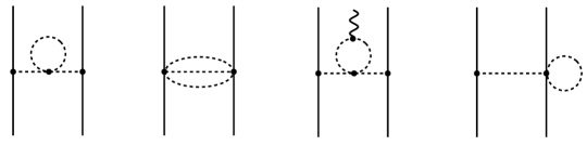
Figure 4: Examples of contributions to the nuclear forces and currents that involve loop integrals, which are not regularized in the gradient flow method. Solid, dashed and wavy lines refer to nucleons, pions and photons, respectively. Solid dots denote the lowest-order vertices from the effective chiral Lagrangian.

However, all such loop contributions involve only pion physics and do not depend on the nucleon propagators. They can, therefore, be safely regularized using an additional dimensional or $\zeta$-function regularization without running into the inconsistency issues mentioned in the introduction. Crucially, all resulting long-range potentials are guaranteed to be sufficiently regularized with respect to the external nucleon momenta, i.e., they can be directly employed in the many-body Schrödinger equation. A distinctive feature of the gradient-flow regularization method is that it does, per construction, not lead to any exponential enhancement in the vertices. For this reason, no issues with exponentially growing integrands that plague the application of the higher-derivative regularization of sec. III to processes involving external sources appear in the gradient-flow method. We thus conclude that this approach fulfills all requirements for a symmetry-preserving regularization scheme formulated in the Introduction.

V Summary and conclusions

In this paper, we have discussed different ways of introducing a cutoff regulator in chiral EFT for nuclear systems. The regulator is required to provide a sufficient suppression of nuclear potentials mediated by single and multiple pion exchanges at large momenta to enable their usage in the many-body Schrödinger equation. In addition, it must respect the chiral and gauge symmetries, and it should ideally reduce to a Gaussian-type cutoff of Refs. Reinert:2017usi ; Reinert:2020mcu when applied to the one-pion exchange two-nucleon potential.

A convenient way to introduce a symmetry-preserving cutoff regulator in an EFT is to appropriately modify the effective Lagrangian by including certain higher-order interactions, as suggested a long time ago by Slavnov in the context of the nonlinear $\sigma$-model Slavnov:1971aw . In our first approach discussed in sec. II, we have considered a simple modification of the lowest-order effective Lagrangian for pions by replacing ${\rm Tr}\big{[}\partial_{\mu}U^{\dagger}\partial_{\mu}U\big{]}\,\to\,{\rm Tr}\Big{[}\partial_{\mu}U^{\dagger}e^{-\partial^{2}/\Lambda^{2}}\partial_{\mu}U\Big{]}$. This modification improves the ultraviolet behavior of the pion propagator, but at the same time introduces new exponentially enhanced vertices with four and more pion fields, which have deregularizing effects. Moreover, since the differential operator in the exponent of the modified Lagrangian acts on several pion fields, the deregularizing factors that appear in the potentials depend on linear combinations of pion momenta and tend to compensate several suppressing factors generated by the regularized pion propagators. In particular, we have shown that the 4NF corresponding to the second diagram of Fig. 1 is not sufficiently regularized using the modified Lagrangian of Eq. (2.3).

The above-mentioned issue can be mitigated if the additional cutoff-dependent terms in the Lagrangian are taken to be proportional to the equation-of-motion terms. Indeed, using the more sophisticated modification of the pion Lagrangian specified in Eq. (3.9) and performing an expansion in powers of the pion fields, all deregularizing exponential operators are found to act on a single pion field, rendering the considered 4NF sufficiently regularized. While the modified Lagrangian of Eq. (3.9) can be applied to derive regularized expressions for long-range nuclear potentials, it still faces its limitations when applied to processes involving external sources. For example, the contribution to the electromagnetic two-nucleon current operator from the diagram shown in Fig. 2 involves an ill-defined loop integral with an exponentially growing integrand (for nonvanishing values of the photon momentum). The considered ansatz is, therefore, still too restricted for our purposes.

The last approach we have considered is the gradient flow method Luscher:2011bx ; Luscher:2013cpa ; Luscher:2013vga . Following Ref. Kaplan , we have introduced a generalized SU(2) matrix $W$ that depends on the artificial flow time $\tau$ and reduces to the ordinary pion matrix $U$ on the $\tau=0$-boundary, $W\stackrel{{\scriptstyle\tau\to 0}}{{\longrightarrow}}U$. The $\tau$-evolution of $W$ is governed by the chirally covariant form of the gradient flow equation (4.19). We have explicitly shown that this equation maintains the transformation properties of the matrix $W$ with respect to chiral rotations, i.e. the relationship $W\to RWL^{\dagger}$ holds true for all values of $\tau$. The matrix $W$ can be expressed in terms of the ordinary pion field $U$ by solving the gradient flow equation, which leads to the appearance of new vertices and Gaussian smearing factors that regularize one or several pion fields. Differently to the previously considered schemes, regularization is achieved by extending the pion-nucleon Lagrangian to a finite flow time $\tau$ while keeping the pionic Lagrangian in its original, unregularized form. This ensures that no problematic exponentially increasing factors emerge (also in the presence of external sources). Moreover, $A$-nucleon connected diagrams acquire exponentially decreasing factors in at least $A-1$ independent combinations of the nucleon momentum transfers $\vec{q}_{i}$, leading to sufficiently regularized nuclear forces and currents. As an explicit example, we worked out the regularized expressions for the 4NF corresponding to the diagrams shown in Fig. 1. The gradient flow method is found to comply with all requirements we impose on the regularization scheme.

In the current paper we have limited ourselves to the application of the regularized effective Lagrangian to the 4NF shown in Fig. 1. These diagrams are of special interest as they involve non-linear pion and pion-nucleon vertices constrained by the chiral symmetry, thereby offering a non-trivial testing ground of the symmetry-preserving nature of the considered regularizations. Since these tree-level diagrams do not involve reducible topologies, the corresponding 4NF can be read off from the scattering amplitude that can be obtained using the Feynman rules. For more general types of diagrams that involve reducible topologies, derivation of nuclear forces and currents requires separating out the irreducible part of the amplitude, which goes beyond the Feynman calculus. In Ref. Krebs:2023ljo , we have formulated a general method to derive nuclear interactions using the path-integral approach, which is capable of treating regularized Lagrangians that involve arbitrarily high number of time derivatives. In subsequent publications, we will apply this method to the gradient-flow-regularized effective Lagrangian to derive consistent nuclear forces and current operators.

Appendix A Derivation of the 4NF in Eq. (2.7) using the path-integral approach of Ref. Krebs:2023ljo

In Ref. Krebs:2023ljo , we have shown how to apply the path-integral approach to the derivation of nuclear potentials. While the 4NF in Eq. (2.7) can be easily obtained by calculating the corresponding Feynman diagram as done in sec. II, here we show how this result can be recapitulated using the path-integral method of Ref. Krebs:2023ljo . Following that work, we consider the lowest-order regularized action for interacting pions and nucleons,

$$S^{\rm E} = \int d^{4}x\,{\cal L}^{\rm E}_{\Lambda},$$ (A.61)

$${\cal L}^{\rm E}_{\Lambda} = N^{\dagger}\bigg{[}\frac{\partial}{\partial x_{0}}\left(1+\frac{1}{\Lambda_{\tau}}\frac{\partial}{\partial x_{0}}\right)-\frac{\vec{\nabla}^{\,2}}{2m}-\frac{g}{2F}\vec{\sigma}\cdot\vec{\nabla}\,\mbox{\boldmath$\pi$}\cdot\mbox{\boldmath$\tau$}\bigg{]}N\,-\,\frac{1}{2}\mbox{\boldmath$\pi$}\cdot\partial^{2}e^{-\partial^{2}/\Lambda^{2}}\mbox{\boldmath$\pi$}\,+\,\frac{1}{8F^{2}}\mbox{\boldmath$\pi$}^{2}\,\partial^{2}e^{-\partial^{2}/\Lambda^{2}}\mbox{\boldmath$\pi$}^{2},$$

where $N$ and $m$ denote the nucleon field and mass, respectively, $\vec{\sigma}$ are the Pauli spin matrices and $g$ refers to the bare axial vector coupling constant in the chiral limit. Further, $\Lambda_{\tau}$ is a temporal cutoff introduced for technical reasons that will be removed at the end of the calculation by taking the limit $\Lambda_{\tau}\to\infty$, see Ref. Krebs:2023ljo for details. The Weinberg-Tomozawa and three-pion-nucleon vertices are not relevant for the illustrative purposes of this example and have been dropped. The action in Eq. (A.61) coincides with the one of the Yukawa model considered in Ref. Krebs:2023ljo except for the vanishing pion mass and the additional four-pion interaction term. Following Ref. Krebs:2023ljo , we proceed with performing the functional integration over pion fields. Since Eq. (2.5) is not quadratic in $\mbox{\boldmath$\pi$}(x)$, we can integrate over the pion field only approximately by using the saddle-point method, i.e. we expand around the minimum of the action. This is equivalent to the loop expansion, which is consistent with the chiral expansion. To find the classical field configuration that minimizes the action $S^{\rm E}$, we take a functional derivative in the pion field and equate it to zero:

$$\frac{\delta S^{\rm E}}{\delta\pi^{j}(x)} = \frac{g}{2F}\vec{\nabla}\cdot\left(N^{\dagger}(x)\vec{\sigma}[\mbox{\boldmath$\tau$}]^{j}N(x)\right)\,-\,\partial^{2}e^{-\partial^{2}/\Lambda^{2}}\pi^{j}(x)\,+\,\frac{1}{2F^{2}}\pi^{j}(x)\,\partial^{2}e^{-\partial^{2}/\Lambda^{2}}\big{(}\mbox{\boldmath$\pi$}(x)\big{)}^{2}\,=\,0.$$ (A.62)

The formal solution of this equation of motion for the pion field is given by

$$\mbox{\boldmath$\pi$}^{c}_{1} = \frac{g}{2F}N_{2}^{\dagger}\mbox{\boldmath$\tau$}\sigma^{i}N_{2}\big{(}\nabla^{i}_{2}\Delta^{\rm E}_{12}\big{)}\,+\,\frac{1}{2F^{2}}\Delta_{12}^{\rm E}\,\mbox{\boldmath$\pi$}^{c}_{2}\,\big{(}\Delta^{\rm E}_{23}\big{)}^{-1}\,\mbox{\boldmath$\pi$}^{c}_{3}\cdot\mbox{\boldmath$\pi$}^{c}_{3}\,+\,{\cal O}(\pi^{5})\,,$$ (A.63)

where $N_{i}\equiv N(x_{i})$, $\mbox{\boldmath$\pi$}_{i}^{c}\equiv\mbox{\boldmath$\pi$}^{c}(x_{i})$, $\vec{\nabla}_{i}\equiv\vec{\nabla}_{x_{i}}$ and the integrations over the coordinates $x_{2}$ and $x_{3}$ are assumed. Further, $\Delta_{ij}^{\rm E}\equiv\Delta^{\rm E}(x_{i}-x_{j})$ denotes the corresponding Green’s function (i.e., the regularized Euclidean pion propagator in the chiral limit as defined in Eq. (2.6)). Replacing the pion field $\pi$ in Eq. (A.62) by the classical solution $\mbox{\boldmath$\pi$}^{c}$, expressed in terms of the nucleon fields, we obtain the nucleonic action in the form

$$S^{\rm E}_{N} = N^{\dagger}_{1}\bigg{[}\partial_{1}^{0}\bigg{(}1+\frac{\partial_{1}^{0}}{\Lambda_{\tau}}\bigg{)}-\frac{\vec{\nabla}^{\,2}}{2m}\bigg{]}N_{1}\,+\,\frac{g^{2}}{8F^{2}}\mbox{\boldmath$\tau$}_{1}\cdot\mbox{\boldmath$\tau$}_{2}\big{(}\vec{\sigma}_{1}\cdot\vec{\nabla}_{1}\vec{\sigma}_{2}\cdot\vec{\nabla}_{1}\Delta^{\rm E}_{12}\big{)}$$

$$- \frac{g^{4}}{128F^{6}}\mbox{\boldmath$\tau$}_{1}\cdot\mbox{\boldmath$\tau$}_{2}\mbox{\boldmath$\tau$}_{3}\cdot\mbox{\boldmath$\tau$}_{4}\big{(}\vec{\sigma}_{1}\cdot\vec{\nabla}_{1}\Delta^{\rm E}_{15}\big{)}\big{(}\vec{\sigma}_{2}\cdot\vec{\nabla}_{2}\Delta^{\rm E}_{25}\big{)}\big{(}\vec{\sigma}_{3}\cdot\vec{\nabla}_{3}\Delta^{\rm E}_{36}\big{)}\big{(}\vec{\sigma}_{4}\cdot\vec{\nabla}_{4}\Delta^{\rm E}_{46}\big{)}\big{(}\Delta^{\rm E}_{56}\big{)}^{-1}\,,$$

where we use the short-hand notation of Ref. Krebs:2023ljo . In particular, we suppress the nucleon fields $N_{i}$ with $i=1,\ldots,4$ (except for the kinetic term) and do not indicate explicitly the integrations over the coordinates $x_{1},\ldots,x_{6}$. The subscript $i$ of the Pauli spin and isospin matrices indicates that they are evaluated between the nucleon fields $N^{\dagger}(x_{i})$ and $N(x_{i})$. This is certainly not the full result since we have neglected Weinberg-Tomozawa and three-pion-nucleon interactions. For this reason, the result in Eq. (A) is only valid in the $\sigma$-model parametrization of the matrix $U$ specified in Eq. (2.4). While one still needs to bring the action $S^{\rm E}_{N}$ into the instantaneous form as described in Ref. Krebs:2023ljo , the contribution to the four-nucleon force we are interested in here can be directly read off from the last term in Eq. (A) by taking the functional derivatives with respect to the nucleon fields. Performing the Fourier transformation to momentum space, the corresponding contribution to the 4N force in the static limit, i.e. for $q_{j}^{0}=0$ with $j=1,\dots,4$, takes the form given in Eq. (2.7).

Appendix B Equation of motion for the pion field

In this appendix we sketch the derivation of the equation of motion for pion fields, following the steps described in Ref. Scherer:2002tk , see also the textbook Meissner:2022cbi . We start with the lowest-order pion Lagrangian in Eq. (2.2) and consider the action

$$S^{(2)} = \int d^{4}x\frac{F^{2}}{4}{\rm Tr}\big{[}\big{(}\nabla_{\mu}U\big{)}^{\dagger}\nabla_{\mu}U-U^{\dagger}\chi-\chi^{\dagger}U\big{]}\,.$$ (B.65)

We perform a variation of the field $U$ by

$$U \to e^{i{\mbox{\boldmath$\epsilon$}}\cdot{\mbox{\boldmath$\tau$}}}U\quad\Rightarrow\quad\delta U\,=\,i{\mbox{\boldmath$\epsilon$}}\cdot{\mbox{\boldmath$\tau$}}U.$$ (B.66)

For the variation of the action $S^{(2)}$, we obtain

$$\delta S^{(2)} = \int d^{4}x\frac{F^{2}}{4}{\rm Tr}\big{[}-\delta U^{\dagger}\nabla_{\mu}\nabla_{\mu}U-(\nabla_{\mu}\nabla_{\mu}U)^{\dagger}\delta U-\delta U^{\dagger}\chi-\chi^{\dagger}\delta U\big{]}$$ (B.67)

$$= \int d^{4}x\frac{F^{2}}{4}{\rm Tr}\big{[}i\,{\mbox{\boldmath$\epsilon$}}\cdot{\mbox{\boldmath$\tau$}}\big{(}(\nabla_{\mu}\nabla_{\mu}U)U^{\dagger}-U(\nabla_{\mu}\nabla_{\mu}U)^{\dagger}+\chi U^{\dagger}-U\chi^{\dagger}\big{)}\big{]}\,.$$

Accordingly, we obtain for the classical equation of motion

$${\rm Tr}\big{[}\tau_{a}\big{(}(\nabla_{\mu}\nabla_{\mu}U)U^{\dagger}-U(\nabla_{\mu}\nabla_{\mu}U)^{\dagger}+\chi U^{\dagger}-U\chi^{\dagger}\big{)}\big{]} = 0\,.$$ (B.68)

We can collect these three equations into a single matrix by noting that any $2\times 2$ matrix $A$ can be written in form

$$A = \mathbb{1}\frac{1}{2}{\rm Tr}A+\frac{1}{2}{\mbox{\boldmath$\tau$}}\cdot{\rm Tr}\big{(}{\mbox{\boldmath$\tau$}}A\big{)}\,.$$ (B.69)

In order for $A=0$ to be equivalent to ${\rm Tr}(\tau_{a}A)=0$, the matrix $A$ has to be traceless. Applying this to the equation of motion (B.68) we obtain

$$(\nabla_{\mu}\nabla_{\mu}U)U^{\dagger}-U(\nabla_{\mu}\nabla_{\mu}U)^{\dagger}+\chi U^{\dagger}-U\chi^{\dagger}\ -\frac{1}{2}{\rm Tr}\big{[}(\nabla_{\mu}\nabla_{\mu}U)U^{\dagger}-U(\nabla_{\mu}\nabla_{\mu}U)^{\dagger}+\chi U^{\dagger}-U\chi^{\dagger}\big{]} = 0,$$ (B.70)

where we made the equation of motion operator traceless by subtracting a half of its trace. Eq. (B.70) can be simplified using the relationship

$${\rm Tr}\big{(}\nabla_{\mu}\nabla_{\mu}UU^{\dagger}\big{)} = {\rm Tr}\big{[}U(\nabla_{\mu}\nabla_{\mu}U)^{\dagger}\big{]}\,.$$ (B.71)

This equality relies on the fact that both $r_{\mu}$ and $l_{\mu}$ are traceless and that $\partial_{\mu}UU^{\dagger}$ is an element of the Lie algebra, i.e. it is traceless. Applying the derivative operator on ${\rm Tr}(\partial_{\mu}UU^{\dagger}-U\partial_{\mu}U^{\dagger})=0$ one gets ${\rm Tr}(\partial_{\mu}\partial_{\mu}UU^{\dagger})={\rm Tr}(U\partial_{\mu}\partial_{\mu}U^{\dagger})$. Rearranging the source terms we obtain Eq. (B.71). Using this relationship Eq. (B.70) simplifies to

$$(\nabla_{\mu}\nabla_{\mu}U)U^{\dagger}-U(\nabla_{\mu}\nabla_{\mu}U)^{\dagger}+\chi U^{\dagger}-U\chi^{\dagger}-\frac{1}{2}{\rm Tr}\big{[}\chi U^{\dagger}-U\chi^{\dagger}\big{]} = 0.$$ (B.72)

To bring the equation of motion to an even more compact form we multiply both sides of Eq. (B.72) with $u$ from the right and with $u^{\dagger}$ from the left as well as with a prefactor $i/2$:

$${\rm EOM}\,=\,\big{[}D_{\mu},u_{\mu}\big{]}+\frac{i}{2}\chi_{-}-\frac{i}{4}{\rm Tr}\chi_{-} = 0\,.$$ (B.73)

Here we used the relationship

$$\frac{i}{2}\big{(}u^{\dagger}(\nabla_{\mu}\nabla_{\mu}U)u^{\dagger}-u(\nabla_{\mu}\nabla_{\mu}U)^{\dagger}u\big{)} = \big{[}D_{\mu},u_{\mu}\big{]}\,.$$ (B.74)

Appendix C Derivation of the regularized Lagrangian in Eq. (III)

In this appendix we expand the regularized Lagrangian of Eq. (3.9) in pion fields $\pi$. We expand the matrix $u_{\mu}$ in powers of the pion field

$$u_{\mu} = -\frac{\mbox{\boldmath$\tau$}\cdot\partial_{\mu}\mbox{\boldmath$\pi$}}{F}-\frac{\mbox{\boldmath$\tau$}\cdot\mbox{\boldmath$\pi$}\mbox{\boldmath$\pi$}\cdot\partial_{\mu}\mbox{\boldmath$\pi$}}{2F^{3}}+\frac{\alpha}{F^{3}}\Big{(}\mbox{\boldmath$\pi$}^{2}\mbox{\boldmath$\tau$}\cdot\partial_{\mu}\mbox{\boldmath$\pi$}+2\mbox{\boldmath$\tau$}\cdot\mbox{\boldmath$\pi$}\mbox{\boldmath$\pi$}\cdot\partial_{\mu}\mbox{\boldmath$\pi$}\Big{)}+{\cal O}(\mbox{\boldmath$\pi$}^{5}),$$ (C.75)

where $\alpha$ is an arbitrary parameter that appears in the parametrization of the ${\rm SU}(2)$ matrix $U$, see Eq. (3.12). In Eq. (C.75) we set all external sources $l_{\mu}$ and $r_{\mu}$ to zero since we focus here on nuclear forces and do not discuss electroweak processes. From Eq. (C.75), we derive the expansion of the ${\rm EOM}$ in powers of the pion field:

$${\rm EOM} = \big{(}-\partial^{2}+M^{2}\big{)}\bigg{[}\frac{\mbox{\boldmath$\tau$}\cdot\mbox{\boldmath$\pi$}}{F}\bigg{(}1-\frac{\alpha}{F^{2}}\mbox{\boldmath$\pi$}^{2}\bigg{)}\bigg{]}-\frac{\mbox{\boldmath$\tau$}\cdot\mbox{\boldmath$\pi$}}{F^{3}}\bigg{(}\partial_{\mu}\mbox{\boldmath$\pi$}\cdot\partial_{\mu}\mbox{\boldmath$\pi$}+\frac{1}{2}\mbox{\boldmath$\pi$}\cdot\partial^{2}\mbox{\boldmath$\pi$}\bigg{)}+{\cal O}(\mbox{\boldmath$\pi$}^{5}).\quad$$ (C.76)

To expand Eq. (3.9) in powers of $\pi$, we first need to obtain an expansion of the exponential operator, which depends on the covariant derivatives. To do this we introduce a modified covariant derivative

$$D_{\mu}^{\lambda} = \partial_{\mu}+\lambda\Gamma_{\mu},$$ (C.77)

where $\lambda$ is an arbitrary parameter. For $\lambda=0$, the connection $\Gamma_{\mu}$ is switched off while for $\lambda=1$, the covariant derivative acquires its original form. In a similar way, we introduce

$$\chi_{+}^{\lambda} = 2M^{2}+\lambda\left(\chi_{+}-2M^{2}\right).$$ (C.78)

Furthermore, we use the expressions

$$\Gamma_{\mu} = \frac{i}{4F^{2}}\mbox{\boldmath$\tau$}\cdot(\mbox{\boldmath$\pi$}\times\partial_{\mu}\mbox{\boldmath$\pi$})+\frac{i}{16F^{4}}\mbox{\boldmath$\pi$}^{2}\mbox{\boldmath$\tau$}\cdot(\mbox{\boldmath$\pi$}\times\partial_{\mu}\mbox{\boldmath$\pi$})-\frac{i\,\alpha}{2F^{4}}\mbox{\boldmath$\pi$}^{2}\mbox{\boldmath$\tau$}\cdot(\mbox{\boldmath$\pi$}\times\partial_{\mu}\mbox{\boldmath$\pi$})+{\cal O}(\mbox{\boldmath$\pi$}^{6}),$$

$$\chi_{+} = 2M^{2}-\frac{M^{2}}{F^{2}}\mbox{\boldmath$\pi$}^{2}-\frac{(1-8\alpha)M^{2}}{4F^{4}}\mbox{\boldmath$\pi$}^{4}+{\cal O}(\mbox{\boldmath$\pi$}^{6})\,,$$ (C.79)

where we have switched off all electroweak and pseudoscalar external sources and set the scalar source to the light quark mass $m_{q}$. Isospin-breaking corrections to $\chi_{+}$ are neglected. The exponential operator in Eq. (3.9) can be expressed in the form

$$\exp\left(\frac{-{\rm ad}_{D_{\mu}}{\rm ad}_{D_{\mu}}+\frac{1}{2}\chi_{+}}{\Lambda^{2}}\right) = \exp\left(\frac{-{\rm ad}_{\partial_{\mu}}{\rm ad}_{\partial_{\mu}}+M^{2}}{\Lambda^{2}}\right)\bigg{[}1+\int_{0}^{1}ds\,\exp\bigg{(}-s\frac{-{\rm ad}_{\partial_{\mu}}{\rm ad}_{\partial_{\mu}}+M^{2}}{\Lambda^{2}}\bigg{)}$$ (C.80)

$$\times \frac{-\left\{{\rm ad}_{\partial_{\mu}},{\rm ad}_{\Gamma_{\mu}}\right\}+\frac{1}{2}\big{(}\chi_{+}-2M^{2}\big{)}}{\Lambda^{2}}\exp\bigg{(}s\frac{-{\rm ad}_{\partial_{\mu}}{\rm ad}_{\partial_{\mu}}+M^{2}}{\Lambda^{2}}\bigg{)}\bigg{]}+{\cal O}(\mbox{\boldmath$\pi$}^{4}).$$

The identity in Eq. (C.80) is easily proven by using time-dependent perturbation theory. For the sake of compactness, we introduce

$$B = \frac{-{\rm ad}_{D_{\mu}}{\rm ad}_{D_{\mu}}+\frac{1}{2}\chi_{+}}{\Lambda^{2}},\quad\quad B_{0}\,=\,\frac{-{\rm ad}_{\partial_{\mu}}{\rm ad}_{\partial_{\mu}}+M^{2}}{\Lambda^{2}},\quad\quad\delta B\,=\,B-B_{0}\,=\,\frac{-\left\{{\rm ad}_{\partial_{\mu}},{\rm ad}_{\Gamma_{\mu}}\right\}+\frac{1}{2}\big{(}\chi_{+}-2M^{2}\big{)}}{\Lambda^{2}}.$$

We recall the well-known result of time-dependent perturbation theory

$$\exp(B) = \exp(B_{0})T\exp\bigg{(}\int_{0}^{1}ds\,\delta B_{I}(s)\bigg{)},$$ (C.81)

where the perturbation in the interaction picture is given by

$$\delta B_{I}(s) = \exp(-sB_{0})\delta B\exp(sB_{0}).$$ (C.82)

Expanding the operator

$$T\exp\bigg{(}\int_{0}^{1}ds\,\delta B_{I}(s)\bigg{)} = 1+\sum_{n=1}^{\infty}\int_{0}^{1}ds_{1}\int_{0}^{s_{1}}ds_{2}\dots\int_{0}^{s_{n-1}}ds_{n}\delta B_{I}(s_{1})\delta B_{I}(s_{2})\dots\delta B_{I}(s_{n}),$$ (C.83)

up to first order in $\delta B_{I}(s)$ yields Eq. (C.80). Notice that we do not employ the large-cutoff expansion since $\Lambda$ is going to be kept fixed throughout the calculation. The only expansion we make use of is the chiral expansion in powers of $1/(4\pi F)$. Using Eq. (C.80), we obtain the expression for the operator appearing in the Lagrangian in the form

$$\frac{1-\exp\left(\frac{-{\rm ad}_{D_{\mu}}{\rm ad}_{D_{\mu}}+\frac{1}{2}\chi_{+}}{\Lambda^{2}}\right)}{-{\rm ad}_{D_{\mu}}{\rm ad}_{D_{\mu}}+\frac{1}{2}\chi_{+}} = \frac{1-\exp\Big{(}\frac{-{\rm ad}_{\partial_{\mu}}{\rm ad}_{\partial_{\mu}}+M^{2}}{\Lambda^{2}}\Big{)}}{-{\rm ad}_{\partial_{\mu}}{\rm ad}_{\partial_{\mu}}+M^{2}}+K_{1}+K_{2}+{\cal O}(\mbox{\boldmath$\pi$}^{3}),$$ (C.84)

where the operators $K_{1,2}$ are defined by

$$K_{1} = -\frac{1}{-{\rm ad}_{\partial_{\mu}}{\rm ad}_{\partial_{\mu}}+M^{2}}\Big{[}-\big{\{}{\rm ad}_{\partial_{\mu}},{\rm ad}_{\Gamma_{\mu}}\big{\}}+\frac{1}{2}\big{(}\chi_{+}-2M^{2}\big{)}\Big{]}\frac{1}{-{\rm ad}_{\partial_{\mu}}{\rm ad}_{\partial_{\mu}}+M^{2}}\bigg{[}1-\exp\bigg{(}\frac{-{\rm ad}_{\partial_{\mu}}{\rm ad}_{\partial_{\mu}}+M^{2}}{\Lambda^{2}}\bigg{)}\bigg{]},$$

$$K_{2} = -\frac{1}{-{\rm ad}_{\partial_{\mu}}{\rm ad}_{\partial_{\mu}}+M^{2}}\int_{0}^{1}ds\exp\bigg{[}(1-s)\frac{-{\rm ad}_{\partial_{\mu}}{\rm ad}_{\partial_{\mu}}+M^{2}}{\Lambda^{2}}\bigg{]}\frac{-\big{\{}{\rm ad}_{\partial_{\mu}},{\rm ad}_{\Gamma_{\mu}}\big{\}}+\frac{1}{2}\big{(}\chi_{+}-2M^{2}\big{)}}{\Lambda^{2}}$$ (C.85)

$$\times \exp\bigg{(}s\frac{-{\rm ad}_{\partial_{\mu}}{\rm ad}_{\partial_{\mu}}+M^{2}}{\Lambda^{2}}\bigg{)}.$$

Here, we used the standard relation

$$\frac{1}{A+B}-\frac{1}{A} = -\frac{1}{A}B\frac{1}{A}+{\cal O}(B^{2}),$$ (C.86)

valid for operators $A$ and $B$. We can rewrite $K_{1}$ into

$$K_{1} = \frac{1}{-{\rm ad}_{\partial_{\mu}}{\rm ad}_{\partial_{\mu}}+M^{2}}\frac{-\big{\{}{\rm ad}_{\partial_{\mu}},{\rm ad}_{\Gamma_{\mu}}\big{\}}+\frac{1}{2}\big{(}\chi_{+}-2M^{2}\big{)}}{\Lambda^{2}}\int_{0}^{1}ds\exp\bigg{(}s\frac{-{\rm ad}_{\partial_{\mu}}{\rm ad}_{\partial_{\mu}}+M^{2}}{\Lambda^{2}}\bigg{)},$$ (C.87)

such that

$$K_{1}+K_{2} = \frac{1}{-{\rm ad}_{\partial_{\mu}}{\rm ad}_{\partial_{\mu}}+M^{2}}\int_{0}^{1}ds\left[1-\exp\bigg{(}(1-s)\frac{-{\rm ad}_{\partial_{\mu}}{\rm ad}_{\partial_{\mu}}+M^{2}}{\Lambda^{2}}\bigg{)}\right]\frac{-\frac{i}{2}\,\big{\{}{\rm ad}_{\partial_{\mu}},{\rm ad}_{\mbox{\boldmath$\tau$}\cdot\big{(}\mbox{\boldmath$\pi$}\times\partial_{\mu}\mbox{\boldmath$\pi$}\big{)}}\big{\}}-M^{2}\mbox{\boldmath$\pi$}^{2}}{2F^{2}\Lambda^{2}}$$ (C.88)

$$\times \exp\bigg{(}s\frac{-{\rm ad}_{\partial_{\mu}}{\rm ad}_{\partial_{\mu}}+M^{2}}{\Lambda^{2}}\bigg{)}+{\cal O}(\mbox{\boldmath$\pi$}^{4}).$$

Further, keeping the terms with up to four pion fields, we obtain

$$-\frac{F^{2}}{4}{\rm Tr}\,{\rm EOM}\frac{1}{-{\rm ad}_{\partial_{\mu}}{\rm ad}_{\partial_{\mu}}+M^{2}}{\rm EOM} = -\frac{1}{2}\mbox{\boldmath$\pi$}\cdot\big{(}-\partial^{2}+M^{2}\big{)}\mbox{\boldmath$\pi$}+\frac{\alpha}{F^{2}}\mbox{\boldmath$\pi$}^{2}\mbox{\boldmath$\pi$}\cdot\big{(}-\partial^{2}+M^{2}\big{)}\mbox{\boldmath$\pi$}$$ (C.89)

$$+ \frac{\mbox{\boldmath$\pi$}^{2}}{F^{2}}\bigg{(}\partial_{\mu}\mbox{\boldmath$\pi$}\cdot\partial_{\mu}\mbox{\boldmath$\pi$}+\frac{1}{2}\mbox{\boldmath$\pi$}\cdot\partial^{2}\mbox{\boldmath$\pi$}\bigg{)}+{\cal O}(\mbox{\boldmath$\pi$}^{6}).$$

For the unregularized pion Lagrangian in Eq. (3.9), we have

$${\cal L}_{\pi}^{\rm E\,(2)} = -F^{2}M^{2}-\frac{1}{2}\mbox{\boldmath$\pi$}\cdot\big{(}\partial^{2}-M^{2}\big{)}\mbox{\boldmath$\pi$}+\frac{\mbox{\boldmath$\pi$}^{2}}{8F^{2}}\Big{[}-2\partial_{\mu}\mbox{\boldmath$\pi$}\cdot\partial_{\mu}\mbox{\boldmath$\pi$}-\mbox{\boldmath$\pi$}\cdot\partial^{2}\mbox{\boldmath$\pi$}+(1-8\alpha)\mbox{\boldmath$\pi$}\cdot(-\partial^{2}+M^{2})\mbox{\boldmath$\pi$}\Big{]}+{\cal O}(\mbox{\boldmath$\pi$}^{6}).\quad\quad$$ (C.90)

Combining Eqs. (C.89) and (C.90), we end up with

$${\cal L}_{\pi}^{\rm E\,(2)}-\frac{F^{2}}{4}{\rm Tr}\,{\rm EOM}\frac{1}{-{\rm ad}_{\partial_{\mu}}{\rm ad}_{\partial_{\mu}}+M^{2}}{\rm EOM} = -F^{2}M^{2}+\frac{\mbox{\boldmath$\pi$}^{2}}{8F^{2}}\Big{[}6\,\partial_{\mu}\mbox{\boldmath$\pi$}\cdot\partial_{\mu}\mbox{\boldmath$\pi$}+3\,\mbox{\boldmath$\pi$}\cdot\partial^{2}\mbox{\boldmath$\pi$}+\mbox{\boldmath$\pi$}\cdot(-\partial^{2}+M^{2})\mbox{\boldmath$\pi$}\Big{]}$$ (C.91)

$$+ {\cal O}(\mbox{\boldmath$\pi$}^{6}).\quad$$

The exponential operator with the propagator sandwiched between the EOM terms is given by

$$\frac{F^{2}}{4}{\rm Tr}\,{\rm EOM}\frac{\exp\Big{(}\frac{-{\rm ad}_{\partial_{\mu}}{\rm ad}_{\partial_{\mu}}+M^{2}}{\Lambda^{2}}\Big{)}}{-{\rm ad}_{\partial_{\mu}}{\rm ad}_{\partial_{\mu}}+M^{2}}{\rm EOM} = \frac{1}{2}\mbox{\boldmath$\pi$}\cdot\big{(}-\partial^{2}+M^{2}\big{)}e^{\frac{-\partial^{2}+M^{2}}{\Lambda^{2}}}\mbox{\boldmath$\pi$}-\frac{\alpha}{F^{2}}\mbox{\boldmath$\pi$}^{2}\mbox{\boldmath$\pi$}\cdot\big{(}-\partial^{2}+M^{2}\big{)}e^{\frac{-\partial^{2}+M^{2}}{\Lambda^{2}}}\mbox{\boldmath$\pi$}$$ (C.92)

$$- \frac{1}{F^{2}}\bigg{(}\partial_{\mu}\mbox{\boldmath$\pi$}\cdot\partial_{\mu}\mbox{\boldmath$\pi$}+\frac{1}{2}\mbox{\boldmath$\pi$}\cdot\partial^{2}\mbox{\boldmath$\pi$}\bigg{)}\mbox{\boldmath$\pi$}\cdot e^{\frac{-\partial^{2}+M^{2}}{\Lambda^{2}}}\mbox{\boldmath$\pi$}+{\cal O}(\mbox{\boldmath$\pi$}^{6}).$$

Using Eq. (C.88), we obtain

$$-\frac{F^{2}}{4}{\rm Tr}\,{\rm EOM}\big{(}K_{1}+K_{2}\big{)}{\rm EOM} = \frac{1}{4F^{2}\Lambda^{2}}\int_{0}^{1}ds\bigg{\{}M^{2}\mbox{\boldmath$\pi$}^{2}\bigg{[}\bigg{(}1-e^{(1-s)\frac{-\partial^{2}+M^{2}}{\Lambda^{2}}}\bigg{)}\mbox{\boldmath$\pi$}\bigg{]}\cdot\bigg{[}\big{(}-\partial^{2}+M^{2}\big{)}e^{s\frac{-\partial^{2}+M^{2}}{\Lambda^{2}}}\mbox{\boldmath$\pi$}\bigg{]}$$ (C.93)

$$+ \big{(}\mbox{\boldmath$\pi$}\times\partial_{\mu}\mbox{\boldmath$\pi$}\big{)}\cdot\bigg{[}\bigg{(}e^{s\frac{-\partial^{2}+M^{2}}{\Lambda^{2}}}\big{(}-\partial^{2}+M^{2}\big{)}\mbox{\boldmath$\pi$}\bigg{)}\times\overleftrightarrow{\partial}_{\!\!\mu}\bigg{(}1-^{(1-s)\frac{-\partial^{2}+M^{2}}{\Lambda^{2}}}\bigg{)}\mbox{\boldmath$\pi$}\bigg{]}\bigg{\}}$$

$$+ {\cal O}(\mbox{\boldmath$\pi$}^{6}),$$

where we have used the notation

$$A\cdot\Big{[}B\times\overleftrightarrow{\partial}_{\!\!\mu}C\Big{]} = A\cdot\Big{[}B\times\partial_{\mu}C\Big{]}-A\cdot\Big{[}\big{(}\partial_{\mu}B\big{)}\times C\Big{]}.$$ (C.94)

The double-cross product in Eq. (C.93) is generated by the connection $\Gamma_{\mu}$. Combining the terms in Eqs. (C.91), (C.92) and (C.93), we finally arrive at the regularized Lagrangian ${\cal L}_{\pi,\Lambda}^{\rm E\,(2)}$ given in Eq. (III).

Appendix D Gradient flow in chiral perturbation theory

Here, we give a proof that the solution $W$ of the gradient flow equation (4.19) is an element of $SU(2)$ and transforms linearly under chiral transformations, i.e.  $W\to R\,W\,L^{\dagger}$.

To show that $W$ is unitary, we consider the gradient flow equation written in the form

$$\partial_{\tau}WW^{\dagger} = -\frac{i}{2}w\big{(}{\rm EOM}(\tau)+{\rm EOM}^{\dagger}(\tau)\big{)}w^{\dagger}\,.$$ (D.95)

Equation (D.95) is identical to Eq. (4.19) if the matrix $W$ is unitary. If we take Eq. (D.95) as a definition of the gradient flow equation, then the unitarity of $W$ follows immediately by taking hermitian conjugate of this equation, yielding

$$W\partial_{\tau}W^{\dagger} = \frac{i}{2}w\big{(}{\rm EOM}(\tau)+{\rm EOM}^{\dagger}(\tau)\big{)}w^{\dagger}\,.$$ (D.96)

Adding Eqs. (D.95) and (D.96), we obtain

$$\partial_{\tau}\big{(}W\,W^{\dagger}\big{)}=\partial W\,W^{\dagger}+W\partial_{\tau}W^{\dagger} = 0\quad\Rightarrow\quad W\,W^{\dagger}\,=\,{\rm const}\,.$$ (D.97)

To show that $\det W=1$, we use the Jacobi formula for a derivative of a determinant:

$$\partial_{\tau}\det W = \det W\,{\rm Tr}\big{(}W^{-1}\partial_{\tau}W\big{)}\,.$$ (D.98)

Exploiting the unitarity of $W$ and using the gradient flow Eq. (D.96), we obtain from Eq. (D.98)

$$\partial_{\tau}\det W = -\frac{i}{2}\det W\,{\rm Tr}\Big{[}W^{\dagger}w\big{(}{\rm EOM}(\tau)+{\rm EOM}^{\dagger}(\tau)\big{)}w\Big{]}$$ (D.99)

$$= -\frac{i}{2}\det W\,{\rm Tr}\big{[}{\rm EOM}(\tau)+{\rm EOM}^{\dagger}(\tau)\big{]}\,=\,0\,,$$

where in the last step of Eq. (D.99) we used that the ${\rm EOM}(\tau)$ operator is traceless (by construction). Since $\det W$ does not depend on $\tau$ and $\det W(\tau=0)=\det U=1$, it follows that $\det W=1$. This implies that $W$ is an element of the SU$(2)$ group for all values of $\tau$.

To prove the chiral transformation properties of $W$, we rewrite the EOM$(\tau)$ operator via

$$-i\,w\,{\rm EOM}(\tau)\,w = \frac{1}{2}\bigg{[}(\nabla_{\mu}\nabla_{\mu}W)W^{\dagger}-W(\nabla_{\mu}\nabla_{\mu}W)^{\dagger}+\chi W^{\dagger}-W\chi^{\dagger}-\frac{1}{2}{\rm Tr}\big{(}\chi W^{\dagger}-W\chi^{\dagger}\big{)}\bigg{]}\,W\,.$$ (D.100)

Here, we used the definition of the EOM in Eqs. (B.72) and (B.73). Thus, the gradient flow equation (4.19) is rewritten to

$$\partial_{\tau}W = \frac{1}{2}\bigg{[}(\nabla_{\mu}\nabla_{\mu}W)W^{\dagger}-W(\nabla_{\mu}\nabla_{\mu}W)^{\dagger}+\chi W^{\dagger}-W\chi^{\dagger}-\frac{1}{2}{\rm Tr}\big{(}\chi W^{\dagger}-W\chi^{\dagger}\big{)}\bigg{]}\,W\,.$$ (D.101)

Equation (D.101) is more convenient for studying the chiral transformation properties, since everything here is expressed in terms of $W$. Next, we perform the small-$\tau$ expansion

$$W = \sum_{n=0}^{\infty}\tau^{n}W^{(n)}\,,$$ (D.102)

where $W^{(n)}$ does not depend on $\tau$. Eq. (D.101) then becomes

$$\sum_{n=0}^{\infty}(n+1)\tau^{n}W^{(n+1)} = \frac{1}{2}\chi+\sum_{n=0}^{\infty}\tau^{n}\frac{1}{2}\bigg{[}\nabla_{\mu}\nabla_{\mu}W^{(n)}-\sum_{n_{1}+n_{2}+n_{3}=n}W^{(n_{1})}(\nabla_{\mu}\nabla_{\mu}W^{(n_{2})})^{\dagger}W^{(n_{3})}$$ (D.103)

$$- \sum_{n_{1}+n_{2}=n}\bigg{(}W^{(n_{1})}\chi^{\dagger}W^{(n_{2})}+\frac{1}{2}{\rm Tr}\big{[}\chi W^{(n_{1})\dagger}-W^{(n_{1})}\chi^{\dagger}\big{]}W^{(n_{2})}\bigg{)}\bigg{]}\,.$$

Eq. (D.103) provides a recursion relation, which allows one to verify the transformation properties of the $W^{(n)}$ operators. We start the induction with $n=0$ and obtain

$$W^{(1)} = \frac{1}{2}\chi+\frac{1}{2}\bigg{[}\nabla_{\mu}\nabla_{\mu}W^{(0)}-W^{(0)}(\nabla_{\mu}\nabla_{\mu}W^{(0)})^{\dagger}W^{(0)}-W^{(0)}\chi^{\dagger}W^{(0)}-\frac{1}{2}{\rm Tr}\big{(}\chi W^{(0)\dagger}-W^{(0)}\chi^{\dagger}\big{)}W^{(0)}\bigg{]}$$ (D.104)

$$= \frac{1}{2}\chi+\frac{1}{2}\bigg{[}\nabla_{\mu}\nabla_{\mu}U-U(\nabla_{\mu}\nabla_{\mu}U)^{\dagger}U-U\chi^{\dagger}U-\frac{1}{2}{\rm Tr}\big{[}\chi U^{\dagger}-U\chi^{\dagger}\big{]}U\bigg{]}\,.$$

Under chiral rotations, the field $U$, its covariant derivative and the source $\chi$ transform via

$$\chi \to R\,\chi\,L^{\dagger},\quad\quad U\,\to\,R\,U\,L^{\dagger},\quad\quad\nabla_{\mu}U\,\to\,R\,\nabla_{\mu}UL^{\dagger}\,.$$ (D.105)

Thus, we see that $W^{(1)}$ transforms as

$$W^{(1)} \to R\,W^{(1)}\,L^{\dagger}\,.$$ (D.106)

Notice that covariant derivatives $\nabla_{\mu}$ do not depend on $W$:

$$\nabla_{\mu}W^{(1)}=\partial_{\mu}W^{(1)}-i\,r_{\mu}W^{(1)}+i\,W^{(1)}l_{\mu}.$$ (D.107)

Since $W^{(1)}$ has the same behaviour under chiral transformations as $U$, the covariant derivative of $W^{(1)}$ transforms as

$$\nabla_{\mu}W^{(1)} \to R\,\nabla_{\mu}W^{(1)}\,L^{\dagger}\,.$$ (D.108)

Suppose now that $W^{(j)}$ transforms as

$$W^{(j)} \to R\,W^{(j)}\,L^{\dagger}\,,$$ (D.109)

for $j\leq n$. Then, Eq. (D.103) fixes the transformation behaviour of $W^{(n+1)}$:

$$W^{(n+1)} = \frac{1}{n+1}\bigg{[}\frac{1}{2}\nabla_{\mu}\nabla_{\mu}W^{(n)}-\sum_{n_{1}+n_{2}+n_{3}=n}W^{(n_{1})}(\nabla_{\mu}\nabla_{\mu}W^{(n_{2})})^{\dagger}W^{(n_{3})}$$ (D.110)

$$- \sum_{n_{1}+n_{2}=n}\bigg{(}W^{(n_{1})}\chi^{\dagger}W^{(n_{2})}+\frac{1}{2}{\rm Tr}\big{[}\chi W^{(n_{1})\dagger}-W^{(n_{1})}\chi^{\dagger}\big{]}W^{(n_{2})}\bigg{)}\bigg{]}\,.$$

Since on the right-hand side of Eq. (D.110) all superscripts of $W$ are smaller or equal $n$, we conclude that

$$W^{(n+1)} \to R\,W^{(n+1)}\,L^{\dagger}.$$ (D.111)

This proves the desired relationship

$$W \to R\,W\,L^{\dagger}.$$ (D.112)

References

- (1) E. Epelbaum, H. W.-Hammer and U.-G. Meißner, Rev. Mod. Phys. 81, 1773-1825 (2009) [arXiv:0811.1338 [nucl-th]].
- (2) R. Machleidt and D. R. Entem, Phys. Rept. 503, 1-75 (2011) [arXiv:1105.2919 [nucl-th]].
- (3) A. M. Gasparyan and E. Epelbaum, Phys. Rev. C 105, no.2, 024001 (2022) [arXiv:2110.15302 [nucl-th]].
- (4) A. M. Gasparyan and E. Epelbaum, Phys. Rev. C 107, no.4, 044002 (2023) [arXiv:2301.13032 [nucl-th]].
- (5) E. Epelbaum, H. Krebs and P. Reinert, Front. in Phys. 8, 98 (2020) [arXiv:1911.11875 [nucl-th]].
- (6) H. Krebs, PoS CD2018, 098 (2019) [arXiv:1908.01538 [nucl-th]].
- (7) P. Reinert, H. Krebs and E. Epelbaum, Eur. Phys. J. A 54, no.5, 86 (2018) [arXiv:1711.08821 [nucl-th]].
- (8) H. Krebs and E. Epelbaum, [arXiv:2311.10893 [nucl-th]].
- (9) A. A. Slavnov, Nucl. Phys. B 31, 301-315 (1971)
- (10) D. Djukanovic, M. R. Schindler, J. Gegelia and S. Scherer, Phys. Rev. D 72, 045002 (2005) [arXiv:hep-ph/0407170 [hep-ph]].
- (11) B. Long and Y. Mei, Phys. Rev. C 93, no.4, 044003 (2016) [arXiv:1605.02153 [nucl-th]].
- (12) D. Kaplan, Gradient flow for chiral effective theories, talk at the Workshop on Hadrons and Hadron Interactions in QCD (HHIQCD 2015), February 15 - March 21, 2015, Yukawa Institute for Theoretical Physics, Kyoto University, Japan; Gradient flow for chiral interactions, seminar talk on April 19, 2016 at INT, Seattle, USA.
- (13) V. Bernard, N. Kaiser and U.-G. Meißner, Int. J. Mod. Phys. E 4, 193-346 (1995) [arXiv:hep-ph/9501384 [hep-ph]].
- (14) H. Krebs, E. Epelbaum and U.-G. Meißner, Eur. Phys. J. A 56, no.9, 240 (2020) [arXiv:2005.07433 [nucl-th]].
- (15) E. Epelbaum, H. Krebs and P. Reinert, [arXiv:2206.07072 [nucl-th]].
- (16) P. Reinert, H. Krebs and E. Epelbaum, Phys. Rev. Lett. 126, no.9, 092501 (2021) [arXiv:2006.15360 [nucl-th]].
- (17) E. Epelbaum, W. Glöckle and U.-G. Meißner, Nucl. Phys. A 637, 107-134 (1998) [arXiv:nucl-th/9801064 [nucl-th]].
- (18) E. Epelbaum, Phys. Lett. B 639, 456-461 (2006) [arXiv:nucl-th/0511025 [nucl-th]].
- (19) E. Epelbaum, Eur. Phys. J. A 34, 197-214 (2007) [arXiv:0710.4250 [nucl-th]].
- (20) M. Lüscher and P. Weisz, JHEP 02, 051 (2011) [arXiv:1101.0963 [hep-th]].
- (21) M. Lüscher, JHEP 04 (2013), 123 [arXiv:1302.5246 [hep-lat]].
- (22) M. Lüscher, PoS LATTICE2013, 016 (2014) [arXiv:1308.5598 [hep-lat]].
- (23) K. Meetz, J. Math. Phys. 10 (1969), 589-593
- (24) S. R. Coleman, J. Wess and B. Zumino, Phys. Rev. 177, 2239-2247 (1969)
- (25) C. G. Callan, Jr., S. R. Coleman, J. Wess and B. Zumino, Phys. Rev. 177, 2247-2250 (1969)
- (26) S. Scherer, Adv. Nucl. Phys. 27 (2003), 277 [arXiv:hep-ph/0210398 [hep-ph]].
- (27) U.-G. Meißner and A. Rusetsky, Effective Field Theories, ISBN 978-1-108-68903-8, Cambridge University Press, 2022,