On the convergence of loss and uncertainty-based active learning algorithms

Abstract

We study convergence rates of loss and uncertainty-based active learning algorithms under various assumptions. First, we provide a set of conditions under which a convergence rate guarantee holds, and use this for linear classifiers and linearly separable datasets to show convergence rate guarantees for loss-based sampling and different loss functions. Second, we provide a framework that allows us to derive convergence rate bounds for loss-based sampling by deploying known convergence rate bounds for stochastic gradient descent algorithms. Third, and last, we propose an active learning algorithm that combines sampling of points and stochastic Polyak’s step size. We show a condition on the sampling that ensures a convergence rate guarantee for this algorithm for smooth convex loss functions. Our numerical results demonstrate efficiency of our proposed algorithm.

1 Introduction

In practice, such as in computer vision, natural language processing and speech recognition, it is required to train machine learning models for prediction tasks (classification or regression), having abundant non-labelled data and costly access to their corresponding labels. Active learning algorithms aim at efficiently learning a prediction model by using a strategy for label acquisition. The goal is to minimize the number of labels used to train a prediction model.

Different label acquisition strategies have been proposed which - in one way or another - aim at selecting informative points for the underlying model training task. A popular label acquisition strategy is based on estimating uncertainty, which may be seen as a self-disagreement about prediction by given prediction model. We refer to algorithms using an uncertainty acquisition strategy as uncertainty-based active learning algorithms. An approach that prioritizes querying of labels for points with high estimated loss has been discussed by Yoo and Kweon (2019); Lahlou et al. (2022); Nguyen et al. (2021); Luo et al. (2021). This approach may be seen as selecting points for which there is a high disagreement between the prediction model and an oracle, measured by a loss function. We refer to algorithms using an acquisition function depending on a loss as loss-based active learning algorithms.

Convergence guarantees for some common uncertainty sampling strategies have been established only recently, e.g. for margin of confidence sampling (Raj and Bach, 2022). For loss-based active learning algorithms, there are limited results on their convergence properties. Other active learning strategies include query-by-committee (Seung et al., 1992), expected model change (Settles et al., 2007), expected error reduction (Roy and McCallum, 2001), expected variance reduction (Wang et al., 2016), and mutual information maximization (Kirsch et al., 2019; Kirsch and Gal, 2022).

The focus of this paper is on establishing convergence guarantees for loss and uncertainty-based active learning. This is studied for stream-based active algorithms, where model training is performed by using a stochastic gradient descent algorithm with a loss or an uncertainty-based label acquisition function. For loss-based sampling, we assume that the active learner has access to an oracle having an unbiased estimate of conditional expected loss of a point, conditional on the feature vector of the point and the current model parameter. Our results can be seen as a first step towards understanding loss-based sampling strategies, under an oracle that knows the conditional distribution of the label of a point. In our experiments we evaluate the effect of the loss estimator noise.

Our contributions can be summarised as follows:

$\bullet$ We provide a set of conditions under which a non-asymptotic rate of convergence of order $O(1/n)$ holds, where $n$ is number of iterations of the algorithm, i.e. number of unlabeled points presented to the algorithm. This set of conditions allows us to show convergence rate results for loss-based sampling, for linearly separable datasets with the loss function being either squared hinge loss function, generalised hinge loss function, or satisfying some other conditions. We show both bounds for expected loss and number of sampled points. We provide a key lemma that allows us to obtain convergence rate results under various assumptions, for both loss and uncertainty-based sampling. This lemma generalizes the proof technique used by Raj and Bach (2022) to prove convergence rate for their family of uncertainty sampling strategies. The lemma may be of independent interest for further studies of convergence properties.

$\bullet$ We provide a framework for establishing convergence rate bounds for sampling points according to an increasing function of the expected conditional loss of a point. This is based on showing that for such sampling strategies, the algorithm is a stochastic gradient descent algorithm with an underlying objective function, and, thus, known convergence rate results for stochastic gradient descent algorithm can be deployed. The underlying framework allows us to cover a larger set of loss functions than for our first set of conditions.

$\bullet$ We propose an active learning algorithm that combines a label sampling strategy and adaptive step size stochastic gradient descent update according to stochastic Polyak’s step size (Loizou et al., 2021). We show a condition on the sampling strategy under which a non-asymptotic convergence rate of order $O(1/n)$ holds for smooth convex loss functions.

$\bullet$ Our conditions are expressed in general terms, allowing us to accommodate binary and multi-class classification tasks, as well as regression tasks. We focus on applying our conditions to classification tasks.

$\bullet$ We show numerical results that demonstrate efficiency of sampling with stochastic Polyak’s step size, and robustness to loss estimation noise.

1.1 Related work

Early proposal of the query-by-committee (QBC) algorithm (Seung et al., 1992) demonstrated benefits of active learning, which was analyzed under the selective sampling model by Freund et al. (1997) and Gilad-bachrach et al. (2005). Dasgupta et al. (2009) showed that the performance of QBC can be achieved by a modified perceptron algorithm whose complexity of an update does not increase with the number of updates. Efficient and label-optimal learning of halfspaces was studied by Yan and Zhang (2017) and by Shen (2021). Online active learning algorithms have been studied under the name of selective sampling, e.g. (Cesa-Bianchi et al., 2006, 2009; Dekel et al., 2012; Orabona and Cesa-Bianchi, 2011; Cavallanti et al., 2011; Agarwal, 2013). See Settles (2012) for a survey.

Uncertainty sampling was used for classification tasks as early as in (Lewis and Gale, 1994), and subsequently in many other works, e.g. (Schohn and Cohn, 2000; Zhu et al., 2010; Yang et al., 2015; Yang and Loog, 2016; Lughofer and Pratama, 2018). Mussmann and Liang (2018) showed that threshold-based uncertainty sampling on a convex loss can be interpreted as performing a pre-conditioned stochastic gradient step on the population zero-one loss. None of these works have provided theoretical convergence guarantees. Different variants of uncertainty sampling include margin of confidence sampling, least confidence sampling, and entropy-based sampling (Nguyen et al., 2022). Convergence of margin of confidence sampling was recently studied by Raj and Bach (2022). They showed linear convergence for hinge loss function for a family of selection probability functions and an algorithm which performs a stochastic gradient descent update with respect to squared hinge loss function.

A loss-based active learning algorithm was proposed by Yoo and Kweon (2019), which consists of a loss prediction module and a target prediction model. The algorithm uses the loss prediction module for computing a loss estimate and prioritizes sampling points with high estimated loss under current prediction model. Lahlou et al. (2022) generalize this idea in a framework for uncertainty prediction. Loss-based sampling can be seen to be in the spirit of perceptron algorithm (Rosenblatt, 1958), which updates model only for falsely-classified points. Yoo and Kweon (2019) and Lahlou et al. (2022) provided no theoretical guarantees for convergence rates.

Some analysis of convergence for loss and uncertainty-based active learning strategies were recently reported by Liu and Li (2023). In particular, they showed convergence results for sampling proportional to conditional expected loss. Our framework generalizes to sampling according to arbitrary continuous increasing functions of expected conditional loss.

Loizou et al. (2021) proposed a stochastic gradient descent algorithm with adaptive stochastic Polyak’s step size. Theoretical convergence guarantees were obtained under different assumptions. The algorithm was demonstrated to achieve strong performance compared to state-of-the-art optimization methods for training some over-parametrized models. Our work proposes a sampling method that performs stochastic Polyak’s step size in expectation and we show a convergence rate guarantee for smooth convex loss functions.

2 Background

Algorithm

We consider projected stochastic gradient descent algorithm defined as follows: given an initial value $\theta_{1}$, for $t\geq 1$,

$$\theta_{t+1}=\mathcal{P}_{\Theta_{0}}\left(\theta_{t}-z_{t}\nabla_{\theta}\ell(x_{t},y_{t},\theta_{t})\right)$$ (1)

where $z_{t}$ is a stochastic step size with mean $\zeta(x_{t},y_{t},\theta_{t})$ for some function $\zeta:\mathcal{X}\times\mathcal{Y}\times\Theta\mapsto\mathbb{R}_{+}$, $\Theta_{0}\subseteq\Theta$ and $\mathcal{P}_{\Theta}$ is the projection function, i.e. $\mathcal{P}_{\Theta_{0}}(u)=\arg\min_{v\in\Theta\cap\Theta_{0}}||u-v||$. Unless specified otherwise, we consider the case $\Theta_{0}=\Theta$ which requires no projection.

For the choice of the stochastic step size, we consider two cases: (a) Bernoulli sampling with constant stepsize and (b) stochastic Polyak’s step size. For case (a), $z_{t}$ is the product of a constant stepsize $\gamma$ and a Bernoulli random variable with mean $\pi(x_{t},y_{t},\theta_{t})$. For case (b), $\zeta(x,y,\theta)$ is ”stochastic” Polyak’s step size and $z_{t}$ is equal to $\zeta(x_{t},y_{t},\theta_{t})/\pi(x_{t},y_{t},\theta_{t})$ with probability $\pi(x_{t},y_{t},\theta_{t})$ and is equal to $0$ otherwise.

Linearly separable data

For binary classification tasks, $\mathcal{Y}=\{-1,1\}$. We say that data is separable if for every point $(x,y)\in\mathcal{X}\times\mathcal{Y}$ either $y=1$ with probability $1$ or $y=-1$ with probability $1$. The data is said to be linearly separable if there exists $\theta^{*}\in\Theta$ such that $y=\mathrm{sgn}(x^{\top}\theta^{*})$ for every $x\in\mathcal{X}$. A linearly separable data has $\rho^{*}$-margin if $|x^{\top}\theta^{*}|\geq\rho^{*}$ for every $x\in\mathcal{X}$, for some $\theta^{*}\in\Theta$.

Linear classifiers

Some of our results are for linear classifiers, for which predicted label of a point $x$ is a function of $x^{\top}\theta$. For example, a model with predicted label $\mathrm{sgn}(x^{\top}\theta)$ is a linear classifier. For logistic regression, predicted label is $1$ with probability $\sigma(x^{\top}\theta)$ and is $-1$, otherwise, where $\sigma$ is logistic function $\sigma(z)=1/(1+e^{-z})$.

Smooth loss functions

For any given $(x,y)\in\mathcal{X}\times\mathcal{Y}$, loss function $\ell(x,y,\theta)$ is said to be smooth on $\Theta^{\prime}\subseteq\Theta$ if it has Lipschitz continuous gradient on $\Theta^{\prime}$, i.e. there exists $L_{x,y}$ such that $||\nabla_{\theta}\ell(x,y,\theta_{1})-\nabla_{\theta}\ell(x,y,\theta_{2})||\leq L_{x,y}||\theta_{1}-\theta_{2}||$, for all $\theta_{1},\theta_{2}\in\Theta^{\prime}$. For any distribution $q$ over $\mathcal{X}\times\mathcal{Y}$, $\mathbb{E}_{(x,y)\sim q}[\ell(x,y,\theta)]$ is $\mathbb{E}_{(x,y)\sim q}[L_{x,y}]$-smooth.

3 Convergence rate guarantees

In this section, we provide conditions on the stochastic step size of algorithm (1) under which we can bound the total expected loss, and in some cases, bound the expected number of samples. For Bernoulli sampling with constant step size, we first provide conditions that allow us to derive bounds for linear classifiers and linearly separable data (Section 3.1). We then provide bounds for loss-based sampling that leverage convergence results known to hold for stochastic gradient descent algorithms (Section 3.2). For sampling combined with stochastic Polyak’s step size, we provide a condition that allows us to establish convergence bounds for loss and uncertainty-based sampling (Section 3.1).

3.1 Bernoulli sampling with constant step size: first set of convergence conditions

We first show a key lemma that is used for establishing all convergence rate results for expected loss of algorithm (1) stated in this section. The lemma rests on the following condition that involves loss function $\ell$ used by algorithm (1) and loss function $\tilde{\ell}$ used for evaluating performance of the algorithm.

Assumption 3.1

There exist constants $\alpha,\beta>0$ such that for all $(x,y)\in\mathcal{X}\times\mathcal{Y}$ and $\theta\in\Theta$,

$$\pi(x,y,\theta)||\nabla_{\theta}\ell(x,y,\theta)||^{2}\leq\alpha\tilde{\ell}(x,y,\theta)$$ (2)

and

$$\pi(x,y,\theta)\nabla_{\theta}\ell(x,y,\theta)^{\top}(\theta-\theta^{*})\geq\beta\tilde{\ell}(x,y,\theta).$$ (3)

Lemma 3.2

Under Assumption 3, for any $\theta_{1}$ and $\{\theta_{t}\}_{t>1}$ according to algorithm (1) with $\gamma=\beta/\alpha$,

$$\mathbb{E}\left[\sum_{t=1}^{n}\tilde{\ell}(x_{t},y_{t},\theta_{t})\right]\leq||\theta_{1}-\theta^{*}||^{2}\frac{\alpha}{\beta^{2}}.$$

Moreover, if for every $(x,y)\in\mathcal{X}\times\mathcal{Y}$, $\tilde{\ell}(x,y,\theta)$ is a convex function in $\theta$, then we have

$$\mathbb{E}[\tilde{\ell}(x,y,\bar{\theta}_{n})]\leq||\theta_{1}-\theta^{*}||^{2}\frac{\alpha}{\beta^{2}}\frac{1}{n}$$

where $\bar{\theta}_{t}=(1/t)\sum_{s=1}^{t}\theta_{s}$.

We next show convergence rate results for linear classifiers that follow from Lemma 3.2.

Binary classification

We consider binary classification according to the sign of $x^{\top}\theta$. With a slight abuse of notation, let $\ell(x,y,\theta)\equiv\ell(u)$, $\tilde{\ell}(x,y,\theta)\equiv\tilde{\ell}(u)$ and $\pi(x,y,\theta)\equiv\pi(u)$ where $u=yx^{\top}\theta$.

We assume that domain $\mathcal{X}$ is bounded, i.e. there exists $R$ such that $||x||\leq R$ for all $x\in\mathcal{X}$, $||\theta_{1}-\theta^{*}||\leq S$, and that data is $\rho^{*}$-margin linearily separable (see Section 2 for definition). Under prevailing assumptions, the following conditions imply conditions in Assumption 3: for all $u\in\mathbb{R}$,

$$\pi(u)\ell^{\prime}(u)^{2}R^{2}\leq\alpha\tilde{\ell}(u)$$ (4)

and

$$\pi(u)(-\ell^{\prime}(u))(\rho^{*}-u)\geq\beta\tilde{\ell}(u).$$ (5)

We show convergence results for a class of loss functions and sampling proportional to either zero-one or absolute error loss, and then for squared hinge loss function and a smoothed hinge function (which accommodates hinge loss function as a limit case).

For any $x$, $y$ and $\theta$, zero-one loss and absolute error loss are $1_{\{y\neq\mathrm{sgn}(x^{\top}\theta)\}}=\ell_{01}(u):=1_{\{u\leq 0\}}$ and $|y-\mathrm{sgn}(x^{\top}\theta)|=\ell_{\mathrm{abs}}(u):=2\left(1_{\{u<0\}}+\frac{1}{2}1_{\{u=0\}}\right)$, respectively, where $u=yx^{\top}\theta$.

We first consider sampling proportional to either zero-one loss or absolute error loss when the loss function satisfies the following conditions:

Assumption 3.3

Function $\ell$ is continuously differentiable on $(-\infty,0]$, convex, and $\ell^{\prime}(0)\leq-c_{1}$ and $\lim_{u\rightarrow-\infty}\ell^{\prime}(u)\geq-c_{2}$, for some constants $c_{1},c_{2}>0$.

In particular, Assumption 3.3 holds for the special case when loss function $\ell$ is hinge loss function. For this special case, sampling probability equal to zero-one loss makes algorithm (1) corresponding to well-known perceptron algorithm. This makes relation of loss-based sampling and perceptron algorithm precise.

Theorem 3.4

Assume that loss function $\ell$ satisfies Assumption 3.3 and $\rho^{*}>0$. Then, under sampling proportional to zero-one loss with constant factor $\omega\in(0,1]$, for any initial value $\theta_{1}$ such that $||\theta_{1}-\theta^{*}||\leq S$ and $\{\theta_{t}\}_{t>1}$ according to algorithm (1) with $\gamma=c_{1}\rho^{*}/(c_{2}^{2}R^{2})$,

$$\mathbb{E}\left[\sum_{t=1}^{n}\ell_{01}(y_{t}x_{t}^{\top}\theta_{t})\right]\leq\frac{c_{2}^{2}R^{2}S^{2}}{c_{1}^{2}\omega}\frac{1}{{\rho^{*}}^{2}}.$$ (6)

Furthermore, under sampling proportional to absolute error loss with constant factor $\omega\in(0,1/2]$ and $\gamma=2c_{1}\rho^{*}/(c_{2}^{2}R^{2})$, bound in (6) holds but with an additional factor of $2$.

For the special case of perceptron, the bound in (6) is a well known bound on the number of mistakes by the perceptron algorithm, of the order $O(1/{\rho^{*}}^{2})$. It can be readily observed that under sampling proportional to zero-one loss, the expected number of sampled points is bounded by $(c_{2}/c_{1})^{2}R^{2}S^{2}/{\rho^{*}}^{2}$ which holds as well for sampling proportional to absolute error loss but with an additional factor of $4$.

We next consider sampling for squared hinge loss function $\ell(u)=(1/2)\max\{1-u,0\}^{2}$.

Theorem 3.5

Assume that $\rho^{*}>1$, loss function is squared hinge loss function and sampling probability function $\pi$ is such that for all $u\leq 1$, $\pi(u)\leq\beta/2$ and

$$\pi(u)\geq\pi^{*}(\ell(u)):=\frac{\beta}{2}\left(1-\frac{1}{1+\mu\sqrt{\ell(u)}}\right)$$ (7)

for some constants $0<\beta\leq 2$ and $\mu\geq\sqrt{2}/(\rho^{*}-1)$. Then, for any initial value $\theta_{1}$ such that $||\theta_{1}-\theta^{*}||\leq S$ and $\{\theta_{t}\}_{t>1}$ according to algorithm (1) with $\gamma=1/R^{2}$,

$$\mathbb{E}\left[\ell(yx^{\top}\bar{\theta}_{n})\right]\leq\mathbb{E}\left[\frac{1}{n}\sum_{t=1}^{n}\ell(y_{t}x_{t}^{\top}\theta_{t})\right]\leq\frac{R^{2}S^{2}}{\beta}\frac{1}{n}.$$

Moreover, if sampling is according to $\pi^{*}$, then the expected number of sampled points satisfies

$$\mathbb{E}\left[\sum_{t=1}^{n}\pi^{*}(\ell(y_{t}x_{t}^{\top}\theta_{t}))\right]\\ \leq\min\left\{\frac{1}{2}RS\mu\sqrt{\beta}\sqrt{n},\frac{1}{2}\beta n\right\}.$$

Condition (7) requires that the sampling probability function $\pi$ is lower bounded by an increasing, concave function $\pi^{*}$ of loss value. This fact and the expected loss bound imply the asserted bound for the expected number of samples. The expected number of samples is $O(\sqrt{n})$ with respect to the number of points and is $O(1/(\rho^{*}-1))$ with respect to the margin $\rho^{*}-1$.

We next consider generalized smooth hinge loss function (Rennie, 2005) defined as, for $a\geq 1$,

$$\ell(u)=\left\{\begin{array}[]{ll}\frac{a}{a+1}-u&\hbox{ if }u\leq 0\\ \frac{a}{a+1}-u+\frac{1}{a+1}u^{a+1}&\hbox{ if }0\leq u\leq 1\\ 0&\hbox{ otherwise}.\end{array}\right.$$ (8)

This is a continuously differentiable function that for every fixed $u$ converges to the value of hinge loss function, $\max\{1-u,0\}$, as $a$ goes to infinity. The family of loss functions parameterized by $a$ accommodates the smooth hinge loss function with $a=1$ introduced by Rennie and Srebro (2005).

Theorem 3.6

Assume that $\rho^{*}>1$, loss function is generalized smooth hinge loss function and sampling probability is according to function $\pi^{*}$, which for $\beta\in(0,1]$ and $\rho\in(1,\rho^{*}]$ is defined as

$$\pi^{*}(u)=\left\{\begin{array}[]{ll}\beta\frac{\frac{a}{a+1}-u}{\rho-u}&\hbox{ if }u\leq 0\\ \beta\frac{\frac{a}{a+1}\frac{1}{1-u^{a}}(1-u)-\frac{1}{a+1}u}{\rho-u}&\hbox{ if }0\leq u\leq 1\\ 0&\hbox{ if }u\geq 1.\end{array}\right.$$

Then, for any initial value $\theta_{1}$ such that $||\theta_{1}-\theta^{*}||\leq S$ and $\{\theta_{t}\}_{t>1}$ according to algorithm (1) with $\gamma=1/(c_{a,\rho}R^{2})$ where $c_{a,\rho}=a/(a(\rho-1)+1)$, we have

$$\mathbb{E}\left[\ell(yx^{\top}\bar{\theta}_{n})\right]\leq\mathbb{E}\left[\frac{1}{n}\sum_{t=1}^{n}\ell(y_{t}x_{t}^{\top}\theta_{t})\right]\leq c_{a,\rho}\frac{R^{2}S^{2}}{\beta}\frac{1}{n}.$$

Furthermore, the same bound holds for every $\pi$ such that $\pi^{*}(u)\leq\pi(u)\leq\beta$ for all $u\in\mathbb{R}$ with $c_{a,\rho}=2a$.

Note that the sampling probability function $\pi^{*}$ is increasing in $a$ and is upper bounded by $\pi^{**}(u)=\beta(1-u)/(\rho-1)$ which may be regarded as the limit for the hinge loss function. See Figure 1 for an illustration.

We remark that the expected loss bound in Theorem 3.6 is same as for squared hinge loss function in Theorem 3.5 except for for an additional factor $c_{a,\rho}=a/(a(\rho-1)+1)$. This factor is increasing in $a$ but always lies in the interval $[1/\rho,1/(\rho-1)]$ where the boundary values are achieved for $a=1$ and $a\rightarrow\infty$, respectively.

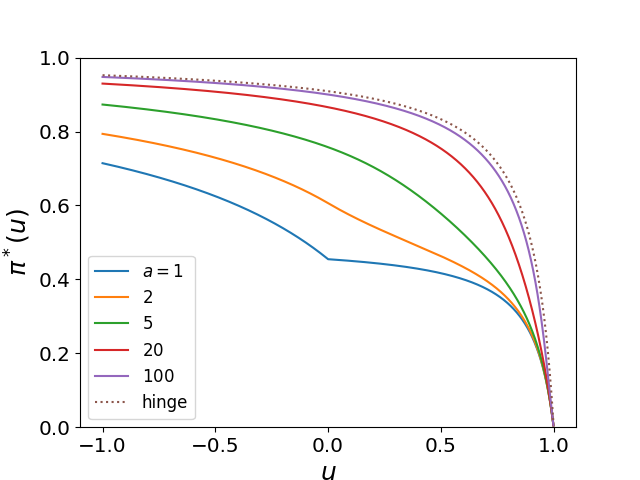
Figure 1: Sampling probability function for generalized smooth hinge loss function.

Theorem 3.7

Assume that $\rho^{*}>1$, loss function is generalized smooth hinge loss function, sampling probability function $\pi^{*}$ is such that assumptions in Theorem 3.6 hold, and $n>((a+1)/a)c_{a,\rho}R^{2}S^{2}/\beta$. Then, the expected number of sampled points is bounded as

$$\mathbb{E}\left[\sum_{t=1}^{n}\pi^{*}(y_{t}x_{t}^{\top}\theta_{t})\right]\leq\kappa\max\left\{\frac{\sqrt{\beta c_{a,\rho}}RS}{(\rho-1)\sqrt{a}}\sqrt{n},\frac{c_{a,\rho}R^{2}S^{2}}{\rho-1}\right\}$$

where $\kappa$ is some positive constant.

Note that for any fixed number of points $n$ satisfying the condition of the theorem, the expected number of sampled points is bounded by a constant for every large enough value of parameter $a$. For obtaining the bound in Theorem 3.7, it is essential how the loss function $\ell(u)$ depends on $u$. It can be shown that when $a$ is large enough, then $\ell(u)$ is approximately $1-u$, and otherwise, it is approximately $\frac{a}{2}(1-u)^{2}$, for $0\leq u\leq 1$.

Multi-class classification

It can be shown that conditions for multi-class classification with the set of classes $\mathcal{Y}$ are the same as for binary classification, with $u(x,y,\theta):=x^{\top}\theta_{y}-\max_{y^{\prime}\in\mathcal{Y}\setminus\{y\}}x^{\top}\theta_{y^{\prime}}$, except for an additional factor of $2$ in the left-hand side of the inequality in the first condition (see Lemma A.3 in Appendix). Hence, all the observations remain to hold for multi-class classification case.

Discussion

Conditions in Assumption 3 allow us to obtain convergence rate bounds for linearly separable data for some predictors and loss functions. Specifically, for linear classifiers, loss functions must satisfy certain properties related to hinge loss functions. We discuss this in more details in Appendix A.7. We next show a framework that allows for deriving convergence rate guarantees for more general cases.

3.2 Bernoulli sampling with constant step size: second set of convergence conditions

We consider algorithm (1) where $z_{t}$ is product of a fixed step size $\gamma$ and a Bernoulli random variable $\zeta_{t}$ with mean $\pi(x,y,\theta)$. Let $g_{t}=\zeta_{t}\nabla_{\theta}\ell(x_{t},y_{t},\theta_{t})$, which is random vector because $\zeta_{t}$ is a random variable and $(x_{t},y_{t})$ is a sampled point. The algorithm (1) is a stochastic gradient descent algorithm with respect to an objective function $\tilde{\ell}$ with gradient

$$\nabla_{\theta}\tilde{\ell}(\theta)=\mathbb{E}[\pi(x,y,\theta)\nabla_{\theta}\ell(x,y,\theta)]$$

where the expectation is with respect to $x$ and $y$. This is a key observation that allows us to derive convergence rate results by deploying convergence rate results for stochastic gradient algorithm that are known to hold under various assumptions on function $\tilde{\ell}$, variance of stochastic gradient vector and step size.

Assume that the sampling probability $\pi$ is an increasing function of the conditional expected loss $\ell(x,\theta)=\mathbb{E}_{y}[\ell(x,y,\theta)\mid x]$. With a slight abuse of notation, we denote this probability as $\pi(\ell(x,\theta))$ where $\pi:\mathbb{R}_{+}\rightarrow[0,1]$ is an increasing and continuous function. Let $\Pi$ be the primitive of $\pi$, i.e. $\Pi^{\prime}=\pi$. We then have

$$\tilde{\ell}(\theta)=\mathbb{E}[\Pi(\ell(x,\theta))].$$ (9)

Note that function $\tilde{\ell}(\theta)$ inherits some properties of functions $\ell(x,y,\theta)$, for $(x,y)\in\mathcal{X}\times\mathcal{Y}$. For example, if $\ell(x,y,\theta)$ is a convex function, for every $(x,y)\in\mathcal{X}\times\mathcal{Y}$, then $\tilde{\ell}$ is a convex function.

The framework for establishing convergence rates allows us to accommodate different sampling strategies and loss functions. For example, it accommodates binary classification for common choice of binary cross-entropy loss function and sampling proportional to absolute error loss, as shown in the following.

Consider binary classification with the prediction probability of positive label $\sigma(x^{\top}\theta)$, where $\sigma:\mathbb{R}_{+}\rightarrow[0,1]$ is an increasing function and $\sigma(-u)+\sigma(u)=1$ for all $u\in\mathbb{R}$. The absolute error loss takes value $1-\sigma(x^{\top}\theta)$ if $y=1$ or value $\sigma(x^{\top}\theta)$ if $y=-1$, which corresponds to $1-\sigma(yx^{\top}\theta)$. The binary cross-entropy loss for a point $(x,y)$ under model parameter $\theta$ can be written as $\ell(x,y,\theta)=-\log(\sigma(yx^{\top}\theta))$. Hence, absolute error loss-based sampling corresponds to the sampling probability function $\pi(x)=1-e^{-x}$.

The following lemma allows to derive convergence rate results for expected loss with respect to loss function $\ell$ by applying known convergence rate results for expected loss with respect to loss function $\tilde{\ell}$ (which is the underlying objective function for stochastic gradient descent algorithm (1) for loss-based sampling).

Lemma 3.8

Assume that for algorithm (1) with loss-based sampling according to $\pi$, for some functions $f_{1},\ldots,f_{m}$, we have

$$\mathbf{E}\left[\frac{1}{n}\sum_{t=1}^{n}\tilde{\ell}(\theta_{t})\right]\leq\inf_{\theta}\tilde{\ell}(\theta)+\sum_{i=1}^{m}f_{i}(n).$$ (10)

Then, it holds

$$\mathbf{E}\left[\frac{1}{n}\sum_{t=1}^{n}\ell(\theta_{t})\right] \leq \inf_{\theta}\Pi^{-1}(\tilde{\ell}(\theta))+\sum_{i=1}^{m}\Pi^{-1}(f_{i}(n)).$$

Table 1: Examples of sampling probability functions.

$\pi(x)$	$\Pi(x)$	$\Pi^{-1}(x)$
$1-e^{-x}$	$x+e^{-x}-1$	$\approx\sqrt{2x}$ for small $x$
$\min\{x,1\}$	$\left\{\begin{array}[]{ll}\frac{1}{2}x^{2}&x\leq 1\\ x-\frac{1}{2}&x\geq 1\end{array}\right.$	$\left\{\begin{array}[]{ll}\sqrt{2x}&x\leq 1/2\\ x+\frac{1}{2}&x\geq 1/2\end{array}\right.$
$\min\{(x/b)^{a},1\}$, $a>0,b>0$	$\left\{\begin{array}[]{ll}\frac{1}{b^{a}(1+a)}x^{1+a}&x\leq a\\ x-\frac{a}{1+a}&x\geq a\end{array}\right.$	$\left\{\begin{array}[]{ll}b^{\frac{a}{1+a}}(1+a)^{\frac{1}{1+a}}x^{\frac{1}{1+a}}&x\leq\frac{b}{1+a}\\ x+\frac{a}{1+a}b&x\geq\frac{b}{1+a}\end{array}\right.$
$1-\frac{1}{1+\mu x}$	$x-\frac{1}{\mu}\log(1+\mu x)$	$\approx\sqrt{(2/\mu)x}$ for small $x$
$1-\frac{1}{1+\mu\sqrt{x}}$	$x-\frac{2}{\mu}\sqrt{x}+\frac{2}{\mu^{2}}\log(1+\mu\sqrt{x})$	$\approx(((3/2)/\mu)x)^{2/3}$ for small $x$

We apply Lemma 3.8 to obtain the following convergence rate guarantee.

Theorem 3.9

Assume that $\ell$ is a convex function, $\tilde{\ell}$ is $L$-smooth, $\Theta_{0}$ is a convex set, $S=\sup_{\theta\in\Theta_{0}\cap\Theta}||\theta-\theta_{1}||$, and $\mathbb{E}[\pi(\ell(x,\theta))||\nabla_{\theta}\ell(x,y,\theta)||^{2}]-||\nabla_{\theta}\tilde{\ell}(\theta)||^{2}\leq\sigma_{\pi}^{2}$. Then, algorithm (1) with $\gamma=1/(L+(\sigma/R)\sqrt{n/2})$,

$$\mathbb{E}[\ell(\bar{\theta}_{n})]\leq\mathbb{E}\left[\frac{1}{n}\sum_{t=1}^{n}\ell(\theta_{t})\right]$$

$$\leq \inf_{\theta}\Pi^{-1}(\tilde{\ell}(\theta))+\Pi^{-1}\left(\frac{\sqrt{2}S\sigma_{\pi}}{\sqrt{n}}\right)+\Pi^{-1}\left(\frac{LS^{2}}{n}\right).$$

Note that the bound on expected loss in Theorem 3.8 depends on $\pi$ through $\Pi^{-1}$ and $\sigma_{\pi}^{2}$. Obviously, we have a bound depending on $\pi$ only through $\Pi^{-1}$ by upper bounding $\sigma_{\pi}^{2}$ with $\sup_{\theta\in\Theta_{0}}\mathbb{E}[||\nabla_{\theta}\ell(x,y,\theta)||^{2}]$.

For convergence rates for large values of number of points $n$, the bound in Theorem 3.8 crucially depends on how $\Pi^{-1}(x)$ behaves for small values of $x$. In Table 1, we show $\Pi$ and $\Pi^{-1}$ for several examples of sampling probability function $\pi$. For all examples in the table, $\Pi^{-1}(x)$ is sub-linear in $x$ for small $x$. For instance, for absolute error loss sampling under binary cross-entropy loss function, $\pi(x)=1-e^{-x}$, $\Pi^{-1}(x)$ is approximately $\sqrt{2x}$ for small $x$. For this case, we have the following corollary.

Corollary 3.10

Under assumptions of Theorem 3.9, sampling probability $\pi(x)=1-e^{-x}$, and $n\geq\max\left\{\left(\frac{16}{9}\right)^{2}2S\sigma_{\pi}^{2},\frac{16}{9}LS^{2}\right\}$ it holds

$$\mathbb{E}[\ell(\bar{\theta}_{n})]\leq\mathbb{E}\left[\frac{1}{n}\sum_{t=1}^{n}\ell(\theta_{t})\right]$$

$$\leq \inf_{\theta}\Pi^{-1}(\tilde{\ell}(\theta))+2^{5/4}\sqrt{S\sigma_{\pi}}\frac{1}{\sqrt[4]{n}}+2\sqrt{L}S\frac{1}{\sqrt{n}}.$$

By using a bound on the expected total loss, we can bound the expected total number of sampled points under certain conditions as follows.

Lemma 3.11

The following bounds hold:

1. Assume that $\pi$ is a concave function, then $\mathbb{E}\left[\sum_{t=1}^{n}\pi(\ell(x_{t},\theta_{t}))\right]\leq\pi\left(\mathbb{E}\left[\frac{1}{n}\sum_{t=1}^{n}\ell(\theta_{t})\right]\right)n.$

2. Assume that $\pi$ is $K$-Lipschitz or that for some $K>0$, $\pi(\ell)\leq\min\{K\ell,1\}$ for all $\ell\geq 0$, then $\mathbb{E}\left[\sum_{t=1}^{n}\pi(\ell(x_{t},\theta_{t}))\right]\leq\min\left\{K\mathbb{E}\left[\sum_{t=1}^{n}\ell(\theta_{t})\right],n\right\}.$

We remark that $\pi$ is a concave function for all examples in Table 1 without any additional conditions, except for $\pi(\ell)=\min\{(\ell/b)^{a},1\}$ which is concave under assumption $0<a\leq 1$. We remark also that for every example in Table 1 except the last one, $\pi(\ell)\leq\min\{K\ell,1\}$ for some $K>0$. Hence, for all examples in Table 1, we have a bound for the expected number of sampled points provided we have a bound for the expected loss.

3.3 Bernoulli sampling with stochastic Polyak’s step size: new algorithm

In this section we propose a new algorithm that combines a Bernoulli sampling and an adaptive stochastic gradient descent update, and provide a convergence rate guarantee. The algorithm is defined as the stochastic gradient descent algorithm (1) with stochastic step size $z_{t}$ being a binary random variable that takes value $\gamma_{t}:=\zeta(x_{t},y_{t},\theta_{t})/\pi(x_{t},y_{t},\theta_{t})$ with probability $\pi(x_{t},y_{t},\theta_{t})$ and takes value $0$ otherwise, where $\pi$ is some function and if $||\nabla_{\theta}\ell(x,y,\theta)||>0$,

$$\zeta(x,y,\theta)=\beta\min\left\{\frac{1}{\psi(x,y,\theta)},\rho\right\}$$

and, $\zeta(x,y,\theta)=0$, otherwise, for some constants $\beta,\rho>0$ and

$$\psi(x,y,\theta):=\frac{||\nabla_{\theta}\ell(x,y,\theta)||^{2}}{\ell(x,y,\theta)-\inf_{\theta^{\prime}}\ell(x,y,\theta^{\prime})}.$$

The expected step size $\zeta(x,y,\theta)$ corresponds to the adaptive step size proposed by (Loizou et al., 2021). When $\pi(x,y,\theta)=1$ for all $x,y,\theta$, then the algorithm boils down to adaptive step size algorithm by Loizou et al. (2021). Our algorithm adds a sampling component and re-weighting of the update such that the step size remains according to stochastic Polyak’s step size in expectation. For many loss functions $\inf_{\theta^{\prime}}\ell(x,y,\theta)=0$, for every $x,y$. In these cases, $\psi(x,y,\theta)=||\nabla_{\theta}\ell(x,y,\theta)||^{2}/\ell(x,y,\theta)$. For instance, for binary cross-entropy loss function, $\inf_{\theta^{\prime}}\ell(x,y,\theta)=\inf_{\theta^{\prime}}(-\log(\sigma(yx^{\top}\theta^{\prime})))=0$, for all $x,y$.

We next show a convergence rate guarantee.

Lemma 3.12

Assume that $\ell$ is a convex, $L$-smooth function, there exists $\Lambda^{*}$ such that $\mathbb{E}[\ell(x,y,\theta^{*})]-\mathbb{E}[\inf_{\theta}\ell(x,y,\theta)]\leq\Lambda^{*}$, and the sampling probability function $\pi$ is such that, for some constant $c\in(0,1)$, for all $x,y,\theta$ such that $||\nabla_{\theta}\ell(x,y,\theta)||>0$,

$$\pi(x,y,\theta)\geq\frac{\beta}{2(1-c)}\min\left\{\rho\psi(x,y,\theta),1\right\}.$$ (11)

Then, we have

$$\mathbb{E}\left[\frac{1}{n}\sum_{t=1}^{n}(\ell(x_{t},y_{t},\theta_{t})-\ell(x_{t},y_{t},\theta^{*}_{t}))\right]$$

$$\leq \frac{\rho\beta}{c\kappa}\Lambda^{*}+\frac{1}{2c\kappa}||\theta_{1}-\theta^{*}||^{2}\frac{1}{n}$$

where $\kappa=\beta\min\{1/(2L),\rho\}$ and $\theta_{t}^{*}$ is a minimizer of $\ell(x_{t},y_{t},\theta^{\prime})$ over $\theta^{\prime}$.

By taking $\rho=1/(2L)$, the bound on the expected average loss boils down to $\Lambda^{*}/c+(L/(c\beta))||\theta_{1}-\theta^{*}||^{2}/n$.

We remark that under condition on the sampling probability in Lemma 3.12, the convergence rate is of the order $O(1/n)$. Similar bound was known to hold for stochastic gradient descent with adaptive stochastic Polyak step size for the finite-sum problem, e.g. see Theorem 3.4 in Loizou et al. (2021). Lemma 3.12 applies to stream-based stochastic gradient descent algorithm, and importantly, allows for Bernoulli sampling with sampling probability function $\pi$.

We next show some instances of $\pi$ that satisfy condition (11) in Lemma 3.12.

Constant sampling probability

Assume that $\kappa\leq 2(1-c)$ and sampling probability function $\pi$ is constant with value at least $\frac{\kappa}{2(1-c)}$. Then, the expected loss bound in Lemma 3.12 holds.

Power function of the expected step size

Consider $\pi$ defined as

$$\pi(x,y,\theta)=\zeta(x,y,\theta)^{\eta}$$ (12)

where $\eta\geq 0$ and $\rho\beta\in(0,1]$. This sampling probability function is an increasing function of $1/\psi(x,y,\theta)$, i.e. $(\ell(x,y,\theta)-\inf_{\theta^{\prime}}\ell(x,y,\theta))/||\nabla_{\theta}\ell(x,y,\theta)||^{2}$. In other words, the sampling probability is an increasing function of the loss normalized by the squared norm of the gradient. Assume that

$$\beta^{1-\eta}\leq 2(1-c)\left(\frac{1}{2L}\right)^{\eta}.$$ (13)

Then, the loss bound in Theorem 3.12 holds.

Linear classifiers: binary classification

For linear classifiers, $||\nabla_{\theta}\ell(x,y,\theta)||^{2}/\ell(x,y,\theta)=h(yx^{\top}\theta)||x||^{2}$ where $h(u)=\ell^{\prime}(u)^{2}/\ell(u)$ which plays a pivotal role in condition (11). For condition (11) to hold, it suffices that

$$\pi(x,y,\theta)\geq\frac{\beta}{2(1-c)}\min\left\{\rho R^{2}h(yx^{\top}\theta),1\right\}.$$

Note that if $\ell(u)$ is an $L^{\prime}$-smooth function in $u$, $\ell(yx^{\top}\theta)$ is an $L^{\prime}||x||^{2}$-smooth function in $\theta$. Taking $\rho=1/(2L)$ with $L=L^{\prime}R^{2}$, we have $\rho R^{2}=1/(2L^{\prime})$.

For logistic regression and binary cross-entropy loss function, we have

$$h(u)=\frac{1}{(1+e^{u})^{2}\log(1+e^{-u})}$$ (14)

which is increasing in $u$ for $u\leq 0$ and is decreasing in $u$ otherwise. Note that $h(u)=(1-e^{-\ell(u)})^{2}/\ell(u)$. By certain properties of function $h$, deferred to Appendix A.13, we have the following two facts: (a) Condition of Lemma 3.12 is satisfied with $\rho=1/(2L)$, by sampling proportional to absolute error loss $\pi^{*}(u)=\omega(1-\sigma(u))$ with $\beta/(4(1-c)L^{\prime})\leq\omega\leq 1$, and (b) Condition of Lemma 3.12 is satisfied by uncertainty sampling according to, for any fixed $a\in(0,1/2]$,

$$\pi^{*}(u)=\frac{\beta}{2(1-c)}\min\left\{\rho R^{2}\frac{1}{H(a)+(1-a)|u|},1\right\}$$

where $H(a)=a\log(1/a)+(1-a)\log(1/(1-a))$.

Linear classifiers: multi-class classification

Condition (11) in Lemma 3.12 can be shown to hold for some loss and uncertainty-based sampling methods. For space reasons, this is deferred to Appendix A.15.

4 Numerical results

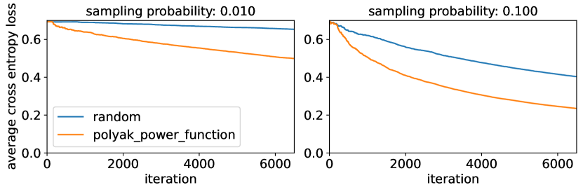
Figure 2: Average cross-entropy progressive loss of Polyak’s step size Loizou et al. (2021) compared to SGD with constant step size. Under scenarios of sampling 1% and 10% sampling from the mushrooms data.

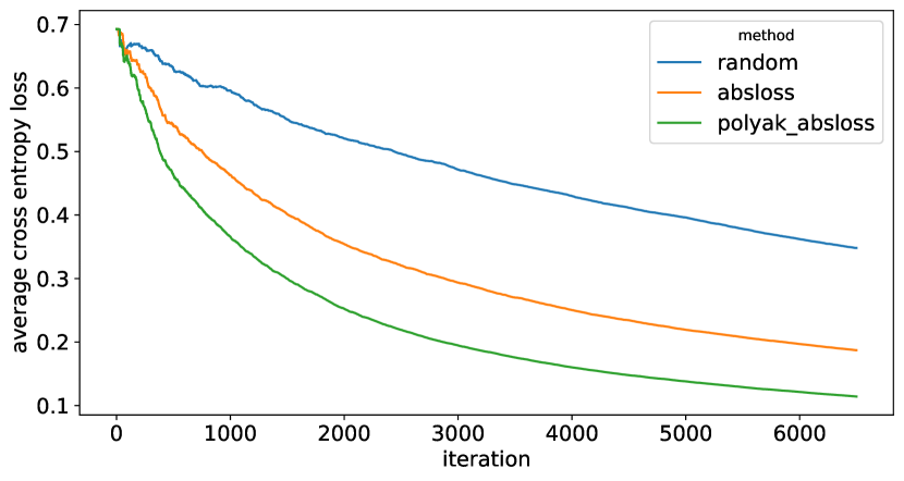
Figure 3: Convergence in terms of average cross-entropy progressive loss of random sampling, loss-based sampling based on the absolute error loss, and our proposed adaptive step size variant of absolute error loss sampling.

We follow Loizou et al. (2021) by using the mushroom classification dataset (Chang and Lin, 2011) and considering binary classification using RBF kernels and logistic regression. This dataset has $n=6499$ instances and $d=6499$ dimensions. In our training procedure, we intentionally limit the training to a single epoch. During this epoch, we process each data instance sequentially, calculating the loss for every individual instance and subsequently updating the model’s weights. This procedure is referred to as progressive validation (Blum et al., 1999) and it allows us to monitor the evolution of the average loss. The restriction to a single epoch ensures that we compute losses only for instances that haven’t influenced model weights. For each of the sampling schemes we run a hyper-parameter sweep aimed at minimising the average progressive loss.

Loizou et al. (2021) showed that stochastic gradient descent with step size corresponding to stochastic Polyak’s step size (SPS) (Loizou et al., 2021) converges faster than gradient descent. Figure 2 shows that these results generalise to settings where we selectively sample from the data set rather than train on the full data set, and step size is according to stochastic Polyak’s step size only in expectation.

Figure 3 shows that our proposed active learning algorithm with adaptive Polyak step size according to SPS and sampling according to $\pi(x)=1-e^{-x}$ leads to faster convergence than the traditional loss based sampling approach. The figure also shows that the traditional loss-based sampling approach converges faster than random sampling.

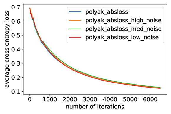
Figure 4: Robustness of the proposed sampling approach with adaptive Polyak’s step size for different variance $\mathrm{var}[\hat{\ell}_{\mathrm{abs}}]=\ell^{2}_{\mathrm{abs}}(1-\ell_{\mathrm{abs}})/(\alpha+\ell_{\mathrm{abs}})$ noise levels of absolute error loss estimator: (low) $\alpha=100$, (medium) $\alpha=2.5$, and (high) $\alpha=1$.

We also simulate a noisy estimator of the absolute error loss for the proposed loss-based sampling with adaptive Polyak’s step size. We model an unbiased noisy estimator $\hat{\ell}_{\mathrm{abs}}$ of the absolute error loss $\ell_{\mathrm{abs}}\in[0,1]$ as a random variable with the beta distribution with parameters $\alpha$ and $\beta$, set such that $\mathbb{E}[\hat{\ell}_{\mathrm{abs}}]=\ell_{\mathrm{abs}}$. The variance of the noise can be controlled by tuning parameter $\alpha$, as we have $\mathrm{var}[\hat{\ell}_{\mathrm{abs}}]=\frac{\ell^{2}_{\mathrm{abs}}(1-\ell_{\mathrm{abs}})}{\alpha+\ell_{\mathrm{abs}}}$. We sweep through a wide range of values $\alpha\geq 1$ and show that the convergence results are robust against the noise in estimating absolute error loss (Figure 4).

5 Conclusion

In this paper, we have shown convergence rate guarantees for loss and uncertainty-based active learning algorithms under various assumptions. We have proposed a new algorithm that combines sampling with stochastic Polyak’s step size and have shown that this algorithm has a convergence rate guarantee under a condition on the sampling probability function. For future research, it may be of interest to apply the approaches in this paper to obtain further convergence rate results and pursue a theoretical study of the effect of noise of the loss estimator, used for evaluating the sampling probability function, on the convergence properties of algorithms.

Appendix A MISSING PROOFS AND ADDITIONAL MATERIAL

A.1 Proof of Lemma 3.2

For any $\theta^{*}\in\Theta$ and $t\geq 1$, we have

$$||\theta_{t+1}-\theta^{*}||^{2}=||\theta_{t}-\theta^{*}||^{2}-2z_{t}\nabla_{\theta}\ell(x_{t},y_{t},\theta_{t})^{\top}(\theta_{t}-\theta^{*})+z_{t}^{2}||\nabla_{\theta}\ell(x_{t},y_{t},\theta_{t})||^{2}.$$

Taking expectation in both sides of the equation, conditional on $x_{t}$, $y_{t}$ and $\theta_{t}$, we have

$$\mathbb{E}[||\theta_{t+1}-\theta^{*}||^{2}\mid x_{t},y_{t},\theta_{t}] = ||\theta_{t}-\theta^{*}||^{2}-2\gamma\pi(x_{t},y_{t},\theta_{t})\nabla_{\theta}\ell(x_{t},y_{t},\theta_{t})^{\top}(\theta_{t}-\theta^{*})$$

$$+\gamma^{2}\pi(x_{t},y_{t},\theta_{t})||\nabla_{\theta}\ell(x_{t},y_{t},\theta_{t})||^{2}.$$

Under Assumption 3, we have

$$\mathbb{E}[||\theta_{t+1}-\theta^{*}||^{2}\mid x_{t},y_{t},\theta_{t}]\leq||\theta_{t}-\theta^{*}||^{2}-2\gamma\beta\tilde{\ell}(x_{t},y_{t},\theta_{t})+\gamma^{2}\alpha\tilde{\ell}(x_{t},y_{t},\theta_{t}).$$

Hence, it holds

$$(2\gamma\beta-\gamma^{2}\alpha)\mathbb{E}[\tilde{\ell}(x_{t},y_{t},\theta_{t})]\leq\mathbb{E}[||\theta_{t}-\theta^{*}||^{2}]-\mathbb{E}[||\theta_{t+1}-\theta^{*}||^{2}].$$

Summing over $t$, we have

$$(2\gamma\beta-\gamma^{2}\alpha)\sum_{t=1}^{n}\mathbb{E}[\tilde{\ell}(x_{t},y_{t},\theta_{t})]\leq||\theta_{1}-\theta^{*}||^{2}.$$

By taking $\gamma=\beta/\alpha$, we have

$$\sum_{t=1}^{n}\mathbb{E}[\tilde{\ell}(x_{t},y_{t},\theta_{t})]\leq||\theta_{1}-\theta^{*}||^{2}\frac{\alpha}{\beta^{2}}.$$

The second statement of the lemma follows from the last above inequality and Jensen’s inequality.

A.2 Proof of Theorem 3.4

We first consider the case when sampling is proportional to zero-one loss. We show that conditions of the theorem imply conditions (4) and (5) to hold, for $\tilde{\ell}=\ell_{01}$ and $\pi=\omega\ell_{01}$, which in turn imply conditions (2) and (3) and hence we can apply the convergence result of Lemma 3.2.

Conditions (4) and (5) are equivalent to:

$$\omega\ell^{\prime}(u)^{2}R^{2}\leq\alpha,\hbox{ for every }u\leq 0$$

and

$$\omega(-\ell^{\prime}(u))(\rho^{*}-u)\geq\beta\hbox{ for every }u\leq 0.$$

Since $\ell$ is a convex function $\ell^{\prime}(u)^{2}$ is decreasing in $u$ and $(-\ell^{\prime}(u))(\rho^{*}-u)$ is decreasing in $u$. Therefore, conditions are equivalent to

$$\omega(\lim_{u\rightarrow-\infty}(-\ell^{\prime}(u)))^{2}R^{2}\leq\alpha$$

and

$$\omega(-\ell^{\prime}(0))\rho^{*}\geq\beta.$$

These conditions hold true by taking $\alpha=\omega c_{2}^{2}R^{2}$ and $\beta=\omega c_{1}\rho^{*}$.

We next consider the case when sampling is proportional to absolute error loss. We show that conditions of the theorem imply conditions (4) and (5) to hold, for $\tilde{\ell}=\ell_{01}$ and $\pi=\omega\ell_{\mathrm{abs}}$, which in turn imply conditions (2) and (3) and hence we can apply the convergence result of Lemma 3.2.

Conditions (4) and (5) correspond to

$$2\omega(-\ell^{\prime}(u))^{2}R^{2}\leq\alpha\hbox{ for every }u<0\hbox{ and }\omega(-\ell^{\prime}(0))^{2}R^{2}\leq\alpha$$

and

$$2\omega(-\ell^{\prime}(u))(\rho^{*}-u)\geq\beta\hbox{ for every }u<0\hbox{ and }\omega(-\ell^{\prime}(0))\rho^{*}\geq\beta.$$

Again, since $(-\ell^{\prime}(u))^{2}$ is decreasing in $u$ and $(-\ell^{\prime}(u))(\rho^{*}-u)$ is decreasing in $u$, it follows that the conditions are equivalent to

$$2\omega(\lim_{u\rightarrow-\infty}(-\ell^{\prime}(u)))^{2}R^{2}\leq\alpha$$

and

$$\omega(-\ell^{\prime}(0))\rho^{*}\geq\beta.$$

Hence, conditions (4) and (5) hold by taking $\alpha=2\omega c_{2}^{2}R^{2}$ and $\beta=\omega c_{1}\rho^{*}$.

A.3 Proof of Theorem 3.5

We show that conditions of the theorem imply conditions (4) and (5) to hold, for $\tilde{\ell}=\ell$, which in turn imply conditions (2) and (3) and hence we can apply the convergence result of Lemma 3.2.

We first consider condition (2). For squared hinge loss function $\ell$ and $\tilde{\ell}=\ell$, clearly condition (2) holds for every $u\geq 1$ as in this case both side of the inequality are equal to zero. For every $u\leq 1$,

$$\frac{\ell(u)}{\ell^{\prime}(u)^{2}}=\frac{1}{2}.$$

Since by assumption $\pi(u)\leq\beta/2$ for all $u$, condition $\alpha/\beta\geq R^{2}$ implies condition (2).

We next consider condition (3). Again, clearly, condition holds for every $u\geq 1$ as in this case both sides of the inequality are equal to zero. For $u\leq 1$, we can write (3) as follows

$$\pi(u)\geq\beta\frac{\ell(u)}{(-\ell^{\prime}(u))(\rho^{*}-u)} = \frac{\beta}{2}\frac{1-u}{\rho^{*}-u}$$

$$= \frac{\beta}{2}\left(1-\frac{1}{1+(1/(\rho^{*}-1))(1-u)}\right)$$

$$= \frac{\beta}{2}\left(1-\frac{1}{1+(\sqrt{2}/(\rho^{*}-1))\sqrt{\ell(u)}}\right).$$

This condition is implied by $\pi(u)\geq\pi^{*}(\ell(u))$ where

$$\pi^{*}(\ell)=\frac{\beta}{2}\left(1-\frac{1}{1+\mu\sqrt{\ell}}\right)$$

with $\mu\geq\sqrt{2}/(\rho^{*}-1)$.

The result of the theorem follows from Lemma 3.2 with $\alpha/\beta=R^{2}$, $0<\beta\leq 2$ and $\pi(u)\geq\pi^{*}(\ell(u))$ for all $u\leq 1$.

For the expected number of samples we proceed as follows. First by concavity and monotonicity of function $\pi^{*}$ and the expected loss bound, we have

$$\mathbb{E}\left[\sum_{t=1}^{n}\pi^{*}(\ell(x_{t},y_{t},\theta_{t}))\right]\leq\pi^{*}\left(\mathbb{E}\left[\frac{1}{n}\sum_{t=1}^{n}\ell(x_{t},y_{t},\theta_{t})\right]\right)n\leq\pi^{*}\left(\frac{||\theta_{1}-\theta^{*}||^{2}R^{2}}{\beta n}\right)n.$$

Then, combined with the fact $\pi^{*}(v)\leq\frac{\beta\mu}{2}\sqrt{v}$ for all $v\geq 0$, it follows

$$\mathbb{E}\left[\sum_{t=1}^{n}\pi^{*}(\ell(x_{t},y_{t},\theta_{t}))\right]\leq||\theta_{1}-\theta^{*}||\frac{\mu\sqrt{\beta}}{2}\sqrt{n}.$$

Since $\pi^{*}(v)\leq\beta/2$ for all $v$, it obviously holds $\mathbb{E}\left[\sum_{t=1}^{n}\pi^{*}(\ell(x_{t},y_{t},\theta_{t}))\right]\leq(\beta/2)n$, which completes the proof of the theorem.

A.4 Proof of Theorem 3.6

Assume that $\pi^{*}$ is such that for given $\rho\in(1,\rho^{*}]$, $\pi^{*}(u)(-\ell^{\prime}(u))(\rho-u)=\beta\ell(u)$ for all $u\in\mathbb{R}$. Then, $\pi^{*}$ satisfies equation (5) for all $u\in\mathbb{R}$. Note that

$$\pi^{*}(u)=\beta\frac{\ell(u)}{(-\ell^{\prime}(u))(\rho-u)}=\left\{\begin{array}[]{ll}\beta\frac{\frac{a}{a+1}-u}{\rho-u}&\hbox{ if }u\leq 0\\ \beta\left(\frac{a}{a+1}\frac{1}{1-u^{a}}(1-u)-\frac{1}{a+1}u\right)\frac{1}{\rho-u}&\hbox{ if }0\leq u\leq 1\\ 0&\hbox{ if }u\geq 1.\end{array}\right.$$

By condition (4), we must have

$$\frac{-\ell^{\prime}(u)}{\rho-u}\leq\frac{\alpha}{\beta R^{2}}.$$

Note that

$$\ell^{\prime}(u)=\left\{\begin{array}[]{ll}-1&\hbox{ if }u\leq 0\\ -(1-u^{a})&\hbox{ if }0\leq u\leq 1\\ 0&\hbox{ otherwise}.\end{array}\right.$$

Hence, for every $u\leq 0$, it must hold

$$\frac{1}{\rho-u}\leq\frac{\alpha}{\beta R^{2}}$$

which is equivalent to $\alpha/\beta\leq R^{2}/\rho$. For every $0\leq u\leq 1$, it must hold

$$f_{a}(u):=\frac{1-u^{a}}{\rho-u}\leq\frac{\alpha}{\beta R^{2}}.$$

Thus, it must hold $\alpha/\beta\geq c_{a,\rho}R^{2}$ where $c_{a,\rho}=\sup_{u\in[0,1]}f_{a}(u)$.

Function $f_{a}$ has boundary values $f_{a}(0)=1/\rho$ and $f_{a}(1)=0$. Furthermore, note

$$f_{a}^{\prime}(u)=\frac{1+(a-1)u^{a}-\rho au^{a-1}}{(\rho-u)^{2}}.$$

Note $f_{a}(0)=1/{\rho}^{2}>0$ and $f_{a}^{\prime}(1)=-(\rho-1)a<0$. Let $u_{*}$ be such that $f_{a}^{\prime}(u_{*})=0$, which holds if, and only if, $g_{a}(u_{*}):=(a-1){u_{*}}^{a}-\rho a{u_{*}}^{a-1}+1=0$.

Note that

$$c_{a,\rho}=\sup_{u\in[0,1]}f_{a}(u)=f_{a}(u_{*})=au_{*}^{a-1}.$$

For $a=1$, $f_{1}$ is decreasing on $[0,1]$ hence $c_{1,\rho}=f_{1}(0)=1/\rho$. For $a=2$, $u_{*}$ is a solution of a quadratic equation, and it can be readily shown that $c_{2,\rho}=2\rho(1-\sqrt{{\rho}^{2}-1})$. For every $a\geq 1$, we have $c_{a,\rho}\leq a/(1+a(\rho-1))$. This obviously holds with equality for $a=1$, hence it suffices to show that the inequality holds for $a>1$.

Consider the case $a>1$. Note that $g_{a}(u_{*})=0$ is equivalent to

$$au_{*}^{a-1}=\frac{1}{\rho-\frac{a-1}{a}u_{*}}.$$ (15)

Combined with the fact $u_{*}\in[0,1]$, it immediately follows

$$au_{*}^{a-1}\leq\frac{a}{a(\rho-1)+1}.$$

Furthermore, note that $\lim_{a\rightarrow\infty}c_{a,\rho}=1/(\rho-1)$. To see this, consider (15). Note that $u_{*}$ goes to $1$ as $a$ goes to infinity. This can be shown by contradiction as follows. Assume that there exists a constant $c\in[0,1)$ and $a_{0}$ such that $u_{*}\leq c$ for all $a\geq a_{0}$. Then, from (15), $ac^{a-1}\geq 1/\rho^{*}$. The left-hand side in the last inequality goes to $0$ as $a$ goes to infinity while the right-hand side is a constant greater than zero, which yields a contradiction. From (15), it follows that $au_{*}^{a-1}$ goes to $1/(\rho-1)$ as $a$ goes to infinity.

We prove the second statement of the theorem as follows. It suffices to show that condition (4) holds true as condition (5) clearly holds for every $\pi$ such that $\pi(u)\geq\pi^{*}(u)$ for every $u\in\mathbb{R}$. For condition (4) to hold, it is sufficient that

$$f(u):=\frac{\ell(u)}{\ell^{\prime}(u)^{2}}\geq\frac{\beta R^{2}}{\alpha},\hbox{ for all }u\leq 1.$$

Note that

$$f(u)=\left\{\begin{array}[]{ll}\frac{a}{a+1}-u&\hbox{ if }u\leq 0\\ \frac{1}{a+1}\frac{u^{a+1}-(a+1)u+a}{(1-u^{a})^{2}}&\hbox{ if }0\leq u\leq 1.\end{array}\right.$$

Function $f$ is a decreasing function. This is obviously true for $u\leq 0$. For $0\leq u\leq 1$, we show this as follows. Note that

$$f^{\prime}(u)=\frac{2au^{2a}-(2a-1)(a+1)u^{a}+2a^{2}u^{a-1}-(a+1)}{(a+1)(1-u^{a})^{3}}.$$

Hence, $f^{\prime}(u)\leq 0$ is equivalent to

$$2au^{a-1}(u^{a+1}+a)\leq(a+1)(1-(2a-1)u^{a}).$$

In the last inequality, the left-hand side is increasing in $u$ and the right-hand side is decreasing in $u$. Hence the inequality holds for every $u\in[0,1]$ is equivalent to the inequality holding for $u=1$. For $u=1$, the inequality holds with equality.

Note that

$$f(1) = \frac{0}{0}$$

$$= \frac{1}{a+1}\frac{(a+1)u^{a}-(a+1)}{-2(1-u^{a})au^{a-1}}|_{u=1}=\frac{0}{0}$$

$$= \frac{1}{a+1}\frac{(a+1)au^{a-1}}{2a^{2}u^{2(a-1)}-2(1-u^{a})a(a-1)u^{a-2}}|_{u=1}=\frac{1}{a+1}\frac{(a+1)a}{2a^{2}}$$

$$= \frac{1}{2a}.$$

It follows that $\inf_{u\leq 1}f(u)=f(1)=\frac{1}{2a}\leq\alpha/(\beta R^{2})$, hence it is suffices that $\alpha/\beta\geq R^{2}/(2a)$.

A.5 Proof of Theorem 3.7

Lemma A.1

For every $a\geq 1$,

$$\pi^{*}(u)\leq\pi^{**}(u)=\beta\frac{1-u}{\rho-1}\hbox{ for every }u\leq 1.$$

Proof

For $u\leq 1$, $\pi^{*}(u)=\beta(a/(a+1)-u)/(\rho-u)$, so obviously, $\pi^{*}(u)\leq\beta(1-u)/(\rho-u)$. For $0\leq u\leq 1$, we show that next that $a(1-u)/(1-u^{a})-u\leq a(1-u)$, which implies that $\pi^{*}(u)\leq(a/(a+1))\beta(1-u)/(\rho-u)$. To show the asserted inequality, by straightforward calculus it can be shown that the inequality is equivalent to $(1-(1-u))^{1-a}\geq 1-(1-a)(1-u)$ which clearly holds true.

$\hfill\blacksquare$

Lemma A.2

For every $c\in(1,6/5)$, for every $0\leq u\leq 1$, if $(a+1)(1-u)\geq c$, then

$$\ell(u)\geq\left(1-\frac{1}{c}\right)(1-u)$$

and, otherwise,

$$\ell(u)\geq\left(1-\frac{1}{3}\frac{c}{1-c/2}\right)\frac{a}{2}(1-u)^{2}.$$

Proof

We first show the first inequality. For $u\leq 1$, it clearly holds $\ell(u)\leq 1-u$, and

$$\frac{\frac{a}{a+1}-u}{1-u}=\frac{1-u-\frac{1}{a+1}}{1-u}=1-\frac{1}{(a+1)(1-u)}$$

thus, for every $c>1$, $\ell(u)\geq(1-1/c)(1-u)$ whenever $(a+1)(1-u)\geq c$.

For $0\leq u<1$, it holds $\ell(u)=1-u-(1/(a+1))(1-u^{a+1})$, hence it clearly holds $\ell(u)\leq 1-u$. Next, note

$$\frac{\ell(u)}{1-u}=1\frac{1-u^{a+1}}{(a+1)(1-u)}\geq 1-\frac{1}{(a+1)(1-u)}.$$

Hence, again, for every $c>1$, $\ell(u)\geq(1-1/c)(1-u)$ whenever $(a+1)(1-u)\geq c$.

We next show the second inequality. For $0<u\leq 1$, note that $\ell^{\prime}(u)=-(1-u^{a})$, $\ell^{\prime\prime}(u)=au^{a-1}$ and $\ell^{\prime\prime\prime}(u)=a(a-1)u^{a-2}$. In particular, $\ell^{\prime}(1)=0$, $\ell^{\prime\prime}(1)=a$ and $\ell^{\prime\prime\prime}(1)=a(a-1)$. By limited Taylor development, for some $u_{0}\in[u,1]$,

$$\ell(u)=\frac{a}{2}(1-u)^{2}-\frac{a(a-1)}{6}u_{0}^{a-2}(1-u)^{3}.$$

From this, it immediately follows that $\ell(u)\leq\frac{a}{2}(1-u)^{2}$ for every $u\leq 1$. For the case $a\geq 2$, we have

$$\ell(u)\geq\frac{a}{2}(1-u)^{2}\left(1-\frac{1}{3}(a-1)(1-u)\right).$$

Hence, for every $c\geq 0$, $\ell(u)\geq\frac{a}{2}(1-u)^{2}(1-c/3)$ whenever $(a+1)(1-u)\leq c$. For $1\leq a\leq 2$, we have

$$\ell(u)\geq\frac{a}{2}(1-u)^{2}\left(1-\frac{1}{3}\frac{(a-1)(1-u)}{u^{2-a}}\right)\geq\frac{a}{2}(1-u)^{2}\left(1-\frac{1}{3}\frac{(a-1)(1-u)}{u}\right).$$

Under $(a+1)(1-u)\leq c$, with $0\leq c<2$, we have

$$\frac{(a-1)(1-u)}{u}\leq\frac{c}{1-\frac{c}{a+1}}\leq\frac{c}{1-\frac{c}{2}}.$$

Hence, it follows

$$\ell(u)\geq\frac{a}{2}(1-u)^{2}\left(1-\frac{1}{3}\frac{c}{1-\frac{c}{2}}\right).$$

$\hfill\blacksquare$

Next, note that for every $x,y,\theta$,

$$\pi^{*}(yx^{\top}\theta)\leq\pi^{**}(yx^{\top}\theta)\leq\frac{\beta}{\rho^{*}-1}(1-yx^{\top}\theta)=\frac{\beta}{\rho^{*}-1}(1-\ell^{-1}(\ell(x,y,\theta)))$$

where $\ell^{-1}$ is the inverse function of $\ell(u)$ for $u<1$ and $\ell^{-1}(0)=0$.

Hence, we have

$$\mathbb{E}\left[\sum_{t=1}^{n}\pi^{*}(y_{t}x_{t}^{\top}\theta_{t})\right] \leq \frac{\beta}{\rho-1}\left(1-\ell^{-1}\left(\mathbb{E}\left[\frac{1}{n}\sum_{t=1}^{n}\ell(x_{t},y_{t},\theta_{t})\right]\right)\right)n$$

$$\leq \frac{\beta}{\rho-1}\left(1-\ell^{-1}\left(c_{a,\rho}\frac{||\theta_{1}-\theta^{*}||^{2}R^{2}}{\beta}\frac{1}{n}\right)\right)n$$

where the first inequality is by concavity of the function $1-\ell^{-1}(\ell)$ and the second inequality is by Theorem 3.6.

To apply Lemma A.2, we need that

$$\ell^{-1}\left(c_{a,\rho}\frac{||\theta_{1}-\theta^{*}||^{2}R^{2}}{\beta}\frac{1}{n}\right)>0$$

which is equivalent to

$$c_{a,\rho}\frac{||\theta_{1}-\theta^{*}||^{2}R^{2}}{\beta}\frac{1}{n}<\ell(0)=\frac{a}{a+1}$$

i.e.

$$n>\frac{a+1}{a}c_{a,\rho}\frac{||\theta_{1}-\theta^{*}||^{2}R^{2}}{\beta}.$$

By Lemma A.2, we can distinguish two cases when

$$1-\ell^{-1}\left(c_{a,\rho}\frac{||\theta_{1}-\theta^{*}||^{2}R^{2}}{\beta}\frac{1}{n}\right)\geq\frac{c}{a+1}$$

or, otherwise, where $c$ is an arbitrary constant in $(1,6/5)$.

In the first case,

$$1-\ell^{-1}\left(c_{a,\rho}\frac{||\theta_{1}-\theta^{*}||^{2}R^{2}}{\beta}\frac{1}{n}\right)\leq c_{1}c_{a,\rho}\frac{||\theta_{1}-\theta^{*}||^{2}R^{2}}{\beta}\frac{1}{n}$$

where $c_{1}=1/(1-1/c)$ while in the second case

$$1-\ell^{-1}\left(c_{a,\rho}\frac{||\theta_{1}-\theta^{*}||^{2}R^{2}}{\beta}\frac{1}{n}\right)\leq c_{2}\sqrt{\frac{2}{a}}\sqrt{c_{a,\rho}\frac{||\theta_{1}-\theta^{*}||^{2}R^{2}}{\beta}\frac{1}{n}}$$

where $c_{2}=1/(1-(1/3)c/(1-c/2)$.

It follows that for some constant $\kappa>0$,

$$\mathbb{E}\left[\sum_{t=1}^{n}\pi^{*}(y_{t}x_{t}^{\top}\theta_{t})\right]\leq\kappa\max\left\{\frac{\sqrt{\beta c_{a,\rho}}}{(\rho-1)\sqrt{a}}||\theta_{1}-\theta^{*}||R\sqrt{n},\frac{c_{a,\rho}}{\rho-1}||\theta_{1}-\theta^{*}||^{2}R^{2}\right\}.$$

A.6 Multi-class classification for linearly separable data

We consider multi-class classification with $k\geq 2$ classes. Let $\mathcal{Y}=\{1,\ldots,k\}$ denote the set of classes. For every $y\in\mathcal{Y}$, let $\theta_{y}\in\mathbb{R}^{d}$ and let $\theta=(\theta_{1}^{\top},\ldots,\theta_{k}^{\top})^{\top}\in\mathbb{R}^{kd}$ be the parameter. For given $x$ and $\theta$, predicted class is an element of $\arg\max_{y\in\mathcal{Y}}x^{\top}\theta_{y}$.

The linear separability condition is defined as follows: there exists $\theta^{*}\in\mathbb{R}^{kd}$ such that for some $\rho^{*}>1$, for every $x\in\mathcal{X}$ and $y\in\mathcal{Y}$,

$$x^{\top}\theta^{*}_{y}-\max_{y^{\prime}\in\mathcal{Y}\setminus\{y\}}x^{\top}{\theta^{*}_{y^{\prime}}}\geq\rho^{*}.$$

Let

$$u(x,y,\theta)=x^{\top}\theta_{y}-\max_{y^{\prime}\in\mathcal{Y}\setminus\{y\}}x^{\top}\theta_{y^{\prime}}.$$

We consider margin loss functions which are according to a decreasing function of $u(x,y,\theta)$, i.e. $\ell(x,y,\theta)\equiv\ell(u(x,y,\theta))$ and $\tilde{\ell}(x,y,\theta)\equiv\tilde{\ell}(u(x,y,\theta))$. For example, this accomodates hinge loss function for multi-class classification Crammer and Singer (2002).

Lemma A.3

Conditions in Assumption 3 hold provided that for every $x$, $y$ and $\theta$,

$$\pi(x,y,\theta)(-\ell^{\prime}(u(x,y,\theta))^{2}2R^{2}\leq\alpha\tilde{\ell}(u(x,y,\theta))$$

and

$$\pi(x,y,\theta)(-\ell^{\prime}(u(x,y,\theta)))(\rho^{*}-u(x,y,\theta))\geq\beta\tilde{\ell}(u(x,y,\theta)).$$

Proof of the lemma

For $x\in\mathcal{X}$ and $y\in\mathcal{Y}$, let $\phi(x,y)=(\phi_{1}(x,y)^{\top},\ldots,\phi_{k}(x,y)^{\top})^{\top}$ where $\phi_{i}(x,y)=x$ if $i=y$ and $\phi_{i}(x,y)$ is the $d$-dimensional null-vector, otherwise. Note that

$$u(x,y,\theta)=\theta^{\top}\phi(x,y)-\frac{1}{|\mathcal{Y}^{*}(x,y,\theta)|}\sum_{y^{\prime}\in\mathcal{Y}^{*}(x,y,\theta)}\theta^{\top}\phi(x,y^{\prime})$$ (16)

where

$$\mathcal{Y}^{*}(x,y,\theta)=\arg\max_{y^{\prime}\in\mathcal{Y}^{*}(x,y,\theta)}\theta_{y^{\prime}}^{\top}x.$$

Note that

$$||\nabla_{\theta}\ell(x,y,\theta)||^{2}=\ell^{\prime}(u(x,y,\theta))^{2}||\nabla_{\theta}u(x,y,\theta)||^{2}.$$

From (16),

$$\nabla_{\theta}u(x,y,\theta)=\phi(x,y)-\frac{1}{|\mathcal{Y}^{*}(x,y,\theta)|}\sum_{y^{\prime}\in\mathcal{Y}^{*}(x,y,\theta)}\phi(x,y^{\prime}).$$

It can be readily shown that

$$||\nabla_{\theta}u(x,y,\theta)||^{2}=\left(1+\frac{1}{|\mathcal{Y}^{*}(x,y,\theta)|}\right)||x||^{2}\leq 2||x||^{2}.$$

Hence, we have

$$||\nabla_{\theta}\ell(x,y,\theta)||^{2}\leq 2(-\ell^{\prime}(u(x,y,\theta))^{2}||x||^{2}.$$ (17)

Next, note that $\nabla_{\theta}\ell(x,y,\theta)=\ell^{\prime}(u(x,y,\theta))\nabla_{\theta}u(x,y,\theta)$,

$$\nabla_{\theta}\ell(x,y,\theta)^{\top}(\theta-\theta^{*})=(-\ell^{\prime}(u(x,y,\theta)))\nabla_{\theta}u(x,y,\theta)^{\top}(\theta^{*}-\theta).$$

and

$$\nabla_{\theta}u(x,y,\theta)^{\top}\theta^{*}=x^{\top}\theta^{*}_{y}-\max_{y^{\prime}\in\mathcal{Y}\setminus\{y\}}x^{\top}{\theta^{*}_{y^{\prime}}}\geq\rho^{*}.$$

It follows

$$\nabla_{\theta}\ell(x,y,\theta)^{\top}(\theta-\theta^{*})\geq(-\ell^{\prime}(u(x,y,\theta))(\rho^{*}-u(x,y,\theta)).$$ (18)

Using (17) and (18), for conditions (2) and (3) to hold, it suffices that

$$\pi(x,y,\theta)(-\ell^{\prime}(u(x,y,\theta)))^{2}2R^{2}\leq\alpha\tilde{\ell}(u(x,y,\theta))$$

and

$$\pi(x,y,\theta)(-\ell^{\prime}(u(x,y,\theta))(\rho^{*}-u(x,y,\theta))\geq\beta\tilde{\ell}(u(x,y,\theta)).$$

Note that these conditions are equivalent to those for the binary case in (4) and (5) except for an additional factor $2$ in the first of the last above inequalities.

$\hfill\blacksquare$

A.7 Implications of conditions (4) and (5)

We discuss some implications of conditions (4) and (5). Some of this discussion will tell us about loss functions for which conditions cannot be applied.

First, we note that $\tilde{\ell}(u)>0$ implies $\pi(u)>0$. Hence, equivalently, $\pi(u)=0$ implies $\tilde{\ell}(u)=0$.

Second, we note that under conditions (4) and (5) it is necessary that for all $u\in\mathbb{R}$, either

$$-\ell^{\prime}(u)\leq\frac{\alpha}{\beta R^{2}}\max\{\rho^{*}-u,0\}\hbox{ or }\pi(u)=0.$$

Hence, whenever $\tilde{\ell}(u)>0$ (and thus $\pi(u)>0$), then $-\ell^{\prime}(u)\leq\frac{\alpha}{\beta R^{2}}\max\{\rho^{*}-u,0\}$. The latter condition means that $\ell^{\prime}(u)=0$ whenever $u\geq\rho^{*}$ and otherwise the derivative of $\ell$ at $u$ is bounded such that $\ell^{\prime}(u)\geq-(\alpha/(\beta R^{2}))(\rho^{*}-u)$. In other words, function $\ell$ must not decrease too fast on $(-\infty,\rho^{*}]$.

Third, assume $\ell$ and $\tilde{\ell}$ are such that $\ell(u)=0$ and $\tilde{\ell}(u)=0$ for all $u\geq 1$ and $\tilde{\ell}(u)>0$ for all $u<1$. Then, for every $u\leq 1$

$$\int_{u}^{1}(-\ell(v))dv\leq\frac{\alpha}{\beta R^{2}}\int_{u}^{1}(\rho^{*}-v)dv$$

which by integrating is equivalent to

$$\ell(u)\leq\frac{\alpha}{\beta R^{2}}\left((\rho^{*}-1)(1-u)+\frac{1}{2}(1-u)^{2}\right).$$

This shows that $\ell$ must be upper bounded by a linear combination of hinge and squared hinge loss function.

Forth, assume that $\pi$ is decreasing in $u$, then for every fixed $u_{0}\in\mathbb{R}$,

$$\tilde{\ell}(u)\geq\frac{\pi(u_{0})R^{2}}{\alpha}(-\ell^{\prime}(u))^{2}\hbox{ for every }u\leq u_{0}.$$

If $\tilde{\ell}=\ell$, then

$$\ell(u)\leq\left(\sqrt{\ell(u_{0})}+\frac{1}{2R}\sqrt{\frac{\alpha}{\pi(u_{0})}}(u_{0}-u)\right)^{2}\hbox{ for all }u\leq u_{0}.$$

Fifth, and last, assume that $\pi$ is an even function and that there exists $c>0$ and $u_{0}\leq\rho^{*}$ such that $\tilde{\ell}(u)\geq c$ for every $u\leq u_{0}$. Then,

$$\pi(u)=\Omega\left(\frac{1}{|u|^{2}}\right)$$

which limits the rate at which $\pi(u)$ is allowed to decrease with $|u|$. To see, this, from conditions (4) and (5), for every $u\leq\rho^{*}$,

$$\tilde{\ell}(u)\leq\frac{\alpha}{\beta^{2}R^{2}}\pi(u)(\rho^{*}-u)^{2}.$$

Hence, $\pi(u)\geq(c\beta^{2}R^{2}/\alpha)/(\rho^{*}-u))$ for every $u\leq u_{0}$. The lower bound is tight in case when $\ell$ is squared hinge loss function and $\tilde{\ell}(u)=c$ for every $u\leq u_{0}<1$. In this case, from conditions (4) and (5), for every $u\leq u_{0}$,

$$c\beta\frac{1}{(1-u)(\rho^{*}-u)}\leq\pi(u)\leq\frac{c\alpha}{R^{2}}\frac{1}{(1-u)^{2}}$$

which implies $\pi(u)=\Theta(1/|u|^{2})$.

A.8 Proof of Lemma 3.8

Function $\Pi$ is a convex function because, by assumption, $\pi$ is an increasing function. By (9 and Jensen’s inequality, we have

$$\mathbb{E}\left[\frac{1}{n}\sum_{t=1}^{n}\tilde{\ell}(\theta_{t})\right] = \mathbb{E}\left[\frac{1}{n}\sum_{t=1}^{n}\Pi(\ell(x_{t},\theta_{t}))\right]$$

$$\geq \Pi\left(\mathbb{E}\left[\frac{1}{n}\sum_{t=1}^{n}\ell(x_{t},\theta_{t})\right]\right)$$

$$= \Pi\left(\mathbb{E}\left[\frac{1}{n}\sum_{t=1}^{n}\ell(x_{t},y_{t},\theta_{t})\right]\right)$$

$$= \Pi\left(\mathbb{E}\left[\frac{1}{n}\sum_{t=1}^{n}\ell(\theta_{t})\right]\right).$$

Therefore, we have

$$\mathbb{E}\left[\frac{1}{n}\sum_{t=1}^{n}\ell(\theta_{t})\right]\leq\Pi^{-1}\left(\mathbb{E}\left[\frac{1}{n}\sum_{t=1}^{n}\tilde{\ell}(\theta_{t})\right]\right).$$

Combined with condition (10), we have

$$\mathbf{E}\left[\frac{1}{n}\sum_{t=1}^{n}\ell(\theta_{t})\right] \leq \Pi^{-1}\left(\inf_{\theta}\tilde{\ell}(\theta)+\sum_{i=1}^{m}f_{i}(n)\right)$$

$$\leq \inf_{\theta}\Pi^{-1}(\tilde{\ell}(\theta))+\sum_{i=1}^{m}\Pi^{-1}(f_{i}(n))$$

where the last inequality holds because $\Pi^{-1}$ is a concave function, and hence, it is a subadditive function.

A.9 Proof of Theorem 3.9

Under assumptions of the theorem, by Theorem 6.3 Bubeck (2015),

$$\mathbb{E}\left[\tilde{\ell}(\bar{\theta}_{n})\right]\leq\mathbb{E}\left[\frac{1}{n}\sum_{t=1}^{n}\tilde{\ell}(\theta_{t})\right]\leq\inf_{\theta}\tilde{\ell}(\theta)+\sqrt{2}S\sigma_{\pi}\frac{1}{\sqrt{n}}+LS^{2}\frac{1}{n}.$$

Combining with Lemma 3.8, we obtain the assertion of the theorem.

A.10 Proof of Corollary 3.10

Lemma A.4

For $\Pi(x)=x-1+e^{-x}$,

$$\Pi^{-1}(y)\leq 2\sqrt{y}\hbox{ for }y\in[0,(3/4)^{2}].$$

Proof

We consider

$$\Pi(x)=x-(1-e^{-x}).$$

By limited Taylor development,

$$1-e^{-x}\leq x=\frac{1}{2}x^{2}+\frac{1}{6}x^{3}.$$

Hence,

$$\Pi(x)\geq\frac{1}{2}x^{2}\left(1-\frac{1}{3}x\right).$$

Note that $\Pi(x)\geq cx^{2}$ for some constant $c>0$ provided that

$$\frac{1}{2}x^{2}\left(1-\frac{1}{3}x\right)\geq cx^{2}$$

which is equivalent to $x\leq 3(1-2c)$. Hence, for any fixed $c\in[0,1/2)$, we have

$$\Pi(x)\geq cx^{2},\hbox{ for every }x\in[0,3(1-2c)].$$

Now, condition $x\leq 3(1-2c)$ is implied by $\sqrt{\Pi(x)/c}\leq 3(1-2c)$, i.e. $\Pi(x)\leq 9c(1-2c)^{2}$. Hence,

$$\Pi^{-1}(y)\leq\sqrt{\frac{1}{c}y}\hbox{ for }y\in[0,9c(1-2c)^{2}].$$

In particular, by taking $c=1/4$, we have

$$\Pi^{-1}(y)\leq 2\sqrt{y}\hbox{ for }y\in[0,(3/4)^{2}].$$

$\hfill\blacksquare$

We have the bound in Theorem 3.9. Under $\sqrt{2}S\sigma_{\pi}/\sqrt{n}\leq(3/4)^{2}$, we have

$$\Pi^{-1}\left(\sqrt{2}S\sigma_{\pi}\frac{1}{\sqrt{n}}\right)\leq 2^{5/4}\sqrt{S\sigma_{\pi}}\frac{1}{\sqrt[4]{n}}.$$

Under $LS^{2}/n\leq(3/4)^{2}$, we have

$$\Pi^{-1}\left(LS^{2}\frac{1}{n}\right)\leq 2\sqrt{L}S\frac{1}{\sqrt{n}}.$$

This completes the proof of the corollary.

A.11 Proof of Lemma 3.12

To simplify notation, we write $\ell_{t}(\theta)\equiv\ell(x_{t},y_{t},\theta)$, $\gamma_{t}=\gamma(x_{t},y_{t},\theta_{t})$ and $\pi_{t}=\pi(x_{t},y_{t},\theta_{t})$.

Since $\ell$ is an $L$-smooth function, we have $\ell(x,y,\theta)-\inf_{\theta^{\prime}}\ell(x,y,\theta^{\prime})\geq 1/(2L^{2})||\nabla_{\theta}\ell(x,y,\theta)||^{2}$. Hence, for any $x,y,\theta$ such that $||\nabla_{\theta}\ell(x,y,\theta)||>0$, we have

$$\frac{\ell(x,y,\theta)-\min_{\theta^{\prime}}\ell(x,y,\theta^{\prime})}{||\nabla_{\theta}\ell(x,y,\theta)||^{2}}\geq\frac{1}{2L}.$$ (19)

Combined with the definition of $\zeta$ and the fact $\zeta(x_{t},y_{t},\theta_{t})=\gamma_{t}\pi_{t}$, we have

$$\kappa:=\beta\min\left\{\frac{1}{2L},\rho\right\}\leq\gamma_{t}\pi_{t}\hbox{ whenever }||\nabla_{\theta}\ell(x,y,\theta)||>0.$$ (20)

From the definition of $\zeta$ and the fact $\zeta(x_{t},y_{t},\theta_{t})=\gamma_{t}\pi_{t}$, we have

$$\gamma_{t}\pi_{t}\leq\rho\beta.$$ (21)

Next, note

$$\mathbb{E}[||\theta_{t+1}-\theta^{*}||^{2}\mid x_{t},y_{t},\theta_{t}] = ||\theta_{t}-\theta^{*}||^{2}-2\mathbb{E}[z_{t}\mid x_{t},y_{t},\theta_{t}]\nabla_{\theta}\ell_{t}(\theta_{t})^{\top}(\theta_{t}-\theta^{*})+\mathbb{E}[z_{t}^{2}\mid x_{t},y_{t},\theta_{t}]||\nabla_{\theta}\ell_{t}(\theta_{t})||^{2}$$

$$= ||\theta_{t}-\theta^{*}||^{2}-2\gamma_{t}\pi_{t}\nabla_{\theta}\ell_{t}(\theta_{t})^{\top}(\theta_{t}-\theta^{*})+\gamma_{t}^{2}\pi_{t}||\nabla_{\theta}\ell_{t}(\theta_{t})||^{2}$$

$$\leq ||\theta_{t}-\theta^{*}||^{2}-2\gamma_{t}\pi_{t}(\ell_{t}(\theta_{t})-\ell_{t}(\theta^{*}))+\gamma_{t}^{2}\pi_{t}\frac{||\nabla_{\theta}\ell_{t}(\theta_{t})||^{2}}{\ell_{t}(\theta_{t})-\ell_{t}(\theta_{t}^{*})}(\ell_{t}(\theta_{t})-\ell_{t}(\theta^{*}_{t}))$$

$$= ||\theta_{t}-\theta^{*}||^{2}-\gamma_{t}\pi_{t}\left(2-\gamma_{t}\frac{||\nabla_{\theta}\ell_{t}(\theta_{t})||^{2}}{\ell_{t}(\theta_{t})-\ell_{t}(\theta_{t}^{*})}\right)(\ell_{t}(\theta_{t})-\ell_{t}(\theta^{*}_{t}))+2\gamma_{t}\pi_{t}(\ell_{t}(\theta^{*})-\ell_{t}(\theta^{*}_{t}))$$

$$\leq ||\theta_{t}-\theta^{*}||^{2}-2c\kappa(\ell_{t}(\theta_{t})-\ell_{t}(\theta^{*}_{t}))+2\rho\beta(\ell_{t}(\theta^{*})-\ell_{t}(\theta^{*}_{t}))$$

where the first inequality is by convexity of $\ell$, the second inequality is by condition (11), and (20) and (21). Hence, we have

$$\mathbb{E}[||\theta_{t+1}-\theta^{*}||^{2}]\leq\mathbb{E}[||\theta_{t}-\theta^{*}||^{2}]-2c\kappa_{1}\mathbb{E}[\ell_{t}(\theta_{t})-\ell_{t}(\theta^{*}_{t})]+2\kappa_{0}\mathbb{E}[\ell_{t}(\theta^{*})-\ell_{t}(\theta^{*}_{t})].$$

By summing over $t$ from $1$ to $n$, we have

$$\mathbb{E}\left[\frac{1}{n}\sum_{t=1}^{n}(\ell_{t}(\theta_{t})-\ell_{t}(\theta^{*}_{t}))\right] \leq \frac{\rho\beta}{c\kappa}\mathbb{E}\left[\frac{1}{n}\sum_{t=1}^{n}(\ell_{t}(\theta^{*})-\ell_{t}(\theta^{*}_{t}))\right]+\frac{1}{2c\kappa}||\theta_{1}-\theta^{*}||^{2}\frac{1}{n}$$

$$\leq \frac{\rho\beta}{c\kappa}(\mathbb{E}[\ell(x,y,\theta^{*})]-\mathbb{E}[\inf_{\theta}\ell(x,y,\theta)])+\frac{1}{2c\kappa}||\theta_{1}-\theta^{*}||^{2}\frac{1}{n}.$$

A.12 Proof of condition (13) for $\pi(x,y,\theta)=\zeta(x,y,\theta)^{\eta}$

It suffices to show that under given conditions, (12) satisfies condition (11). Using (12), condition (11) can be written as follows

$$\left(\frac{\ell(x,y,\theta)-\inf_{\theta^{\prime}}\ell(x,y,\theta^{\prime})}{||\nabla_{\theta}\ell(x,y,\theta)||^{2}}\right)^{\eta}\geq\frac{1}{2(1-c)}\min\left\{\beta,\rho\beta\frac{||\nabla_{\theta}\ell(x,y,\theta)||^{2}}{\ell(x,y,\theta)-\inf_{\theta^{\prime}}\ell(x,y,\theta)}\right\}^{1-\eta}.$$ (22)

In the inequality (22), by (19), the left-hand side is at least $(1/(2L))^{\eta}$ and clearly the right-hand side is at most $\beta^{1-\eta}/(2(1-c))$. Hence, it follows that it suffices that

$$\left(\frac{1}{2L}\right)^{\eta}\geq\frac{1}{2(1-c)}\beta^{1-\eta}.$$

A.13 Sampling with stochastic Polyak’s step size for binary linear classifiers

For linear classifiers,

$$\frac{||\nabla_{\theta}\ell(x,y,\theta)||^{2}}{\ell(x,y,\theta)}=h(yx^{\top}\theta)||x||^{2}$$

where $h(u)=\ell^{\prime}(u)^{2}/\ell(u)$ which plays a pivotal role in condition (11).

For the condition (11) to hold it suffices that

$$\pi(x,y,\theta)\geq\frac{\beta}{2(1-c)}\min\left\{\rho R^{2}h(yx^{\top}\theta),1\right\}.$$

Note that under assumption that $\ell(u)$ is an $L^{\prime}$-smooth function in $u$, $\ell(yx^{\top}\theta)$ is an $L^{\prime}||x||^{2}$-smooth function in $\theta$. Taking $\rho=1/(2L)$ with $L=L^{\prime}R^{2}$, we have $\rho R^{2}=1/(2L^{\prime})$.

For the binary cross-entropy loss function, we have $h(u)=\sigma^{\prime}(u)^{2}/(\sigma(u)^{2}(-\log(\sigma(u))))$. Specifically, for the logistic regression case

$$h(u)=\frac{1}{(1+e^{u})^{2}\log(1+e^{-u})}$$ (23)

which is increasing in $u$ for $u\leq 0$ and is decreasing in $u$ otherwise. Note that $h(u)=(1-e^{-\ell(u)})^{2}/\ell(u)$.

We next note some properties of function $h$ which allow us to establish convergence rate guarantees for some loss and uncertainty-based sampling. See Figure 5 for a graphical illustration.

Lemma A.5

Function $h$, defined in (23), satisfies

$$h(u)\leq\frac{1}{1+e^{u}}=1-\sigma(u)\hbox{ for all }u\in\mathbb{R}.$$ (24)

Furthermore $h(u)\sim 1-\sigma(u)$ for large $u$.

By Lemma A.5, the condition of Lemma 3.12 is satisfied with $\rho=1/(2L)$, by sampling proportional to absolute error loss $\pi^{*}(u)=\omega(1-\sigma(u))$ with $\beta/(4(1-c)L^{\prime})\leq\omega\leq 1$.

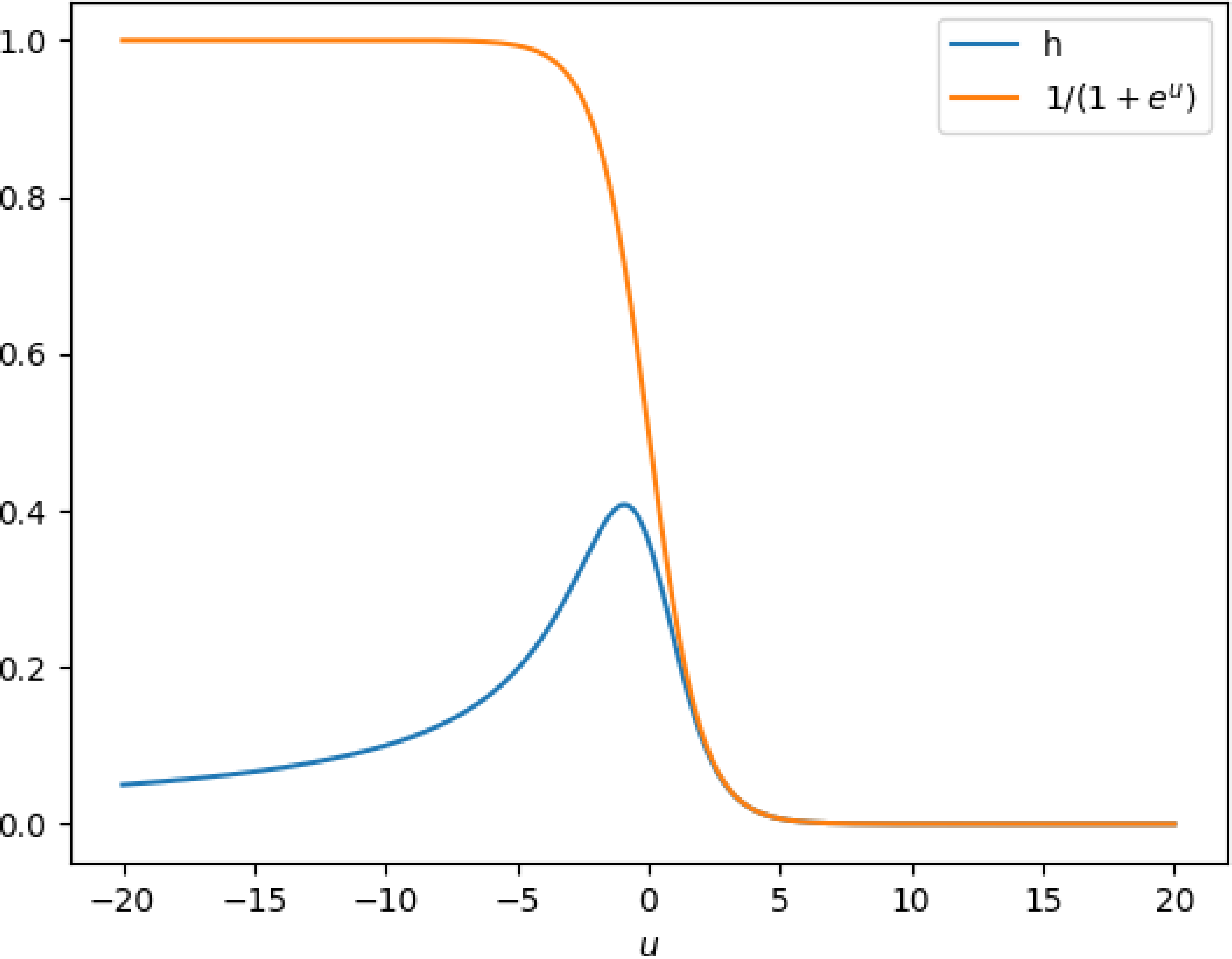
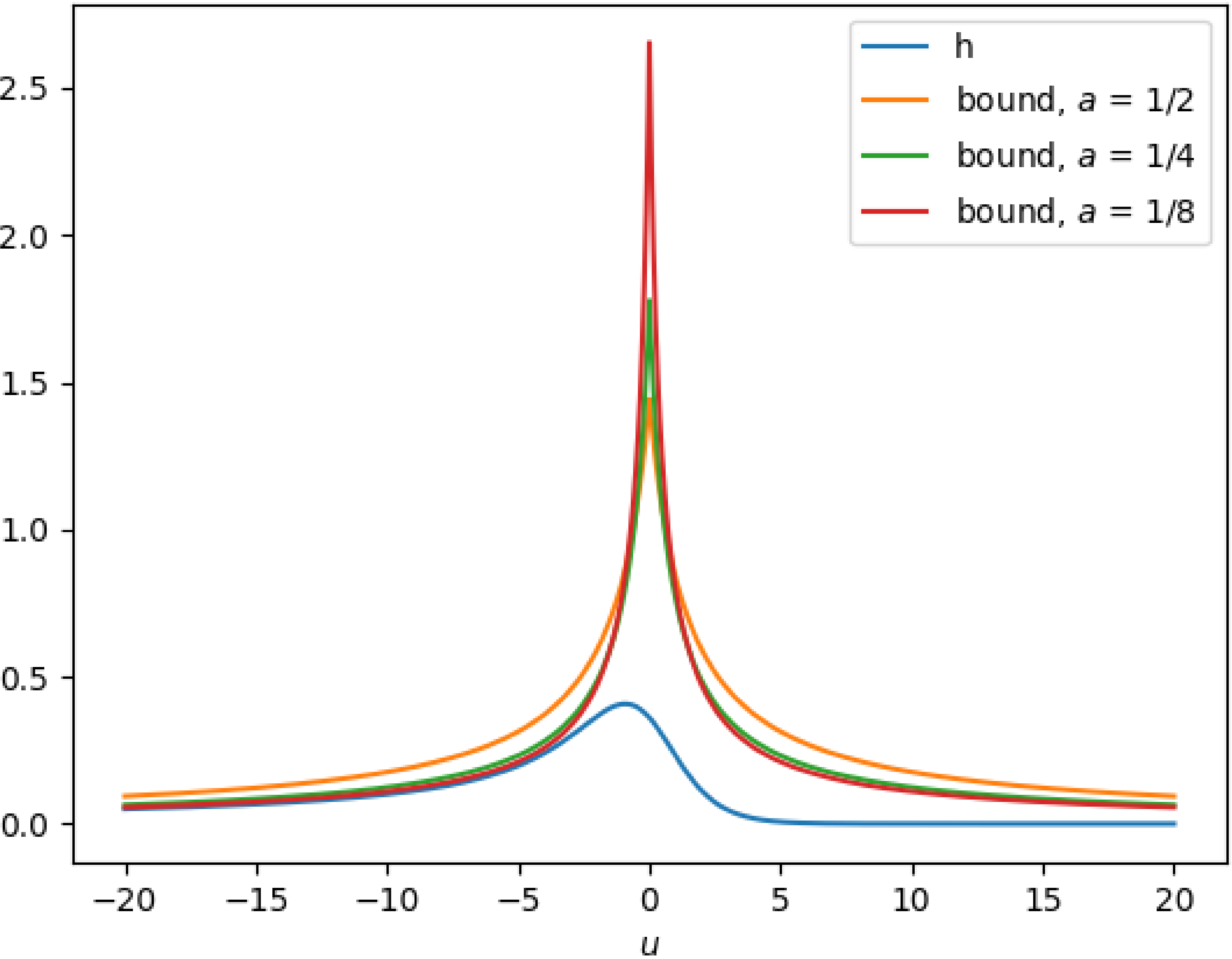
Figure 5: Upper bounds for function $h$ defined in (23): (left) bound of Lemma A.5, (right) bounds of Lemma A.6.

Lemma A.6

Function $h$, defined in (23), satisifies, for every fixed $a\in(0,1/2]$,

$$h(u)\leq\frac{1}{H(a)+(1-a)|u|}\hbox{ for all }u\in\mathbb{R}$$ (25)

where $H(a)=a\log(1/a)+(1-a)\log(1/(1-a))$. Furthermore, $h(u)\sim 1/|u|$ as $u$ tends to $-\infty$.

By Lemma A.6, it follows that condition of Lemma 3.12 is satisfied by uncertainty sampling according to

$$\pi^{*}(u)=\frac{\beta}{2(1-c)}\min\left\{\rho R^{2}\frac{1}{H(a)+(1-a)|u|},1\right\}.$$

A.13.1 Proof of Lemma A.5

We need to prove that for every $u\in\mathbb{R}$,

$$(1+e^{u})^{2}\log(1+e^{-u})\geq 1+e^{u}.$$

By dividing both sides in the last inequality with $(1+e^{u})^{2}$ and the fact $1/(1+e^{u})=1-1/(1+e^{-u})$, we note that the last above inequality is equivalent to

$$\log(1+e^{-u})\geq 1-\frac{1}{1+e^{-u}}.$$

By straightforward calculus, this can be rewritten as

$$\log\left(1-\left(1-\frac{1}{1+e^{-u}}\right)\right)\leq-\left(1-\frac{1}{1+e^{-u}}\right).$$

This clearly holds true because $1-1/(1+e^{-u})\in(0,1)$ and $\log(1-z)\leq-z$ for every $z\in(0,1)$.

It remains only to show that $\lim_{u\rightarrow\infty}h(u)/(1-\sigma(u))=1$. This is clearly true as

$$\frac{h(u)}{1-\sigma(u)}=\frac{1}{(1+e^{u})\log(1+e^{-u})}$$

which goes to $1$ as $u$ goes to infinity.

A.14 Proof of Lemma A.6

We first consider the case $u\leq 0$. Fix an arbitrary $v\leq 0$. Since $u\mapsto\log(1+e^{u})$ is a convex function it is lower bounded by the tangent passing through $v$, i.e.

$$\log(1+e^{-u})\geq\log(1+e^{-v})-\frac{1}{1+e^{v}}(u-v).$$

Now, let $a$ be such that $1-a=1/(1+e^{v})$. Since $v\leq 0$, we have $a\in(0,1/2]$. It follows that for any fixed $a\in(0,1/2]$,

$$\log(1+e^{-u})\geq H(a)-(1-a)u.$$

Using this along with the obvious fact $(1+e^{u})^{2}\geq 1$, we have that for every $u\leq 0$,

$$h(u)\leq\frac{1}{\log(1+e^{-u})}\leq\frac{1}{H(a)+(1-a)|u|}.$$

We next consider the case $u\geq 0$. It sufficies to show that for every $u\geq 0$, $h(u)\leq h(-u)$, and hence the upper bound established for the previous case applies. The condition $h(u)\leq h(-u)$ is equivalent to

$$\frac{1}{(1+e^{u})^{2}\log(1+e^{-u})}\leq\frac{1}{(1+e^{-u})^{2}\log(1+e^{u})}.$$

By straightforward calculus, this is equivalent to

$$f(u):=(1-e^{-2u})\log(1+e^{u})-u\geq 0.$$

This holds because function (i) $f$ is increasing on $[0,u_{0}]$ and decreasing on $[u_{0},\infty)$, for some $u_{0}\geq 0$, (ii) $f(0)=0$ and (iii) $\lim_{u\rightarrow\infty}f(u)=0$. Properties (ii) and (iii) are easy to check. We only show that property (i) holds true. By straightforward calculus,

$$f^{\prime}(u)=e^{-2u}(2\log(1+e^{u})-e^{u}).$$

It suffices to show that there is a unique $u^{*}\in\mathbb{R}$ such that $f^{\prime}(u^{*})=0$. For any such $u^{*}$ it must hold $2\log(1+e^{u^{*}})-e^{u^{*}}$. Let $v=e^{v^{*}}$. Then, $2\log(1+v)=v$, which is equivalent to

$$1+v=e^{\frac{v}{2}}.$$

Both sides of the last equation are increasing in $v$, and the left-hand side is larger than the right-hand side for $v=1$. Since the right-hand side is larger than the left-hand side for any large enough $v$, it follows that there is a unique point $v$ at which the sides of the equation are equal. This shows that there is a unique $u^{*}\geq 0$ such that $f^{\prime}(u^{*})=0$.

It remains to show that $\lim_{u\rightarrow-\infty}h(u)/(1/|u|)=1$, i.e.

$$\lim_{u\rightarrow-\infty}\frac{-u}{(1+e^{u})^{2}\log(1+e^{-u})}=1$$

which clearly holds true as both $1/(1+e^{u})^{2}$ and $-u/\log(1+e^{-u})$ go to $1$ as $u$ goes to $-\infty$.

A.15 Polyak’s step size for multi-class classification

We consider multi-class classification according to prediction function

$$p(y\mid x,\theta)=\frac{e^{x^{\top}\theta_{y}}}{\sum_{y^{\prime}\in\mathcal{Y}}e^{x^{\top}\theta_{y^{\prime}}}},\hbox{ for }y\in\mathcal{Y}.$$

Assume that $\ell$ is the cross-entropy function. Let

$$u(x,y,\theta)=-\log\left(\sum_{y^{\prime}\in\mathcal{Y}\setminus\{y\}}e^{-(x^{\top}\theta_{y}-x^{\top}\theta_{y^{\prime}})}\right).$$

It can be shown that

$$\frac{||\nabla_{\theta}\ell(x,y,\theta)||^{2}}{\ell(x,y,\theta)}\leq 2||x||^{2}h(u(x,y,\theta))$$

where function $h$ is defined in (23). Hence, condition of Lemma 3.12 holds under

$$\pi(u)\geq\frac{\beta}{2(1-c)}\min\left\{2\rho R^{2}h(u),1\right\}.$$

For given $\theta$ and $x$, let $\theta_{(1)},\ldots,\theta_{(k)}$ be an ordering of $\theta_{1},\ldots,\theta_{k}$ such that $x^{\top}\theta_{(1)}\geq\cdots\geq x^{\top}\theta_{(k)}$. Sampling according to function $\pi^{*}$ of the gap $g=|x^{\top}\theta_{(1)}-x^{\top}\theta_{(k)}|$,

$$\pi^{*}(g)=\frac{\beta}{2(1-c)}\min\left\{2\rho R^{2}h^{*}(g),1\right\},$$

where

$$h^{*}(g)=\frac{1}{H(a)+(1-a)\max\{g-\log(k-1),0\}},$$

satisfies condition of Lemma 3.12.

We next provide proofs for assertions made above. The loss function is assumed to be the cross-entropy loss function, i.e.

$$\ell(x,y,\theta)=-\log\left(\frac{e^{x^{\top}\theta_{y}}}{\sum_{y^{\prime}\in\mathcal{Y}}e^{x^{\top}\theta_{y^{\prime}}}}\right).$$

Note that we can write

$$\ell(x,y,\theta)=-\left(\phi(x,y)^{\top}\theta-\log\left(\sum_{y^{\prime}\in\mathcal{Y}\setminus\{y\}}e^{\phi(x,y^{\prime})^{\top}\theta}\right)\right).$$

We consider

$$\frac{||\nabla_{\theta}\ell(x,y,\theta)||^{2}}{\ell(x,y,\theta)}$$

which is plays a key role in the condition of Lemma 3.12.

It holds

$$\nabla_{\theta}\ell(x,y,\theta)=-\left(\phi(x,y)-\frac{\sum_{y^{\prime}\in\mathcal{Y}\setminus\{y\}}e^{\phi(x,y^{\prime})^{\top}\theta}\phi(x,y^{\prime})}{\sum_{y^{\prime}\in\mathcal{Y}\setminus\{y\}}e^{\phi(x,y^{\prime})^{\top}\theta}}\right)$$

and

$$||\nabla_{\theta}\ell(x,y,\theta)||^{2} = \left(1-\frac{e^{\phi(x,y)^{\top}\theta}}{\sum_{z\in\mathcal{Y}\setminus\{y\}}e^{\phi(x,z)^{\top}\theta}}\right)^{2}||x||^{2}+\sum_{y^{\prime}\in\mathcal{Y}\setminus\{y\}}\left(\frac{e^{\phi(x,y^{\prime})^{\top}\theta}}{\sum_{z\in\mathcal{Y}\setminus\{y\}}e^{\phi(x,z)^{\top}\theta}}\right)^{2}||x||^{2}$$

$$= \left(\left(1-e^{-\ell(x,y,\theta)}\right)^{2}+\sum_{y^{\prime}\in\mathcal{Y}\setminus\{y\}}\left(e^{-\ell(x,y^{\prime},\theta)}\right)^{2}\right)||x||^{2}.$$

From the last equation, it follows

$$||x||^{2}\left(1-e^{-\ell(x,y,\theta)}\right)^{2}\leq||\nabla_{\theta}\ell(x,y,\theta)||^{2}\leq 2||x||^{2}\left(1-e^{-\ell(x,y,\theta)}\right)^{2}.$$

Note that $\ell(x,y,\theta)=\log(1+e^{-u(x,y,\theta)})$ where

$$u(x,y,\theta)=-\log\left(\sum_{y^{\prime}\in\mathcal{Y}\setminus\{y\}}e^{-(x^{\top}\theta_{y}-x^{\top}\theta_{y^{\prime}})}\right).$$

It follows

$$||x||^{2}h(u(x,y,\theta))\leq\frac{||\nabla_{\theta}\ell(x,y,\theta)||^{2}}{\ell(x,y,\theta)}\leq 2||x||^{2}h(u(x,y,\theta))$$

where $h$ is function defined in (23).

The following equation holds

$$u(x,y,\theta)=\theta_{y}^{\top}x-\max_{z\in\mathcal{Y}\setminus\{y\}}x^{\top}\theta_{z}-\log\left(\sum_{y^{\prime}\in\mathcal{Y}\setminus\{y\}}e^{-(\max_{z\in\mathcal{Y}\setminus\{y\}}x^{\top}\theta_{z}-x^{\top}\theta_{y^{\prime}})}\right).$$

Note that

$$|u(x,y,\theta)| \geq |x^{\top}\theta_{y}-\max_{z\in\mathcal{Y}\setminus\{y\}}x^{\top}\theta_{z}|-\log\left(\sum_{y^{\prime}\in\mathcal{Y}\setminus\{y\}}e^{-(\max_{z\in\mathcal{Y}\setminus\{y\}}x^{\top}\theta_{z}-x^{\top}\theta_{y^{\prime}})}\right)$$

$$\geq |x^{\top}\theta_{(1)}-x^{\top}\theta_{(2)}|-\log(k-1).$$

Combining with Lemma A.6, for every $a\in(0,1/2]$,

$$h(u(x,y,\theta))\leq\frac{1}{H(a)+(1-a)|u|}\leq h^{*}(|x^{\top}\theta_{(1)}-x^{\top}\theta_{(2)}|)$$

where

$$h^{*}(g)=\left\{\begin{array}[]{ll}\frac{1}{H(a)}&\hbox{ if }g\leq\log(k-1)\\ \frac{1}{H(a)-(1-a)\log(k-1)+(1-a)g}&\hbox{ if }g>\log(k-1).\end{array}\right.$$

A.16 Further details on experimental setup

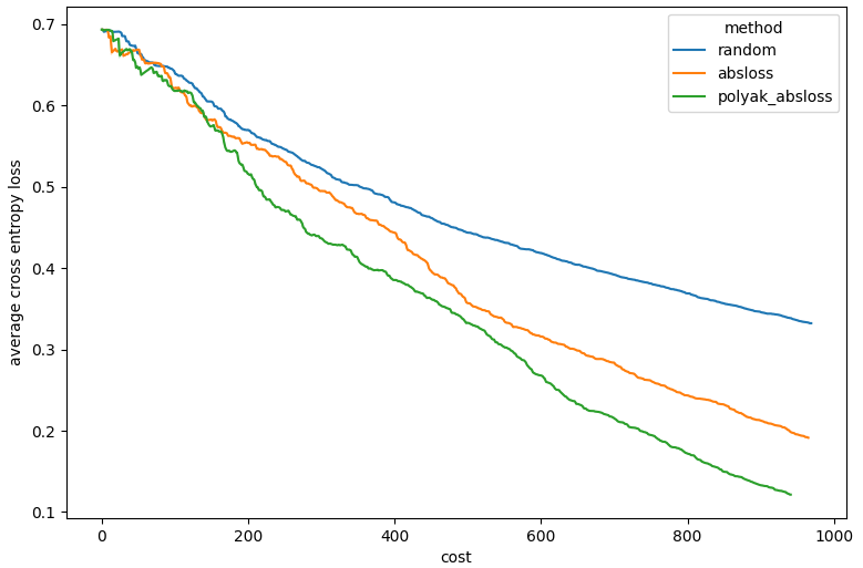
Figure 6: Average cross entropy loss as a function of labeling cost for different sampling methods.

A.16.1 Hyperparameter tuning

We used the Tree-structured Parzen Estimator (TPE) (Bergstra et al., 2011) algorithm in the hyperopt package (Bergstra et al., 2013) to tune the relevant hyperparameters for each method and minimise the average progressive cross entropy loss. For Polyak absloss and Polyak exponent we set the search space of $\eta$ to $[0.01,1]$ and the search space of $\rho$ to $[0,1]$. Note that the values of $\eta$ and $\rho$ influence the rate of sampling. In line with the typical goal of active learning, we aim to learn efficiently and minimise loss under some desired rate of sampling. Therefore, for every configuration of $\eta$ and $\rho$ we use binary search to find the value of $\beta$ that achieves some target empirical sampling rate. Observe that if we would not control for $\beta$, then our hyperparameter tuning setup would simply find values of $\eta$ and $\rho$ that lead to very high sampling rates, which is not in line with the goal of active learning. In the hyperparameter tuning we set the target empirical sampling rate to 50%.

A.16.2 Related to Figure 2

We similarly used binary search to find the value of $\beta$ that correspondingly achieves the two target values 1% and 10% with Polyak power function, while using the values of $\eta$ and $\rho$ that were optimised for a sampling rate of 50%. Therefore, our findings of the gains achieved for selective sampling according to stochastic Polyak’s step size are likely conservative since $\eta$ and $\rho$ were not optimised for specifically these sampling rates.

A.16.3 Related to Figures 3 and 4

We compare Polyak absolute loss sampling to absolute loss sampling and random sampling. In this setting we have no control over the sampling rate of absolute loss sampling. Hence, we first run absolute loss sampling to find an empircal sampling rate of 14.9%. We then again use binary search to find the value of $\beta$ to match this sampling rate with Polyak absolute loss sampling. Again, this setup is conservative with respect to the gains of Polyak absolute loss sampling as $\eta$ and $\rho$ were optimised for a sampling rate of 50%.

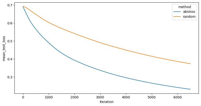
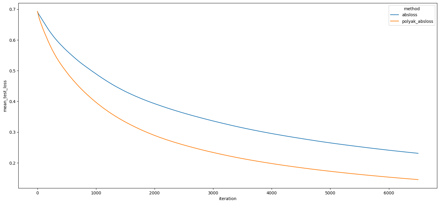
Figure 7: Average cross entropy loss on a hold-out testing set for different sampling methods.

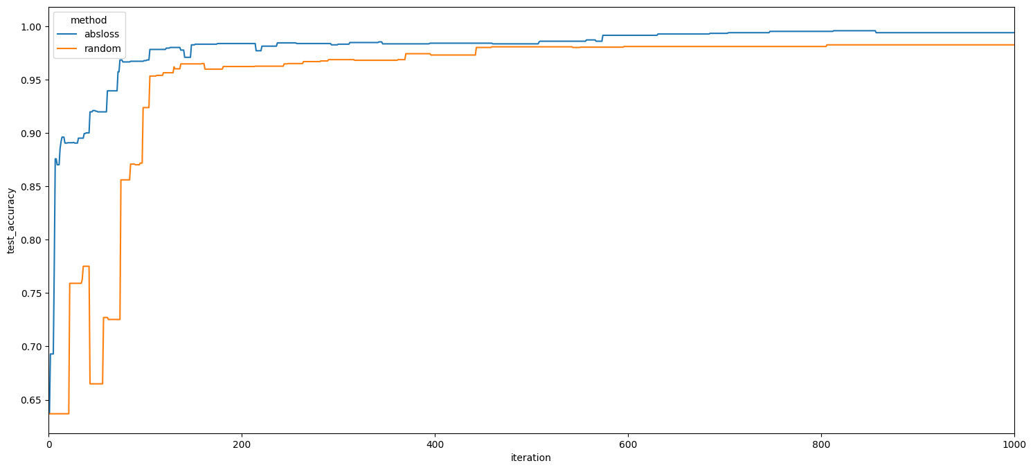
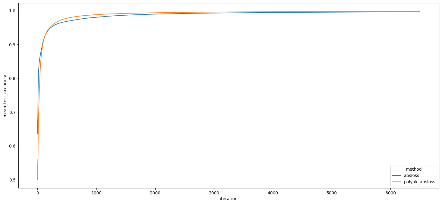
Figure 8: Test accuracy for different sampling methods.

A.17 Additional numerical results

Below are some additional empirical experiments conducted on the same mushroom classification dataset (Chang and Lin, 2011) described in Section 4. The training loss as a function of the number of labeled instances that were selected for training (i.e., cost) is presented in Figure 6. Performance of different sampling methods on the hold-out testing set is presented in Figure 7 (average test loss) and Figure 8 (test accuracy). As can be seen from the figures, the relative performance of different sampling methods is consistent across different metrics.

We will make the code and the dataset from our numerical experiments available for download in the final version of the manuscript.

References

- Agarwal (2013) Alekh Agarwal. Selective sampling algorithms for cost-sensitive multiclass prediction. In Sanjoy Dasgupta and David McAllester, editors, Proceedings of the 30th International Conference on Machine Learning, volume 28 of Proceedings of Machine Learning Research, pages 1220–1228, Atlanta, Georgia, USA, 17–19 Jun 2013. PMLR.
- Bergstra et al. (2011) James Bergstra, Rémi Bardenet, Yoshua Bengio, and Balázs Kégl. Algorithms for hyper-parameter optimization. Advances in Neural Information Processing Systems, 24, 2011.
- Bergstra et al. (2013) James Bergstra, Daniel Yamins, and David Cox. Making a science of model search: Hyperparameter optimization in hundreds of dimensions for vision architectures. In Proceedings of the 30th International Conference on Machine Learning, pages 115–123. PMLR, 2013.
- Blum et al. (1999) Avrim Blum, Adam Kalai, and John Langford. Beating the hold-out: Bounds for k-fold and progressive cross-validation. In Proceedings of the Twelfth Annual Conference on Computational Learning Theory (COLT), pages 203–208, 1999.
- Bubeck (2015) Sébastien Bubeck. Convex optimization: Algorithms and complexity. Found. Trends Mach. Learn., 8(3–4):231–357, nov 2015.
- Cavallanti et al. (2011) Giovanni Cavallanti, Nicolò Cesa-Bianchi, and Claudio Gentile. Learning noisy linear classifiers via adaptive and selective sampling. Machine Learning, 83(1):71–102, 2011.
- Cesa-Bianchi et al. (2006) Nicoló Cesa-Bianchi, Claudio Gentile, and Luca Zaniboni. Worst-case analysis of selective sampling for linear classification. Journal of Machine Learning Research, 7(44):1205–1230, 2006.
- Cesa-Bianchi et al. (2009) Nicolò Cesa-Bianchi, Claudio Gentile, and Francesco Orabona. Robust bounds for classification via selective sampling. In Proceedings of the 26th Annual International Conference on Machine Learning, ICML ’09, page 121–128, New York, NY, USA, 2009. Association for Computing Machinery.
- Chang and Lin (2011) Chih-Chung Chang and Chih-Jen Lin. Libsvm: a library for support vector machines. ACM transactions on intelligent systems and technology (TIST), 2(3):1–27, 2011.
- Crammer and Singer (2002) Koby Crammer and Yoram Singer. On the algorithmic implementation of multiclass kernel-based vector machines. J. Mach. Learn. Res., 2:265–292, mar 2002. ISSN 1532-4435.
- Dasgupta et al. (2009) Sanjoy Dasgupta, Adam Tauman Kalai, and Claire Monteleoni. Analysis of perceptron-based active learning. Journal of Machine Learning Research, 10(11):281–299, 2009.
- Dekel et al. (2012) Ofer Dekel, Claudio Gentile, and Karthik Sridharan. Selective sampling and active learning from single and multiple teachers. J. Mach. Learn. Res., 13(1):2655–2697, sep 2012. ISSN 1532-4435.
- Freund et al. (1997) Yoav Freund, H. Sebastian Seung, Eli Shamir, and Naftali Tishby. Selective sampling using the query by committee algorithm. Machine Learning, 28(2):133–168, 1997.
- Gilad-bachrach et al. (2005) Ran Gilad-bachrach, Amir Navot, and Naftali Tishby. Query by committee made real. In Y. Weiss, B. Schölkopf, and J. Platt, editors, Advances in Neural Information Processing Systems, volume 18. MIT Press, 2005.
- Kirsch and Gal (2022) Andreas Kirsch and Yarin Gal. Unifying approaches in active learning and active sampling via fisher information and information-theoretic quanties. Transactions on Machine Learning Research, 2022.
- Kirsch et al. (2019) Andreas Kirsch, Joost van Amersfoort, and Yarin Gal. Batchbald: Efficient and diverse batch acquisition for deep bayesian active learning. In H. Wallach, H. Larochelle, A. Beygelzimer, F. d'Alché-Buc, E. Fox, and R. Garnett, editors, Advances in Neural Information Processing Systems, volume 32. Curran Associates, Inc., 2019.
- Lahlou et al. (2022) Salem Lahlou, Moksh Jain, Hadi Nekoei, Victor I Butoi, Paul Bertin, Jarrid Rector-Brooks, Maksym Korablyov, and Yoshua Bengio. Deup: Direct epistemic uncertainty prediction. Transactions on Machine Learning Research, 2022.
- Lewis and Gale (1994) David D. Lewis and William A. Gale. A sequential algorithm for training text classifiers. In Bruce W. Croft and C. J. van Rijsbergen, editors, SIGIR ’94, pages 3–12, London, 1994. Springer London.
- Liu and Li (2023) Shang Liu and Xiaocheng Li. Understanding uncertainty sampling, 2023. URL https://arxiv.org/abs/2307.02719.
- Loizou et al. (2021) Nicolas Loizou, Sharan Vaswani, Issam Hadj Laradji, and Simon Lacoste-Julien. Stochastic Polyak step-size for SGD: An adaptive learning rate for fast convergence. In Arindam Banerjee and Kenji Fukumizu, editors, Proceedings of The 24th International Conference on Artificial Intelligence and Statistics, volume 130 of Proceedings of Machine Learning Research, pages 1306–1314. PMLR, 13–15 Apr 2021.
- Lughofer and Pratama (2018) Edwin Lughofer and Mahardhika Pratama. Online active learning in data stream regression using uncertainty sampling based on evolving generalized fuzzy models. IEEE Transactions on Fuzzy Systems, 26(1):292–309, 2018.
- Luo et al. (2021) Jian Luo, Jianzong Wang, Ning Cheng, and Jing Xiao. Loss prediction: End-to-end active learning approach for speech recognition. In 2021 International Joint Conference on Neural Networks (IJCNN), pages 1–7. IEEE, 2021.
- Mussmann and Liang (2018) Stephen Mussmann and Percy S Liang. Uncertainty sampling is preconditioned stochastic gradient descent on zero-one loss. In S. Bengio, H. Wallach, H. Larochelle, K. Grauman, N. Cesa-Bianchi, and R. Garnett, editors, Advances in Neural Information Processing Systems, volume 31. Curran Associates, Inc., 2018.
- Nguyen et al. (2021) Minh-Tien Nguyen, Guido Zuccon, Gianluca Demartini, et al. Loss-based active learning for named entity recognition. In 2021 International Joint Conference on Neural Networks (IJCNN), pages 1–8. IEEE, 2021.
- Nguyen et al. (2022) Vu-Linh Nguyen, Mohammad Hossein Shaker, and Eyke Hüllermeier. How to measure uncertainty in uncertainty sampling for active learning. Machine Learning, 111(1):89–122, 2022.
- Orabona and Cesa-Bianchi (2011) Francesco Orabona and Nicolò Cesa-Bianchi. Better algorithms for selective sampling. In Proceedings of the 28th International Conference on International Conference on Machine Learning, ICML’11, page 433–440, Madison, WI, USA, 2011. Omnipress. ISBN 9781450306195.
- Raj and Bach (2022) Anant Raj and Francis Bach. Convergence of uncertainty sampling for active learning. In Kamalika Chaudhuri, Stefanie Jegelka, Le Song, Csaba Szepesvari, Gang Niu, and Sivan Sabato, editors, Proceedings of the 39th International Conference on Machine Learning, volume 162 of Proceedings of Machine Learning Research, pages 18310–18331. PMLR, 17–23 Jul 2022.
- Rennie (2005) Jason Rennie. Smooth hinge classification, 2005. URL http://qwone.com/ jason/writing/smoothHinge.pdf.
- Rennie and Srebro (2005) Jason Rennie and Nathan Srebro. Loss functions for preference levels: Regression with discrete ordered labels. Proceedings of the IJCAI Multidisciplinary Workshop on Advances in Preference Handling, 01 2005.
- Rosenblatt (1958) F. Rosenblatt. he perceptron: a probabilistic model for information storage and organization in the brain. Psychological review, 65(6):386–408, 1958.
- Roy and McCallum (2001) Nicholas Roy and Andrew McCallum. Toward optimal active learning through sampling estimation of error reduction. In Proceedings of the Eighteenth International Conference on Machine Learning, page 441–448, San Francisco, CA, USA, 2001. Morgan Kaufmann Publishers Inc.
- Schohn and Cohn (2000) Greg Schohn and David Cohn. Less is more: Active learning with support vector machines. In Proceedings of the Seventeenth International Conference on Machine Learning, ICML ’00, page 839–846, San Francisco, CA, USA, 2000. Morgan Kaufmann Publishers Inc.
- Settles (2012) Burr Settles. Active learning: Synthesis lectures on artificial intelligence and machine learning. Springer Cham, 2012.
- Settles et al. (2007) Burr Settles, Mark Craven, and Soumya Ray. Multiple-instance active learning. In J. Platt, D. Koller, Y. Singer, and S. Roweis, editors, Advances in Neural Information Processing Systems, volume 20. Curran Associates, Inc., 2007.
- Seung et al. (1992) H. S. Seung, M. Opper, and H. Sompolinsky. Query by committee. COLT ’92, page 287–294, New York, NY, USA, 1992. Association for Computing Machinery. ISBN 089791497X.
- Shen (2021) Jie Shen. On the power of localized perceptron for label-optimal learning of halfspaces with adversarial noise. In Marina Meila and Tong Zhang, editors, Proceedings of the 38th International Conference on Machine Learning, volume 139 of Proceedings of Machine Learning Research, pages 9503–9514, 18–24 Jul 2021.
- Wang et al. (2016) Ran Wang, Chi-Yin Chow, and Sam Kwong. Ambiguity-based multiclass active learning. IEEE Transactions on Fuzzy Systems, 24(1):242–248, 2016.
- Yan and Zhang (2017) Songbai Yan and Chicheng Zhang. Revisiting perceptron: Efficient and label-optimal learning of halfspaces. In I. Guyon, U. Von Luxburg, S. Bengio, H. Wallach, R. Fergus, S. Vishwanathan, and R. Garnett, editors, Advances in Neural Information Processing Systems, volume 30. Curran Associates, Inc., 2017.
- Yang and Loog (2016) Y. Yang and M. Loog. Active learning using uncertainty information. In Proceedings of the International Conference on Pattern Recoginition (ICPR), page 2646–2651, 2016.
- Yang et al. (2015) Yi Yang, Zhigang Ma, Feiping Nie, Xiaojun Chang, and Alexander G. Hauptmann. Multi-class active learning by uncertainty sampling with diversity maximization. International Journal of Computer Vision, 113(2):113–127, 2015.
- Yoo and Kweon (2019) Donggeun Yoo and In So Kweon. Learning loss for active learning. In Proceedings of the IEEE/CVF Conference on Computer Vision and Pattern Recognition (CVPR), June 2019.
- Zhu et al. (2010) Jingbo Zhu, Huizhen Wang, Benjamin K. Tsou, and Matthew Ma. Active learning with sampling by uncertainty and density for data annotations. IEEE Transactions on Audio, Speech, and Language Processing, 18(6):1323–1331, 2010.