Solving Long-run Average Reward Robust MDPs via Stochastic Games

Abstract

Markov decision processes (MDPs) provide a standard framework for sequential decision making under uncertainty. However, transition probabilities in MDPs are often estimated from data and MDPs do not take data uncertainty into account. Robust Markov decision processes (RMDPs) address this shortcoming of MDPs by assigning to each transition an uncertainty set rather than a single probability value. The goal of solving RMDPs is then to find a policy which maximizes the worst-case performance over the uncertainty sets. In this work, we consider polytopic RMDPs in which all uncertainty sets are polytopes and study the problem of solving long-run average reward polytopic RMDPs. Our focus is on computational complexity aspects and efficient algorithms. We present a novel perspective on this problem and show that it can be reduced to solving long-run average reward turn-based stochastic games with finite state and action spaces. This reduction allows us to derive several important consequences that were hitherto not known to hold for polytopic RMDPs. First, we derive new computational complexity bounds for solving long-run average reward polytopic RMDPs, showing for the first time that the threshold decision problem for them is in $\textsc{NP}\cap\textsc{coNP}$ and that they admit a randomized algorithm with sub-exponential expected runtime. Second, we present Robust Polytopic Policy Iteration (RPPI), a novel policy iteration algorithm for solving long-run average reward polytopic RMDPs. Our experimental evaluation shows that RPPI is much more efficient in solving long-run average reward polytopic RMDPs compared to state-of-the-art methods based on value iteration.

1 Introduction

Robust Markov decision processes

Markov decision processes (MDPs) are widely adopted as a framework for sequential decision making in environments that exhibit stochastic uncertainty Puterman (1994). The goal of solving an MDP is to compute a policy which maximizes expected payoff with respect to some reward objective. However, classical algorithms for solving MDPs assume that transition probabilities are known and available. While this is plausible from a theoretical perspective, in practice this assumption is not always justified – transition probabilities are typically inferred from data and as such their estimates come with a certain level of uncertainty. This has motivated the study of robust Markov decision processes (RMDPs) Nilim and Ghaoui (2003); Iyengar (2005). RMDPs differ from MDPs in that they only assume knowledge of some uncertainty set containing true transition probabilities. The goal of solving RMDPs is to compute a policy which maximizes the worst-case expected payoff with respect to all possible choices of transition probabilities belonging to the uncertainty set. The advantage of considering RMDPs rather than MDPs for planning and sequential decision making tasks is that solving RMDPs provides policies that are robust to potential uncertainty in the underlying environment model.

Long-run average reward RMDPs

Recent years have seen significant interest in solving RMDPs. Two most fundamental reward objectives defined over unbounded or infinite time horizon trajectories are the discounted-sum reward and the long-run average reward. While there are many works on solving discounted-sum reward RMDPs (see an overview of related work below), the problem of solving long-run average reward RMDPs remains comparatively less explored. However, long-run average reward is, along with discounted-sum, one of the two fundamental objectives used in agent planning and reinforcement learning Puterman (1994); Sutton et al. (1999). Unlike discounted-sum, which places more emphasis on earlier rewards, long run average reward focuses on the long-term sustainability of the reward signal.

Prior work and challenges

Most prior work on solving long-run average reward RMDPs focuses on special instances of RMDPs in which uncertainty sets are either products of intervals (i.e. $L^{\infty}$-balls) or $L^{1}$-balls around some pivot probability distribution. These works typically focus on studying Blackwell optimality in RMDPs. In standard MDPs, Blackwell optimality Puterman (1994) is a classical result which says that there exists some threshold discount factor $\gamma^{\ast}\in[0,1)$ such that the same policy maximizes expected discounted-sum reward for any discount factor $\gamma\in[\gamma^{*},1)$ while also maximizing the long-run average reward in the MDP. This allows using the methods for discounted-sum reward MPDs to solve long-run average reward MDPs.

The work of Tewari and Bartlett (2007) considers RMDPs in which uncertainty sets are products of intervals (also called interval MDPs Givan et al. (2000)), and is the first to establish Blackwell optimality for interval MDPs. It also proposes a value iteration algorithm for solving long-run average reward interval MDPs. The works Grand-Clément and Petrik (2023); Goyal and Grand-Clément (2023) establish Blackwell optimality for RMDPs with general polytopic uncertainty sets. Moreover, the work Grand-Clément and Petrik (2023) designs value and policy iteration algorithms for solving long-run average reward RMDPs with interval or $L^{1}$-uncertainty sets. Finally, the recent work of Wang et al. (2023) establishes Blackwell optimality and proposes a value iteration algorithm for a general class of RMDPs in which uncertainty sets are only assumed to be compact, but in which the RMDP is assumed to be unichain.

While these works present significant advances in solving long-run average reward RMDPs, our understanding of this problem still suffers from a few limitations:

• Computational complexity. While prior works focus on studying Blackwell optimality in RMDPs and algorithms for solving them, no upper bound on the computational complexity of solving this problem is known.

• Structural or uncertainty restrictions. The value iteration algorithm of Wang et al. (2023) requires the RMDP to be unichain. On the other hand, other algorithms discussed above are applicable to RMDPs with either interval or $L^{1}$-uncertainty sets.

• Policy iteration. Both in classical MDP Puterman (1994) and in discounted-sum RMDP Ho et al. (2021) literature, policy iteration is known to be more efficient than value iteration. However, for RMDPs with uncertainty sets that are not intervals or $L^{1}$-balls, the only available algorithm is that of Wang et al. (2023) which is based on value iteration.

Our contributions

This work focuses on computational complexity aspects and efficient algorithms for solving long-run average reward RMDPs and our goal is to address the limitations discussed above. To that end, we consider polytopic RMDPs in which all uncertainty sets are assumed to be polytopes and which unify and strictly subsume RMDPs with interval or $L^{1}$-uncertainty sets. We present a new perspective on the problem of solving long-run average reward polytopic RMDPs by showing that it admits a polynomial-time reduction to the problem of solving long-run average reward turn-based stochastic games (TBSGs) in which both state and action sets are finite. While the connection between RMDPs and TBSGs has been informally mentioned in several prior works, e.g. Goyal and Grand-Clément (2023), we are not aware that any prior work has actually formalized this reduction. The reduction formalization turns out to be technically non-trivial and we provide a first formal proof of the correctness of the reduction. The reduction formalization is the main technical contribution of our work.

While definitely compelling, the reduction is not only of theoretical interest. TBSGs have been widely studied within computational game theory and formal methods communities Shapley (1953); Filar and Vrieze (1996); Kučera (2011) and this reduction allows us to leverage a plethora of results on TBSGs in order to establish new results on long-run average reward RMDPs that were hitherto not know to be true. In particular, our results allow us to overcome all the limitations discussed above. Our main contributions are as follows:

1. We establish novel complexity results on solving long-run average reward polytopic RMDPs, showing for the first time that the threshold decision problem for them is in $\textsc{NP}\cap\textsc{coNP}$ and that they admit a randomized algorithm with sub-exponential expected runtime.

2. By utilizing Blackwell optimality for TBSGs and the fact that policy iteration has already been shown to be sound for discounted-sum reward TBSGs, we propose Robust Polytopic Policy Iteration (RPPI), our novel algorithm for solving long-run average reward polytopic RMDPs. Our algorithm does not impose structural restrictions on the RMDP such as unichain or aperiodic.

3. Experimental evaluation. We implement RPPI and experimentally compare it against the value iteration algorithm of Wang et al. (2023). We show that RPPI achieves significant efficiency gains on unichain RMDPs while also being practically applicable to RMDPs without such structural restrictions.

Related work

The related work on solving long-run average reward RMDPs was discussed above, hence we omit repetition. In what follows, we overview a larger body of existing works on solving discounted-sum reward RMDPs. Existing approaches can be classified into model-based and model-free. Model-based approaches assume the full knowledge of the uncertainty set and compute optimal policies with exact values on the worst-case expected payoff that they achieve, see e.g. Nilim and Ghaoui (2003); Iyengar (2005); Wiesemann et al. (2013); Kaufman and Schaefer (2013); Tamar et al. (2014); Ghavamzadeh et al. (2016); Ho et al. (2021). These works also provide deep theoretical insight into RMDPs and show that many classical results on MDPs transfer to the RMDP setting. Model-free approaches, on the other hand, do not assume the full knowledge of the uncertainty set. Rather, they learn the uncertainty sets from data and as such provide more scalable and practical algorithms, although without guarantees on optimality of learned policies Roy et al. (2017); Tessler et al. (2019); Wang and Zou (2021, 2022); Ho et al. (2018); Yang et al. (2022).

In the final days of preparing this submission, we found a concurrent work of Grand-Clement et al. (2023) which also explores the connection between long-run average reward RMDPs and TBSGs in order to study Blackwell optimality. Our focus in this work is on computational complexity aspects and efficient algorithms for solving this problem. Furthermore, we also establish that our reduction is efficient, along with its formal correctness, that allows transfer of algorithms from the stochastic games literature to RMDPs.

2 Preliminaries and Models

For a set $X$, we denote by $\Delta(X)$ the set of all probability distributions over $X$. We use $\textsc{Pow}(X)$ to denote the set of all subsets of $X$. For two sets $X$ and $Y$, we denote by $Y^{X}$ the set of all functions with domain $X$ and co-domain $Y$.

2.1 Robust MDPs and Problem Statement

MDPs

A (finite-state, discrete-time) Markov decision process (MDP) Puterman (1994) is a tuple $(S,A,\delta,r,s_{0})$, where

• $S$ is a finite set of states;

• $A$ is a finite set of actions;

• $\delta\colon S\times A\rightarrow\Delta(S)$ is a probabilistic transition function;

• $r\colon S\times A\rightarrow\mathbb{R}$ is a reward function,

• $s_{0}\in S$ is the initial state.

We abbreviate the transition probability $\delta(s,a)(s^{\prime})$ from $s$ to $s^{\prime}$ under action $a$ by $\delta(s^{\prime}\mid s,a)$.

The dynamics of an MDP are defined through the notion of a policy. A policy is a map $\sigma:(S\times A)^{\ast}\times S\rightarrow\Delta(A)$ which to each finite history of state-action pairs ending in a state assigns the probability distribution over the actions. Under a policy $\sigma$, the MDP evolves as follows. The MDP starts in the initial state $s_{0}$. Then, in any time step $t\in\{0,1,2,\ldots\}$, based on the current history $h_{t}=s_{0},a_{0},\dots,s_{t-1},a_{t-1},s_{t}$ the policy $\sigma$ samples an action $a_{t}$ to play according to the probability distribution $\sigma(h_{t})$. The agent then receives the immediate reward $r_{t}=r(s_{t},a_{t})$ and the MDP transitions into the next state $s_{t+1}$ sampled according to the probability distribution $\delta(s_{t},a_{t})$. The process continues in this manner ad infinitum. A policy is said to be:

• positional (or memoryless), if the choice of the probability distribution over actions depends only on the last state in the history, i.e. if $\sigma(s_{0},a_{0},\dots,s_{t-1},a_{t-1},s_{t})=\sigma(s_{0}^{\prime},a_{0}^{\prime},\dots,s_{t-1}^{\prime},a_{t-1}^{\prime},s_{t}^{\prime})$ whenever $s_{t}=s_{t}^{\prime}$;

• pure, if for every history $h$ the probability distribution $\sigma(h)$ assigns probability $1$ to a single action in $A$.

Robust MDPs

Robust MDPs generalize MDPs as follows. MDPs prescribe to each state-action pair a probability distribution over the states in $S$, specified by the transition function of the MDP. In contrast, robust MDPs prescribe to each state-action pair an uncertainty set, which contains a set of probability distributions over the states in $S$. Thus, MDPs present a special case of robust MDPs in which the uncertainty set prescribed to each state-action pair contains only a single probability distribution over the states.

Formally, a robust MDP (RMDP) Nilim and Ghaoui (2003); Iyengar (2005) is a tuple $(S,A,\mathcal{P},r,s_{0})$, where

• $S$ is a finite set of states;

• $A$ is a finite set of actions;

• $\mathcal{P}\subseteq\Delta(S)^{S\times A}$ is an uncertainty set;

• $r\colon S\times A\rightarrow\mathbb{R}$ is a reward function,

• $s_{0}\in S$ is the initial state.

The intuition behind RMDPs is that, at each time step, the true transition function is chosen adversarially from the uncertainty set $\mathcal{P}$. The dynamics of RMPDs are defined through a pair of policies – the agent policy and the environment (or adversarial) policy. The agent policy $\sigma$ is defined analogously as in the case of MDPs above. On the other hand, the environment policy is a map $\pi:(S\times A)^{\ast}\times S\times A\rightarrow\mathcal{P}$ which to each finite history of state-action pairs assigns an element of the uncertainty set $\mathcal{P}$. Under the agent policy $\sigma$ and the environment policy $\pi$, the RMDP evolves analogously as an MDP defined above, with the difference that in each time step $t\in\{0,1,2,\dots\}$, the state $s_{t+1}$ is sampled from $\delta_{t}(s_{t},a_{t})$, where $\delta_{t}=\pi(s_{0},a_{0},\ldots,a_{t-1},s_{t},a_{t})$.

We note that our definition differs a bit from those found in the literature, where the environment policies have limited adaptiveness: they are either stationary Ho et al. (2021) or Markovian (i.e., time-dependent) Wang et al. (2023). However, one of the corollaries of our results is that all three definitions lead to equivalent problems in the setting we consider.

We denote by $\mathbb{P}^{\sigma,\pi}_{\mathcal{M}}$ and $\mathbb{E}^{\sigma,\pi}_{\mathcal{M}}$ the probability measure and associated expectation operator induced by the pair of policies $\sigma,\pi$ over the space of infinite system trajectories $s_{0},a_{0},s_{1},a_{1},\ldots$ of $\mathcal{M}$. We will drop the subscript if the RMDP is known from the context.

(s,a)-rectangularity

In this work, we restrict to the study of $(s,a)$-rectangular uncertainty sets Nilim and Ghaoui (2003); Iyengar (2005), which are the most commonly studied class of uncertainty sets and are of the form $\mathcal{P}=\prod_{(s,a)\in S\times A}\mathcal{P}_{(s,a)}$, where each $\mathcal{P}_{(s,a)}\subseteq\Delta(S)$. The assumption means that the environment can choose transition probabilites for each state-action pair independently from other state-action pairs.

Objectives

We consider RMDPs with respect to long-run average (also known as mean payoff) and discounted-sum objectives. For each trajectory $\tau=s_{0},a_{0},s_{1},a_{1},\ldots$, we define its long-run average payoff as

$$\textsc{LimAvg}(\tau)=\liminf_{N\rightarrow\infty}\frac{1}{N+1}\cdot\sum_{i=0}^{N}r(s_{i},a_{i}).$$

For every $\gamma\in(0,1)$, we define its $\gamma$-discounted payoff as

$$\textsc{Disc}_{\gamma}(\tau)=\lim_{N\rightarrow\infty}\sum_{i=0}^{N}\gamma^{i}\cdot r(s_{i},a_{i}).$$

Problem Statement

The value of an RMDP $\mathcal{M}$ given policies $\sigma,\pi$ is the expected payoff incurred under the policies $\mathit{Val}(\mathcal{M},\sigma,\pi)=\mathbb{E}^{\sigma,\pi}_{\mathcal{M}}[\textsc{Payoff}]$, where Payoff is either LimAvg or $\textsc{Disc}_{\gamma}$. The optimal value of an RMDP $\mathcal{M}$ is the maximal expected payoff achievable by the agent against any environmental choices of transition functions:

$$\mathit{Val}^{*}(\mathcal{M})=\sup_{\sigma}\inf_{\pi}\mathit{Val}(\mathcal{M},\sigma,\pi).$$

An agent strategy $\sigma^{*}$ is optimal if it ensures achieving the value against any environment policy, i.e., if $\inf_{\pi}\mathit{Val}(\mathcal{M},\sigma^{*},\pi)=\mathit{Val}^{*}(\mathcal{M})$. Given an RMDP with either objective, our goal is to compute its value and a corresponding optimal policy.

Assumption: polytopic RMPDs

Towards making our problem computationally tractable, we need to assume a certain form of uncertainty sets in RMDPs. In this work, we consider a very general setting of polytopic uncertainty sets. An RMDP $\mathcal{M}=(S,A,\mathcal{P},r,s_{0})$ is said to be polytopic if, for each state-action pair $(s,a)\in S\times A$, the uncertainty set $\mathcal{P}(s,a)\subseteq\mathbb{R}^{|S|}$ is a polytope (i.e. a convex hull of finitely many points in $\mathbb{R}^{|S|}$). These strictly subsume RMDPs with $L^{1}$-uncertainty (or total variation) sets Ho et al. (2021), interval MDPs Givan et al. (2000) and contamination models Wang et al. (2023). Furthermore, all our results are applicable to uncertainty sets which are subsets of polytope so long as all polytope vertices are within the uncertainty set.

3 Reduction to Turn-based Stochastic Games

This section presents the main result of this work. We show that the problem of solving long-run average reward polytopic RMPDs admits a polynomial-time reduction to the problem of solving long-run average reward turn-based stochastic games. In what follows, we first recall turn-based stochastic games. We then formally define and prove our reduction, which is the main theoretical result of this work. Finally, we use the reduction to obtain a sequel of novel results on RMDPs by leveraging results on turn-based stochastic games.

3.1 Background on Turn-based Stochastic Games

Turn-based stochastic games are a standard model of decision making in the presence of both adversarial agent and stochastic uncertainty Shapley (1953); Filar and Vrieze (1996); Kučera (2011). Formally, a (finite-state, two-player, zero-sum) turn-based stochastic game (TBSG) is a tuple $\mathcal{G}=(S,A,\delta,r,s_{0})$ where all the elements are defined as in MDPs, with the additional requirement that the state set $S$ is partitioned into sets $S_{\max}$ and $S_{\min}$ and the action set $A$ is partitioned into sets $A_{\max}$ and $A_{\min}$. We say that these vertices and actions belong to players Max and Min, respectively.

Similarly to MDPs and RMDPs, the dynamics of TBSGs are defined through the notion of policies for each player. We distinguish between Max- and Min-histories depending on whether the history ends in a state belonging to Max or Min. A policy for player Max is a map $\sigma:(S_{\max}\times A_{\max}\cup S_{\min}\times A_{\min})^{\ast}\times S_{\max}\rightarrow\Delta(A_{\max})$ which to each Max-history assigns a probability distribution over actions, and similarly a policy for Min is a map $\pi:(S_{\max}\times A_{\max}\cup S_{\min}\times A_{\min})^{\ast}\times S_{\min}\rightarrow\Delta(A_{\min})$. Once both players fix their policies, at every time step $t$, the game evolves so that Max applies policy $\sigma$ to get an action $a_{t}\sim\sigma(h_{t})$ if the last state in history $h_{t}$ is in $S_{\max}$, and otherwise Min applies policy $\pi$ to get $a_{t}\sim\pi(h_{t})$. The next state is then sampled from $s_{t+1}\sim\delta(s_{t},a_{t})$.

The value of a policy pair, optimal value and optimal policy for long-run average and discounted-sum objectives are defined analogously as for RMDPs. We denote by $\Sigma$ and $\Pi$ the sets of all policies of Max and Min, respectively. Similarly, we denote by $\Sigma_{p}$ and $\Pi_{p}$ the sets of all pure positional policies of Max and Min, respectively. The following is a classical result on TBSGs that will be an important ingredient in constructing our reduction from polytopic RMDPs. Intuitively, it says that both players can achieve the optimal expected payoff by using pure positional policies.

Theorem 1 (Pure positional determinacy).

Given a TBSG $\mathcal{G}$, the following equality holds for both long-run average and discounted-sum objectives:

$$\begin{split}\mathit{Val}^{*}&(\mathcal{G})=\sup_{\sigma\in\Sigma}\inf_{\pi\in\Pi}\mathit{Val}(\mathcal{G},\sigma,\pi)=\inf_{\pi\in\Pi}\sup_{\sigma\in\Sigma}\mathit{Val}(\mathcal{G},\sigma,\pi)\\ &=\max_{\sigma\in\Sigma_{p}}\min_{\pi\in\Pi_{p}}\mathit{Val}(\mathcal{G},\sigma,\pi)=\min_{\pi\in\Pi_{p}}\max_{\sigma\in\Sigma_{p}}\mathit{Val}(\mathcal{G},\sigma,\pi).\end{split}$$

Proof.

For long-run average payoff, the result was proved by Gillette (1957) and Liggett and Lippman (1969). For discounted payoff, positional determinacy was proved already by Shapley (1953), who considered concurrent games. Pure positional determinacy of TBSGs is a simple consequence, see, e.g., Bertrand et al. (2023). ∎

Comparison to RMPDs

While the adversarial structure of TBSGs mimics the one of RMDPs, there is a crucial distinction: in TBSGs, both players may only select from finitely many actions at each step, while in RMDPs, the adversary can choose from a possibly continuous set of distributions. Hence, RMDPs do not immediately reduce to TBSGs.

3.2 Reduction

We now show that the problem of solving long-run average reward polytopic RMPDs admits a polynomial-time reduction to solving long-run average reward TBSGs.

Intuition

A polytopic RMDP $\mathcal{M}$ induces a TBSG $\mathcal{G}_{\mathcal{M}}$ as follows. The TBSG $\mathcal{G}_{\mathcal{M}}$ is played between the agent and the environment players, which alternate in turns. The goal of the agent is to maximize long-run average reward, whereas the goal of the environment is to minimize it. Hence, the agent is the Max player and the environment is the Min player.

The agent and the environment players alternate in turns. First, the TBSG is in a state belonging to the agent player and the agent player selects an action to play. The state and the action sets belonging to the agent player in the TBSG coincide with the state and the action sets of the agent in the RMDP. Thus, the TBSG dynamics in states belonging to the agent player simulate the RMDP dynamics. On the other hand, the state and the action sets belonging to the environment player in the TBSG coincide with the set of all state-action pairs and the set of all vertices of uncertainty polytopes in the RMDP, respectively. Thus, the TBSG dynamics in states belonging to the environment player simulate the process in which a probabilistic transition function from which the next state will be sampled is selected from the uncertainty polytope in the RMDP. Note that pure strategies of the environment player can only select probabilistic transition functions that are vertices of the uncertainty polytopes, however any other element of the uncertainty polytope can be selected by using randomized strategies. Finally, the reward function of the TBSG also simulates that of the RMDP – the rewards of state-action pairs belonging to the adversary player in the TBSG are twice the rewards in the RMDP, whereas the rewards induced by the environment player’s moves in the TBSG are $0$. Thus, under every policy pair, the TBSG intuitively induces an infinite play whose long-run average is the same as that in the RMDP. In what follows, we formalize this construction.

Formal definition

Let $\mathcal{M}=(S^{\mathcal{M}},A^{\mathcal{M}},\mathcal{P}^{\mathcal{M}},r^{\mathcal{M}},s_{0}^{\mathcal{M}})$ be a polytopic RMDP. We define a TBSG $\mathcal{G}_{\mathcal{M}}=(S^{\mathcal{G}_{\mathcal{M}}},A^{\mathcal{G}_{\mathcal{M}}},\delta^{\mathcal{G}_{\mathcal{M}}},r^{\mathcal{G}_{\mathcal{M}}},s_{0}^{\mathcal{G}_{\mathcal{M}}})$ as below, and say that $\mathcal{G}_{\mathcal{M}}$ is induced by $\mathcal{M}$. In what follows, for each state-action pair $(s,a)\in S^{\mathcal{M}}\times A^{\mathcal{M}}$ in the RMDP $\mathcal{M}$, we use $V^{\mathcal{M}}_{s,a}$ to denote the set of all vertices of the uncertainty polytope $\mathcal{P}^{\mathcal{M}}(s,a)$:

• States. $S^{\mathcal{G}_{\mathcal{M}}}$ is defined as a union of two disjoint sets $S^{\mathcal{G}_{\mathcal{M}}}_{\max}$ and $S^{\mathcal{G}_{\mathcal{M}}}_{\min}$, where

  $$S^{\mathcal{G}_{\mathcal{M}}}_{\max}=S^{\mathcal{M}}\text{ and }\,S^{\mathcal{G}_{\mathcal{M}}}_{\min}=S^{\mathcal{M}}\times A^{\mathcal{M}}$$

  are copies of the set of all states and the set of all state-action pairs in $\mathcal{M}$, respectively.

• Actions. $A^{\mathcal{G}_{\mathcal{M}}}$ is defined as a union of two disjoint sets $A^{\mathcal{G}_{\mathcal{M}}}_{\max}$ and $A^{\mathcal{G}_{\mathcal{M}}}_{\min}$, where

  $$A^{\mathcal{G}_{\mathcal{M}}}_{\max}=A^{\mathcal{M}}\text{ and }\,A^{\mathcal{G}_{\mathcal{M}}}_{\min}=\cup_{(s,a)\in S^{\mathcal{M}}\times A^{\mathcal{M}}}V^{\mathcal{M}}_{s,a}$$

  are copies of the set of all actions and the set of all vertices of uncertainty polytopes in $\mathcal{M}$, respectively.

• Transition function. $\delta^{\mathcal{G}_{\mathcal{M}}}:S^{\mathcal{G}_{\mathcal{M}}}_{\max}\times A^{\mathcal{G}_{\mathcal{M}}}_{\max}\cup S^{\mathcal{G}_{\mathcal{M}}}_{\min}\times A^{\mathcal{G}_{\mathcal{M}}}_{\min}\rightarrow\Delta(S^{\mathcal{G}_{\mathcal{M}}})$ is defined as follows:

  • For state-action pairs $(s,a)\in S^{\mathcal{G}_{\mathcal{M}}}_{\max}\times A^{\mathcal{G}_{\mathcal{M}}}_{\max}$ belonging to Max, we let $\delta^{\mathcal{G}_{\mathcal{M}}}(s,a)$ be the Dirac probability distribution over $\Delta(S^{\mathcal{G}_{\mathcal{M}}})$ with all probability mass in the Min state $(s,a)\in S^{\mathcal{G}_{\mathcal{M}}}_{\min}$, i.e.

    $$\delta^{\mathcal{G}_{\mathcal{M}}}(s,a)(s^{\prime})=\begin{cases}1,&\text{if }s^{\prime}=(s,a)\in S^{\mathcal{G}_{\mathcal{M}}}_{\min},\\ 0,&\text{otherwise.}\end{cases}$$

  • For state-action pairs $((s,a),v)\in S^{\mathcal{G}_{\mathcal{M}}}_{\min}\times A^{\mathcal{G}_{\mathcal{M}}}_{\min}$ belonging to Min, we let $\delta^{\mathcal{G}_{\mathcal{M}}}(s,a)$ be the probability distribution over $S^{\mathcal{G}_{\mathcal{M}}}_{\max}=S^{\mathcal{M}}$ induced by vertex $v$ of uncertainty polytope $\mathcal{P}^{\mathcal{M}}(s,a)$, i.e.

    $$\delta^{\mathcal{G}_{\mathcal{M}}}((s,a),v)(s^{\prime})=\begin{cases}v(s^{\prime}),&\text{if }s^{\prime}\in S^{\mathcal{G}_{\mathcal{M}}}_{\max},\\ 0,&\text{otherwise.}\end{cases}$$

• Reward function. $r^{\mathcal{G}_{\mathcal{M}}}:S^{\mathcal{G}_{\mathcal{M}}}_{\max}\times A^{\mathcal{G}_{\mathcal{M}}}_{\max}\cup S^{\mathcal{G}_{\mathcal{M}}}_{\min}\times A^{\mathcal{G}_{\mathcal{M}}}_{\min}\rightarrow\mathbb{R}$ is defined as follows:

  • For state-action pairs $(s,a)\in S^{\mathcal{G}_{\mathcal{M}}}_{\max}\times A^{\mathcal{G}_{\mathcal{M}}}_{\max}$, the reward is twice the reward incurred in the RMDP $\mathcal{M}$, i.e.

    $$r^{\mathcal{G}_{\mathcal{M}}}(s,a)=2\cdot r^{\mathcal{M}}(s,a).$$

  • For state-action pairs $((s,a),v)\in S^{\mathcal{G}_{\mathcal{M}}}_{\min}\times A^{\mathcal{G}_{\mathcal{M}}}_{\min}$, the reward is $0$, i.e.

    $$r^{\mathcal{G}_{\mathcal{M}}}((s,a),v)=0.$$

• Initial state. $s_{0}^{\mathcal{G}_{\mathcal{M}}}=s_{0}^{\mathcal{M}}\in S^{\mathcal{G}_{\mathcal{M}}}_{\max}$, i.e. the initial state in $\mathcal{G}_{\mathcal{M}}$ is the copy of the initial state in $\mathcal{M}$.

Correctness and complexity of the reduction

The following theorem establishes the correctness of the reduction.

Theorem 2 (Correctness).

Consider a polytopic RMDP $\mathcal{M}=(S^{\mathcal{M}},A^{\mathcal{M}},\mathcal{P}^{\mathcal{M}},r^{\mathcal{M}},s_{0}^{\mathcal{M}})$ and define a TBSG $\mathcal{G}_{\mathcal{M}}=(S^{\mathcal{G}_{\mathcal{M}}},A^{\mathcal{G}_{\mathcal{M}}},\delta^{\mathcal{G}_{\mathcal{M}}},r^{\mathcal{G}_{\mathcal{M}}},s_{0}^{\mathcal{G}_{\mathcal{M}}})$ as above. Then, for long-run average objective we have

$$\mathit{Val}^{*}(\mathcal{\mathcal{M}})=\mathit{Val}^{*}(\mathcal{G}_{\mathcal{M}}).$$

Proof sketch, full proof in Appendix A.

Let $\Sigma^{\mathcal{M}}$ and $\Pi^{\mathcal{M}}$ denote the sets of all policies of the agent and the environment in the polytopic RMDP, respectively, and similarly let $\Sigma^{\mathcal{G}_{\mathcal{M}}}$ and $\Pi^{\mathcal{G}_{\mathcal{M}}}$ denote the sets of all policies of the agent player and the environment player in the TBSG. We use $\Sigma^{\mathcal{M}}_{p}$, $\Pi^{\mathcal{M}}_{p}$, $\Sigma^{\mathcal{G}_{\mathcal{M}}}_{p}$ and $\Pi^{\mathcal{G}_{\mathcal{M}}}_{p}$ to denote the subsets of pure positional policies in these sets. In the full proof in Appendix A, we first define mappings from the sets of agent and environment policies in the polytopic RMDP to the sets of agent player and environment player policies in the TBSG, respectively:

$$\Phi:\Sigma^{\mathcal{M}}\rightarrow\Sigma^{\mathcal{G}_{\mathcal{M}}},\hskip 10.00002pt\Psi:\Pi^{\mathcal{M}}\rightarrow\Pi^{\mathcal{G}_{\mathcal{M}}},$$

We then show that these mappings preserve the values of policy pairs under long-run average objective, i.e. that

$$\mathit{Val}(\mathcal{M},\sigma,\pi)=\mathit{Val}(\mathcal{G}_{\mathcal{M}},\Phi(\sigma),\Psi(\pi))$$

hold for each $\sigma\in\Sigma^{\mathcal{M}}$ and $\pi\in\Pi^{\mathcal{M}}$. Finally, we show that when restricted to pure positional policies, these mappings give rise to one-to-one correspondences (i.e. bijections)

$$\Phi_{p}:\Sigma^{\mathcal{M}}_{p}\rightarrow\Sigma^{\mathcal{G}_{\mathcal{M}}}_{p},\hskip 10.00002pt\Psi_{p}:\Pi^{\mathcal{M}}_{p}\rightarrow\Pi^{\mathcal{G}_{\mathcal{M}}}_{p}.$$

Thus, since by Theorem 1 there exist pure positional policies that achieve the optimal value for each player in the TBSG, we can conclude that there exist pure positional policies for the agent and the environment that achieve the optimal value in the polytopic RMDP and that these two optimal values coincide, i.e. that $\mathit{Val}^{*}(\mathcal{\mathcal{M}})=\mathit{Val}^{*}(\mathcal{G}_{\mathcal{M}})$, as claimed. ∎

In order to study the computational complexity of the reduction, we first need to fix a representation of polytopic RMDPs. In particular, we assume that each polytopic RMDP is represented as an ordered tuple $\mathcal{M}=(S^{\mathcal{M}},A^{\mathcal{M}},\mathcal{P}^{\mathcal{M}},r^{\mathcal{M}},s_{0}^{\mathcal{M}})$, where $S^{\mathcal{M}}$ is a list of states, $A^{\mathcal{M}}$ is a list of actions, $\mathcal{P}^{\mathcal{M}}$ is a list of polytope vertices for each state-action pair, $r^{\mathcal{M}}$ is a list of rewards for each state-action pair and $s_{0}^{\mathcal{M}}$ is an element of the state list. The following theorem shows that the above is a polynomial-time reduction.

Theorem 3 (Complexity, proof in Appendix B).

Consider a polytopic RMDP $\mathcal{M}=(S^{\mathcal{M}},A^{\mathcal{M}},\mathcal{P}^{\mathcal{M}},r^{\mathcal{M}},s_{0}^{\mathcal{M}})$ and define a TBSG $\mathcal{G}_{\mathcal{M}}=(S^{\mathcal{G}_{\mathcal{M}}},A^{\mathcal{G}_{\mathcal{M}}},\delta^{\mathcal{G}_{\mathcal{M}}},r^{\mathcal{G}_{\mathcal{M}}},s_{0}^{\mathcal{G}_{\mathcal{M}}})$ as above. Then, the size of $\mathcal{G}_{\mathcal{M}}$ is polynomial in the size of $\mathcal{M}$.

Remark 1 (Reduction for discounted polytopic RMDPs).

The above reduction can be slightly modified to also obtain a polynomial-time reduction from discounted-sum reward polytopic RMDPs to discounted-sum reward TBSGs. In defining the TBSG reward function, we just need to omit the doubling of reward functions and define $r^{\mathcal{G}_{\mathcal{M}}}(s,a)=r^{\mathcal{M}}(s,a)$ for state-action pairs belonging to the Max player. However, the fact that two turns in $\mathcal{G}_{\mathcal{M}}$ (one turn per player) correspond to a single step in $\mathcal{M}$ poises another issue: in $\mathcal{G}_{\mathcal{M}}$, the discounting proceeds twice as fast compared to $\mathcal{M}$. A mathematically simple solution to this issue is to define the discount factor in $\mathcal{G}_{\mathcal{M}}$ to be the square root of the original discount factor $\gamma$ from $\mathcal{G}_{\mathcal{M}}$. However, this is problematic from an algorithmic point of view, since $\sqrt{\gamma}$ might be irrational. To overcome this issue, we propose a different modification of the reduction: first reduce discounted RMDPs to terminal-reward RMDPs and then reduce the latter to terminal-reward TBSGs Andersson and Miltersen (2009) using a similar reduction as above. Since our focus in this work is on long-run average RMDPs we defer this construction to Appendix C.

3.3 Discussion and Implications

A key implication of our reduction is that it enables us to leverage the rich repository of results about TBSGs achieved within the computational game theory and formal methods communities. Since our reduction yields a well-defined and effective correspondence between policies in the polytopic RMDP and the corresponding TBSG, the results for TBSGs naturally carry over to the polytopic RMDP setting. In this subsection we highlight several such results, focusing on the issues of complexity and efficient algorithms.

Pure positional determinacy

First, as an immediate corollart of our reduction and of Theorem 1, we get the following result. While this result was already established for polytopic RMDPs by a direct analysis and without the reduction to TBSGs Goyal and Grand-Clément (2023), we state it below as it will be used for proving subsequent results.

Corollary 1.

In a polytopic RMDP under long-run average objective, both the agent and the environment have pure positional optimal policies.

Problem complexity

The decision problems associated with solving long-run average reward TBSGs (such as deciding whether the optimal value of the game is at least a given threshold $v$) are known to be in $\textsc{NP}\cap\textsc{coNP}$. This is due to Theorem 1: for NP membership, one can guess an optimal pure positional policy of, say player Max, and then verify that it enforces value $\geq v$: the verification can be done in polynomial time since fixing a pure positional policy in an RMDP yields a standard MDP that can be solved in polynomial time e.g. by linear programming Puterman (1994). The argument for coNP membership is dual. By Corollary 1, the same characterization holds for RMDPs.

Corollary 2.

Given an RMDP $\mathcal{M}$ under long-run average objective and a threshold $v\in\mathbb{Q}$, the problem whether $\mathit{Val}^{*}(\mathcal{M})\geq v$ belongs to $\textsc{NP}\cap\textsc{coNP}$.

Efficient algorithms

Simple stochastic games (SSGs) Condon (1992) are a special class of TBSGs with reachability objectives that captures the complexity of the whole TBSG class. It was shown by Andersson and Miltersen (2009) that solving TBSGs with both discounted and long-run average payoffs is polynomial-time reducible to solving SSGs (where by solving we mean computing optimal values and policies).

While SSGs are not known to be solvable in polynomial time, several sub-exponential algorithms for them were developed. The randomized algorithm due to Ludwig (1995) solves a given SSG in time $\mathcal{O}(2^{\sqrt{\min\{|S_{max}|,|S_{min}|\}}}\cdot\mathit{poly{(|\mathcal{G}|)}})$, where $|\mathcal{G}|$ is the encoding size of the game. Neither our reduction from RMDPs to TBSGs nor the reduction from TBSGs to SSGs Andersson and Miltersen (2009) add any player Max vertices. Hence, we get the following result.

Corollary 3.

There is a randomized algorithm for solving long-run average reward polytopic RMDPs whose expected runtime is ${\mathcal{O}(2^{\sqrt{|S|}}\cdot\mathit{poly{(|\mathcal{M}|)}})}$, i.e., sub-exponential.

Remark 2 (Implications for discounted polytopic RMDPs).

Our reduction from discounted-sum reward polytopic RMDPs to discounted-sum reward TBSGs in Appendix C allows us to also establish that Corollaries 1–3 hold for discounted-sum reward polytopic RMDPs. See Appendix C for details.

4 Algorithm for Long-run Average RMDPs

In this section, we present our algorithm Robust Polytopic Policy Iteration (RPPI) for computing long-run average values and optimal pure positional policies in polytopic RMDPs. The pseudocode of our algorithm is shown in Algorithm 1. Our algorithm can be viewed as a policy iteration algorithm for solving long-run average reward polytopic RMDPs. Policy iteration was hitherto not known to be sound for solving long-run average reward RMDPs, thus the design of a policy iteration algorithm is another contribution of our work.

Outline

RPPI uses the reduction in Section 3 to reduce our problem to solving long-run average TBSGs, for which policy iteration is known to be a sound and highly efficient method Hansen et al. (2013). Our RPPI is thus motivated by efficient implementations of policy iteration for TBSGs, which utilize Blackwell optimality and use policy iteration to solve a number of discounted-sum TBSGs while increasing the discount factor until a discount factor for which discounted-sum and long-run average policies are equal is achieved.

Algorithm details

Algorithm 1 takes as input a polytopic RMDP $\mathcal{M}$ (line 1). It then constructs a TBSG $\mathcal{G}_{\mathcal{M}}$ as in Section 3 to reduce our problem to solving a long-run average TBSG (line 2), initializes a discount factor $\gamma=\frac{1}{2}$ (line 3) and performs policy iteration for long-run average TBSGs (lines 4-10). For each value of the discount factor $\gamma$, Algorithm 1 first solves the discounted-sum TBSG and computes a pair of optimal policies by using the discounted-sum TBSG policy iteration algorithm of Hansen et al. (2013), which runs in polynomial time, as an off-the-shelf subprocedure (line 5). It then uses Policy Profile Evaluation (PPE, see details below) to check if this policy profile is optimal for the LimAvg objective as well (line 6). If the policy profile is found to be optimal, then the algorithm breaks the loop (lines 7-8) and returns the agent policy together with its LimAvg value (line 12-13). Otherwise, the discount factor $\gamma$ is increased (line 10) and Algorithm 1 proceeds to solving the next discounted-sum TBSG (line 4-10). By Blackwell optimality for TBSGs, Algorithm 1 is guaranteed to eventually terminate and find a pair of optimal pure positional policies for each player in the TBSG $\mathcal{G}_{\mathcal{M}}$. By the one-to-one correspondence between pure positional policies in the RMDP $\mathcal{M}$ and the TBSG $\mathcal{G}_{\mathcal{M}}$ established in the proof of Theorem 2 and in Corollary 1, the agent player policy then gives rise to an optimal pure positional agent policy in the RMDP $\mathcal{M}$, as desired.

Policy profile evaluation

We now describe the PPE subprocedure used for policy profile evaluation in line 6 of Algorithm 1. The pseudocode of PPE is shown in Algorithm 2. PPE takes as input the TBSG $\mathcal{G}_{\mathcal{M}}$ and policies $\sigma$ and $\pi$ of Max and Min players. In order to check whether $\sigma$ and $\pi$ are optimal for the long-run average objective, by pure positional determinacy of TBSGs (Theorem 1) it suffices to checks if they provide optimal responses to each other.

To check if $\sigma$ and $\pi$ provide optimal responses to each other, PPE first considers an MDP obtained by fixing policy $\pi$ of the Min player (line 2) and solves the long-run average MDP to compute the optimal long-run average payoff of Max player against $\pi$ (line 3). Similarly, PPE then considers and MDP obtained by fixing policy $\sigma$ of the Max player (line 4) and solves the long-run average MDP to compute the optimal long-run average payoff of Min player against $\sigma$ (line 5). In both cases, the long-run average MDP can be solved via linear programming or policy iteration Puterman (1994). If two MDPs have equal long-run average payoffs, then we conclude that two policies are optimal responses to each other and otherwise that they are not (line 6-7).

The following theorem establishes the correctness of our RPPI algorithm (and the PPE subprocedure). Its proof follows from the correctness of our reduction (Theorem 2), Blackwell optimality for TBSGs Andersson and Miltersen (2009), and the correctness of all involved subprocedures for which we use off-the-shelf approaches.

Theorem 4.

Given a polytopic RMDP $\mathcal{M}$, Algorithm 1 returns the optimal long-run average value $\mathit{Val}^{*}(\mathcal{M})$ and an optimal policy for the agent.

Algorithm 1 Robust Polytopic Policy Iteration (RPPI)

1:  Input polytopic RMDP $\mathcal{M}$

2:  $\mathcal{G}_{\mathcal{M}}$ $\leftarrow$ TBSG by reduction from $\mathcal{M}$ as in Section 3

3:  $\gamma$ $\leftarrow$ $\frac{1}{2}$ {initial discount factor}

4:  while True do

5:     $\sigma$, $\pi$ $\leftarrow$ optimal discounted-sum policies in $\mathcal{G}_{\mathcal{M}}$ with discount factor $\gamma$, by method of Hansen et al. (2013)

6:     $is\_optimal,rewards$ $\leftarrow$ PPE$(\mathcal{G}_{\mathcal{M}},\sigma,\pi)$

7:     if $is\_optimal$ then

8:        break

9:     end if

10:     $\gamma$ $\leftarrow$ $\frac{1+\gamma}{2}$

11:  end while

12:  $\mathit{Val}^{*}(\mathcal{M})=rewards[s_{0}]$

13:  Return $\mathit{Val}^{*}(\mathcal{M}),\sigma$

Algorithm 2 Policy Profile Evaluation (PPE)

1:  Input TBSG $\mathcal{G}_{\mathcal{M}}$, policies $\sigma$, $\pi$

2:  $\mathcal{G}_{\mathcal{M}}^{\pi}\leftarrow$ MDP obtained from $\mathcal{G}_{\mathcal{M}}$ when Min plays $\pi$

3:  $max\_rewards$ $\leftarrow$ long-run average rewards in $\mathcal{G}_{\mathcal{M}}^{\pi}$

4:  $\mathcal{G}_{\mathcal{M}}^{\sigma}\leftarrow$ MDP obtained from $\mathcal{G}_{\mathcal{M}}$ when Max plays $\sigma$

5:  $min\_rewards$ $\leftarrow$ long-run average rewards in $\mathcal{G}_{\mathcal{M}}^{\sigma}$

6:  $is\_optimal$ $\leftarrow$ $max\_rewards==min\_rewards$

7:  Return $is\_optimal,min\_rewards$

5 Experimental Results

We implement our Robust Polytopic Policy Iteration (RPPI, Algorithm 1) and compare it against two state of the art value iteration-based methods for solving long-run average reward RMDPs with uncertainty sets not being intervals or $L^{1}$-balls, towards demonstrating the significant computational runtime gains provided by a policy iteration-based algorithm. Furthermore, we also demonstrate the applicability of our method to non-unichain polytopic RMDPs to which existing algorithms are not applicable.

Implementation details

We implement the policy iteration for discounted-sum TBSGs of Hansen et al. (2013) to compute optimal strategies in line 5 in Algorithm 1. Furthermore, we use the probabilistic model checker Storm Hensel et al. (2022) as an off-the-shelf tool to compute values in long-run average reward MDPs in the Policy Profile Evaluation subprocedure in Algorithm 2. Due to numerical precision issues in Python and Storm, in Algorithm 2 we replace the equality by $|max\_rewards-min\_rewards|<10^{-5}$. All the experiments were done in Python 3.9 on a machine running Ubuntu 22.04 with an octa-core 2.40 GHz Intel Core i5 CPU and 16 GB of RAM with a timeout of 3 hours.

Baselines

We compare the runtime of our RPPI against two value iteration-based algorithms: Robust Value Iteration (RVI) and Robust Relative Value Iteration (RRVI), both proposed in Wang et al. (2023). Similarly to our RPPI, RVI uses Blackwell optimality to compute the long-run average value and optimal policy by solving discounted-sum reward RMDPs and gradually increasing the discount factor. On the other hand, RRVI is based on a value iteration procedure that directly solves the long-run average reward RMDP.

Both RVI and RRVI impose structural restrictions on the RMDP. RVI requires the RMDP to be a unichain. RRVI requires the RMDP to be unichain and aperiodic. In contrast, our RPPI does not impose any of these assumptions.

Moreover, while RVI and RRVI are guaranteed to converge in the limit, they do not provide a stopping criteria for practical implementation. Hence, in our comparison, we run them both until the absolute difference between their computed values and our computed value is at most $10^{-3}$.

Benchmarks

We consider three polytopic RMDP models:

1. Contamination Model Contamination Model is a conservative model of an RMDP defined over a given MDP where, at each step, the probability of taking the presrcibed MDP transition function is $R\in[0,1$] whereas with probability $1-R$ the environment gets to choose any probability distribution over the states. In our evaluation, we consider a Contamination Model taken from Wang et al. (2023). For a given natural number $n$, the base MDP contains $n$ states and $n+10$ actions. The transition function and rewards for each state-action pair are then randomly generated (see Wang et al. (2023) for details). The uncertainty set $\mathcal{P}_{(s,a)}$ for state-action pair $(s,a)$ is $\mathcal{P}_{(s,a)}=\{(1-R)\delta_{(s,a)}+R\cdot p~{}|~{}p\in\Delta(S)\}$. The resulting RMDP is polytopic, unichain and aperiodic, hence both baselines are applicable to it.

2. Frozen Lake This benchmark modifies the Frozen Lake environment in the OpenAI Gym Towers et al. (2023) to turn it into an RMDP. Consider an $n\times n$ grid with some cells being holes. An agent starts at the top left corner and chooses an action from $\{\textit{left},\textit{right},\textit{up},\textit{down}\}$ to move to the next cell in that direction. However, the grid is slippery and the agent might move in a direction perpendicular to the chosen direction. If the agent falls into a hole, they are stuck and remain there with probability $1$. The reward increases as the agent gets closer to the bottom right corner of the grid. Hence, the intuitive goal is for the agent to get and to stay for as long as possible in the vicinity of bottom right corner. We turn this model into a polytopic RMDP by allowing the adversarial environment to perturb the transition probabilities by increasing the probability of moving to one adjacent cell by at most $d=0.2$ while decreasing the remaining probabilities uniformly. Note that this RMDP is aperiodic and multichain, hence neither RVI nor RRVI baselines are applicable. We use this environment to evaluate our RPPI on multichain polytopic RMDPs to which existing methods are not applicable.

   In order to allow for a comparison, we also consider a unichain variant of the Frozen Lake environment where the holes are treated as ”walls”. Thus, for each cell $h$ of the grid which is a hole and for every state-action pair $(s,a)$ where $\delta_{(s,a)}(h)\neq 0$, we remove transitions to the hole $h$ and instead distribute the transition probability uniformly across other neighboring cells of $s$. This results in a unichain RMDP model with period 2. Thus, RVI becomes applicable whereas RRVI is still not applicable. To distinguish between the two variants, we refer to them as Unichain and Multichain Frozen Lake models, respectively.

Results on Contamination Model

We compared our method against both baselines and our results are shown in Figure 1. As indicated by the results, our RPPI is considerably faster than RVI. Given the similar structure of RPPI and RVI with the main difference being the use policy instead of value iteration, our results confirm the significant gains in computational runtime provided by our reduction to TBSGs which allowed the design of a policy iteration algorithm.

On the other hand, we observe that the RRVI baseline is faster than both our method and the RVI baseline. The explanation for this is that RRVI is an algorithm specifically tailored to unichain aperiodic RMDPs, whereas our RPPI imposes no structural restrictions on the RMDP.

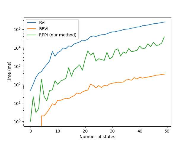
Figure 1: Runtime comparison on the Contamination Model with $n=1,\dots,50$ states.

Results on Frozen Lake

Table 1 shows our results on the Frozen Lake model. As mentioned before, due to RMDP structural restrictions imposed by the baselines, RVI is only applicable to the Unichain model whereas RRVI is applicable to neither of the models. Our RPPI imposes no structural restrictions on the RMDP and is thus applicable to both models.

As we can see from Table 1 our policy iteration-based RPPI is significantly faster than RVI, with an average runtime of 7.8 seconds. In contrast, the RVI method takes more than 2000 seconds on average, and times out on the $10\times 10$ model. Moreover, our method successfully solves all the Multichain model instances in less than 4 minutes each.

Table 1: Runtime comparison on the Frozen Lake model.

	Unichain		Multichain
$n$	RPPI Time (s)	VI Time (s)	RPPI Time (s)
2	0.0	0.15	0.0
3	0.0	8.3	2.6
4	0.0	156.8	0.6
5	0.1	106.6	4.0
6	6.1	1232.6	53.7
7	17.4	3347.8	119.0
8	3.7	7383.6	104.8
9	19.2	6496.6	93.0
10	23.7	Timeout	231.4
Average	7.8	2341.5	67.6
STDEV	9.5	3061.8	78.2

6 Conclusion

We considered the problem of solving long-run average reward robust Markov decision processes with polytopic uncertainty sets and proposed a new perspective on this problem by establishing a polynomial-time reduction to solving long-run average reward turn-based stochastic games. This reduction allowed us to leverage results from the stochastic games literature and obtain a number of results on computational complexity and efficient algorithms that were hitherto not known to hold for long-run average polytopic RMDPs. First, we show that the threshold decision problem for long-run average reward polytopic RMDPs is in $\textsc{NP}\cap\textsc{coNP}$ and that there exists a randomized algorithm with sub-exponential expected runtime for solving them. Second, we present Robust Polytopic Policy Iteration (RPPI), an algorithm for solving long-run average reward polytopic RMDPs based on policy iteration. Our experiments demonstrate significant computational runtime gains in comparison to state of the art value iteration-based algorithms applicable to polytopic RMDPs, and the ability to efficiently solve multichain polytopic RMDPs to which the existing algorithms are not applicable.

Our work leaves several interesting venues for future work. First, it would be very interesting to further explore the deep connection between polytopic RMDPs and stochastic games. Second, a natural question to consider is whether and how RMDPs with non-rectangular uncertainty sets could be related to stochastic games.

Acknowledgements

This work was supported in part by the ERC-2020- CoG 863818 (FoRM-SMArt).

Appendix

Appendix A Proof of Theorem 2

Theorem (Correctness).

Consider a polytopic RMDP $\mathcal{M}=(S^{\mathcal{M}},A^{\mathcal{M}},\mathcal{P}^{\mathcal{M}},r^{\mathcal{M}},s_{0}^{\mathcal{M}})$ and define a TBSG $\mathcal{G}^{\mathcal{M}}=(S^{\mathcal{G}_{\mathcal{M}}},A^{\mathcal{G}_{\mathcal{M}}},\delta^{\mathcal{G}_{\mathcal{M}}},r^{\mathcal{G}_{\mathcal{M}}},s_{0}^{\mathcal{G}_{\mathcal{M}}})$ as above. Then, for long-run average objective we have

$$\mathit{Val}^{*}(\mathcal{\mathcal{M}})=\mathit{Val}^{*}(\mathcal{G}^{\mathcal{M}}).$$

Proof.

Let $\Sigma^{\mathcal{M}}$ and $\Pi^{\mathcal{M}}$ denote the sets of all policies of the agent and the environment in the RMDP, and let $\Sigma^{\mathcal{G}_{\mathcal{M}}}$ and $\Pi^{\mathcal{G}_{\mathcal{M}}}$ denote the sets of all policies of the agent player and the environment player in the TBSG. We use $\Sigma^{\mathcal{M}}_{p}$, $\Pi^{\mathcal{M}}_{p}$, $\Sigma^{\mathcal{G}_{\mathcal{M}}}_{p}$ and $\Pi^{\mathcal{G}_{\mathcal{M}}}_{p}$ to denote the subsets of pure positional policies in these sets. Our proof proceeds in four steps. First, we define the mappings

$$\Phi:\Sigma^{\mathcal{M}}\rightarrow\Sigma^{\mathcal{G}_{\mathcal{M}}},\hskip 10.00002pt\Psi:\Pi^{\mathcal{M}}\rightarrow\Pi^{\mathcal{G}_{\mathcal{M}}}.$$

Second, we show that these mappings preserve the values of policy pairs. Third, we show that these mappings give rise to one-to-one correspondences (i.e. bijections) between pure positional policies in RMDPs and TBSGs

$$\Phi_{p}:\Sigma^{\mathcal{M}}_{p}\rightarrow\Sigma^{\mathcal{G}_{\mathcal{M}}}_{p},\hskip 10.00002pt\Psi_{p}:\Pi^{\mathcal{M}}_{p}\rightarrow\Pi^{\mathcal{G}_{\mathcal{M}}}_{p}.$$

Fourth, we use all the above ingredients to conclude the theorem claim and show that $\mathit{Val}^{*}(\mathcal{\mathcal{M}})=\mathit{Val}^{*}(\mathcal{G}^{\mathcal{M}})$.

Step 1: Definition of $\Phi$

Consider an RMDP agent policy

$$\sigma:(S^{\mathcal{M}}\times A^{\mathcal{M}})^{\ast}\times S^{\mathcal{M}}\rightarrow\Delta(A^{\mathcal{M}}).$$

We define a TBSG agent player policy

$$\Phi(\sigma):(S_{\max}^{\mathcal{G}_{\mathcal{M}}}\times A_{\max}^{\mathcal{G}_{\mathcal{M}}}\cup S_{\min}^{\mathcal{G}_{\mathcal{M}}}\times A_{\min}^{\mathcal{G}_{\mathcal{M}}})^{\ast}\times S_{\max}^{\mathcal{G}_{\mathcal{M}}}\rightarrow\Delta(A_{\max}^{\mathcal{G}_{\mathcal{M}}}).$$

as follows. In order to define $\Phi(\sigma)$, we need to specify $\Phi(\sigma)(h)$ for every Max-history $h$ in the TBSG $\mathcal{G}_{\mathcal{M}}$. Let $h$ be a Max-history in $\mathcal{G}_{\mathcal{M}}$. Since the adversary and the environment players alternate in turns in the TBSG $\mathcal{G}_{\mathcal{M}}$, the history $h$ must be of form $h=s_{0},a_{0},s_{1},a_{1},\dots,s_{2k-2},a_{2k-2},s_{2k-1},a_{2k-1},s_{2k}$ for some $k\in\mathbb{N}_{0}$, where even-indexed states and actions belong to the adversary player and odd-indexed states and actions belong to the environment player. Let $h^{\prime}=s_{0},a_{0},\dots,s_{2k-2},a_{2k-2},s_{2k}$ be the subsequence consisting only of states and actions belonging to the adversary player in $\mathcal{G}_{\mathcal{M}}$. Then $h^{\prime}$ defines a history in the RMDP, and we define

$$\Phi(\sigma)(h):=\sigma(h^{\prime})$$

where $\sigma(h^{\prime})$ is interpreted as a probability distribution over $A_{\max}^{\mathcal{G}_{\mathcal{M}}}$ which recall is defined as a copy of $A^{\mathcal{M}}$.

Step 1: Definition of $\Psi$

Consider an RMDP environment policy

$$\pi:(S^{\mathcal{M}}\times A^{\mathcal{M}})^{\ast}\times S^{\mathcal{M}}\times A^{\mathcal{M}}\rightarrow\mathcal{P}^{\mathcal{M}}.$$

We define a TBSG environment player policy

$$\Psi(\pi):(S_{\max}^{\mathcal{G}_{\mathcal{M}}}\times A_{\max}^{\mathcal{G}_{\mathcal{M}}}\cup S_{\min}^{\mathcal{G}_{\mathcal{M}}}\times A_{\min}^{\mathcal{G}_{\mathcal{M}}})^{\ast}\times S_{\min}^{\mathcal{G}_{\mathcal{M}}}\rightarrow\Delta(A_{\min}^{\mathcal{G}_{\mathcal{M}}}).$$

as follows. In order to define $\Psi(\pi)$, we need to specify $\Psi(\pi)(h)$ for every Min-history $h$ in the TBSG $\mathcal{G}_{\mathcal{M}}$. Let $h$ be a Min-history in $\mathcal{G}_{\mathcal{M}}$. Since the adversary and the environment players alternate in turns in the TBSG $\mathcal{G}_{\mathcal{M}}$, the history $h$ must be of form $h=s_{0},a_{0},s_{1},a_{1},\dots,s_{2k-2},a_{2k-2},s_{2k-1},a_{2k-1},s_{2k},a_{2k},s_{2k+1}$ for some $k\in\mathbb{N}_{0}$, where even-indexed states and actions belong to the adversary player and odd-indexed states and actions belong to the environment player. Let $h^{\prime}=s_{0},a_{0},\dots,s_{2k-2},a_{2k-2},s_{2k},a_{2k}$ be the subsequence consisting only of states and actions belonging to the adversary player in $\mathcal{G}_{\mathcal{M}}$. Then $h^{\prime}$ defines an environment history in the RMDP, and we define

$$\Psi(\pi)(h):=\pi(h^{\prime})$$

where $\pi(h^{\prime})$ is interpreted as a probability distribution over the vertices of the uncertainty polytope $\mathcal{P}^{\mathcal{M}}(s_{2k},a_{2k})$.

Step 2: Preservation of policy pair values

We now show that $\Phi$ and $\Psi$ preserve values of policy pairs, i.e. that

$$\mathit{Val}(\mathcal{M},\sigma,\pi)=\mathit{Val}(\mathcal{G}_{\mathcal{M}},\Phi(\sigma),\Psi(\pi))$$ (1)

holds for each $\sigma\in\Sigma^{\mathcal{M}}$ and $\pi\in\Pi^{\mathcal{M}}$ under long-run average objective. To prove this, we first recall the definitions of values in RMDPs and TBSGs. We have

$$\begin{split}&\mathit{Val}(\mathcal{M},\sigma,\pi)\\ &=\mathbb{E}^{\sigma,\pi}_{\mathcal{M}}\Big{[}\textsc{LimAvg}(S_{0}^{\mathcal{M}},A_{0}^{\mathcal{M}},S_{1}^{\mathcal{M}},A_{1}^{\mathcal{M}},\dots)\Big{]}\\ &=\mathbb{E}^{\sigma,\pi}_{\mathcal{M}}\Big{[}\liminf_{N\rightarrow\infty}\frac{1}{N+1}\cdot\sum_{i=0}^{N}r(S_{i}^{\mathcal{M}},A_{i}^{\mathcal{M}})\Big{]},\end{split}$$

where we use $S_{i}^{\mathcal{M}}$ and $A_{i}^{\mathcal{M}}$ to denote random variables defined as the $i$-th state and action in a random trajectory induced by the probability distribution over the space of all trajectories in the RMDP defined by policies $\sigma$ and $\pi$. Similarly, by our definition of the reward function in the TBSG $\mathcal{G}_{\mathcal{M}}$ which only incurs rewards in state-action pairs owned by the agent player, we have

$$\begin{split}&\mathit{Val}(\mathcal{G}_{\mathcal{M}},\Phi(\sigma),\Psi(\pi))\\ &=\mathbb{E}^{\Phi(\sigma),\Psi(\pi)}_{\mathcal{G}_{\mathcal{M}}}\Big{[}\textsc{LimAvg}(S_{0}^{\mathcal{G}_{\mathcal{M}}},A_{0}^{\mathcal{G}_{\mathcal{M}}},(S_{0}^{\mathcal{G}_{\mathcal{M}}},A_{0}^{\mathcal{G}_{\mathcal{M}}}),V_{0}^{\mathcal{G}_{\mathcal{M}}},\dots)\Big{]}\\ &=\mathbb{E}^{\Phi(\sigma),\Psi(\pi)}_{\mathcal{G}_{\mathcal{M}}}\Big{[}\liminf_{N\rightarrow\infty}\frac{1}{N+1}\cdot\sum_{i=0}^{N}r(S_{i}^{\mathcal{G}_{\mathcal{M}}},A_{i}^{\mathcal{G}_{\mathcal{M}}})\Big{]}\end{split}$$

where we use $S_{i}^{\mathcal{G}_{\mathcal{M}}}$, $A_{i}^{\mathcal{G}_{\mathcal{M}}}$, $V_{i}^{\mathcal{G}_{\mathcal{M}}}$ to denote random variables defined as the $i$-th state owned by the agent player, action owned by the agent player and uncertainty polytope vertex owned by the environment player in a random trajectory induced by the probability distribution over the space of all trajectories in the TBSG defined by policies $\Phi(\sigma)$ and $\Psi(\pi)$.

Hence, in order to prove eq. (1), by Dominated Convergence Theorem [Williams, 1991, Section 5.9] it suffices to show that for each $N\in\mathbb{N}$ we have

$$\begin{split}&\mathbb{E}^{\sigma,\pi}_{\mathcal{M}}\Big{[}\frac{\sum_{i=0}^{N}r(S_{i}^{\mathcal{M}},A_{i}^{\mathcal{M}})}{N+1}\Big{]}\\ &=\mathbb{E}^{\Phi(\sigma),\Psi(\pi)}_{\mathcal{G}_{\mathcal{M}}}\Big{[}\frac{\sum_{i=0}^{N}r(S_{i}^{\mathcal{G}_{\mathcal{M}}},A_{i}^{\mathcal{G}_{\mathcal{M}}})}{N+1}\Big{]}.\end{split}$$ (2)

Eq. (2) follows immediately by writing out the definition of the expected value and by proving that, for each $N\in\mathbb{N}$ and for each RMDP history $s_{0},a_{0},s_{1},a_{1},\dots,s_{N},a_{N}$, we have

$$\begin{split}&\mathbb{P}^{\sigma,\pi}_{\mathcal{M}}\Big{[}\bigwedge_{i=0}^{N}S_{i}^{\mathcal{M}}=s_{i}\land A_{i}^{\mathcal{M}}=A_{i}\Big{]}\\ &=\mathbb{P}^{\Phi(\sigma),\Psi(\pi)}_{\mathcal{G}_{\mathcal{M}}}\Big{[}\bigwedge_{i=0}^{N}S_{i}^{\mathcal{G}_{\mathcal{M}}}=s_{i}\land A_{i}^{\mathcal{G}_{\mathcal{M}}}=A_{i}\Big{]}.\end{split}$$

But this can be proved straightforwardly by induction on $N$, by our construction of the TBSG $\mathcal{G}_{\mathcal{M}}$ and by using Markov property in both RMDP and TBSG. Hence, eq. (1) follows.

Step 3: One-to-one correspondence between pure positional policies

Next, we observe that the mappings $\Phi$ and $\Psi$ become one-to-one correspondences when restricted to pure positional policies, i.e. that

$$\Phi_{p}:\Sigma^{\mathcal{M}}_{p}\rightarrow\Sigma^{\mathcal{G}_{\mathcal{M}}}_{p},\hskip 10.00002pt\Psi_{p}:\Pi^{\mathcal{M}}_{p}\rightarrow\Pi^{\mathcal{G}_{\mathcal{M}}}_{p}.$$

define bijections between pure positional policies in the RMDP $\mathcal{M}$ and the TBSG $\mathcal{G}_{\mathcal{M}}$. The facts that $\Phi_{p}$ and $\Psi_{p}$ are both injective and surjective follow immediately from our construction of maps $\Phi$ and $\Psi$ above.

Step 4: Conclusion of theorem proof

We conclude the theorem claim as follows. For every pair $\sigma$ and $\pi$ of an adversary and an environment policy in the RMDP $\mathcal{M}$, by Step 2 above we have that, under both long-run average and discounted-sum objectives,

$$\mathit{Val}(\mathcal{\mathcal{M}},\sigma,\pi)=\mathit{Val}(\mathcal{G}_{\mathcal{M}},\Phi(\sigma),\Psi(\pi)).$$

Hence, we have

$$\begin{split}\mathit{Val}^{*}(\mathcal{\mathcal{M}})&=\sup_{\sigma\in\Sigma^{\mathcal{M}}}\inf_{\pi\in\Pi^{\mathcal{M}}}\mathit{Val}(\mathcal{M},\sigma,\pi)\\ &=\sup_{\sigma\in\Sigma^{\mathcal{M}}}\inf_{\pi\in\Pi^{\mathcal{M}}}\mathit{Val}(\mathcal{G}_{\mathcal{M}},\Phi(\sigma),\Psi(\pi))\\ &\leq\sup_{\sigma\in\Sigma^{\mathcal{M}}}\inf_{\pi^{\prime}\in\Pi^{\mathcal{G}_{\mathcal{M}}}_{p}}\mathit{Val}(\mathcal{G}_{\mathcal{M}},\Phi(\sigma),\pi^{\prime})\\ &\leq\sup_{\sigma^{\prime}\in\Sigma^{\mathcal{G}_{\mathcal{M}}}}\inf_{\pi^{\prime}\in\Pi^{\mathcal{G}_{\mathcal{M}}}_{p}}\mathit{Val}(\mathcal{G}_{\mathcal{M}},\Phi(\sigma),\pi^{\prime})\\ &=\sup_{\sigma^{\prime}\in\Sigma^{\mathcal{G}_{\mathcal{M}}}_{p}}\inf_{\pi^{\prime}\in\Pi^{\mathcal{G}_{\mathcal{M}}}_{p}}\mathit{Val}(\mathcal{G}_{\mathcal{M}},\Phi(\sigma),\pi^{\prime})\\ &=\mathit{Val}^{*}(\mathcal{G}_{\mathcal{M}}),\end{split}$$

where in the second equality we used Step 2 above, in the third inequality we used the fact that pure positional policies are a subset of all policies and that $\Psi$ is a bijection when restricted to pure positional policies, in the fourth inequality we used that $\{\Phi(\sigma)\mid\sigma\in\Sigma^{\mathcal{M}}\}\subseteq\Sigma^{\mathcal{G}_{\mathcal{M}}}$ and in the last two equalities we used pure positional determinacy of TBSGs (Theorem 1 in the main paper).

On the other hand, by pure positional determinacy of TBSGs, we also know that there exist pure positional policies $\sigma^{\ast}\in\Sigma^{\mathcal{G}_{\mathcal{M}}}_{p}$ and $\pi^{\ast}\in\Pi^{\mathcal{G}_{\mathcal{M}}}_{p}$ such that $\mathit{Val}^{*}(\mathcal{G}_{\mathcal{M}})=\mathit{Val}(\mathcal{G}_{\mathcal{M}},\sigma^{\ast},\pi^{\ast})$. Then, by Steps 2 and 3 above, we also have $\mathit{Val}^{*}(\mathcal{G}_{\mathcal{M}})=\mathit{Val}(\mathcal{M},\Phi^{-1}(\sigma^{\ast}),\Psi^{-1}(\pi^{\ast}))$. Hence, as above we showed that $\mathit{Val}^{*}(\mathcal{\mathcal{M}})\leq\mathit{Val}^{*}(\mathcal{G}^{\mathcal{M}})$ we conclude that $\Phi^{-1}(\sigma^{\ast})$ and $\Psi^{-1}(\pi^{\ast})$ achieve optimal payoffs in the RMDP $\mathcal{M}$ and thus conclude that $\mathit{Val}^{*}(\mathcal{\mathcal{M}})=\mathit{Val}^{*}(\mathcal{G}^{\mathcal{M}})$. ∎

Appendix B Proof of Theorem 3

Theorem (Complexity).

Consider a polytopic RMDP $\mathcal{M}=(S^{\mathcal{M}},A^{\mathcal{M}},\mathcal{P}^{\mathcal{M}},r^{\mathcal{M}},s_{0}^{\mathcal{M}})$ and define a TBSG $\mathcal{G}^{\mathcal{M}}=(S^{\mathcal{G}_{\mathcal{M}}},A^{\mathcal{G}_{\mathcal{M}}},\delta^{\mathcal{G}_{\mathcal{M}}},r^{\mathcal{G}_{\mathcal{M}}},s_{0}^{\mathcal{G}_{\mathcal{M}}})$ as in Section 3 of the paper. Then, the size of $\mathcal{G}^{\mathcal{M}}$ is polynomial in the size of $\mathcal{M}$.

Proof.

We need to show that each element of the tuple $\mathcal{G}^{\mathcal{M}}=(S^{\mathcal{G}_{\mathcal{M}}},A^{\mathcal{G}_{\mathcal{M}}},\delta^{\mathcal{G}_{\mathcal{M}}},r^{\mathcal{G}_{\mathcal{M}}},s_{0}^{\mathcal{G}_{\mathcal{M}}})$ is of size polynomial in the size of the elements of the tuple $\mathcal{M}=(S^{\mathcal{M}},A^{\mathcal{M}},\mathcal{P}^{\mathcal{M}},r^{\mathcal{M}},s_{0}^{\mathcal{M}})$.

Before we prove this claim, recall that we assume that each polytopic RMDP is represented as an ordered tuple $\mathcal{M}=(S^{\mathcal{M}},A^{\mathcal{M}},\mathcal{P}^{\mathcal{M}},r^{\mathcal{M}},s_{0}^{\mathcal{M}})$, where $S^{\mathcal{M}}$ is a list of states, $A^{\mathcal{M}}$ is a list of actions, $\mathcal{P}^{\mathcal{M}}$ is a list of polytope vertices for each state-action pair, $r^{\mathcal{M}}$ is a list of rewards for each state-action pair and $s_{0}^{\mathcal{M}}$ is an element of the state list.

We now show prove the desired claim:

• States. We have $S^{\mathcal{G}_{\mathcal{M}}}=S^{\mathcal{G}_{\mathcal{M}}}_{\max}\cup S^{\mathcal{G}_{\mathcal{M}}}_{\min}$, where $S^{\mathcal{G}_{\mathcal{M}}}_{\max}=S^{\mathcal{M}}$ and $S^{\mathcal{G}_{\mathcal{M}}}_{\min}=S^{\mathcal{M}}\times A^{\mathcal{M}}$. Hence,

  $$|S^{\mathcal{G}_{\mathcal{M}}}|\in\mathcal{O}(|S^{\mathcal{M}}|+|S^{\mathcal{M}}|\cdot|A^{\mathcal{M}}|),$$

  which is polynomial in the size of the RMDP.

• Actions. We have $A^{\mathcal{G}_{\mathcal{M}}}=A^{\mathcal{G}_{\mathcal{M}}}_{\max}\cup A^{\mathcal{G}_{\mathcal{M}}}_{\min}$, where $A^{\mathcal{G}_{\mathcal{M}}}_{\max}=A^{\mathcal{M}}$ and $A^{\mathcal{G}_{\mathcal{M}}}_{\min}=\cup_{(s,a)\in S^{\mathcal{M}}\times A^{\mathcal{M}}}V^{\mathcal{M}}_{s,a}$. Hence,

  $$\begin{split}|A^{\mathcal{G}_{\mathcal{M}}}|&\in\mathcal{O}\Big{(}|A^{\mathcal{M}}|+\sum_{(s,a)\in S^{\mathcal{M}}\times A^{\mathcal{M}}}|V^{\mathcal{M}}_{s,a}|\Big{)}\\ &=\mathcal{O}(|A^{\mathcal{M}}|+|\mathcal{P}^{\mathcal{M}}|),\end{split}$$

  which is polynomial in the size of the RMDP.

• Transition function. Since $\delta^{\mathcal{G}_{\mathcal{M}}}:S{{}^{\mathcal{G}}_{\mathcal{M}}}_{\max}\times A{{}^{\mathcal{G}}_{\mathcal{M}}}_{\max}\cup S{{}^{\mathcal{G}}_{\mathcal{M}}}_{\min}\times A{{}^{\mathcal{G}}_{\mathcal{M}}}_{\min}\rightarrow\Delta(S{{}^{\mathcal{G}}_{\mathcal{M}}})$, we have

  $$\begin{split}|\delta^{\mathcal{G}_{\mathcal{M}}}|&=\sum_{(s,a)\in S{{}^{\mathcal{G}}_{\mathcal{M}}}_{\max}\times A{{}^{\mathcal{G}}_{\mathcal{M}}}_{\max}}|\delta^{\mathcal{G}_{\mathcal{M}}}(s,a)|\\ &+\sum_{((s,a),v)\in S{{}^{\mathcal{G}}_{\mathcal{M}}}_{\min}\times A{{}^{\mathcal{G}}_{\mathcal{M}}}_{\min}}|\delta^{\mathcal{G}_{\mathcal{M}}}((s,a),v)|.\end{split}$$

  For each $(s,a)\in S{{}^{\mathcal{G}}_{\mathcal{M}}}_{\max}\times A{{}^{\mathcal{G}}_{\mathcal{M}}}_{\max}$, we have that $\delta^{\mathcal{G}_{\mathcal{M}}}(s,a)$ is a Dirac probability distribution so is of constant size. On the other hand, for each $((s,a),v)\in S{{}^{\mathcal{G}}_{\mathcal{M}}}_{\min}\times A{{}^{\mathcal{G}}_{\mathcal{M}}}_{\min}$, we have that $\delta^{\mathcal{G}_{\mathcal{M}}}((s,a),v)$ is of the same size as the probability distribution stored in the vertex $v$ of the uncertainty polytope $V^{\mathcal{M}}_{s,a}$. Hence, we conclude that

  $$|\delta^{\mathcal{G}_{\mathcal{M}}}|\in\mathcal{O}(|S^{\mathcal{M}}|\cdot|A^{\mathcal{M}}|+|S^{\mathcal{M}}|\cdot|A^{\mathcal{M}}|\cdot|\mathcal{P}|),$$

  which is polynomial in the size of the RMDP.

• Reward function. Since $r^{\mathcal{G}_{\mathcal{M}}}:S{{}^{\mathcal{G}}_{\mathcal{M}}}_{\max}\times A{{}^{\mathcal{G}}_{\mathcal{M}}}_{\max}\cup S{{}^{\mathcal{G}}_{\mathcal{M}}}_{\min}\times A{{}^{\mathcal{G}}_{\mathcal{M}}}_{\min}\rightarrow\mathbb{R}$ is defined to coincide with $2\cdot r^{\mathcal{M}}$ on state-action pairs belonging to Max and is set to be $0$ on state-action pairs belonging to Min, we conclude that

  $$|r^{\mathcal{G}_{\mathcal{M}}}|\in\mathcal{O}(|r^{\mathcal{M}}|+|S^{\mathcal{M}}|\cdot|A^{\mathcal{M}}|),$$

  which is polynomial in the size of the RMDP.

• Initial state. Since $s_{0}^{\mathcal{G}_{\mathcal{M}}}=s_{0}^{\mathcal{M}}\in S^{\mathcal{G}_{\mathcal{M}}}_{\max}$, i.e. the initial state in $\mathcal{G}^{\mathcal{M}}$ is the copy of the initial state in $\mathcal{M}$, we have

  $$|s_{0}^{\mathcal{G}_{\mathcal{M}}}|\in\mathcal{O}(|s_{0}^{\mathcal{M}}|),$$

  which is polynomial in the size of the RMDP.

Hence, the size of the TBSF $\mathcal{G}_{\mathcal{M}}$ is polynomial in the size of the RMDP $\mathcal{M}$, as claimed. ∎

Appendix C Extending Theorem 2 to Discounted Payoff

A slight modification of the reduction described in Section 3 allows reducing discounted-sum reward polytopic RMDPs to discounted-sum reward TBSGs: we just omit the doubling of reward functions and define

$$r^{\mathcal{G}_{\mathcal{M}}}(s,a)=r^{\mathcal{M}}(s,a).$$

for each state-action pair $s,a$. However, the fact that two turns in $\mathcal{G}_{\mathcal{M}}$ (one turn per player) correspond to a single step in $\mathcal{M}$ poises another issue: in $\mathcal{G}_{\mathcal{M}}$, the discounting proceeds twice as fast compared to $\mathcal{M}$. A mathematically simple solution to this issue is to define the discount factor in $\mathcal{G}_{\mathcal{M}}$ to be the square root of the original discount factor $\gamma$ from $\mathcal{G}_{\mathcal{M}}$. However, this is problematic from an algorithmic point of view, since $\sqrt{\gamma}$ might be irrational. Hence, we propose a different modification of the reduction: first reduce discounted RMDPs to terminal-reward RMDPs and then reduce the latter to terminal-reward TBSGs using a similar reduction as in Section 3.

Terminal-Reward Objectives

The first step of our reduction mimics the well-known reduction from discounted TBSGs to terminal-reward TBSGs presented, e.g., in Andersson and Miltersen [2009]. Terminal-reward TBSGs are TBSGs with a distinguished set of terminal states $T$ and an additional sink state $\bot$ (i.e., $\delta(\bot,a)(\bot)=1$ for each action $a$). Similarly, from each terminal state $t\in T$ and each action $a$, we have $\delta(t,a)(\bot)=1$. Finally, the reward function $r$ satisfies $r(s,a)=0$ for each $s\not\in T$. That is, the rewards can only be accrued in terminal states, and hence only once per trajectory. The objective considered is the expected undiscounted total reward, i.e. the expected value of the reward encountered when transitioning from a terminal state to $\bot$.

The idea behind the reduction is the well-known observation that discounted MDPs/games are equivalent to non-discounted ones in which in every step there is a probability $\gamma$ of terminating the interaction with the MDP/game.

Formally, to each discounted-sum reward polytopic RMDP $\mathcal{M}$ with discount factor $\gamma$ we can assign a terminal-reward RMDP $\mathcal{M}_{TR}$ as follows:

• The states of $\mathcal{M}_{TR}$ are $S\cup T\cup\{\bot\}$, where $S$ is the set of states in $\mathcal{M}$ and

  $$T=\{t_{(s,a)}\mid(s,a)\in S\times A\},$$

  where $A$ is the set of actions in $\mathcal{M}$.

• The action sets of $\mathcal{M}$ and $\mathcal{M}_{TR}$ are identical.

• The transition function $\delta_{TR}$ of $\mathcal{M}_{TR}$ is defined as follows: for each $s,s^{\prime}\in S$ and $a\in A$ we have $\delta_{TR}(s,a)(t_{s,a})=1-\gamma$ and $\delta_{TR}(s,a)(s^{\prime})=\delta(s,a)(s)\cdot\gamma$. Apart from that, we have the transitions from terminal states and $\bot$ as defined above.

• The reward function $r_{TR}$ of $\mathcal{M}_{TR}$ is defined as follows: For each $t_{(s,a)}\in T$ and $a\in A$ we have $r_{TR}(t_{(s,a)},a)=r(s,a)/(1-\gamma)$. All other rewards are $0$.

• The initial states of both RMDPs are identical.

The reduction clearly runs in polynomial time. Also, there is a straightforward one-to-one correspondence between policies in $\mathcal{M}$ and $\mathcal{M}_{TR}$, hence we consider the policy sets of the two models to be equal. We can prove that the correspondence preserves the expected payoffs of the policies, yielding a reduction from discounted-payoff RMDPs to terminal reward RMDPs.

Theorem 5.

For any policy $\pi$ it holds

$$\mathbb{E}^{\pi}_{\mathcal{M}}[\textsc{Disc}_{\gamma}]=\mathbb{E}^{\pi}_{\mathcal{M}_{TR}}[\textsc{Term}],$$

where Term is the reward accrued when transitioning from a terminal state to $\bot$.

Proof.

We use the same notation as in the proof of Theorem 2. We have

$$\begin{split}&\mathbb{E}^{\pi}_{\mathcal{M}_{TR}}[\textsc{Term}]=\\ &=\sum_{i=0}^{\infty}\sum_{(s,a)\in S\times A}\mathbb{P}^{\pi}_{\mathcal{M}_{TR}}[S_{i+1}=t_{(s,a)}]\cdot r_{TR}(t_{(s,a)})\\ &=\sum_{i=0}^{\infty}\sum_{(s,a)\in S\times A}\mathbb{P}^{\pi}_{\mathcal{M}_{TR}}[S_{i+1}=t_{(s,a)}]\cdot\frac{r(s,a)}{1-\gamma}\\ &=\sum_{i=0}^{\infty}\sum_{(s,a)\in S\times A}(1-\gamma)\cdot\gamma^{i}\cdot\mathbb{P}^{\pi}_{\mathcal{M}}[S_{i}=s\wedge A_{i}=a]\cdot\frac{r(s,a)}{1-\gamma}\\ &=\sum_{i=0}^{\infty}\sum_{(s,a)\in S\times A}\mathbb{P}^{\pi}_{\mathcal{M}}[S_{i}=s\wedge A_{i}=a]\cdot\gamma^{i}\cdot{r(s,a)}\\ &=\mathbb{E}^{\pi}_{\mathcal{M}}[\textsc{Disc}_{\gamma}].\end{split}$$

∎

From Terminal Reward RMDPs to TBSGs

We can use the reduction from Section 3 (without doubling of the rewards), to convert (in polynomial time) a polytopic terminal reward RMDP into a terminal reward TBSG with the same optimal values. (Note that when applying the reduction from Section 3, there are no transitions to terminal states on turns of player Min.) Terminal reward TBSGs then reduce in polynomial time to simple stochastic games (SSGs) Andersson and Miltersen [2009], which are known to be purely positionally determined, solvable in $\textsc{NP}\cap\textsc{coNP}$, and which admit randomized sub-exponential solution algorithms. Hence, Corollaries 1–3 hold also for RMDPs with discounted payoff objectives.

References

- Andersson and Miltersen [2009] Daniel Andersson and Peter Bro Miltersen. The complexity of solving stochastic games on graphs. In Yingfei Dong, Ding-Zhu Du, and Oscar Ibarra, editors, Algorithms and Computation, pages 112–121, Berlin, Heidelberg, 2009. Springer Berlin Heidelberg.
- Bertrand et al. [2023] Nathalie Bertrand, Patricia Bouyer-Decitre, Nathanaël Fijalkow, and Mateusz Skomra. Stochastic games. In Nathanaël Fijalkow, editor, Games on Graphs. 2023.
- Condon [1992] A. Condon. The Complexity of Stochastic Games. Information and Computation, 96(2):203–224, 1992.
- Filar and Vrieze [1996] J. Filar and K. Vrieze. Competitive Markov Decision Processes. 1996.
- Ghavamzadeh et al. [2016] Mohammad Ghavamzadeh, Marek Petrik, and Yinlam Chow. Safe policy improvement by minimizing robust baseline regret. In Daniel D. Lee, Masashi Sugiyama, Ulrike von Luxburg, Isabelle Guyon, and Roman Garnett, editors, Advances in Neural Information Processing Systems 29: Annual Conference on Neural Information Processing Systems 2016, December 5-10, 2016, Barcelona, Spain, pages 2298–2306, 2016.
- Gillette [1957] G. Gillette. Stochastic Games with Zero Stop Probabilities. Contributions to the Theory of Games, vol III, pages 179–187, 1957.
- Givan et al. [2000] Robert Givan, Sonia M. Leach, and Thomas L. Dean. Bounded-parameter markov decision processes. Artif. Intell., 122(1-2):71–109, 2000.
- Goyal and Grand-Clément [2023] Vineet Goyal and Julien Grand-Clément. Robust markov decision processes: Beyond rectangularity. Math. Oper. Res., 48(1):203–226, 2023.
- Grand-Clément and Petrik [2023] Julien Grand-Clément and Marek Petrik. Reducing blackwell and average optimality to discounted mdps via the blackwell discount factor. CoRR, abs/2302.00036, 2023.
- Grand-Clement et al. [2023] Julien Grand-Clement, Marek Petrik, and Nicolas Vieille. Beyond discounted returns: Robust markov decision processes with average and blackwell optimality. arXiv preprint arXiv:2312.03618, 2023.
- Hansen et al. [2013] Thomas Dueholm Hansen, Peter Bro Miltersen, and Uri Zwick. Strategy iteration is strongly polynomial for 2-player turn-based stochastic games with a constant discount factor. J. ACM, 60(1):1:1–1:16, 2013.
- Hensel et al. [2022] Christian Hensel, Sebastian Junges, Joost-Pieter Katoen, Tim Quatmann, and Matthias Volk. The probabilistic model checker storm. Int. J. Softw. Tools Technol. Transf., 24(4):589–610, 2022.
- Ho et al. [2018] Chin Pang Ho, Marek Petrik, and Wolfram Wiesemann. Fast bellman updates for robust mdps. In Jennifer G. Dy and Andreas Krause, editors, Proceedings of the 35th International Conference on Machine Learning, ICML 2018, Stockholmsmässan, Stockholm, Sweden, July 10-15, 2018, volume 80 of Proceedings of Machine Learning Research, pages 1984–1993. PMLR, 2018.
- Ho et al. [2021] Chin Pang Ho, Marek Petrik, and Wolfram Wiesemann. Partial policy iteration for l1-robust markov decision processes. J. Mach. Learn. Res., 22:275:1–275:46, 2021.
- Iyengar [2005] Garud N. Iyengar. Robust dynamic programming. Math. Oper. Res., 30(2):257–280, 2005.
- Kaufman and Schaefer [2013] David L. Kaufman and Andrew J. Schaefer. Robust modified policy iteration. INFORMS J. Comput., 25(3):396–410, 2013.
- Kučera [2011] A. Kučera. Turn-Based Stochastic Games. In K.R. Apt, E. Grädel (Eds.): Lectures in Game Theory for Computer Scientists, pages 146–184. Cambridge University Press, 2011.
- Liggett and Lippman [1969] T.M. Liggett and S.A. Lippman. Stochastic Games with Perfect Information and Time Average Payoff. SIAM Review, 11(4):604–607, 1969.
- Ludwig [1995] W. Ludwig. A Subexponential Randomized Algorithm for the Simple Stochastic Game Problem. 117(1):151–155, 1995.
- Nilim and Ghaoui [2003] Arnab Nilim and Laurent El Ghaoui. Robustness in markov decision problems with uncertain transition matrices. In Sebastian Thrun, Lawrence K. Saul, and Bernhard Schölkopf, editors, Advances in Neural Information Processing Systems 16 [Neural Information Processing Systems, NIPS 2003, December 8-13, 2003, Vancouver and Whistler, British Columbia, Canada], pages 839–846. MIT Press, 2003.
- Puterman [1994] Martin L. Puterman. Markov Decision Processes: Discrete Stochastic Dynamic Programming. Wiley Series in Probability and Statistics. Wiley, 1994.
- Roy et al. [2017] Aurko Roy, Huan Xu, and Sebastian Pokutta. Reinforcement learning under model mismatch. In Isabelle Guyon, Ulrike von Luxburg, Samy Bengio, Hanna M. Wallach, Rob Fergus, S. V. N. Vishwanathan, and Roman Garnett, editors, Advances in Neural Information Processing Systems 30: Annual Conference on Neural Information Processing Systems 2017, December 4-9, 2017, Long Beach, CA, USA, pages 3043–3052, 2017.
- Shapley [1953] L.S. Shapley. Stochastic Games. Proceedings of the National Academy of Sciences, 39:1095–1100, 1953.
- Sutton et al. [1999] Richard S. Sutton, David A. McAllester, Satinder Singh, and Yishay Mansour. Policy gradient methods for reinforcement learning with function approximation. In Sara A. Solla, Todd K. Leen, and Klaus-Robert Müller, editors, Advances in Neural Information Processing Systems 12, [NIPS Conference, Denver, Colorado, USA, November 29 - December 4, 1999], pages 1057–1063. The MIT Press, 1999.
- Tamar et al. [2014] Aviv Tamar, Shie Mannor, and Huan Xu. Scaling up robust mdps using function approximation. In Proceedings of the 31th International Conference on Machine Learning, ICML 2014, Beijing, China, 21-26 June 2014, volume 32 of JMLR Workshop and Conference Proceedings, pages 181–189. JMLR.org, 2014.
- Tessler et al. [2019] Chen Tessler, Yonathan Efroni, and Shie Mannor. Action robust reinforcement learning and applications in continuous control. In Kamalika Chaudhuri and Ruslan Salakhutdinov, editors, Proceedings of the 36th International Conference on Machine Learning, ICML 2019, 9-15 June 2019, Long Beach, California, USA, volume 97 of Proceedings of Machine Learning Research, pages 6215–6224. PMLR, 2019.
- Tewari and Bartlett [2007] Ambuj Tewari and Peter L. Bartlett. Bounded parameter markov decision processes with average reward criterion. In Nader H. Bshouty and Claudio Gentile, editors, Learning Theory, 20th Annual Conference on Learning Theory, COLT 2007, San Diego, CA, USA, June 13-15, 2007, Proceedings, volume 4539 of Lecture Notes in Computer Science, pages 263–277. Springer, 2007.
- Towers et al. [2023] Mark Towers, Jordan K. Terry, Ariel Kwiatkowski, John U. Balis, Gianluca de Cola, Tristan Deleu, Manuel Goulão, Andreas Kallinteris, Arjun KG, Markus Krimmel, Rodrigo Perez-Vicente, Andrea Pierré, Sander Schulhoff, Jun Jet Tai, Andrew Tan Jin Shen, and Omar G. Younis. Gymnasium, March 2023.
- Wang and Zou [2021] Yue Wang and Shaofeng Zou. Online robust reinforcement learning with model uncertainty. In Marc’Aurelio Ranzato, Alina Beygelzimer, Yann N. Dauphin, Percy Liang, and Jennifer Wortman Vaughan, editors, Advances in Neural Information Processing Systems 34: Annual Conference on Neural Information Processing Systems 2021, NeurIPS 2021, December 6-14, 2021, virtual, pages 7193–7206, 2021.
- Wang and Zou [2022] Yue Wang and Shaofeng Zou. Policy gradient method for robust reinforcement learning. In Kamalika Chaudhuri, Stefanie Jegelka, Le Song, Csaba Szepesvári, Gang Niu, and Sivan Sabato, editors, International Conference on Machine Learning, ICML 2022, 17-23 July 2022, Baltimore, Maryland, USA, volume 162 of Proceedings of Machine Learning Research, pages 23484–23526. PMLR, 2022.
- Wang et al. [2023] Yue Wang, Alvaro Velasquez, George K. Atia, Ashley Prater-Bennette, and Shaofeng Zou. Robust average-reward markov decision processes. In Brian Williams, Yiling Chen, and Jennifer Neville, editors, Thirty-Seventh AAAI Conference on Artificial Intelligence, AAAI 2023, Thirty-Fifth Conference on Innovative Applications of Artificial Intelligence, IAAI 2023, Thirteenth Symposium on Educational Advances in Artificial Intelligence, EAAI 2023, Washington, DC, USA, February 7-14, 2023, pages 15215–15223. AAAI Press, 2023.
- Wiesemann et al. [2013] Wolfram Wiesemann, Daniel Kuhn, and Berç Rustem. Robust markov decision processes. Math. Oper. Res., 38(1):153–183, 2013.
- Williams [1991] David Williams. Probability with Martingales. Cambridge mathematical textbooks. Cambridge University Press, 1991.
- Yang et al. [2022] Wenhao Yang, Liangyu Zhang, and Zhihua Zhang. Toward theoretical understandings of robust markov decision processes: Sample complexity and asymptotics. The Annals of Statistics, 50(6):3223–3248, 2022.