Multi-Agent Probabilistic Ensembles with Trajectory Sampling for Connected Autonomous Vehicles
Abstract
Autonomous Vehicles (AVs) have attracted significant attention in recent years and Reinforcement Learning (RL) has shown remarkable performance in improving the autonomy of vehicles. In that regard, the widely adopted Model-Free RL (MFRL) promises to solve decision-making tasks in connected AVs (CAVs), contingent on the readiness of a significant amount of data samples for training. Nevertheless, it might be infeasible in practice and possibly lead to learning instability. In contrast, Model-Based RL (MBRL) manifests itself in sample-efficient learning, but the asymptotic performance of MBRL might lag behind the state-of-the-art MFRL algorithms. Furthermore, most studies for CAVs are limited to the decision-making of a single AV only, thus underscoring the performance due to the absence of communications. In this study, we try to address the decision-making problem of multiple CAVs with limited communications and propose a decentralized Multi-Agent Probabilistic Ensembles with Trajectory Sampling algorithm MA-PETS. In particular, in order to better capture the uncertainty of the unknown environment, MA-PETS leverages Probabilistic Ensemble (PE) neural networks to learn from communicated samples among neighboring CAVs. Afterwards, MA-PETS capably develops Trajectory Sampling (TS)-based model-predictive control for decision-making. On this basis, we derive the multi-agent group regret bound affected by the number of agents within the communication range and mathematically validate that incorporating effective information exchange among agents into the multi-agent learning scheme contributes to reducing the group regret bound in the worst case. Finally, we empirically demonstrate the superiority of MA-PETS in terms of the sample efficiency comparable to MFBL.
Index Terms:
Autonomous vehicle control, multi-agent model-based reinforcement learning, probabilistic ensembles with trajectory sampling.I Introduction
Recently, there emerges significant research interest towards Connected Autonomous Vehicles (CAVs) with a particular emphasis on developing suitable Reinforcement Learning (RL)-driven controlling algorithms [2, 3] for the optimization of intelligent traffic flows [4], decision making [5], and control of AVs [6]. Notably, the research on Multi-Agent Reinforcement Learning (MARL) makes significant progress in capably learning complex tasks for CAVs, through effective interaction between agents and the environment. Existing MARL methods for CAVs can be classified as Model-Free Reinforcement Learning (MFRL) and Model-Based Reinforcement Learning (MBRL), the key differences of which lie in whether agents estimate an explicit environment model for the policy learning [7].
Conventionally, MFRL, which relies on collected rewards on recorded state-action transition pairs, has been widely applied to model complex mixed urban traffic systems in multi-vehicle scenarios, showing excellent performance in various situations of autonomous driving [8, 9]. Typical examples of MFRL include MADDPG [10], COMA [11], QMIX [12], SVMIX[13]. However, the computational complexity of most MFRL algorithms grows exponentially with the number of agents. In order to solve training data scarcity-induced out-of-distribution (OOD) problems, MFRL is typically required to repetitively interact with the real-world to collect a sufficient amount of training data, which might be infeasible in practice and possibly lead to learning instability and huge overhead. On the contrary, due to the impressive sample efficiency, MBRL promises to solve CAVs issues[14] more capably and starts to attain some research interest [15, 16].
Typically, MBRL is contingent on learning an accurate probabilistic dynamics model that can clearly distinguish between aleatoric and epistemic uncertainty [17], where the former is inherent to the system noise, while the latter stems from sample scarcity and contributes to solving the OOD problem to a certain extent. Afterwards, based on the learned dynamics model from the collected data, MBRL undergoes a planning and control phase by simulating model-consistent transitions and optimizing the policy accordingly. However, the asymptotic performance of MBRL algorithms has lagged behind state-of-the-art MFRL methods in common benchmark tasks, especially as the environmental complexity increases. In other words, although MBRL algorithms tend to learn faster, they often converge to poorer results [18, 19]. Fortunately, extending single-agent RL [20] to a multi-agent case through efficient communication can compensate for the learning deficiency to some extent. In that regard, despite the simplicity of assuming the existence of a central controller, it might be practically infeasible or cost-effective to install such a controller in many real-world scenarios. Meanwhile, it is often challenging to establish fully connected communication between all agents, where the required communication overhead can scale exponentially[8, 10]. Instead, a more complex communication-limited decentralized multi-agent MBRL for CAVs becomes feasible, and specifying a suitable protocol for cooperation between agents turns crucial.
On the other hand, in order to theoretically characterise the sampling efficiency of RL, the concept of the regret bound emerges, which targets to theoretically measure the -time-step difference between an agent’s accumulated rewards and the total reward that an optimal policy (for that agent) would have achieved. Without loss of generality, for an -episodic RL environment with states and actions, contingent on Hoeffding inequality and Bernstein inequality, tabular upper-confidence bound (UCB) algorithms can lead to a regret bound of and respectively [21, 22], where hides the logarithmic factors. On the other hand, for any communicating Markov decision process (MDP) with the diameter , Jaksch et al. propose a classical confidence upper bound algorithm UCRL2 algorithm (abbreviation of Upper Confidence bound for RL) to achieve the regret bound . In the literature, there only sheds a little light on the regret bound of collaborative MARL. In this paper, inspired by the regret bound of UCRL2, we investigate the regret bound of decentralized communication-limited MBRL, and demonstrate how communication among the multi-agents can be used to reduce the regret bound and boost the learning performance.
In this paper, targeted at addressing the sample efficiency issue in a communication-limited multi-agent scenario, we propose a fully decentralized Multi-Agent Probabilistic Ensembles with Trajectory Sampling (MA-PETS) algorithm. In particular, MA-PETS could effectively exchange collected samples from individual agents to neighboring vehicles within a certain range, and extend the widely adopted single-agent Probabilistic Ensemble (PE) technique to competently reduce both aleatoric and epistemic uncertainty while fitting the multi-agent environmental transition. Furthermore, MA-PETS leverages computation-efficient Model Predictive Control (MPC)[23], which avoids gradient computations and exhibits appealing robustness to uncertainty, to produce suitable control actions from learned-model-based Trajectory Sampling (TS). Compared to the existing literature, the contribution of the paper can be summarized as follows:
-
•
We formulate the decentralized multi-agent decision-making issue for CAVs as parallel time-homogeneous Markov Decision Process (MDP), and devise a sample efficient MBRL solution MA-PETS.
-
•
Within MA-PETS, we develop a multi-agent PE to learn the unknown environmental transition dynamics model from exchanged data samples and calibrate TS-based MPC for model-based decision-making.
-
•
We analyze the group regret bound of MA-PETS on top of UCRL2, which theoretically demonstrates that multiple agents jointly exploring the state-action space in similar environments could communicate to discover the optimal policy faster than individual agents operating in parallel. On top of the concept of clique cover [24] of a communication undirected graph, our work mathematically verifies that in the worst case, the addition of more information from communication to a multi-agent algorithm still yields a sub-linear group regret concerning the number of agents and accelerates convergence. Thus, our theoretical derivation is completely different from [25], which takes the simple superposition of single-agent regret bounds.
-
•
We further illustrate our approach experimentally on a CAV simulation platform SMARTS [26] and validate the superiority of our proposed algorithm over other MARL methods in terms of sample efficiency. Besides, we evaluate the impact of communication ranges on MA-PETS and demonstrate the contributing effects of information exchange.
| Notation | Parameters Description |
|---|---|
| Number of RL agents | |
| Communication range | |
| Speed per vehicle at time-step | |
| Position per vehicle at | |
| Target velocity per vehicle at | |
| Speed of vehicles ahead and behind | |
| Distance of vehicles ahead and behind | |
| Travel distance per vehicle at | |
| No. of episodes | |
| Length per episode | |
| No. of Ensembles for dynamics Model | |
| Horizon of MPC | |
| Candidate action sequences in CEM | |
| Elite candidate action sequences in CEM | |
| No. of particles | |
| Max iteration of CEM | |
| Number of state-action visits in the episode | |
| Number of state-action visits before episode | |
| Cliques cover of | |
| Minimum number of cliques cover |
The remainder of the paper is organized as follows. Section II briefly introduces the related works. In Section III, we introduce the preliminaries of MDPs and formulate the system model. In Section IV and Section V, we present the details of MA-PETS and unveil the effect of communication range on the convergence of the MARL via the group regret bound, respectively. Finally, Section VI demonstrates the effectiveness and superiority MA-PETS through extensive simulations. We conclude the paper in Section VII.
II Related Works
II-A Multi-Agent Reinforcement Learning of CAVs
Decision-making of CAVs in high-density mixed-traffic intersections is a challenging task. A set of different MARL approaches have been proposed to solve the decision-making of AVs at unsignalised intersections [27], so as to improve traffic efficiency and safety, and show remarkable performance in various CAV cases. For instance, within the actor-critic MFRL framework, [11] introduces the multi-agent actor-critic method COMA that employs a centralized critic for estimating the -function, alongside decentralized actors to optimize policies. In a similar vein, [10] proposes using a central critic for centralized training coupled with multiple actors for distributed execution. However, a notable challenge arises as the number of agents increases or the action space expands, the computational complexity of MFRL algorithms like COMA escalates exponentially. To mitigate this computational burden, [12] proposes QMIX to involve the value decomposition of the joint value function into separate individual value functions for each agent. In addition, some researchers focus on the communication between agents. [13] proposes to adopt a stochastic graph neural network to capture the dynamic topological features of time-varying graphs while decomposing the value function. Nevertheless, the MFRL algorithm still suffers from high overhead due to the significant number of required calculations and samples.
II-B Model-Based Reinforcement Learning
To address the sampling efficiency and communication overhead issues in MFRL, MBRL naturally emerges as an alternative solution. Unfortunately, MBRL suffers from performance deficiency, as it might fail to accurately estimate the uncertainty in the environment and characterize the dynamics model, which belongs to a critical research component in MBRL. For example, [28] proposes a DNN-based method that is, to some extent, qualified to separate aleatoric and epistemic uncertainty while maintaining appropriate generalization capabilities, while PILCO [29] marginalizes aleatoric and epistemic uncertainty of a learned dynamics model to optimize the expected performance. Another type of MBRL falls within the scope of Dyna-style methods [30], where additional data to improve the efficiency of the RL is generated from interactions between the RL and the virtual environment. [31] proposes an RL training algorithm MA-PPO that incorporates a prior model into PPO algorithm to speed up the learning process while maintaining the sampling efficiency. [19] takes advantage of Model Predictive Control (MPC) to optimize the RL agent’s behavior policy by predicting and planning within the modeled virtual environment at each training step. Until recently, [15] proposes an uncertainty-aware MBRL and verifies that it has competitive performance as the state-of-the-art MFRL. However, there is still little light shed on the multi-agent MBRL scenario, especially in the communication-limited case.
II-C Regret bounds of Reinforcement Learning
Understanding the regret bound of online single-agent RL-based approaches to a time-homogeneous MDP has received considerable research interest. For example, [32] discusses the performance guarantees of a learned policy with polynomial scaling in the size of the state and action spaces. [33] introduces a UCRL algorithm and shows that its expected online regret in unichain MDPs is after steps. Furthermore, [34] proposes the a UCRL2 algorithm which is capable of identifying an optimal policy through Extended Value Iteration (EVI), by conjecturing a set of plausible MDPs formed within the confidence intervals dictated by the Hoeffding inequality. Moreover, [34] demonstrates that the total regret for an optimal policy can be effectively bounded by . Afterwards, many variants of UCRL2 have been proposed for the generation of tighter regret bounds. For instance, [35] proposes a UCCRL algorithm that derives sub-linear regret bounds with a parameter for un-discounted RL in continuous state space. By using more efficient posterior sampling for episodic RL, [36] achieves the expected regret bound with an episode length . [37] introduces a non-parametric tailored multiplier bootstrap method, which significantly reduces regret in a variety of linear multi-armed bandit challenges. Similar to the single-agent setting, agents in MARL attempt to maximize their cumulative reward by estimating value functions, and the regret bound can be analysed as well. For example, [38] proposes that multi-agent -learning with UCB-Hoeffding exploration through communication yields a regret , where is the number of RL agents and . Nevertheless, despite the progress on single-agent regret bound and the group regret bound for fully connected multi-agent cases [25], the group regret of MBRL in communication-limited multi-agent scenarios remains an unexplored area of research.
III Preliminaries and System Model
In this section, we briefly introduce some fundamentals and necessary assumptions of the underlying MDPs and the framework of MBRL. On this basis, towards the decision-making issue for CAVs, we highlight how to formulate MBRL-based problems.
III-A Preliminaries
III-A1 Parallel Markov decision process
The decision-making problem of CAVs can be formulated as a collection of parallel time-homogeneous stochastic MDPs among agents for -length episodes [39]. Despite its restrictiveness, parallel MDPs provide a valuable baseline for generalizing to more complex environments, such as heterogeneous MDPs. Notably, agents have access to identical state and action space (i.e., and , ). We assume bounded rewards, where all rewards are contained in the interval with mean . Besides, we assume the transition functions and reward functions only depend on the current state and chosen action of agent , and conditional independence applies between the transition function and the reward function. Furthermore, we focus exclusively on stationary policies, denoted as , which indicates the taken action for an agent after observing a state at time-step . Based on the taken action, the agent receives a reward , and the environment transitions to the next state according to an unknown dynamics function . In other words, each agent interacts with the corresponding homogeneous MDP and calculates an expectation over trajectories where action follows the distribution .
On the other hand, an MDP is called communicating, if for any two states , there always exists a policy that guarantees a finite number of steps to transition from state to state when implementing policy . In such a communicating MDP, the opportunity for recovery remains viable even if an incorrect action is executed. As previously mentioned, the diameter of the communicating MDP , which measures the maximal distance between any two states in the communicating MDP, can be defined as
| (1) |
Moreover, unlike cumulative rewards over steps, we take account of average rewards, which can be optimized through a stationary policy [40]. The objective is for each agent to learn a policy that maximizes its individual average reward after any steps, i.e,
| (2) |
where is the set of the plausible stationary randomized policies.
Lemma 1 (Lemma 10 of [41]).
Consider as a time-homogeneous and communicating MDP with a diameter of . Let represent the optimal -step reward, and denote the optimal average reward under the reward function . It can be asserted that for any MDP , the disparity between the optimal -step reward and the optimal average reward is minor, capped at a maximum of order . Mathematically,
| (3) |
Hence, by Lemma 1, the optimal average reward serves as an effective approximation for the expected optimal reward over -steps. To evaluate the convergence of the RL algorithms for each agent , we consider its regret after an arbitrary number of steps , defined as
| (4) |
In the CAV scenario, as it is challenging to consider each agent’s regret bound independently, we introduce the concept of multi-agent group regret, which is defined as
| (5) |
III-A2 Model-Based Reinforcement Learning
An MBRL framework typically involves two phases (i.e., dynamics model learning and planning & control). In the dynamics model learning phase, each agent estimates the dynamics model from collected environmental transition samples by a continuous model (e.g., DNNs). Afterwards, based on the approximated dynamics model , the agent simulates the environment and makes predictions for subsequent action selection. In that regard, we can evaluate -length action sequences by computing the expected reward over possible state-action trajectories , and optimize the policy accordingly. Mathematically, this planning & control phase can be formulated as
| (6) | ||||
Limited by the non-linearity of the dynamics model, it is usually difficult to calculate the exact optimal solution of (6). However, many methods exist to obtain an approximate solution to the finite-level control problem and competently complete the desired task. Common methods include the traversal method, Monte Carlo Tree Search (MCTS) [42], Iterative Linear Quadratic Regulator (ILQR) [43], etc.
III-B System Model
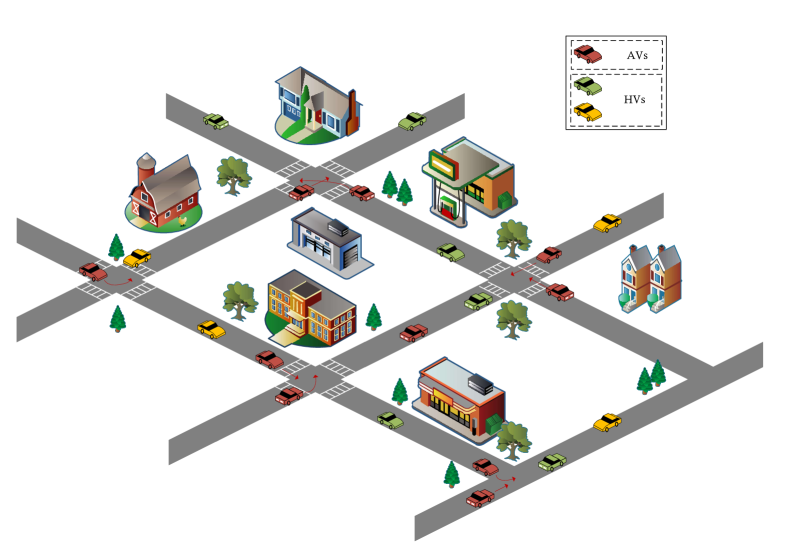
As illustrated in Fig. 1, we consider a mixed autonomy traffic system model with CAVs and some human-driving vehicles (HVs). Consistent with the terminology of parallel MDPs, the state for agent at time-step encompasses information like its velocity , its position , the velocity and relative distance of the vehicles ahead and behind (i.e., ). Meanwhile, each vehicle is controlled by an adjustable target velocity (i.e., ). Furthermore, we assume the dynamics model shall be learned via interactions with the environment. At the same time, the reward function can be calibrated in terms of the velocity and collision-induced penalty, thus being known beforehand.
For simplicity, let be the start time of episode . Within the framework of decentralized multi-agent MBRL, we assume the availability of state transition dataset and each agent approximates by DNNs parameterized by based on historical dataset and exchanged samples from neighbors. In particular, for a time-varying undirected graph constituted by CAVs, each CAV can exchange its latest -length111Notably, the applied length could be episode-dependent but is limited by the maximum value , as will be discussed in Section IV. dataset with neighboring CAVs within the communication range at the end of an episode , where is the dynamic diameter222We slightly abuse the notation of the diameter for an MDP and that for a time-varying undirected graph. of graph . Therefore, when , the multi-agent MBRL problem reverts to parallel single-agent cases. Mathematically, the dataset for dynamics modeling at the end of an episode could be denoted as for all CAV , where the set encompasses all CAVs satisfying with computing the Euclidean distance between CAV and at the last time-step . Furthermore, the planning and control objective for multi-agent MBRL in a communication-limited scenario can be re-written as
| (7) | ||||
where is the learned dynamics model based on . In this paper, we resort to a model-based PETS solution for solving (III-B) and calculating the group regret bound.
IV The MA-PETS Algorithm
In this section, we discuss how to extend PETS [19] to a multi-agent case and present the dynamics model learning and planning & control phases in MA-PETS, which can be depicted as in Fig. 2.
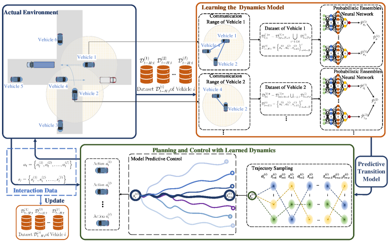
IV-A Learning the Dynamics Model
In MA-PETS, we leverage an ensemble of bootstrapped probabilistic DNNs to reduce both aleatoric and epistemic uncertainty. In particular, in order to combat the aleatoric uncertainty, we approximate the dynamics model at time-step (i.e., ) by a probabilistic DNN, by assuming that the conditioned probability distribution of follows a Gaussian distribution with mean and diagonal covariance parameterized by . In other words,
| (8) |
where denotes a sub-set sampled from and is defined as in (9). Consistent with the definition of states and actions in Section III-B, and .
| (9) | ||||
In addition, in order to mitigate the epistemic uncertainty, which arises primarily from the lack of sufficient data, a PE method is further adopted. Specifically, MA-PETS consists of bootstrap models in the ensemble, each of which is an independent and identically distributed probabilistic DNN from a unique dataset uniformly sampled from with the same size. Typically, [19] points out that yields satisfactory results.
IV-B Planning and Control with Learned Dynamics
Based on a learned dynamics model , MA-PETS tries to obtain a solution to (6) by resorting to a sample-efficiency controller MPC [23]. Generally speaking, MPC avoids cumbersome gradient computation and exhibits strong robustness to the aleatoric and epistemic uncertainty in the learned dynamics model. Without loss of generality, assume that for a time-step , agent observes the state . Afterwards, agent leverages the Cross-Entropy Method (CEM) [44] to generate candidate action sequences within a -horizon of MPC. Initially, each candidate action sequence is sampled following a Gaussian distribution parameterized by . Meanwhile, agent complements possible next-time-step states from the dynamics model ensembles, by adopting particle-based TS [45]. In other words, for each candidate action sequence , TS predicts plausible state-action trajectories by simultaneously creating particles that propagate a set of Monte Carlo samples from the state . Due to the randomness in the learned and assumed time-invariant dynamics model, each particle can be propagated by (), where is a randomly selected dynamics model in the ensemble model. Therefore, the set of plausible state-action trajectories for each candidate action sequence () consists of parallel propagated states with the same action sequence . Afterwards, given the calibrated known reward function , the evaluation of a candidate action sequence can be derived from the average cumulative reward of different parallel action-state trajectories, that is,
| (10) |
After sorting candidate action sequences in terms of the evaluation , elite candidate sequences can be selected to update the Gaussian-distributed sequential decision-making function . Such a TS-based CEM procedure can repeat until convergence of . Therefore, it can yield the desired optimal action sequence satisfying (6) and the MPC controller executes only the first action , transitions the actual environment into the state , and re-calculates the optimal action sequence at the next time-step.
Finally, we summarize our model-based MARL method MA-PETS in Algorithm 1.
Input: communication range , initial state , rarity parameters , max iteration of CEM , accuracy .
V Regret Bound of MA-PETS
Next, we investigate its group regret bound of MA-PETS, by first introducing how to construct an optimistic MDP from a set of plausible MDPs through EVI. Based on that, we derive the group regret bound facilitated by communications within a range of .
V-A EVI for an Optimistic MDP
Beforehand, in order to better exemplify the sample efficiency, we make the following assumptions.
Assumption 1.
The continuous state and action space (i.e., and ) can be quantized. Correspondingly, and denote the size of the discrete state space and action space, respectively.
Assumption 2.
All agents in MA-PETS could enter into the next episode in a “simultaneous” manner, while the episodic length can be tailored to meet some pre-defined conditions.
Assumption 3.
For simplicity of representation, we can scale the reward from to .
Notably, Assumption 1 holds naturally, if we neglect the possible approximation error of DNN in MA-PETS, as it has a trivial impact on understanding the sample efficiency incurred by information exchange. On the other hand, Assumption 2 could be easily met by intentionally ignoring the experienced visits of some “diligent” agents. Moreover, Assumption 3 implies unanimously scaling the group regret bound by , which does not affect learning the contributing impact from inter-agent communications.
Based on these assumptions, we incorporate the concept of a classical MBRL algorithm UCRL2 into the analyses of MA-PETS. In particular, UCRL2 primarily implements the “optimism in the face of uncertainty”, and performs an EVI through episodes , each of which consists of multiple time steps. The term denotes the number of visits to the state-action pair by agent before episode . Next, UCRL2 determines the optimal policy for an optimistic MDP, choosing from a collection of plausible MDPs constructed based on the agents’ estimates and their respective confidence intervals, as commonly governed by the Hoeffding inequality for an agent [46].
Consistent with UCRL2, we allow each agent to enter into a new episode once there exists a state-action pair that has just been played and satisfies . Here denotes the number of state-action visits by agent in the episode and . By Assumption 2, all agents could enter into the next episode in a “simultaneous” manner, by intentionally ignoring the experienced visits of a “diligent” agent after meeting in episode . Therefore, at the very beginning of episode , for each agent , for all state-action pairs . This setting is similar to the doubling criterion in single-agent UCRL2 and ensures that each episode is long enough to allow sufficient learning. Furthermore, different from the single-agent UCRL2, at the end of an episode , consistent with in MA-PETS, each agent has access to all the set of neighboring CAVs , so as to obtain the latest dataset , and constitute . Again, according to Assumption 2, . Afterwards, the EVI proceeds to estimate the transition probability function . In particular, various high-probability confidence intervals of the true MDP can be conjectured according to different concentration inequalities. For example, based on Hoeffding’s inequality [46], the confidence interval for the estimated transition probabilities can be given as
| (11) |
and it bounds the gap between the EVI-conjectured (estimated) transition matrix derived from the computed policy and the empirical average one in episode . Besides, is a pre-defined constant.
Furthermore, a set of plausible MDPs (12) is computed for each agent as
| (12) |
Correspondingly, a policy for an optimistic MDP can be attained from learning in the conjectured plausible MDPs, and then the impact of the communication range on the performance of MA-PETS can be analysed, in terms of the multi-agent group regret in (5).
V-B Analyses of Group Regret Bound
The exchange of information in MA-PETS enhances the sample efficiency, which will be further shown in the derived multi-agent group regret bound. In other words, the difference between single-agent and multi-agent group regret bounds manifests the usefulness of information sharing among agents.
V-B1 Results for Single-Agent Regret Bound
Before delving into the detailed analyses of multi-agent group regret bound, we introduce the following useful pertinent results derived from single-agent regret bound [34].
Consider as a time-homogeneous and communicating MDP with a policy . Meanwhile, by Lemma 1, the optimal -step reward can be approximated by the optimistic average reward . Therefore, if is implemented in for steps, we have the following lemma.
Lemma 2 (Eqs. (7)-(8) of [34]).
Under Lemma 1, the differences between the observed rewards , acquired when agent follows the policy to choose action in state at step , and the aforementioned optimistic average reward forms a martingale difference sequence. Besides, on the basis of Hoeffding’s inequality, with a probability at least , the single-agent bound can be bounded as
| (13) |
where is a constant, and we define the regret in a single episode as that captures the difference between the -step optimal reward and the mean reward with and .
Lemma 2 effectively transforms the cumulative -step regrets into individual episodes of regret. Moreover, the regret bound in Lemma 2 can be classified into two categories, depending on whether the true MDP falls into the scope of plausible MDPs . As for the case where the true MDP is not included in the set of plausible MDPs , the corresponding regret can be bounded by the following lemma.
Lemma 3 (Regret with Failing Confidence Intervals, Eqs. (13) of [35]).
As detailed in Sec. 5.1 of [35], at each step , the probability of the true MDP not being encompassed within the set of plausible MDPs is given by . Correspondingly, the regret attributable to the failure of confidence intervals is
| (14) |
On the other hand, under the assumption that falls within the set , in light of Eq. (8) from [47], we ascertain that due to the approximation error of the EVI,
| (15) |
where represents the optimistic average reward obtained by the optimistically chosen policy , while signifies the actual optimal average reward.
Lemma 4 (Regret with , Sec. 5.2 of [47]).
By the assumption and the gap derived from (15), the regret of agent accumulated in episode could be upper bounded by
| (16) |
where and . Besides, denotes the vector representing the final count of state visits by agent in episode , as determined under the policy , where the operator concatenates the values for all . The are the maximal possible rewards according to a confidence interval similar to (11). is the transition matrix of the policy in the optimistic MDP computed via EVI and typically represents the identity matrix. Furthermore, denotes a modified value vector to indicate the state value range of EVI-iterated episode specific to agent , where and are the state values given by EVI..
As previously noted in Section III-B, we posit that the agents’ reward functions are predetermined, often designed based on task objectives. In line with MA-PETS, the regret contributed by the term (a) in (4) can be disregarded. Therefore, we have the following corollary.
Corollary 1.
By the assumption and the gap derived from (15), the regret of agent accumulated in episode could be upper bounded by
| (17) |
| (18) |
On the other hand, the item (b) (i.e., ) in Lemma 4 (as well as Corollary 1) can be further decomposed and bounded as (18), where, as demonstrated in Eq. (23) of [47], the modified value vector satisfies . In other words, the state value range is bounded by the diameter of the MDP at any EVI iteration. By slight rearrangement of , we have (18), which can be bounded by the following lemma.
Lemma 5 (Eqs. (16)-(17) of [34]).
Contingent on the confidence interval (11), based on our assumption that both and belong to the set of plausible MDPs , the term in (18) can be bounded as
| (19) |
where denotes a constant. Moreover, the term in (18) can be bounded by applying the Azuma-Hoeffding inequality
| (20) |
where denotes a constant.
V-B2 Analysis for Group Regret with Limited-Range Communications
Before analyzing the group regret in the multi-agent system within a constrained communication range, we start with some necessary notations and assume all CAVs constitute a graph. Considering the power graph , which is derived by selecting nodes from the original graph and connecting all node pairs in the new graph that are at a distance less than or equal to a specified value in the original graph. The neighborhood graph represents a sub-graph of , where comprises the set of communication links connecting the agents and . We also define the total number of state-action observations for agent , which is calculated as the sum of observations from its neighbors within the communication range before episode , denoted as . Given the complication to directly estimate , we introduce the concept of clique cover[24] for , which is a collection of cliques that can cover all vertices of a power graph. Further, let denote a clique cover of and a clique . Meanwhile, represents the size of the clique . Additionally, the clique covering number signifies the minimum clique number means finding a minimum number of cliques to cover the power graph within the communication. Furthermore, characterized by a clique covering number , constitutes the clique cover for the graph .
Lemma 6 (Eq. (6) of [38]).
Let represent the clique covering of the graph , where the graph consists of nodes, and the cliques within have node counts . The minimum clique cover maintains a consistent relationship .
In this setup, all agents within a clique explore in proportion to the clique’s size and share the collected samples among themselves. For simplicity, we assume that is connected, meaning that all cliques can communicate with one another. For simplicity, we take to be the number of samples exchanged within the clique before an episode that are available for all agents . In the most challenging scenario, characterized by uniformly random exploration, the algorithm fails to capitalize on any inherent structures or patterns within the environment to potentially refine its learning approach. Consequently, this necessitates a maximum quantity of samples to ascertain an optimal policy, thus giving the worst case. Under these conditions, we present the following lemma.
Lemma 7 (Theorem 1 of [38]).
In the worst case, where the exploration is uniformly random, the number of samples within each clique can be approximated as , where is the maximum horizon, is the number of episodes, and represents the state and action spaces, respectively.
Based on the results of the single-agent regret bound described in Section V-B1, it is ready to analyse the upper bound on the group regret of the multi-agent setting under limited communication range, as shown in Theorem 1.
Theorem 1.
(Hoeffding Regret Bound for Parallel MDP with Limited-Range Communications) With probability at least , it holds that for all initial state distributions and after any steps, the group regret with limited communication range is upper bounded by (21).
| (21) |
Proof.
The proof of Theorem 1 stands consistently with that of Lemma 2. However, it contains significant differences, due to the information exchange-induced distinctive empirical sample size for the transition probabilities.
In particular, the -step group regret in the MDP settings could be bounded based on (5) and (13), that is, by Lemma 2 with a high probability at least ,
| (22) |
As elucidated in Lemma 3, the portion of group regret resulting from failed confidence regions can be bounded by with a probability of at least .
On the other hand, for each episode , under the premise that the true MDP is encompassed within the set of plausible MDPs (), the term is further dissected according to Corollary 1. With Lemma 5, we have
| (23) |
Leveraging the definition that , and applying Jensen’s inequality and the inequality in Lemma 8 in Appendix, we obtain the following results
| (24) |
Furthermore, by Lemma 7, . Thus, we have
| (25) |
where represents the frequency of visits within the clique to a state-action pair after the communications at the end of episode .
Theorem 1 unveils the group regret bound and demonstrates that with respect to , a sub-linear increase in the group regret bound is attained in (21). On the contrary in the standard non-communicative reinforcement learning setting for the same type of algorithm, the group regret is essentially equal to the sum of the single-agent regrets, as implied in Lemma 2.
VI Experimental Settings and Numerical Results
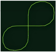
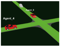
In this section, we evaluate the performance of MA-PETS and demonstrate the superiority of our proposed algorithm over other several state-of-the-art MFRL methods, including PPO [8], DDPG [10], DQN [48], SAC [49]. Specifically, we run our experiments using the CAV simulation platform SMARTS [26] and select the “Unprotected Intersection” scenario in the closed “Figure-Eight” loop, which is a typical mixed autonomy traffic scenario as illustrated in Fig. 3, for the evaluation. We randomly deploy CAVs and a random number of HVs, where the former is controlled by our MA-PETS algorithm and the latter is controlled by the background environment in SMARTS. All CAVs will start from a one-way lane with an intersection, and drive circularly by passing through the intersection and avoiding collisions and congestion. Following the MDP defined in Section III, the corresponding MDP for CAVs in “Unprotected Intersection” is defined as below.
-
•
State and Observation: Except for information about the vehicle itself, each CAV can only observe the information of the vehicle ahead and behind. Hence, it has the information about current state containing the velocity , position of itself, the speed and distance of the vehicles ahead and behind . Hence, as mentioned earlier, the state of vehicle can be represented as .
-
•
Action: As each CAV is only controlled via the target velocity decided by itself, the action of vehicle can be represented as .
-
•
Reward: The goal of CAVs is to maintain a maximum velocity based on no collision. Accordingly, the reward function can be defined as
(26) where the extra term imposes a penalty term on collision, that is, if a collision occurs; and it nulls otherwise.
Notably, given the definition of the reward function in (26), a direct summation of the rewards corresponding to all agents could lead to the computation duplication of some vehicles, thus misleading the evaluation. Therefore, we develop two evaluation metrics from the perspective of system agility and safety. In particular, taking account of the cumulative travel distance of vehicle at time-step and the lasting-time before the collision, we define
| (27) |
and
| (28) |
where () refers to a learned dynamics model until the episode .
| Parameters Description | Settings |
|---|---|
| Number of RL agents | |
| Communication range | |
| Speed per vehicle at time-step | |
| Position per vehicle at | |
| Target velocity per vehicle at | |
| Speed of vehicles ahead and behind | |
| Distance of vehicles ahead and behind | |
| Travel distance per vehicle at | |
| No. of episodes | |
| Maximal length per episode | |
| No. of Ensembles for dynamics Model | |
| Horizon of MPC | |
| Candidate action sequences in CEM | |
| Elite candidate action sequences in CEM | |
| No. of particles | |
| Max iteration of CEM | |
| Proportion of elite candidate action sequences |
In our setting, the number of episodes , while the length of each episode is up to times-steps in case of no collision. We run 5 independent simulations. Besides, typical parameters are summarized in Table II.
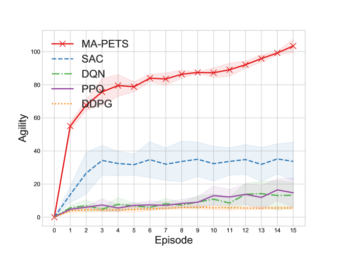
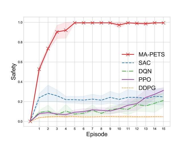
Firstly, we evaluate the performance of MA-PETS for CAVs with communication range and present the performance comparison with MFRL algorithms in Fig. 4. It can be observed from Fig. 4, that our algorithm MA-PETS significantly yields superior outcomes than the others in terms of both agility and safety. More importantly, MA-PETS converges at an apparently faster pace.
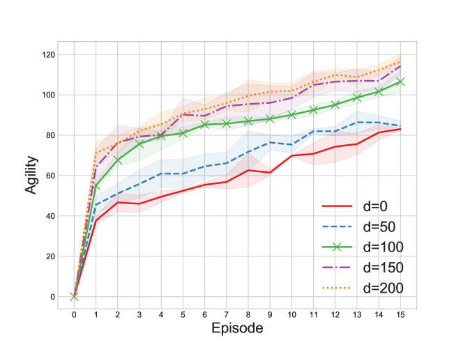
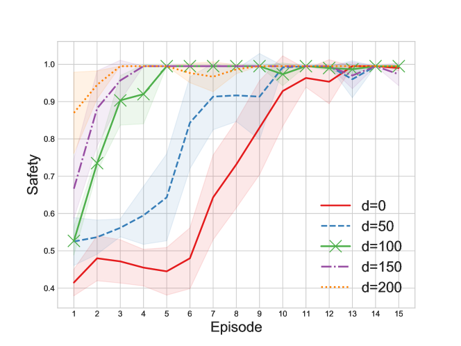
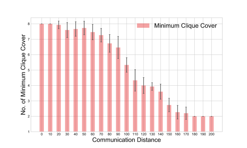
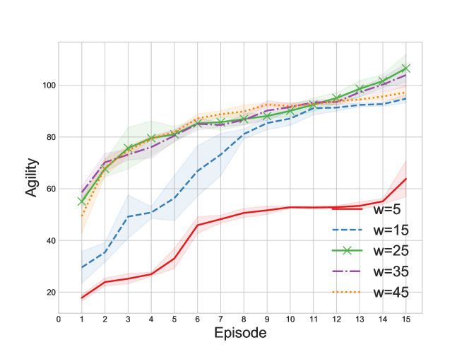
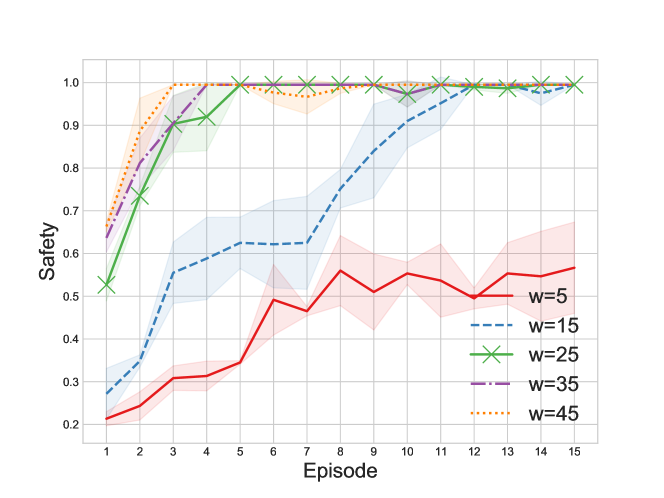
Furthermore, we show the performance of MA-PETS with respect to different values of communication range by varying from to in Fig. 5 and Table III. It can be observed from Table III that consistent with our intuition, the increase in communication range leads to a significant boost of the communications overheads. Meanwhile, as depicted in Fig. 5, it also benefits the learning efficiency of the CAVs is enhanced, thus greatly upgrading the agility and safety. On the other hand, Fig. 5 also unveils that when the communication range increases to a certain extent, a further increase of contributes trivially to the agility and safety of learned policies. In contrast, Table III indicates an exponential increase in the average communications overhead. In other words, it implies a certain trade-off between the learning performance and communication overheads. Consistent with the group regret bound detailed in Section V, we further investigate the numerical interplay between the minimum number of clique covers and communication distance in independent trials. It can be observed from Fig. 6 that while the minimum number of clique covers remains constant beyond a specific communication range threshold, a generally inverse correlation exists between the minimum clique cover number and the communication radius, which aligns with both our theoretical proofs and the experimental findings presented in Fig. 5.
| Name | Value | ||||
|---|---|---|---|---|---|
| Communication Distance | |||||
| Communication Overheads | |||||
To clarify the effect of the MPC horizon in MA-PETS, we perform supplementary experiments in “Figure Eight”. As depicted in Fig. 7, from a security point of view, extending the MPC horizon gradually enhances security. However, beyond a horizon length of , further increases yield only marginal security improvements. In terms of agility, the choice of the MPC horizon is crucial for the performance of the system. In particular, a “too short” horizon introduces a substantial bias in the performance of MA-PETS, as it hampers the ability to make accurate long-term predictions due to the scarcity of time steps. Conversely, a “too long” horizon also results in a noticeable bias. This is due to the increased divergence of particles over extended periods, which reduces the correlation between the currently chosen action and the long-term expected reward. This bias escalates as the horizon increases. Hence choosing an excessively long horizon adversely affects performance.
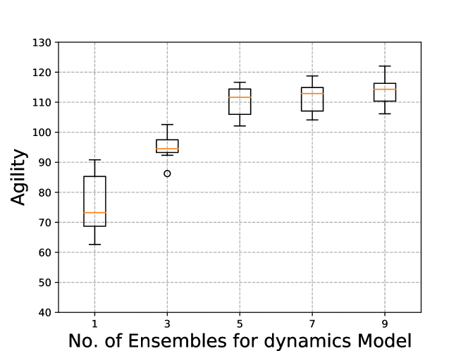
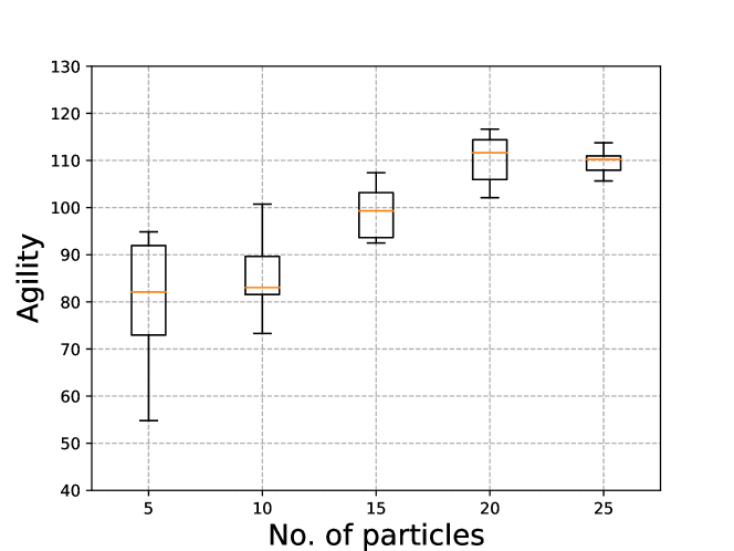
Our research also investigates the influence of the number of ensembles and the number of particles in MA-PETS. In terms of agility, Fig. 8 and Fig. 9 show the corresponding results respectively, which are derived from training episodes through independent simulation runs. It can be observed from Fig. 8 that along with the increase in , the learning becomes more regularized and the performance improves. However, the performance improvement is no longer apparent for a sufficiently large , and this improvement is more pronounced in more challenging and complex environments that require the learning of intricate dynamical models, leaving more scope for effective exploitation of the strategy without the use of model integration. In Fig. 9, superior performance can be reaped for a larger number of particles, due to the fact that more particles allow for a more accurate estimation of the reward for state-action trajectories influenced by transition probabilities.
VII Conclusion and Discussion
In this paper, we have studied a decentralized MBRL-based control solution for CAVs with a limited communication range. In particular, we have proposed the MA-PETS algorithm with a significant performance improvement in terms of sample efficiency. Specifically, MA-PETS learns the environmental dynamics model from samples communicated between neighboring CAVs via PE-DNNs. Subsequently, MA-PETS efficiently develops TS-based MPC for decision-making. Afterwards, we have derived UCRL2-based group regret bounds, which theoretically manifests that in the worst case, limited-range communications in multiple agents still benefit the learning. We have validated the superiority of MA-PETS over classical MFRL algorithms and demonstrated the contribution of communication to multi-agent MBRL.
There are many interesting directions to be explored in the future. For example, we have designed MA-PETS based on a known reward function. However, effective reward design is still an important research topic in the field of RL. Moreover, the ideology of PETS (e.g., ensemble and bootstrap) has been leveraged into many MBRL algorithms, and its integration with the latest DNN solution can be investigated to further improve the performance. Finally, we have only derived the worst case of group regret bound, and the results for more general cases can be explored.
Lemma 8 (Appendix C.3 of [34]).
For any sequence of numbers with , we have
| (29) |
References
- [1] R. Wen, J. Huang, and Z. Zhao, “Multi-Agent Probabilistic Ensembles with Trajectory Sampling for Connected Autonomous Vehicles,” in Proc. IEEE Globecom 2023 (Intelligent6GArch Workshop), Kuala Lumpur, Malaysia, Dec. 2023.
- [2] B. R. Kiran, I. Sobh, V. Talpaert, et al., “Deep reinforcement learning for autonomous driving: A survey,” IEEE Trans. Intell. Transp. Syst., vol. 23, no. 6, pp. 4909–4926, Jun. 2022.
- [3] D. González, J. Pérez, V. Milanés, et al., “A review of motion planning techniques for automated vehicles,” IEEE Trans. Intell. Transp. Syst., vol. 17, no. 4, pp. 1135–1145, Apr. 2016.
- [4] X. Liang, X. Du, G. Wang, et al., “A deep reinforcement learning network for traffic light cycle control,” IEEE Trans. Veh. Technol., vol. 68, no. 2, pp. 1243–1253, Feb. 2019.
- [5] J. Wu, Z. Huang, W. Huang, et al., “Prioritized experience-based reinforcement learning with human guidance for autonomous driving,” IEEE Trans. Neural Netw. Learn. Syst., pp. 1–15, 2022, early Access.
- [6] B. R. Kiran, I. Sobh, V. Talpaert, et al., “Deep reinforcement learning for autonomous driving: A survey,” IEEE Trans. Intell. Transp. Syst., vol. 23, no. 6, pp. 4909–4926, Jun. 2022.
- [7] S. Gronauer and K. Diepold, “Multi-agent deep reinforcement learning: A survey,” Artif. Intell. Rev., vol. 55, no. 2, p. 895–943, Feb. 2022.
- [8] Y. Guan, Y. Ren, S. E. Li, et al., “Centralized cooperation for connected and automated vehicles at intersections by proximal policy optimization,” IEEE Trans. Veh. Technol., vol. 69, no. 11, pp. 12 597–12 608, Sep. 2020.
- [9] J. Zhang, C. Chang, X. Zeng, et al., “Multi-agent DRL-based lane change with right-of-way collaboration awareness,” IEEE Trans. Intell. Transp. Syst., vol. 24, no. 1, pp. 854–869, Jan. 2023.
- [10] R. Lowe, Y. Wu, A. Tamar, et al., “Multi-agent actor-critic for mixed cooperative-competitive environments,” in Proc. Adv. Neural Inf. Proces. Syst. (NIPS), Long Beach, California, USA, Dec. 2017.
- [11] J. N. Foerster, G. Farquhar, T. Afouras, et al., “Counterfactual multi-agent policy gradients,” in Proc. AAAI Conf. Artif. Intell., New Orleans, Louisiana, USA, Feb. 2018.
- [12] T. Rashid, M. Samvelyan, C. S. De Witt, et al., “Monotonic value function factorisation for deep multi-agent reinforcement learning,” J. Mach. Learn. Res., vol. 21, no. 1, pp. 7234–7284, Jan. 2020.
- [13] B. Xiao, R. Li, F. Wang, et al., “Stochastic graph neural network-based value decomposition for marl in internet of vehicles,” IEEE Trans. Veh. Technol., pp. 1–15, 2023, early Access.
- [14] Z. Huang, J. Wu, and C. Lv, “Efficient deep reinforcement learning with imitative expert priors for autonomous driving,” IEEE Trans. Neur. Net. Learn. Syst., vol. 34, no. 10, pp. 7391–7403, Oct. 2023.
- [15] J. Wu, Z. Huang, and C. Lv, “Uncertainty-aware model-based reinforcement learning: Methodology and application in autonomous driving,” IEEE Trans. Intell. Vehicl, vol. 8, no. 1, pp. 194–203, Jan. 2023.
- [16] T. Pan, R. Guo, W. H. Lam, et al., “Integrated optimal control strategies for freeway traffic mixed with connected automated vehicles: A model-based reinforcement learning approach,” Transp. Res. C-Emer. Technol., vol. 123, p. 102987, Feb. 2021.
- [17] A. Der Kiureghian and O. Ditlevsen, “Aleatory or epistemic? Does it matter?” Struct. Saf., vol. 31, no. 2, pp. 105–112, Mar. 2009.
- [18] A. Nagabandi, G. Kahn, R. S. Fearing, et al., “Neural network dynamics for model-based deep reinforcement learning with model-free fine-tuning,” in Proc. IEEE Int. Conf. Rob. Autom. (ICRA), Long Beach, CA, USA, May 2018.
- [19] K. Chua, R. Calandra, R. McAllister, et al., “Deep reinforcement learning in a handful of trials using probabilistic dynamics models,” in Proc. Adv. Neural Inf. Proces. Syst. (NIPS), Montréal, Canada, Dec. 2018.
- [20] A. S. Polydoros and L. Nalpantidis, “Survey of model-based reinforcement learning: Applications on robotics,” J. Intell. Robot. Syst., vol. 86, no. 2, pp. 153–173, May 2017.
- [21] C. Jin, Z. Allen-Zhu, S. Bubeck, et al., “Is q-learning provably efficient?” in Proc. Adv. Neural Inf. Proces. Syst. (NIPS), Montreal, QC, Canada, Dec. 2018.
- [22] Z. Zhang, Y. Zhou, and X. Ji, “Almost optimal model-free reinforcement learningvia reference-advantage decomposition,” in Proc. Adv. Neural Inf. Proces. Syst. (NIPS), Vancouver, BC, Canada, Dec. 2020.
- [23] J. B. Rawlings, “Tutorial overview of model predictive control,” IEEE Contr. Syst. Mag., vol. 20, no. 3, pp. 38–52, Jun. 2000.
- [24] D. Corneil and J. Fonlupt, “The complexity of generalized clique covering,” Discrete Appl. Math., vol. 22, no. 2, pp. 109–118, 1988. [Online]. Available: https://www.sciencedirect.com/science/article/pii/0166218X88900868
- [25] A. Tuynman and R. Ortner, “Transfer in reinforcement learning via regret bounds for learning agents,” Feb. 2022. [Online]. Available: https://api.semanticscholar.org/CorpusID:246473288
- [26] M. Zhou, J. Luo, J. Villella, et al., “SMARTS: An open-source scalable multi-agent rl training school for autonomous driving,” in Proc. Mach. Learn. Res. (PMLR), Cambridge, MA, USA, Nov 2021.
- [27] L. Wei, Z. Li, J. Gong, et al., “Autonomous driving strategies at intersections: Scenarios, state-of-the-art, and future outlooks,” in IEEE Conf. Intell. Transport. Syst. Proc. (ITSC), Indianapolis, IN, United states, Sep. 2021.
- [28] D. Huseljic, B. Sick, M. Herde, et al., “Separation of aleatoric and epistemic uncertainty in deterministic deep neural networks,” in Proc. Int. Conf. Pattern Recognit. (ICPR), Milan, Italy, Jan. 2021.
- [29] M. Deisenroth and C. E. Rasmussen, “PILCO: A model-based and data-efficient approach to policy search,” in Proc. Int. Conf. Mach. Learn. (ICML), Bellevue, Washington, USA, Jun 2011.
- [30] S. Gu, T. Lillicrap, I. Sutskever, et al., “Continuous deep q-learning with model-based acceleration,” in Proc. Int. Conf. Mach. Learn. (ICML), New York, USA, Jun. 2016.
- [31] Y. Guan, Y. Ren, S. E. Li, et al., “Centralized cooperation for connected and automated vehicles at intersections by proximal policy optimization,” IEEE Trans. Veh. Technol., vol. 69, no. 11, pp. 12 597–12 608, Sep. 2020.
- [32] M. Kearns and S. Singh, “Near-optimal reinforcement learning in polynomial time,” Mach. Learn., vol. 49, no. 2, pp. 209–232, Nov. 2002.
- [33] P. Auer and R. Ortner, “Logarithmic online regret bounds for undiscounted reinforcement learning,” in Proc. Adv. Neural Inf. Proces. Syst. (NIPS), Vancouver, BC, Canada, Dec. 2006.
- [34] T. Jaksch, R. Ortner, and P. Auer, “Near-optimal regret bounds for reinforcement learning,” J. Mach. Learn. Res., vol. 11, pp. 1563–1600, Aug. 2010.
- [35] R. Ortner and D. Ryabko, “Online regret bounds for undiscounted continuous reinforcement learning,” in Proc. Adv. Neural Inf. Proces. Syst. (NIPS), Stateline, NV, USA, Dec. 2012.
- [36] I. Osband, D. Russo, and B. Van Roy, “(More) Efficient reinforcement learning via posterior sampling,” in Proc. Adv. Neural Inf. Proces. Syst. (NIPS), Lake Tahoe, Nevada, USA, Dec. 2013.
- [37] B. Hao, Y. Abbasi Yadkori, Z. Wen, et al., “Bootstrapping Upper Confidence Bound,” in Proc. Adv. Neural Inf. Proces. Syst. (NIPS), Vancouver, Canada, Dec. 2019.
- [38] J. Lidard, U. Madhushani, and N. E. Leonard, “Provably efficient multi-agent reinforcement learning with fully decentralized communication,” in Proc. Am. Control Conf. (ACC), Atlanta, GA, USA, Jun. 2022.
- [39] D. S. Bernstein, R. Givan, N. Immerman, et al., “The complexity of decentralized control of markov decision processes,” Math. Oper. Res., vol. 27, no. 4, pp. 819–840, Nov. 2002.
- [40] M. L. Puterman, Markov decision processes: Discrete stochastic dynamic programming. John Wiley & Sons, Apr. 1994.
- [41] P. Gajane, R. Ortner, and P. Auer, “Variational regret bounds for reinforcement learning,” in Proc. UAI 2019, Tel Aviv-Yafo, Israel, May 2019.
- [42] C. B. Browne, E. Powley, D. Whitehouse, et al., “A survey of monte carlo tree search methods,” IEEE Trans. Comp. Intel. AI, vol. 4, no. 1, pp. 1–43, Mar. 2012.
- [43] W. Li and E. Todorov, “Iterative linear quadratic regulator design for nonlinear biological movement systems,” in Lect. Notes Electr. Eng. (ICINCO), Setúbal, Portugal, Aug. 2004.
- [44] Z. I. Botev, D. P. Kroese, R. Y. Rubinstein, et al., “The cross-entropy method for optimization,” in Handbook of statistics, 2013, vol. 31, pp. 35–59.
- [45] A. Girard, C. E. Rasmussen, J. Quinonero-Candela, et al., “Multiple-step ahead prediction for non linear dynamic systems–a gaussian process treatment with propagation of the uncertainty,” in Proc. Adv. Neural Inf. Proces. Syst. (NIPS), Vancouver, British Columbia, Canada, Nov. 2002.
- [46] W. Hoeffding, “Probability inequalities for sums of bounded random variables,” J Am. Stat. Assoc., vol. 58, no. 301, pp. 13–30, 1994.
- [47] R. Ortner, O.-A. Maillard, and D. Ryabko, “Selecting near-optimal approximate state representations in reinforcement learning,” in Lect. Notes Comput. Sci. (LNCS), Bled, Slovenia, May 2014.
- [48] V. Mnih, K. Kavukcuoglu, D. Silver, et al., “Human-level control through deep reinforcement learning,” Nature, vol. 518, no. 7540, pp. 529–533, Feb. 2015.
- [49] T. Haarnoja, A. Zhou, P. Abbeel, et al., “Soft actor-critic: Off-policy maximum entropy deep reinforcement learning with a stochastic actor,” in Proc. Mach. Learn. Res. (PMLR), Stockholm, Sweden, Jul. 2018.