Efficient Quantum Algorithm for Filtering Product States

Abstract

We introduce a quantum algorithm to efficiently prepare states with an arbitrarily small energy variance at the target energy. We achieve it by filtering a product state at the given energy with a Lorentzian filter of width $\delta$. Given a local Hamiltonian on $N$ qubits, we construct a parent Hamiltonian whose ground state corresponds to the filtered product state with variable energy variance proportional to $\delta\sqrt{N}$. We prove that the parent Hamiltonian is gapped and its ground state can be efficiently implemented in $\text{poly}(N,1/\delta)$ time via adiabatic evolution. We numerically benchmark the algorithm for a particular non-integrable model and find that the adiabatic evolution time to prepare the filtered state with a width $\delta$ is independent of the system size $N$. Furthermore, the adiabatic evolution can be implemented with circuit depth $\mathcal{O}(N^{2}\delta^{-4})$. Our algorithm provides a way to study the finite energy regime of many body systems in quantum simulators by directly preparing a finite energy state, providing access to an approximation of the microcanonical properties at an arbitrary energy.

I Introduction

Quantum computing introduces a novel approach to computational tasks, with one of the main advantages being the efficient simulation of physical quantum systems. The advantage lies in the potential for exponential enhancement in spatial resources by encoding the system’s degrees of freedom into qubits, enabling direct operations and calculations on them [1, 2, 3, 4].

A particularly compelling application pertains to determining the ground state properties of systems – a realm of zero-temperature behavior. While, in general, identifying the ground state of a local Hamiltonian stands as a QMA-hard problem [5, 6], for typical physically relevant systems solutions are attainable. Quantum adiabatic evolution offers a method for preparing the ground state of a specified Hamiltonian. This process commences from a readily preparable ground state of the Hamiltonian $H_{0}$ and involves time-evolving the system to a target Hamiltonian $H_{1}$. This strategy’s success relies on an energy gap that scales favorably with system size [7].

Nonetheless, studying excited states is equally important, particularly to understand systems in thermal equilibrium. In practice, addressing a particular eigenstate of the system is extremely difficult. However, analyzing states of a small energy variance around the target energy is equally interesting. Having access to finite energy states of a small energy variance could be useful for studying physics in many fields. In the field of many-body physics, one can calculate the expectation values for observables, perform time dynamics simulations, and calculate entanglement properties of the state, i.e., Renyi entropies [8, 9]. Furthermore, given access to two states at different energies, it becomes possible to verify the predictions of the eigenstate thermalization hypothesis [10]. In chemistry, the excited states can be used to simulate molecular dynamics [11]. The preparation of such states has been well studied using tensor networks [12, 13, 14]. In [13], a relationship between the energy variance and the associated entanglement entropy of the state was established, showing the need for a large bond dimension to approximate the states with small energy variance.

The difficulty of analyzing the excited states classically has sparked an interest in developing quantum algorithms for this purpose. The first quantum algorithm to prepare excited states with reduced variance was quantum phase estimation (QPE) [15, 16]; however, this approach is very costly. An alternative is to use time series [17, 18, 19, 20, 21], which does not require preparation of the state to extract its properties; nevertheless, it uses costly controlled evolution operations. In [22], observables at a given energy were calculated without direct state preparation but through energy filtering with a cosine filter, deconstructing it into a sum of Loschmidt echoes coupled with subsequent classical post-processing.

In this work, we propose a very different way of directly preparing a state of small energy variance. For a given Hamiltonian $H$, we find a product state $\ket{\Psi}$ at the target energy and filter it to an arbitrarily small variance. This is achieved by defining a parent Hamiltonian $\mathcal{H}$ that depends on $H$, $\ket{\Psi}$, and on a filter width parameter $\delta$ that is proportional to the desired energy variance. By construction, the unique ground state $\ket{\Phi}$ of the parent Hamiltonian $\mathcal{H}$ corresponds to the filtered product state. Furthermore, we define a gapped adiabatic path that connects the initial product state $\ket{\Psi}$ with the filtered state $\ket{\Phi}$. Thus, performing adiabatic evolution along this path allows one to efficiently prepare a finite variance approximation of the excited eigenstate at a given energy. We notice that in [23], a similar parent Hamiltonian construction was used to prepare a Gibbs state of a Hamiltonian with commuting terms.

In Section II, we formally introduce the algorithm, in Section III, we perform a numerical investigation to establish tighter bounds to the algorithmic runtime, followed by a summary of our results in Section IV and our conclusions and outlook in Section V.

II Method

II.1 Outline

In this work, we set out to perform the following task. We start with a local Hamiltonian $H$ of interest and a product state $\ket{\Psi}$ that has energy $E_{0}$ and variance $\sigma^{2}_{0}$ with respect to $H$. We want to create a new state $\ket{\Phi}$ that has the same (or close) energy $E_{0}$ but a substantially reduced variance $\sigma^{2}_{\mathcal{L}}$. This is similar to preparing a microcanonical superposition at energy $E_{0}$, just with a finite width. We develop an algorithm that allows us to arbitrarily reduce the variance $\sigma^{2}_{\mathcal{L}}$ in $\text{poly}(N,\delta^{-1})$ time. We achieve this by applying a Lorentzian filter of width $\delta$ on top of the product state $\ket{\Psi}$ (FIG.  1) and suppressing the components of eigenstates with energy far away from $E_{0}$. In the rest of the section, we formally show how this task can be done in a polynomial time, with respect to the system size $N$ and the desired energy variance $\sigma^{2}_{\mathcal{L}}$.

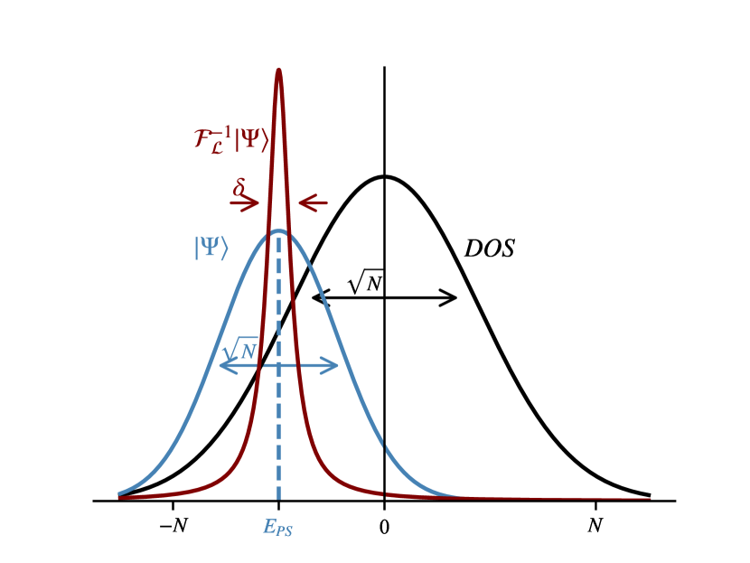
Figure 1: Illustration of the filtering. The figure shows the density of states (DOS) for the Hamiltonian $H$ and the product state $\ket{\Psi}$. The red line shows the process of applying the Lorentzian filter $\mathcal{F}^{-1}_{\mathcal{L}}$ onto the product state $\ket{\Psi}$, which leads to a state of reduced energy variance.

The algorithm informally proceeds as follows:

1. Start with a product state $\ket{\Psi}$, at the desired energy $E_{0}$. Define projectors $P_{i}$ on each site $i$ that annihilate the state $\ket{\Psi}$. The sum of these projectors $P=\sum_{i}P_{i}$ defines a Hamiltonian whose ground state is the product state (see Lemma II.1).

2. Pick the width $\delta$ of the Lorentzian filter to be applied to $\ket{\Psi}$.

3. Construct the parent Hamiltonian:

   $$\mathcal{H}(E_{0},\delta)=\sum_{i}\mathcal{F}_{\mathcal{L}}^{\dagger}P_{i}\mathcal{F}_{\mathcal{L}},$$

   $$\text{where}\quad\mathcal{F}_{\mathcal{L}}=(1+i\delta^{-1}(H-E_{0})).$$

   The parent Hamiltonian $\mathcal{H}$ has a unique ground state that corresponds to the filtered state (Lemma II.1), and it remains gapped (Lemma II.2).

4. Prepare the filtered state $\ket{\Phi}$ by adiabatically evolving the product state $\ket{\Psi}$ with $\mathcal{H}(\delta)$ by slowly increasing $\delta^{-1}(s)=s\delta^{-1}$ from $s=0$ to $1$. In Lemma II.3, we show that the adiabatic evolution time is $T=\text{poly}(N,\delta^{-1})$. Note that $\mathcal{H}(s=0)=P$. In Lemma B, we address the circuit depth required for Trotterized time evolution.

5. By choosing a suitable $\delta$, we can thus prepare a filtered product state of arbitrary energy variance. In Lemma II.4, we discuss how the variance of the filtered state decreases with $\delta$ in the thermodynamic limit.

II.2 The algorithm

Let $H$ be a local Hamiltonian of interest with eigenbasis $H\ket{e_{n}}=e_{n}\ket{e_{n}}$ and $\ket{\Psi}$ be a product state for which we can define local projectors $P_{i}$ that annihilate it. Let the energy of the product state be $E_{0}$. We set out to prepare the filtered state $\ket{\Phi}$, corresponding to filter $\mathcal{F}_{\mathcal{L}}$. This state is given by $\ket{\Phi}\propto\mathcal{F}^{-1}_{\mathcal{L}}\ket{\Psi}$. In this paper, we will use the Lorentzian filter $\mathcal{F}_{\mathcal{L}}$; however, the strategy works for any filter that is polynomial in $H$. The Lorentzian filter is given by

$$\mathcal{F}_{\mathcal{L}}(E,\delta)=(1+i\delta^{-1}(H-E)),$$ (1)

with the corresponding filtered state :

$$\ket{\Phi}\propto\mathcal{F}^{-1}_{\mathcal{L}}\ket{\Psi}=\sum_{n}\frac{c_{n}}{1+i\delta^{-1}(e_{n}-E)}\ket{e_{n}},$$ (2)

$$\absolutevalue{\bra{e_{n}}\ket{\Phi}}^{2}\propto\frac{\absolutevalue{c_{n}}^{2}}{1+\delta^{-2}(e_{n}-E)^{2}}.$$ (3)

Note that the probability amplitude of $\ket{e_{n}}$ has been suppressed here by a Lorentzian factor $\frac{\absolutevalue{c_{n}}^{2}}{1+\delta^{-2}(e_{n}-E)^{2}}$.

For a filter $\mathcal{F}_{\mathcal{L}}$ and initial state $\ket{\Psi}$ we can define the parent Hamiltonian $\mathcal{H}$:

$$\mathcal{H}=\sum_{i}\mathcal{F}^{\dagger}_{\mathcal{L}}P_{i}\mathcal{F}_{\mathcal{L}}.$$ (4)

Note that for a local Hamiltonian $H$, the operator norm of the parent Hamiltonian scales as $\norm{\mathcal{H}}=\mathcal{O}(N^{3}\delta^{-2})$. We take this scaling into account when establishing the bounds for the runtime and circuit depth. In the rest of the section, we formally show that by finding the ground state of $\mathcal{H}$, we obtain the filtered state $\ket{\Phi}$ and that one can achieve this task in a polynomial time on a quantum computer.

Lemma II.1.

Let $H$ be an arbitrary, k-local many body Hamiltonian, $\ket{\Psi}$ the initial product state and $\sum_{i=1}^{N}P_{i}$ a sum of local, commuting projectors satisfying $P_{i}$, $\commutator{P_{i}}{P_{j}}=0,P_{i}\ket{\Psi}=0\quad\forall i,j$. Let $E$ and $\delta$ be the center and width of the filter $\mathcal{F}^{-1}(E,\delta)$, respectively. Then $\mathcal{H}=\mathcal{F}^{\dagger}\left(\sum_{i=1}^{N}P_{i}\right)\mathcal{F}$ is a parent Hamiltonian whose unique ground state is the filtered state $\ket{\mathrm{GS}}_{\mathcal{H}}=\frac{1}{\mathcal{N}}\mathcal{F}^{-1}(E,\delta)\ket{\Psi}$, where $\mathcal{N}$ is a normalization constant

Proof.

The unique ground state of $\sum_{i=1}^{N}P_{i}$ is the initial state $\ket{\Psi}$ with a ground state energy 0, by construction. Note that $\mathcal{H}$ is a sum of positive semi-definite terms since:

$$\mathcal{F}^{\dagger}P_{i}\mathcal{F}=\mathcal{F}^{\dagger}P_{i}P_{i}\mathcal{F}=r_{i}^{\dagger}r_{i}\quad\text{where}\quad r_{i}\equiv P_{i}\mathcal{F},$$ (5)

thus the ground state of the parent Hamiltonian $\mathcal{H}$ has energy $E\geq 0$. Furthermore, note that, by construction,

$$P_{i}\ket{\Psi}=P_{i}\mathcal{F}\mathcal{F}^{-1}\ket{\Psi}=\mathcal{F}^{\dagger}P_{i}\mathcal{F}\mathcal{F}^{-1}\ket{\Psi}=0.$$ (6)

Hence the parent Hamiltonian $\mathcal{H}$ has ground state:

$$\ket{\mathrm{GS}}_{\mathcal{H}}=\frac{1}{\mathcal{N}}\mathcal{F}^{-1}\ket{\Psi}=\ket{\Phi},$$ (7)

with ground state energy 0. Therefore,

$$0 =\left(\sum_{i=1}^{N}P_{i}\right)\ket{\Psi}=\left(\sum_{i=1}^{N}P_{i}\right)\mathcal{F}\mathcal{F}^{-1}\ket{\Psi},$$

and thus,

$$\mathcal{H}\mathcal{F}^{-1}(E,\delta)\ket{\Psi}=\mathcal{F}^{\dagger}\left(\sum_{i=1}^{N}P_{i}\right)\mathcal{F}\mathcal{F}^{-1}\ket{\Psi}=0,$$ (8)

where the normalized ground state is given by: $\ket{\mathrm{GS}}_{\mathcal{H}}=\frac{1}{\mathcal{N}}\mathcal{F}^{-1}(E,\delta)\ket{\Psi}$, which corresponds to the filtered state $\ket{\Phi}$. ∎

Next, we prove that the parent Hamiltonian $\mathcal{H}$ is gapped.

Lemma II.2.

The parent Hamiltonian $\mathcal{H}$ is gapped with a gap $\Delta\geq 1$ for a filter satisfying $\mathcal{F}^{\dagger}\mathcal{F}\succeq 1$.

Proof.

We use the martingale method [24] to prove that $\mathcal{H}$ is gapped; in particular, we show that $\mathcal{H}^{2}-\Delta\mathcal{H}\succeq 0$ for a gap of $\Delta=1$.

$$\mathcal{H}^{2}-\mathcal{H}=$$

$$=\mathcal{F}^{\dagger}\left(\sum_{i=1}^{N}P_{i}\right)\mathcal{F}^{\dagger}\mathcal{F}\left(\sum_{i=1}^{N}P_{i}\right)\mathcal{F}-\mathcal{F}^{\dagger}\left(\sum_{i=1}^{N}P_{i}\right)\mathcal{F}$$

$$=\mathcal{F}^{\dagger}\left(\sum_{i=1}^{N}P_{i}\right)\mathcal{F}^{\dagger}\mathcal{F}\left(\sum_{i=1}^{N}P_{i}\right)\mathcal{F}-\mathcal{F}^{\dagger}\left(\sum_{i=1}^{N}P^{2}_{i}\right)\mathcal{F}$$

$$\succeq\mathcal{F}^{\dagger}\left(\sum_{i=1}^{N}P_{i}\right)\mathcal{F}^{\dagger}\mathcal{F}\left(\sum_{i=1}^{N}P_{i}\right)\mathcal{F}-\mathcal{F}^{\dagger}\left(\sum_{i=1}^{N}P_{i}\right)^{2}\mathcal{F}$$

$$=\mathcal{F}^{\dagger}\left(\sum_{i=1}^{N}P_{i}\right)(\mathcal{F}^{\dagger}\mathcal{F}-1)\left(\sum_{i=1}^{N}P_{i}\right)\mathcal{F}$$

$$=V^{\dagger}(\mathcal{F}^{\dagger}\mathcal{F}-1)V$$

$$\succeq 0,$$

since $(\mathcal{F}^{\dagger}\mathcal{F}-1)\succeq 0$, where $V=\left(\sum_{i=1}^{N}P_{i}\right)\mathcal{F}$. ∎

In the following Lemma II.3, we combine the results to show that the algorithm has a polynomial run time.

Lemma II.3.

Provided that the parent Hamiltonian $\mathcal{H}$ is k-local, we can prepare the ground state $\ket{\Phi}=\frac{1}{\mathcal{N}}\mathcal{F}^{-1}(E,\delta)\ket{\Psi}$, hence perform the filtering, in time $T=\text{poly}(N,\delta^{-1})$ and consequently with circuit depth $D=\text{poly}(N,\delta^{-1})$.

The proof is given in the Appendix A.

In Lemma II.4, we establish the relationship of the obtained energy variance $\sigma^{2}_{\mathcal{L}}$ and the Lorentzian filter width $\delta$.

Lemma II.4.

Let $H$ be a local Hamiltonian on $N$ qubits, $\ket{\Psi}$ the initial product state, and $\mathcal{F}_{\mathcal{L}}$ the Lorentzian filter with parameters $E$, $\delta$. If the filter energy is $E=\bra{\Psi}H\ket{\Psi}$, then the variance of the filtered state is $\sigma^{2}_{\mathcal{L}}\approx\delta\sqrt{2\sigma^{2}_{0}/\pi}$, in the limit where $\delta/\sqrt{\sigma^{2}_{0}}<<1$.

See Appendix C for the proof and the exact variance dependence.

The above results prove that the filtering of a product state with a Lorentzian filter can be achieved in $\text{poly}(N,\delta^{-1})$ time.

II.3 Product State remarks

For a product state $\ket{\Psi}$ with regards to the energy eigenbasis of a local Hamiltonian $H=\sum_{j}h_{j}$, the variance scales as:

$$\sigma^{2}_{0}=\bra{\Psi}H^{2}\ket{\Psi}-\bra{\Psi}H\ket{\Psi}^{2}=\mathcal{O}(N),$$ (9)

where $E_{0}=\bra{\Psi}H\ket{\Psi}$. Furthermore, $E_{0}$ and the initial variance $\sigma^{2}_{0}$ can be easily computed classically. If the filter energy $E$ is chosen to be the product state energy $E_{0}=\bra{\Psi}H\ket{\Psi}$, provably successful energy filtering of the product state $\ket{\Psi}$ can be achieved.

For any product state $\ket{\Psi}=\otimes_{i}\ket{\phi_{i}}$ we can always create the projectors $P_{i}$ acting on a single qubit by $P_{i}=\mathbb{I}-\ket{\phi_{i}}\bra{\phi_{i}}$. For a local $H$, product states span an extensive energy range [25]. For a target energy within that range, it is then possible to prepare a state with a small energy variance on a quantum computer. Note that our runtime guarantees are provable only when we filter around the product state energy $E_{0}$. This arises from the fact that the Lorentzian and Gaussian functions decay at different speeds. Thus, if we pick $E\neq E_{0}$, the final energy $\bra{\Phi}H\ket{\Phi}$ can differ from the filter energy $E$.

III Results

In the previous sections, we have shown that the Lorentzian filtering can be done in a polynomial time by adiabatic evolution since the gap of the parent Hamiltonian $\mathcal{H}$ does not close throughout the evolution. However, the bounds on the adiabatic runtime are often loose, and in practice, one requires a much shorter runtime. We numerically benchmark the algorithm to show that we already observe a good agreement with theory for moderate system sizes $N$ and show that the algorithm requires a significantly shorter adiabatic evolution time. For the numerical results, we use the Transverse Field Ising (TFI) Hamiltonian $H$

$$H=J\left(\sum_{i=1}^{N-1}Z_{i}Z_{i+1}+\sum_{i=1}^{N}gX_{i}+hZ_{i}\right),$$ (10)

with coefficients $(J,g,h)=(1,-1.05,0.5)$, far away from integrability. The $(X_{i},Z_{i})$ denotes the respective Pauli matrix on site $i$. We consider two types of initial product states $\ket{\Psi}$. Firstly, the antiferromagnetic (AFM) state $\ket{\text{AFM}}=\ket{101\dots}$. Secondly, we look at a family of translationally invariant product states of the form $\ket{p(\theta)}=(\cos(\theta)\ket{0}+\sin(\theta)\ket{1})^{\otimes N}$. In principle, varying $\theta$ allows us to cover an extensive range of energies (see Appendix D). While in the thermodynamic limit, the product states have a Gaussian eigenstate distribution, for small systems, the distribution can differ. We investigate the case for $\theta=\pi/6$ as the state lies closer to the center of the spectrum, where the density of states is larger, and has an eigenstate distribution closer to the Gaussian one. We expect this to give a better agreement with the theory for small systems.

For a given product state $\ket{\Psi}$, we create the projectors $P_{i}$ on each site that annihilate it. We proceed to investigate the parent Hamiltonian:

$$\mathcal{H}=(1-\frac{i}{\delta}(H-E_{F}))\left(\sum_{i=1}^{N}P_{i}\right)(1+\frac{i}{\delta}(H-E_{F})).$$ (11)

In this section, we show numerical results obtained with exact diagonalization for system sizes up to $N=18$ sites. Reaching larger system sizes with a classical simulation proves to be a computationally prohibitive task. In particular, since we are targeting states in the middle of the spectrum, the entanglement entropy is expected to scale as a volume law, preventing a systematic exploration with matrix product state methods [26], as we discuss more in detail in Appendix E.

III.1 Expected decrease of the energy variance

Here, we numerically investigate the ground state of $\mathcal{H}$ corresponding to the filtered product state. In particular, we investigate how the variance $\sigma^{2}_{\mathcal{L}}$ of the Lorentzian-filtered state depends on the parameter $\delta$ for various system sizes $N$. In Lemma II.4, we derive the relationship between variance and $\delta$. For low $\delta$ values, this relationship reduces to:

$$\sigma^{2}_{\mathcal{L}}/\sqrt{\sigma^{2}_{0}}=\delta\sqrt{2/\pi}.$$ (12)

In Fig. 2, we consider the decay of the variance for the AFM initial state, which lies at the edge of the spectrum of the Hamiltonian $H$. Fig. 3 correspondingly shows the results for the initial state $\ket{p(\theta=\pi/6)}$, which lies more toward the center of the spectrum. We observe a good agreement with theory in both cases, with a better agreement for the small system sizes in the case of $\ket{p(\theta=\pi/6)}$ initial state.

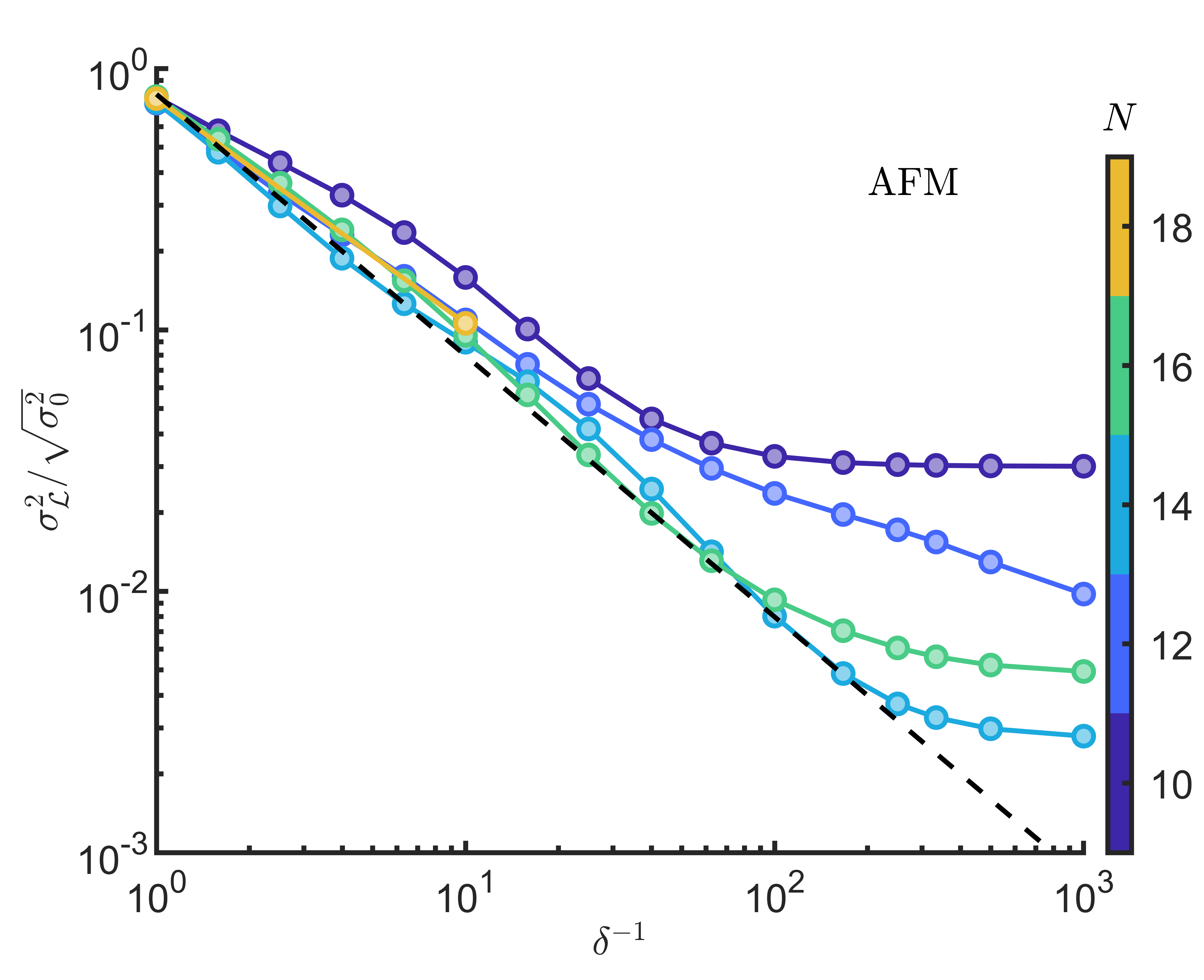
Figure 2: The figure shows, for various system sizes $N$, the performance of the filter applied on the AFM product state at the mean energy which, in the thermodynamic limit, corresponds to energy density $E_{0}/JN=1$. The black line shows the expected variance decay (Eq. 12).

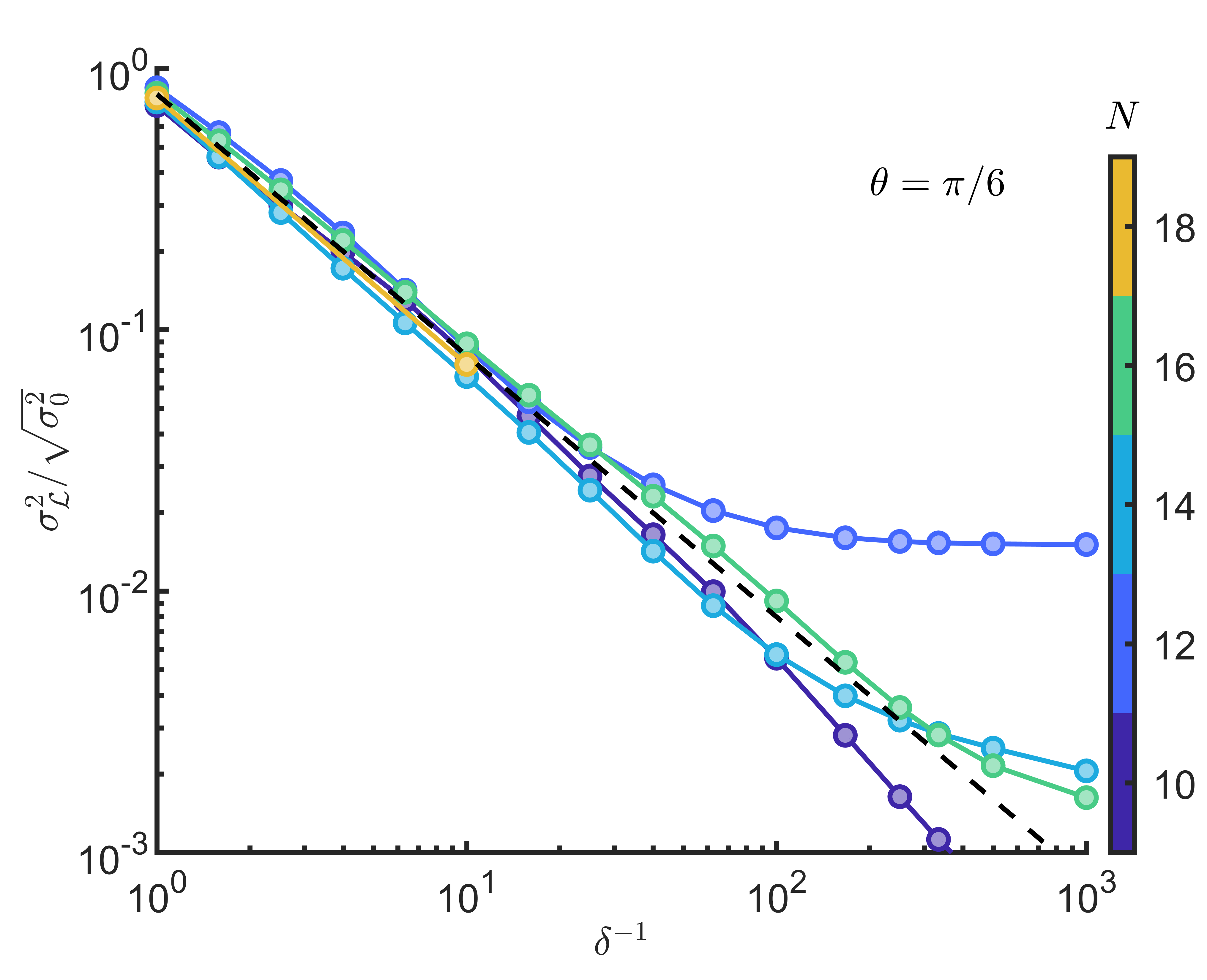
Figure 3: The figure shows, for various system sizes $N$, the performance of the filter applied on the $\ket{p(\theta=\pi/6)}$ product state at the mean energy which, in the thermodynamic limit, corresponds to energy density $E_{0}/JN=-0.409$. The black line shows the expected variance decay (Eq. 12).

III.2 Adiabatic Evolution

To better understand the actual adiabatic runtime $T$ required, we numerically investigate the performance of the adiabatic evolution in practice. On a quantum device, one could prepare the filtered state by time evolving the product state with $\mathcal{H}(\delta)$ while smoothly increasing $\delta^{-1}$ from 0 to the desired value. In particular, for this study, we choose the adiabatic scheduling $\delta^{-1}(s)=\sin(\pi/2\sin(s\pi/2)^{2})^{2}\delta^{-1}_{\max}$ which ensures a slower change of the parameter at the beginning and end of the evolution. This scheduling of the adiabatic evolution is essential for an optimal runtime [27].

To investigate the accuracy of the adiabatic evolution for various system sizes, we study the fidelity of the adiabatic state $\mathcal{F}$ with respect to the exact filtered state and monitor the ground state energy of the parent Hamiltonian $\mathcal{H}$ since, for perfectly adiabatic evolution, it should remain zero throughout. Note that the parent Hamiltonian $\mathcal{H}$ (Eq. 11) has a norm that increases with $\delta^{-1}$. To keep it normalized throughout adiabatic evolution, we rescale it to $\tilde{\mathcal{H}}(\delta)=\mathcal{H}(\delta)/(1+\delta^{-2})$. Note that the rescaling affects the gap, which we take into account when establishing the runtime. We apply the adiabatic evolution in the following way:

$$\ket{\Phi}_{\mathrm{adi}}=\prod_{l=1}^{T/\tau}\exp(-i\tau\tilde{\mathcal{H}}\{\delta(l\frac{\tau}{T})\})\ket{\Psi},$$ (13)

where $\tau$ is the discrete adiabatic time step, and $T$ is the total adiabatic evolution time. To benchmark the adiabatic evolution, we fix the desired filter width to be $\delta=0.1$ and perform the evolution for several system sizes $N$ and runtimes $T$. In Fig. 4 and Fig. 5, we show the dependence of the fidelity $\mathcal{F}$ and the parent Hamiltonian $\mathcal{H}$ energy with respect to the adiabatic evolution time $T$. In both cases, the parent Hamiltonian $\mathcal{H}$ energy appears independent of the system size, while the fidelity shows a favorable behavior towards larger $N$. These results provide a more favorable scaling for the adiabatic runtime $T$ compared to the adiabatic theorem, which suggests that $T=\mathcal{O}(N^{3})$. The results suggest that the adiabatic evolution runtime could be taken independently of the system size to prepare the state with a given fidelity $\mathcal{F}$. However, in Appendix B, we show that the circuit depth required to implement this evolution via the first-order Trotterization scales as $\mathcal{O}(N^{2})$ since $\norm{\mathcal{H}}=\mathcal{O}(N^{3})$.

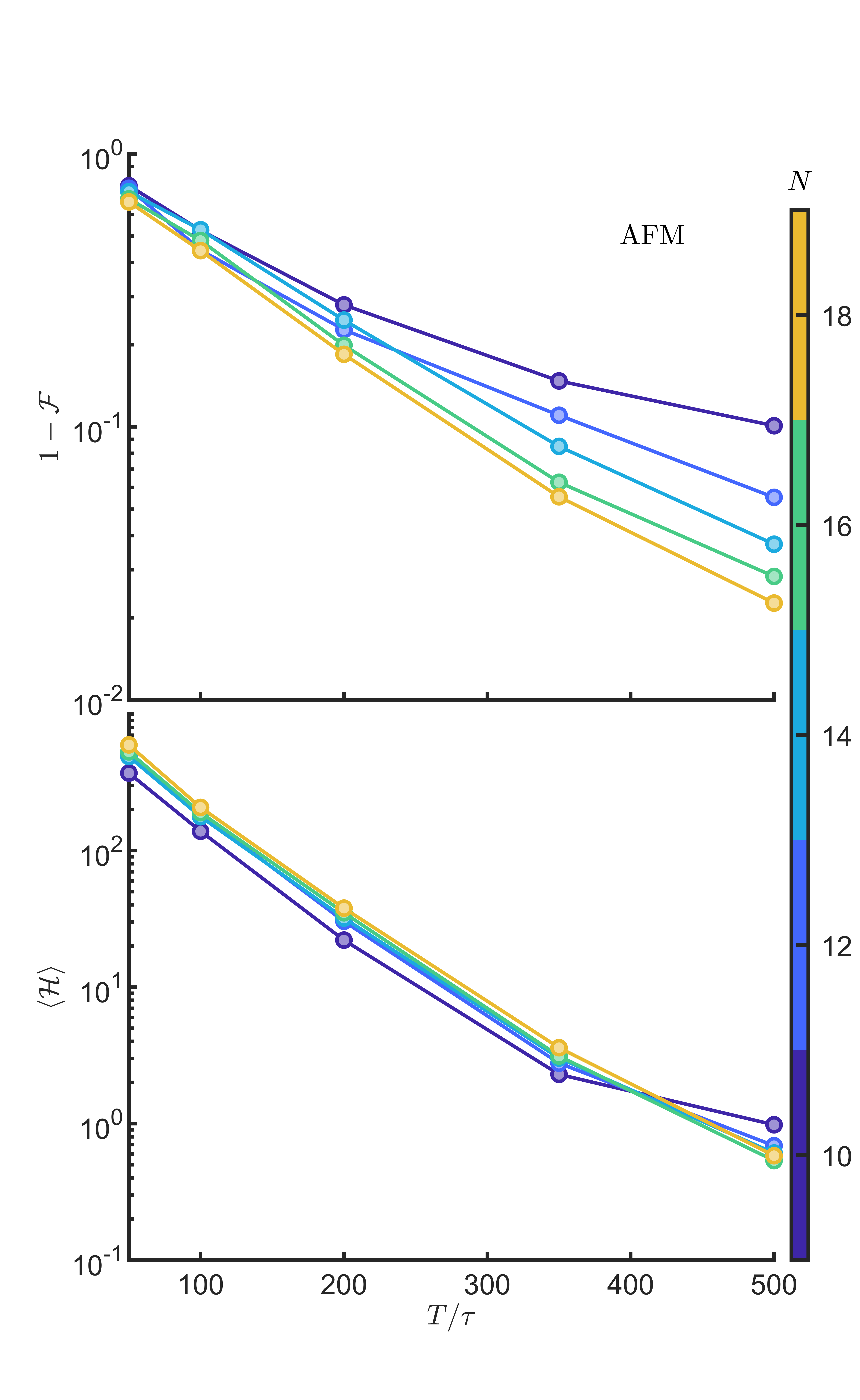
Figure 4: The figure shows results for adiabatic evolution of the $\ket{AFM}$ initial product state for final filter width $\delta=0.1$ and several system sizes $N$. We use $\tau=0.1$. The upper plot shows one minus the fidelity between the evolved state and the exact filtered one as a function of the number of timesteps $T/\tau$. The lower plot shows the parent Hamiltonian $\mathcal{H}$ energy at the end of the adiabatic evolution.

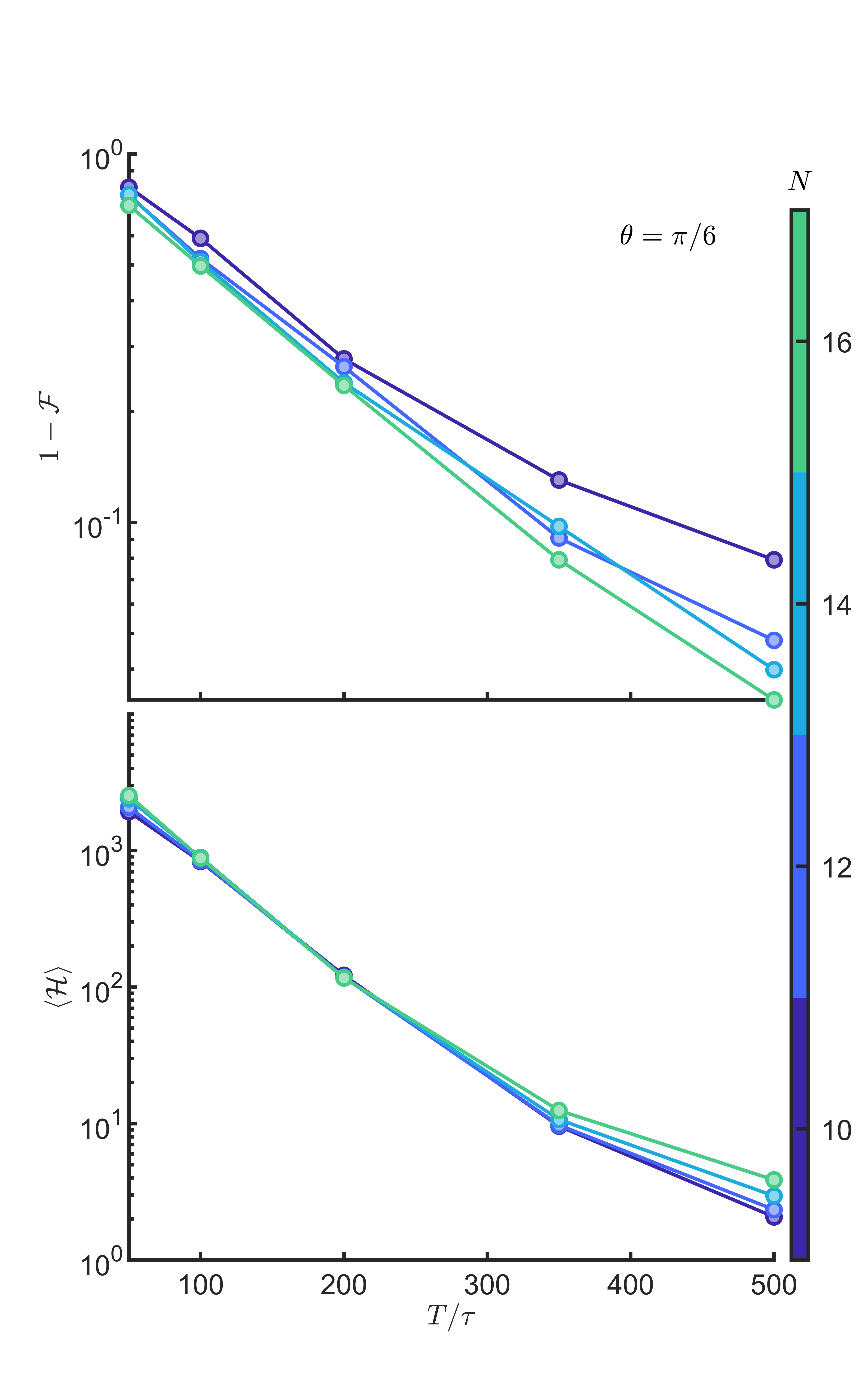
Figure 5: The figure shows results for adiabatic evolution of $\ket{p(\theta=\pi/6)}$ initial product state for final filter width $\delta=0.1$ and various system sizes $N$. We use $\tau=0.1$. The upper plot shows one minus the fidelity between the evolved state and the exact filtered one as a function of the number of timesteps $T/\tau$. The lower plot shows the parent Hamiltonian $\mathcal{H}$ energy at the end of the adiabatic evolution.

IV Discussion

In this section, we review the results from Section III and discuss the behavior and drawbacks of the Lorentzian filtering for finite system sizes.

Firstly, Fig. 2 and Fig. 3 show that, even for small system sizes $N$, the variance of the filtered state follows the decreasing behavior expected in the thermodynamic limit (Eq. 12). In the numerics, we observe that the smaller systems start to deviate from this behavior first. The first reason for this behavior is that the eigenstate distribution of the product state is not Gaussian for small systems. The second reason is the discreteness of the spectrum. In Eq. (3), we establish that the suppression due to Lorentzian filtering is given by $\frac{\absolutevalue{c_{n}}^{2}}{1+\delta^{-2}(e_{n}-E)^{2}}$. Suppose that the closest eigenstate is $\eta=\min_{n}{\absolutevalue{e_{n}-E}}$ away from the center of the filter. It is clear that further lowering $\delta$ leads to no further filtering when $\delta^{-1}\eta\gtrsim 1$. However, for larger systems, the discreteness of the spectrum should not pose any problems. Note that for a Hamiltonian $H$ on $N$ sites, the energy extent is $O(N)$, while there are $2^{N}$ eigenstates. This means that the density of states, along with the number of states supported by the product state, increases exponentially with $N$, and thus $\eta$ becomes exponentially small in $N$. The exponential density of states allows for successful filtering to be performed up to exponentially small $\delta$ values.

Secondly, in Fig. 4 and Fig. 5, we observe that the adiabatic runtime required to reach a certain precision is essentially independent of the system size $N$. Even though the fidelity is only accessible in exact calculations, measuring the energy of the parent Hamiltonian $\mathcal{H}$ at the end of the evolution, as seen in the figures, provides a reliable indication that the adiabatic evolution has indeed prepared the required state. The numerics indicate that the runtime of the algorithm is much faster than expected, and one can prepare a state of given $\delta$ with a fixed number of Trotter steps that are independent of $N$.

Thirdly, perhaps the biggest drawback of the proposed algorithm is the fact that it requires evolving the system under a geometrically non-local Hamiltonian. Whereas this would, in principle, be possible on some platforms, like trapped ions [28], on other quantum computer implementations with only local gates available, it would require $\mathcal{O}(N)$ additional swap operations, which will increase the cost of the algorithm and, potentially, render it unsuitable for NISQ devices. This is, however, not surprising when considering that the states we are trying to filter are excited eigenstates of the Hamiltonian, which usually exhibit an entanglement volume law [29, 30, 31], and thus cannot be encoded, in general, in the ground state of a geometrically local Hamiltonian (which would only accommodate area law entanglement).

V Conclusion

We have developed a novel algorithm for preparing states with an arbitrarily small energy variance at a target energy on a quantum computer. The algorithm effectively prepares a state that would result from applying a Lorentzian filter of width $\delta$ to an initial product state. The filtered state is, in fact, adiabatically prepared as the ground state of a parent Hamiltonian. Furthermore, we prove that the algorithm is efficient since the parent Hamiltonian remains gapped with a gap independent of system size; thus, it can be efficiently prepared with adiabatic evolution. Indeed, the running time of the algorithm is polynomial both in the system size and the inverse width.

We show that when preparing the finite energy state, its variance decreases with the parameter $\delta$ that defines the Lorentzian filter, and already for moderate system sizes, we observe good agreement with the asymptotic predictions for large sizes. While according to the theoretical bounds, the adiabatic runtime scales as $O(N^{3}\delta^{-4})$, our numerics suggest that in practice, the required time is much more favorable due to the looseness of the theoretical bound from the adiabatic theorem. In practice, we estimate that the adiabatic runtime scales as $O(\delta^{-4})$, thus allowing us to perform adiabatic evolution and prepare the finite energy state with circuit depth $O(N^{2}\delta^{-4})$ (see Appendix B).

Our approach provides a new way of probing finite energy physics on quantum devices by directly giving access to small energy variance states. Having access to the state itself provides novel ways to probe finite energy regimes of isolated quantum systems and allows this algorithm to serve as a subroutine in more complicated analysis on quantum devices. Future work should focus on developing new algorithms that take advantage of the access to filtered product states.

Appendix A Adiabatic runtime

In this appendix we discuss the adiabatic runtime and prove Lemma II.3.

Proof.

The adiabatic theorem states that if the adiabatic evolution is slow enough and the state is gapped then the system will remain in the instantaneous ground state of the Hamiltonian $H(s)$. The result from [32, 27, 33] states that the required runtime for the adiabatic evolution is:

$$T\geq\max_{s}(\norm{\dot{H}(s)}/\Delta(s)^{2}),$$ (14)

where we smoothly vary the parameter $s$ from $0$ to $1$. To keep the norm of the parent Hamiltonian independent of $\delta^{-1}$ throughout the adiabatic evolution, we rescale it as follows:

$$\tilde{\mathcal{H}}(s) =\frac{1}{1+s^{2}\delta^{-2}}V\left(\sum_{i=1}^{N}P_{i}\right)V^{{\dagger}},\quad\text{where}$$

$$V =\left(1+is\delta^{-1}(H-E)\right).$$

When rescaled in this way from Lemma II.2 one can clearly see that the gap $\Delta(s)\geq\frac{1}{1+s^{2}\delta^{-2}}$. Furthermore, by differentiating $\tilde{\mathcal{H}}(s)$ with respect to $s$ we obtain that:

$$\dot{\tilde{\mathcal{H}}}(s) =\frac{-2s\delta^{-2}}{(1+s^{2}\delta^{-2})^{2}}V\left(\sum_{i=1}^{N}P_{i}\right)V^{{\dagger}}$$

$$+\frac{1}{1+s^{2}\delta^{-2}}(\dot{V}\left(\sum_{i=1}^{N}P_{i}\right)V^{\dagger}+V\left(\sum_{i=1}^{N}P_{i}\right)\dot{V}^{{\dagger}})$$

$$=\frac{1}{1+s^{2}\delta^{-2}}(-2s\delta^{-2}\mathcal{H}(s)$$

$$+\delta^{-1}(i(H-E)\left(\sum_{i=1}^{N}P_{i}\right)V^{\dagger}+h.c.)$$

$$=O(N^{3}),$$

since $\norm{V}=\mathcal{O}(\delta^{-1}N)$ and $\norm{H}=\mathcal{O}(N)$ Combining the previous bound for $\norm{\dot{\tilde{\mathcal{H}}}(s)}$ and the scaling of the gap $\Delta(s)$ we arrive at the adiabatic runtime:

$$T \geq\max_{s}(\norm{\dot{\tilde{\mathcal{H}}}(s)}/\Delta(s)^{2})$$

$$=O(N^{3}\delta^{-4}),$$

which gives the $T=\text{poly}(N,\delta)$ adiabatic runtime.

Secondly, we use the fact that the time evolution on quantum computers can be performed efficiently for a local Hamiltonian $H=\sum_{\gamma=1}^{M}h_{\gamma}$ using any of the algorithms [34, 35, 36]. Thus, the evolution can be simulated with a $\text{poly}(N,\delta)$-depth quantum circuit. In Appendix B, we explicitly show the depth required to implement the first-order Trotter evolution. ∎

Appendix B Trotter Circuit depth for the adiabatic evolution

This appendix shows that the first-order Trotterized time evolution of $\mathcal{H}$ can be implemented with depth $D=O(TN^{2})$.

Lemma B.1.

Suppose $\{P_{i}\}$ are a set of one-site projectors, and $H=\sum_{\gamma}^{M}h_{\gamma}$ is a local Hamiltonian such the range of interactions $\absolutevalue{\text{sup }{h_{\gamma}}}\leq w$ and that for any site $i$ there are at most $v$ terms $h_{\gamma}$ acting on it. Then the first-order Trotterized evolution of the parent Hamiltonian $\mathcal{H}=(1-i\delta^{-1}(H-E_{0}))\left(\sum_{i=1}^{N}P_{i}\right)(1+i\delta^{-1}(H-E_{0}))$ for time $T$ with timestep $\tau$ can be implemented with circuit depth $D=\mathcal{O}(TN^{2})$

Proof.

Let’s consider the circuit depth required to implement a single Trotter step of the parent Hamiltonian $\mathcal{H}$ for a small $\tau$. The parent Hamiltonian $\mathcal{H}$ can be split into parts:

$$\mathcal{H} =\left(\sum_{i=1}^{N}P_{i}\right)$$

$$-\frac{i}{\delta}\commutator{H}{\left(\sum_{i=1}^{N}P_{i}\right)}$$

$$+\frac{1}{\delta^{2}}(H-E_{F})\left(\sum_{i=1}^{N}P_{i}\right)(H-E_{F}).$$

It’s clear that the terms in $\left(\sum_{i=1}^{N}P_{i}\right)$ are 1-local; thus, their evolution can be implemented with a $D=O(1)$ circuit. Similarly, for the second set of terms $\commutator{H}{\left(\sum_{i=1}^{N}P_{i}\right)}$, it’s clear to see that it is a sum of $\mathcal{O}(N)$ geometrically local terms of weight at most $w$; thus can be implemented with a circuit of depth $O(1)$. The most complicated terms arise from the third set of terms $(H-E_{F})\left(\sum_{i=1}^{N}P_{i}\right)(H-E_{F})$. First, note that we can implement any evolution of type $\exp(-i\tau h_{i}P_{j}h_{k})$ with a constant circuit depth, assuming that the qubits have all-to-all connectivity. Suppose we pick any three sites $i,j,k$. Then, the support of all the terms acting on all 3 of these vertices can be described by:

$$S_{ijk} =\{i-(w-1)\dots i+(w-1)$$

$$\cup j-(w-1)\dots j+(w-1)$$

$$\cup k-(w-1)\dots k+(w-1)\},$$

and $\absolutevalue{S_{ijk}}\leq 3(2w-1)$. Since for any vertex $i$, there are at most $v$ terms in $H$ and one term in $\left(\sum_{i=1}^{N}P_{i}\right)$ acting on it, the number of terms acting on all 3 of these vertices is at most $(v+1)^{3}$, and they all have support within $S_{ijk}$, allowing them to be implemented with circuit depth independent of $N$. There are $N^{3}$ combinations of vertices $i,j,k$, but each of these terms only have support on sites within $S_{ijk}$; thus, we can implement the evolution of $N/(3(2w-1))$ combinations in parallel, leading to the necessary circuit depth being $O(N^{2})$. Thus, the entire evolution of the parent Hamiltonian $\mathcal{H}$ can be implemented with circuit depth $D=O(T/\tau N^{2})=O(TN^{2})$, which concludes the proof. ∎

Appendix C Theoretical Variance decay

In this appendix, we prove Lemma II.4.

Proof.

We investigate the theoretical variance decay provided by filtering the product state $\ket{\Psi}$ by a Lorentzian filter $\mathcal{L}(E_{F},\delta)\propto\frac{1}{(e-E_{F})^{2}+\delta^{2}}$, where $e$ is the energy of eigenstate $\ket{e}$. For a local Hamiltonian $H$, at large $N$ the local density of states (or energy distribution) of the product state $g(E)$ can be approximated by a Gaussian [37, 38] $\mathcal{G}(E_{0},\sigma^{2}_{0})$ centered at $E_{0}=\bra{\Psi}H\ket{\Psi}$ and with variance $\sigma^{2}_{0}=\bra{\Psi}H^{2}\ket{\Psi}-\bra{\Psi}H\ket{\Psi}^{2}$. This allows us to estimate the variance upon the application of the filter $\mathcal{L}(E_{F},\delta)$ as follows:

$$\sigma^{2}_{\mathcal{L}} =\frac{\int_{-\infty}^{\infty}e^{2}\mathcal{G}(E_{0},\sigma^{2}_{0})\mathcal{L}(E_{F},\delta)de}{\int_{-\infty}^{\infty}\mathcal{G}(E_{0},\sigma^{2}_{0}))\mathcal{L}(E_{F},\delta)de}$$

$$-\left(\frac{\int_{-\infty}^{\infty}e\mathcal{G}(E_{0},\sigma^{2}_{0})\mathcal{L}(E_{F},\delta)de}{\int_{-\infty}^{\infty}\mathcal{G}(E_{0},\sigma^{2}_{0}))\mathcal{L}(E_{F},\delta)de}\right)^{2}$$

$$=\frac{\mathcal{I}_{2}}{\mathcal{I}_{0}}-\left(\frac{\mathcal{I}_{1}}{\mathcal{I}_{0}}\right)^{2}.$$

We investigate the filtered energy variance when the Lorentzian filter is applied at the center of the product state energy, thus $E_{F}=E_{0}$. In this case, the above integrals can be evaluated to yield:

$$\mathcal{I}_{0} =\int_{-\infty}^{\infty}\frac{\exp(-(e-E_{0})^{2}/2\sigma^{2}_{0})}{(e-E_{0})^{2}+\delta^{2}}de$$

$$=\int_{-\infty}^{\infty}\frac{\exp(-e^{\prime 2}/2\sigma^{2}_{0})}{e^{\prime 2}+\delta^{2}}de^{\prime}$$

$$=\frac{\pi}{\delta}\exp(\frac{\delta^{2}}{2\sigma^{2}_{0}})\left[1-\erf\left(\delta/\sqrt{2\sigma^{2}_{0}}\right)\right],$$

$$\mathcal{I}_{1} =\int_{-\infty}^{\infty}\frac{\exp(-(e-E_{0})^{2}/2\sigma^{2}_{0})}{(e-E_{0})^{2}+\delta^{2}}ede$$

$$=\int_{-\infty}^{\infty}\frac{\exp(-e^{\prime 2}/2\sigma^{2}_{0})}{e^{\prime 2}+\delta^{2}}(e^{\prime}+E_{0})de^{\prime}$$

$$=0+\int_{-\infty}^{\infty}\frac{\exp(-e^{\prime 2}/2\sigma^{2}_{0})}{e^{\prime 2}+\delta^{2}}E_{0}de^{\prime}$$

$$=\mathcal{I}_{0}E_{0},$$

$$\mathcal{I}_{2} =\int_{-\infty}^{\infty}\frac{\exp(-(e-E_{0})^{2}/2\sigma^{2}_{0})}{(e-E_{0})^{2}+\delta^{2}}e^{2}de$$

$$=\int_{-\infty}^{\infty}\frac{\exp(-e^{\prime 2}/2\sigma^{2}_{0})}{e^{\prime 2}+\delta^{2}}(e^{\prime}+E_{0})^{2}de^{\prime}$$

$$=\int_{-\infty}^{\infty}\frac{\exp(-e^{\prime 2}/2\sigma^{2}_{0})}{e^{\prime 2}+\delta^{2}}e^{\prime 2}de^{\prime}+E^{2}_{0}$$

$$=-\pi\delta\exp(\frac{\delta^{2}}{2\sigma^{2}_{0}})\left(1-\erf(\delta/\sqrt{2\sigma^{2}_{0}})\right)$$

$$+\sqrt{2\pi\sigma^{2}_{0}}+E^{2}_{0}$$

$$=-\delta^{2}\mathcal{I}_{0}+\sqrt{2\pi\sigma^{2}_{0}}+E^{2}_{0}.$$

Combining the above results in the following filtered variance:

$$\sigma^{2}_{\mathcal{L}} =-\delta^{2}+\frac{\delta\exp(-\frac{\delta^{2}}{2\sigma^{2}_{0}})\sqrt{2\sigma^{2}_{0}/\pi}}{\left(1-\erf(\delta/\sqrt{2\sigma^{2}_{0}})\right)}.$$ (15)

Note that in the limit where:

$$\lim_{\delta\to\infty}{\sigma^{2}_{\mathcal{L}}}=\sigma^{2}_{0}.$$

However, we are interested in the limit for small $\delta$ values $(\delta/\sqrt{2\sigma^{2}_{0}}<<1)$ for which we get the asymptotic behavior:

$$\sigma^{2}_{\mathcal{L}} \approx\delta\sqrt{2\sigma^{2}_{0}/\pi}=\mathcal{O}(\delta\sqrt{N}).$$ (16)

This establishes the bound for the theoretical decay of the variance in the thermodynamic limit. ∎

Appendix D Translationaly invariant product states

A family of states we consider in our investigation is translationally invariant product states, defined by:

$$\ket{p(\theta)}=(\cos(\theta)\ket{0}+\sin(\theta)\ket{1})^{\otimes N}.$$ (17)

For the TFI Ising model Eq.  10, such product state parametrization covers a range of energies, allowing us to investigate the performance of the filter across the whole spectrum. In the thermodynamic limit, the energy of $\ket{p(\theta)}$ is $E/JN=\cos^{2}(2\theta)+h\cos(2\theta)+g\sin(2\theta)$. The dependence on the angle $\theta$ is depicted in Fig. 6.

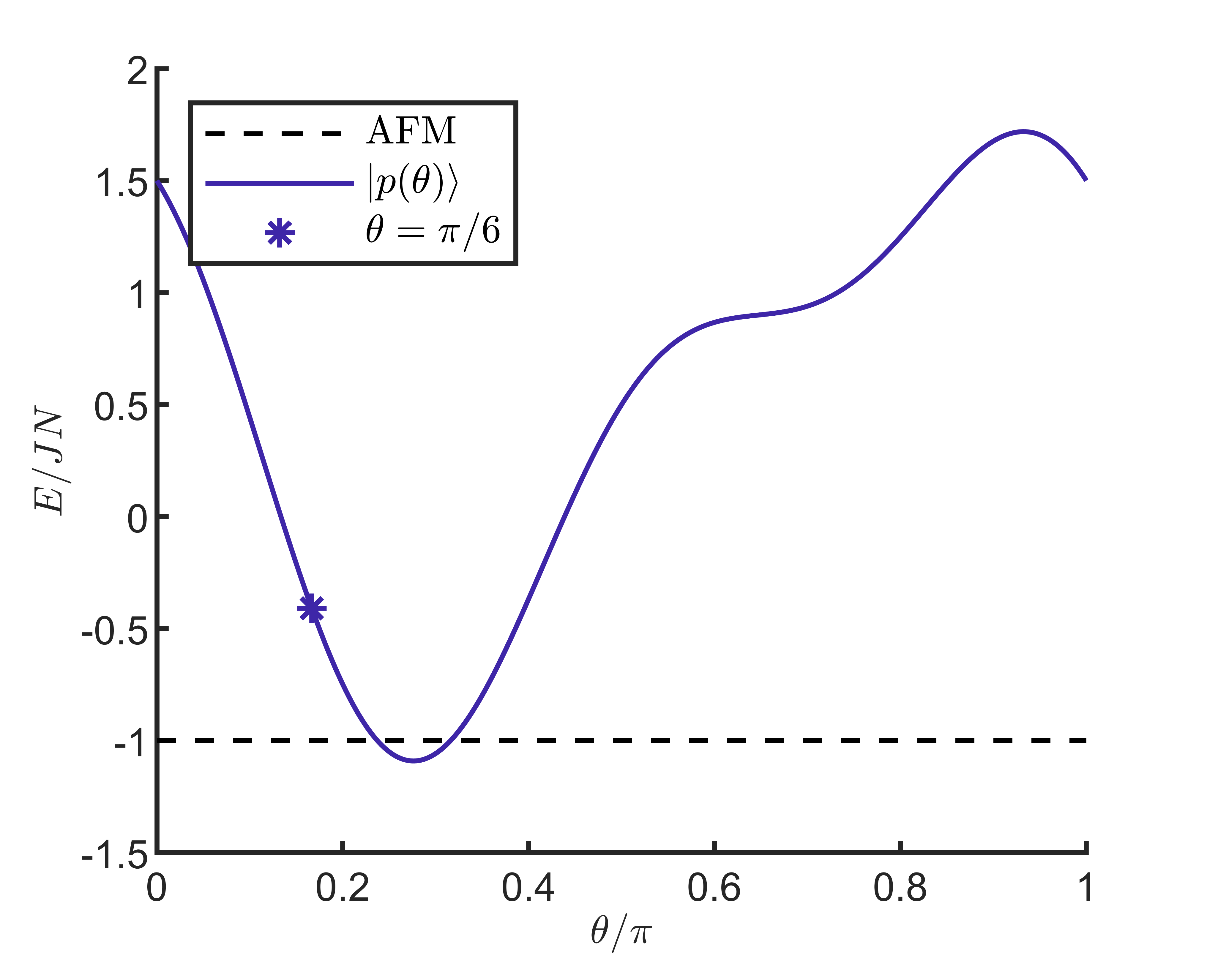
Figure 6: $E/JN$ dependence on the parameter $\theta$. We have marked the $\theta=\pi/6$ value used in the work. The AFM state has $E/JN=-1$ in the thermodynamic limit.

Appendix E MPS investigation

We have limited the numerics in Section III to only exact calculations for small systems. One could expect that matrix product state (MPS) methods [26] would allow us to reach larger system sizes. However, this proves to be a very challenging task. In this appendix, we provide details about the drawbacks of such MPS calculations for this particular model and illustrate why it is hard to go beyond the system sizes accessible with the exact methods.

Firstly, we investigate the ground state of $\mathcal{H}$ using DMRG. In Fig. 7, we show that we approach the ground state slowly in the number of sweeps. As shown in the figure, which illustrates the ground state search corresponding already for a small system size $N=16$ (which can be solved with exact diagonalization), even after 1000 sweeps, the error in the energy is considerably large (note that the exact value is zero).

Secondly, we look at the entanglement entropy of the filtered states and how it depends on the system size $N$ and $\delta^{-1}$ to understand the fundamental limitations in their approximability as MPS. Fig. 8 shows the dependence of the entropy of half chain with $\delta^{-1}$ for various system sizes, obtained from our exact calculations. The results indicate a tendency to a linear increase with $N$ for sufficiently small $\delta$, consistent with a volume law. We thus conclude that the MPS techniques will not be able to efficiently capture the ground state, respectively, the adiabatic evolution of the parent Hamiltonian $\mathcal{H}$. This behavior is expected since we are trying to approximate an energy eigenstate at the center of the spectrum, which follows the volume law of entanglement. The inability to express these states as MPS further solidifies the need for a quantum algorithm that is capable of preparing such states and investigating their properties.

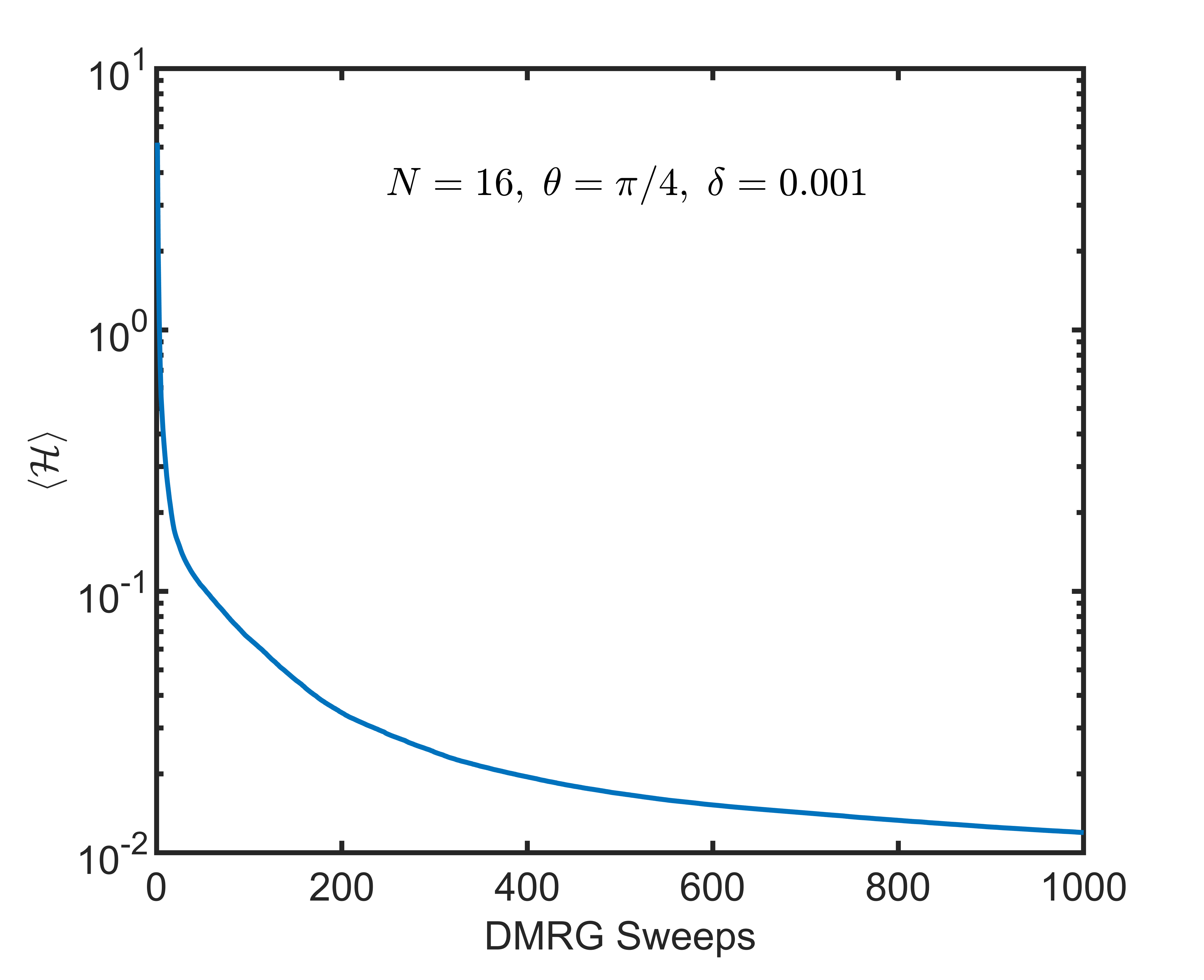
Figure 7: The figure shows the decay of the parent Hamiltonian $\mathcal{H}$ energy with the number of DMRG sweeps. The convergence to the true value of $\expectationvalue{\mathcal{H}}=0$ happens slowly.

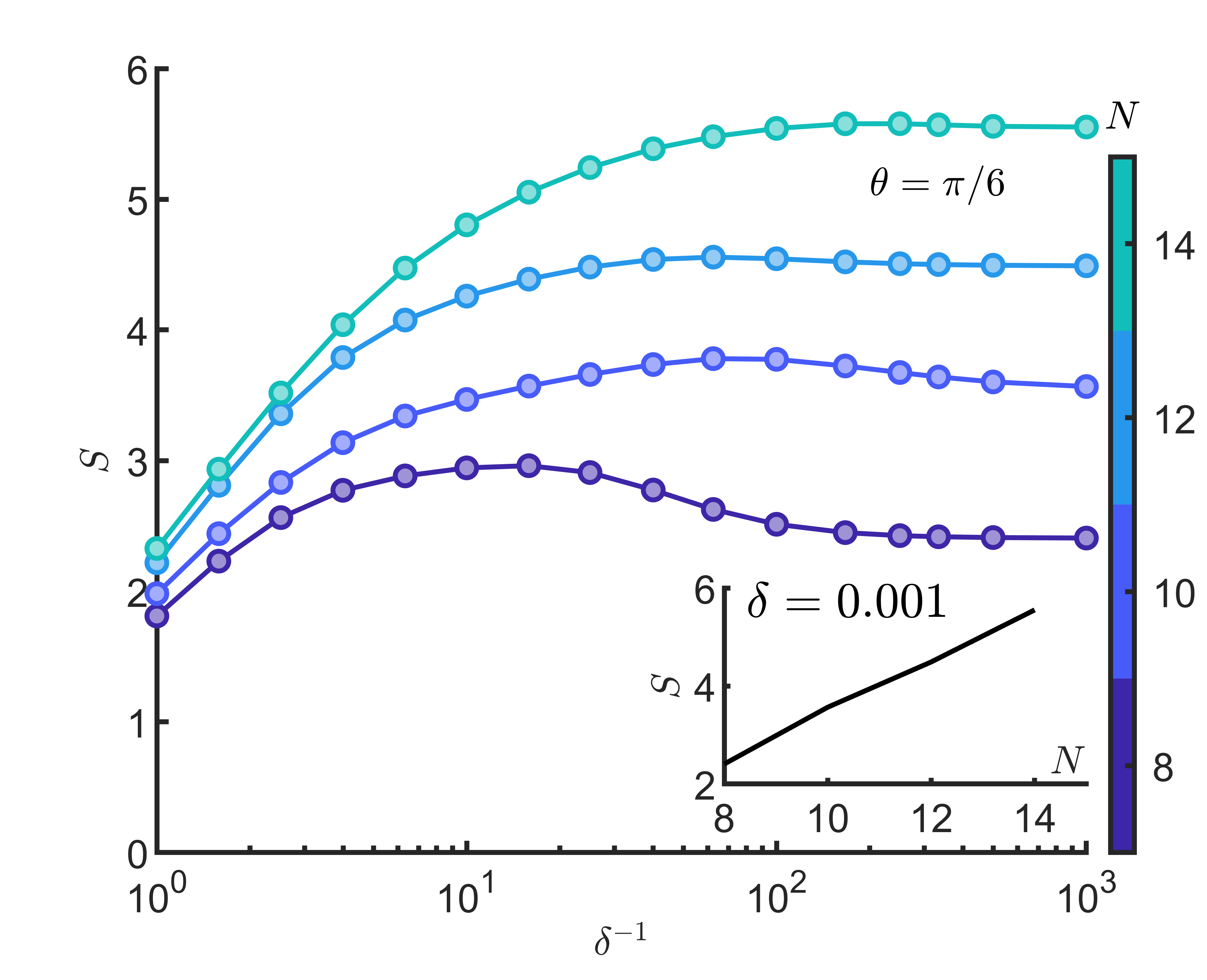
Figure 8: The figure shows the dependence of the bipartite entanglement entropy with $\delta^{-1}$ and for various system sizes $N$. We observe that for a given $\delta^{-1}$, the entanglement grows linearly with $N$.