Metropolis-adjusted interacting particle sampling

Abstract

In recent years, various interacting particle samplers have been developed to sample from complex target distributions, such as those found in Bayesian inverse problems. These samplers are motivated by the mean-field limit perspective and implemented as ensembles of particles that move in the product state space according to coupled stochastic differential equations. The ensemble approximation and numerical time stepping used to simulate these systems can introduce bias and affect the invariance of the particle system with respect to the target distribution. To correct for this, we investigate the use of a Metropolization step, similar to the Metropolis-adjusted Langevin algorithm. We examine Metropolization of either the whole ensemble or smaller subsets of the ensemble, and prove basic convergence of the resulting ensemble Markov chain to the target distribution. Our numerical results demonstrate the benefits of this correction in numerical examples for popular interacting particle samplers such as ALDI, CBS, and stochastic SVGD.

Keywords: Metropolis-Hastings, interacting particle systems, Bayesian inference

1 Introduction

Generating samples or computing expectations with respect to a given target distribution $\pi$ in $\mathbb{R}^{d}$ is a ubiquituous task in applied mathematics, computational physics, statistics, and data science. Applications are broad and include for example Bayesian inference, generative modeling, and hypothesis testing and model fitting.

Various methods tackling this problem have been proposed and analyzed in the literature. A classical and nowadays standard method is Markov-Chain Monte Carlo (MCMC) [2] and, in particular, the popular Metropolis-Hastings (MH) algorithm [27, 16]. Recently, novel approaches that couple the target distribution with a reference distribution $\pi_{0}$ through a deterministic “transport map” have emerged, such as polynomial transports [26, 19], tensor-train transports [8], normalizing flows [34], and neural ODEs [4]. The resulting sampling methods aim to transform initial iid samples following the reference distribution to samples (approximately) following the target distribution by applying the transport map samplewise.

Another way to achieve such a transformation of an initial ensemble of particles or samples following $\pi_{0}$ is by applying suitable stochastic dynamics to the ensemble which for time $t\to\infty$ yield particles approximately distributed according to the target $\pi$. The resulting ensemble dynamics are often interacting, i.e., the drift or diffusion term for each particle depends on the whole ensemble. Such stochastic interacting particle systems emerge from various ideas and approaches: (i) as ensemble approximations of $\pi$-invariant stochastic differential equations of Langevin or McKean-Vlasov type [12, 13, 15], (ii) by adapting methods from particle swarm optimization to construct samplers [3], or (iii) from gradient flows to minimize some objective quantifying the difference between the target $\pi$ and a current approximation $\pi_{t}$ [24, 29, 11]. For each of these approaches we consider a particular example in this work: (i) an affine invariant interacting Langevin sampler (ALDI) [12, 13], (ii) a consensus-based sampler (CBS) [3], and (iii) a stochastic version of Stein variational gradient descent (SVGD) [11].

In practice, simulating the resulting stochastic dynamical system requires a time discretization and a suitable numerical integration scheme. For example, approximating the Langevin dynamics via the Euler-Maruyama scheme leads to the so-called unadjusted Langevin algorithm (ULA) [39]. For ULA it can be shown that the time-stepping scheme causes a bias, so that the limiting distribution has an error of the size of the time discretization step, see e.g. [42, Theorem 2]. The Metropolis-adjusted Langevin algorithm (MALA) circumvents this problem by introducing an MH acceptance/rejection-step after each Langevin update [1, 39].

In this paper, we propose a similar approach for recent interacting particle systems with $M\in\mathbb{N}$ particles. That is, we view the time-discrete interactive update of the particles as a proposal within an MH scheme. This results in a Markov chain in the $M$-fold product space, $\mathbb{R}^{d}\times\cdots\times\mathbb{R}^{d}\simeq\mathbb{R}^{Md}$, that corrects for the bias introduced by the time-discretization of the ensemble dynamics. Additionally, it offers a natural approach to parallelize Markov chain Monte Carlo sampling, and potentially leads to improved proposals due the whole ensemble’s information being used.

The concept of ensemble MCMC was first introduced in [5, 14], where particles, referred to as “walkers”, are updated individually using so-called walk or stretch moves that involve only two of the $M$ particles. Following [14] further ensemble MCMC algorithms have been proposed in recent years [7, 10, 22]. In these works the ensemble is used to estimate the target covariance empirically. The ensemble covariance is then applied as a preconditioner or covariance for proposing new states based on a Gauss-Newton update or the (generalized) preconditioned Crank-Nicolson proposal [6, 40], respectively. Similar to [14], the authors of [7, 10, 22] use a sequential particle-wise update and, hence, Metropolization.

Outline

The remainder of this paper is organized as follows: In this section, we explain interacting particle systems and present our main ideas, describe our contributions, and introduce notation. In Section 2, we review the basic methodology of the Metropolis-Hastings algorithm, including the specific instance known as “MALA”, and also discuss classic results related to its convergence. In Section 3, we present three general strategies of Metropolizing interacting particle systems—ensemble-wise, particle-wise and block-wise — and provide convergence results for each of them. Section 4 discusses common examples of interacting particle systems that are based on various underlying stochastic dynamics, and we explain how they align with our Metropolization schemes. Finally, in Section 5 we report on numerical results for all presented interacting particle methods.

Notation and conventions

Throughout we consider an underlying probability space $(\Omega,\mathcal{F},\mathbb{P})$, $\mathbb{R}^{d}$ to be equipped with the Borel $\sigma$-algebra $\mathcal{B}(\mathbb{R}^{d})$, and we assume the target probability distribution $\pi$ on $\mathbb{R}^{d}$ to be absolutely continuous with respect to Lebesgue measure. By abuse of notation, we use the same symbols to denote the Lebesgue densities and the corresponding distributions they represent. Moreover, we denote by $\mathcal{P}(\mathbb{R}^{d})$ the set of probability densities on $\mathbb{R}^{d}$. As usual, ${\rm N}(\mu,\Sigma)$ stands for a normal distribution with mean $\mu\in\mathbb{R}^{d}$ and covariance $\Sigma\in\mathcal{B}(\mathbb{R}^{d})$, and ${\rm U}([0,1])$ denotes a uniform distribution on $[0,1]$.

For a measure $\mu$ on $\mathbb{R}^{d}$ we denote by $L_{\mu}^{1}(\mathbb{R})$ the Lebesgue space of $\mu$-integrable functions $F:\mathbb{R}^{d}\to\mathbb{R}$. Similarly $L_{\mu}^{2}(\mathbb{R})$ stands for the square integrable functions w.r.t. the measure $\mu$. For $F\in L_{\mu}^{1}(\mathbb{R})$ we write $\mathbb{E}_{\mu}[F]:=\int_{\mathbb{R}^{d}}F(x)\mu({\rm d}x)$ and additionally $\mathbb{V}_{\mu}[F]:=\mathbb{E}_{\mu}[(F-\mathbb{E}_{\mu}[F])^{2}]$ in case $F\in L_{\mu}^{2}(\mathbb{R})$.

We write $\mathcal{C}(\mathbb{R}^{d})\subset\mathbb{R}^{d\times d}$ for the set of symmetric positive semidefinite matrices of size $d\times d$. The set of all symmetric positive definite matrices is denoted by $\mathcal{C}^{+}(\mathbb{R}^{d})$ and we write $\sqrt{C}$ for the square root of $C\in\mathcal{C}^{+}(\mathbb{R}^{d})$. The $n$-dimensional identity matrix is denoted by ${\rm Id}_{n}\in\mathbb{R}^{n\times n}$.

We use boldface notation $\mathbf{x}$ to denote vectors in $\mathbb{R}^{Md}$. They are always interpreted as an ensemble of $M$ vectors in $\mathbb{R}^{d}$ which in turn are denoted by $x^{(1)},\dots,x^{(M)}$. The ensemble excluding the $i$th particle will be denoted by $\mathbf{x}^{-(i)}$. More precisely

$$\mathbf{x}:=\begin{pmatrix}x^{(1)}\\ \vdots\\ x^{(M)}\end{pmatrix}\in\mathbb{R}^{Md}\qquad\text{and}\qquad\mathbf{x}^{-(i)}:=\begin{pmatrix}x^{(1)}\\ \vdots\\ x^{(i-1)}\\ x^{(i+1)}\\ \vdots\\ x^{(M)}\end{pmatrix}\in\mathbb{R}^{M(d-1)}.$$ (1)

For random variables we use upper case notation, for example $\boldsymbol{X}=((X^{(1)})^{\top},\dots,(X^{(M)})^{\top})^{\top}$. The notation $\boldsymbol{X}=\mathbf{x}$ signifies that a draw of this random variable yielded the value $\mathbf{x}$ and we use $X^{(i)}\in\mathbb{R}^{d}$ or $\boldsymbol{X}\in\mathbb{R}^{Md}$ as shorthand notation for $X^{(i)}$ being an $\mathbb{R}^{d}$-valued and $\boldsymbol{X}$ being an $\mathbb{R}^{Md}$-valued random variable, respectively.

1.1 Interacting particle systems

The starting point of our method are dynamical systems that transform a single particle $X_{0}\sim\pi_{0}$ at time $t=0$ into a particle following the target distribution $\pi$ as $t\to\infty$. The dynamics of the particle are described by a stochastic differential equation (SDE) of McKean-Vlasov type [30]:

$${\rm d}X_{t}=\phi(X_{t},\pi_{t}){\rm d}t+\sqrt{\sigma(X_{t},\pi_{t})}{\rm d}B_{t},$$ (2)

where $\pi_{t}:\mathbb{R}^{d}\to[0,\infty)$ is the probability density of $X_{t}\in\mathbb{R}^{d}$ at time $t$, $B_{t}\in\mathbb{R}^{d}$ is a (standard) Brownian motion, $\phi:\mathbb{R}^{d}\times\mathcal{P}(\mathbb{R}^{d})\to\mathbb{R}^{d}$ is referred to as the drift, and $\sigma:\mathbb{R}^{d}\times\mathcal{P}(\mathbb{R}^{d})\to\mathcal{C}(\mathbb{R}^{d})$ is the diffusion. Moreover, we assume existence of a unique strong solution $X_{t}$ of (2) throughout the paper.

Example 1.1 (Langevin dynamics).

One classical example of (2) is

$${\rm d}X_{t}=C\nabla\log\pi(X_{t}){\rm d}t+\sqrt{2C}{\rm d}B_{t}$$ (3)

for a fixed covariance matrix $C\in\mathcal{C}^{+}(\mathbb{R}^{d})$. The density $\pi_{t}$ of $X_{t}$ satisfies the corresponding Fokker-Planck equation

$$\partial_{t}\pi_{t}=\nabla\cdot(\pi_{t}C\nabla\log(\pi))+\operatorname{Tr}(C\nabla^{2}\pi_{t}),$$

which describes the gradient flow in the space of probability measures w.r.t. the Wasserstein metric [20]. Under suitable assumptions ($\pi$ satisfies a Poincaré inequality) one can show exponential convergence of $\pi_{t}$ to $\pi$ as $t\to\infty$, e.g., [25].

Note that the drift and diffusion in (3) are independent of $\pi_{t}$. This is in contrast to the closely related “Kalman-Wasserstein dynamics” [12]: replacing $C$ with

$$C(\pi_{t}):=\int_{\mathbb{R}^{d}}(x-m(\pi_{t}))(x-m(\pi_{t}))^{\top}\pi_{t}(x)\,\mathrm{d}x\in\mathbb{R}^{d\times d},\qquad m(\pi_{t}):=\int_{\mathbb{R}^{d}}x\pi_{t}(x)\,\mathrm{d}x\in\mathbb{R}^{d}$$ (4a)

yields a McKean-Vlasov Langevin dynamic of the form (2) with

$$\phi(x,\rho)=C(\rho)\nabla\log\pi(x),\qquad\sigma(x,\rho)=2C(\rho),$$ (4b)

for $x\in\mathbb{R}^{d}$ and $\rho\in\mathcal{P}(\mathbb{R}^{d})$.

For strongly log-concave target measures $\pi$ and under the additional assumption that $C(\pi_{t})$ does not degenerate, the resulting Markov process $(X_{t})_{t\geq 0}$ is ergodic with unique invariant distribution $\pi$ and it holds exponential convergence of $\pi_{t}$ to $\pi$ in the Kullback-Leibler divergence as $t\to\infty$ [12, Proposition 2]. Potential advantages of replacing $C$ by $C(\pi_{t})$ are (i) faster convergence of $\pi_{t}\to\pi$ due to the preconditioning and (ii) affine-invariance of the resulting dynamics, see [13, 22].

Ensemble discretization

Solving (2) by numerical methods requires to discretize. In terms of the distribution $\pi_{t}$, this is achieved by replacing $\pi_{t}$ with the empirical distribution of an ensemble of $M\in\mathbb{N}$ particles $X^{(i)}_{t}\in\mathbb{R}^{d}$, $i=1,\dots,M$, initialized iid as $X_{0}^{(i)}\sim\pi_{0}$, $i=1,\dots,M$, at time $t=0$. The particles are collected into a vector $\boldsymbol{X}_{t}\in\mathbb{R}^{Md}$ representing the state of the whole ensemble (cp. (1)). Equation (2) then formally becomes a coupled system of SDEs

$${\rm d}\boldsymbol{X}_{t}=\boldsymbol{\Phi}(\boldsymbol{X}_{t})\,{\rm d}t+\sqrt{\boldsymbol{\Sigma}(\boldsymbol{X}_{t})}\,{\rm d}\boldsymbol{B}_{t},$$ (5)

for some suitable drift, diffusion, and standard Brownian motion

$$\boldsymbol{\Phi}:\mathbb{R}^{Md}\to\mathbb{R}^{Md},\qquad\boldsymbol{\Sigma}:\mathbb{R}^{Md}\to\mathcal{C}(\mathbb{R}^{Md}),\qquad\boldsymbol{B}_{t}\in\mathbb{R}^{Md}.$$

Again, we assume well-definedness of the solution $\boldsymbol{X}_{t}$ of (5) throughout.

Remark 1.2.

Some papers proceed by first proposing a discrete system of the type (5), and then studying the mean field limit (2) obtained as $M\to\infty$.

Example 1.3 (Interacting Langevin Dynamics).

We continue the example of McKean-Vlasov Langevin dynamics from Example 1.1

$${\rm d}X_{t}=C(\pi_{t})\nabla\log\pi(X_{t}){\rm d}t+\sqrt{2C(\pi_{t})}{\rm d}B_{t}.$$ (6)

The computation of $C(\pi_{t})$ in (4a) requires to approximate an integral w.r.t. $\pi_{t}$. Using Monte Carlo integration based on an ensemble of $M$ particles following these dynamics we obtain the ensemble version [12] of the mean-field dynamics (6)

$${\rm d}X_{t}^{(i)}=C(\boldsymbol{X}_{t})\nabla_{x}\log\pi(X_{t}^{(i)})+\sqrt{2C(\boldsymbol{X}_{t})}{\rm d}B_{t}^{(i)}\qquad i\in\{1,\dots,M\},$$ (7)

where

$$C(\boldsymbol{X}_{t}):=\frac{1}{M}\sum_{i=1}^{M}\left(X_{t}^{(i)}-m(\boldsymbol{X}_{t})\right)\left(X_{t}^{(i)}-m(\boldsymbol{X}_{t})\right)^{\top}\in\mathcal{C}(\mathbb{R}^{d}),\qquad m(\boldsymbol{X}_{t})=\frac{1}{M}\sum_{i=1}^{M}X_{t}^{(i)}\in\mathbb{R}^{d}$$ (8)

denote the empirical covariance and mean of the ensemble $\boldsymbol{X}_{t}$. Note that the system of SDEs (7) is completely coupled since individual particles interact via $C(\boldsymbol{X}_{t})$.

It can be shown that the invariant distribution of the particles in (7) in general may have a bias, i.e. does not equal $\pi$. To address this issue, the authors in [28] propose the following modification:

$${\rm d}X_{t}^{(i)}=C(\boldsymbol{X}_{t})\nabla\log\pi(X_{t}^{(i)})+\frac{d+1}{M}(X_{t}^{(i)}-m(\boldsymbol{X}_{t}))+\sqrt{2C(\boldsymbol{X}_{t})}{\rm d}B_{t}^{(i)}\qquad i\in\{1,\dots,M\}.$$ (9)

Time discretization

Besides discretizing the distribution, a numerical time-stepping scheme to approximately simulate (5) is required. For a fixed time step size $h>0$, let $\boldsymbol{\zeta}_{k}\sim\mathrm{N}(0,{\rm I}_{Md})$, $k\in\mathbb{N}$, i.e. $\boldsymbol{\zeta}_{k}\in\mathbb{R}^{Md}$ is normally distributed with mean $0$ and covariance matrix given by the $Md$-dimensional identity matrix ${\rm I}_{Md}$. Then the Euler-Maruyama discretization of (5) reads

$$\boldsymbol{X}_{k+1}=\boldsymbol{X}_{k}+h\boldsymbol{\Phi}(\boldsymbol{X}_{k})+\sqrt{h\boldsymbol{\Sigma}(\boldsymbol{X}_{k})}\boldsymbol{\zeta}_{k+1}$$ (10)

with $\boldsymbol{X}_{k}=(X_{k}^{(1)},\dots,X_{k}^{(M)})\in\mathbb{R}^{Md}$ and initialized as $X_{0}^{(i)}\sim\pi_{0}$ iid for $i=1,\dots,M$.

Example 1.4 (Unadjusted Langevin algorithm).

The Langevin dynamics (3) do not require an ensemble approximation. However, we may consider $M$ particles $X_{t}^{(i)}$, $i=1,\ldots,M$, each individually following (3) without interaction. This can be viewed as (non-interacting) ensemble dynamics of the form (5). The corresponding time-discretized system is

$$X_{k+1}^{(i)}=X_{k}^{(i)}+hC\nabla\log\pi(X_{k}^{(i)})+\sqrt{2hC}\zeta_{k+1}^{(i)},\qquad i\in\{1,\dots,M\},$$ (11)

with $\zeta_{k+1}^{(i)}\sim\mathrm{N}(0,{\mathrm{Id}}_{d})$ iid. For $C={\rm Id}_{d}$, this is known as the (parallel) ULA [15, 39].

Example 1.5 (Unadjusted interacting Langevin dynamics).

For the interacting Langevin dynamics (9), we obtain the time-discrete interacting particle system

$$X_{k+1}^{(i)}=X_{k}^{(i)}+hC(\boldsymbol{X}_{k})\nabla\log\pi(X_{k}^{(i)})+h\frac{d+1}{M}(X_{k}^{(i)}-m(\boldsymbol{X}_{k}))+\sqrt{2hC(\boldsymbol{X}_{k})}\zeta_{k+1}^{(i)}\quad i\in\{1,\dots,M\},$$ (12)

with $\zeta_{k+1}^{(i)}\sim\mathrm{N}(0,{\mathrm{Id}}_{d})$ and $C(\boldsymbol{X}_{k})$ as in (8).

It is well-known that the introduction of the time discretization may lead to a bias, i.e. in general it does not hold that $X_{k}^{(i)}$ converges in distribution to $\pi$ as $k\to\infty$. This applies for example to ULA [42].

1.2 Main idea and contributions

Julian Besag [1] suggested in 1994 to correct the unadjusted Langevin algorithm with a Metropolization to obtain a $\pi$-invariant one-particle Markov chain $(X_{k})_{k\in\mathbb{N}}$, which lead to MALA. We adopt this idea to correct for the bias in general time-discrete interacting particle systems (10). To this end, we view (10) as the proposal mechanism for an ensemble Markov chain $(\boldsymbol{X}_{k})_{k\in\mathbb{N}}$ in the product state space $\mathbb{R}^{Md}$. We propose to apply Metropolization in three ways: (i) ensemble-wise, i.e., accept or reject the whole ensemble of all proposed particles, (ii) particle-wise, i.e., accept or reject each proposed particle individually in a sequential manner, and (iii) block-wise, i.e., accept or reject each block of particles individually in a sequential manner. Here a block is understood as a fixed subset of particles and identified with $\mathbf{b}\subset\{1,\ldots,M\}$. Methods (i) and (ii) can be seen as a special case of (iii) with either just one batch representing the whole ensemble, or batches consisting of only one particle. Due to their different algorithmic behaviour and to present clearly the underlying train of thought we will discuss the three versions separately. A high-level version of the novel block-wise Metropolization is summarized in Algorithm 1.

Moreover, we discuss also a simultaneous version of particle-wise Metropolization in this work. Such a method is computationally appealing, as it enables particle-wise parallelization. However, it turns out that this strategy can, in general, yield a biased algorithm, i.e., the ensemble Markov chain does not have the correct invariant measure. We provide specific examples for the bias of simultaneous particle-wise Metropolization in Appendix A.

1:fix a partition $\bigcup_{j=1}^{L}\mathbf{b}_{j}=\{1,\dots,M\}$

2:draw $\mathbf{x}_{0}\in\mathbb{R}^{Md}$ according to $\otimes_{i=1}^{M}\pi_{0}$ and set initial ensemble state $\boldsymbol{X}_{0}=\mathbf{x}_{0}$

3:for $k=0,\dots,N$ do

4:     given $\boldsymbol{X}_{k}=\mathbf{x}_{k}$ initialize $\mathbf{x}=(x^{(1)},\ldots,x^{(M)})$ by $\mathbf{x}=\mathbf{x}_{k}$

5:     for $j=1,\dots,L$ do

6:         draw block proposal $(y^{(i)})_{i\in\mathbf{b}_{j}}\in\mathbb{R}^{|\mathbf{b}_{j}|d}$ according particle proposals such as (11) or (12) based on current ensemble $\mathbf{x}$

7:         update $(x^{(i)})_{i\in\mathbf{b}_{j}}=(y^{(i)})_{i\in\mathbf{b}_{j}}$ only with block acceptance probability

8:     end for

9:     set $\boldsymbol{X}_{k+1}=\mathbf{x}$

10:end for

11:return ensemble chain $(\boldsymbol{X}_{k})_{k=0}^{N+1}$

Algorithm 1 Block-wise Metropolization

We emphasize the following potential advantages of combining the Metropolis-Hastings mechanism with interacting particle systems:

• From an interacting particle sampling perspective we correct for the immanent bias of the particle dynamics due to numerical time-stepping schemes and finite ensemble approximations of $\phi(\cdot,\pi_{t})$ and $\sigma(\cdot,\pi_{t})$ in (2). In particular, this allows in principle to take large time steps $h$ in (10) without provoking an instability of the time-discrete dynamical system.

• From an MCMC sampling perspective the interacting particle dynamics provide in each iteration not just one new state $x_{k}\in\mathbb{R}^{d}$ but $M$ new states which can be computed in parallel which yields a computational advantage. Moreover, in comparison to simply performing, e.g., parallel MALA, the interaction of the particles may yield more efficient proposal kernels due to estimating, e.g., the target covariance empirically by the ensemble, and, thus, lead to more efficient MCMC sampling. In particular, we obtain affine-invariant MCMC methods if the underlying interacting particle dynamics are affine-invariant themselves such as those proposed in [12, 13, 3].

Contributions

We summarize the main contributions of this paper:

1. We propose a new MCMC method by combining a Metropolization step with interacting particle dynamics in the $M$-fold product state space.

2. We discuss several variants of this method for differing sizes of the blocks which are Metropolized. Basic convergence results as well as numerical indications suggesting that suitable choices of block sizes lead to more efficient sampling algorithms are presented.

3. We give several concrete examples based on different particle dynamics, including the recently introduced stochastic SVGD [29, 11], ALDI [12, 13], and CBS [3].

4. We present numerical experiments to compare the different variants of our algorithm, demonstrating in particular improved robustness and higher efficiency due to interaction and (block-wise) Metropolization.

5. In the appendix, we provide counterexamples to show that a simultaneous particle-wise Metropolization strategy does in general not yield an unbiased algorithm.

2 Preliminaries on Markov chain Monte Carlo

We recall the basic terminology and ideas of MCMC sampling required in the following.

Throughout let $\pi$ be a given absolutely continuous (target) probability distribution on $\mathbb{R}^{d}$ with the Lebesgue density also denoted by $\pi:\mathbb{R}^{d}\to[0,\infty)$. To approximately sample from $\pi$, we construct a Markov chain $(X_{k})_{k\in\mathbb{N}}\subseteq\mathbb{R}^{d}$ that converges to $\pi$ in distribution as $k\to\infty$. We denote the associated transition kernel by $P:\mathbb{R}^{d}\times\mathcal{B}(\mathbb{R}^{d})\to[0,1]$, i.e., the chain is characterized by $X_{k}=x$ implying $X_{k+1}\sim P(x,\cdot)$. For a measure $\mu$ on $\mathbb{R}^{d}$ we use the usual notation $\mu P$ for the measure

$$\mu P(A):=\int_{\mathbb{R}^{d}}P(z,A)\mu(dz)\qquad\forall A\in\mathcal{B}(\mathbb{R}^{d})$$

and inductively $\mu P^{k}:=(\mu P^{k-1})P$ for all $k\geq 2$. Note that if $X_{0}\sim\pi_{0}$ for some initial distribution $\pi_{0}$ then $X_{k}\sim\pi_{0}P^{k}$.

We say that

• $\pi$ is an invariant measure of $P$ iff

  $$\pi=\pi P,$$

  in which case we call $P$ and $(X_{k})_{k\in\mathbb{N}}$ $\pi$-invariant,

• the Markov chain is $\pi$-reversible iff it satisfies the detailed balance condition

  $$\int_{A}P(x,B)\pi({\rm d}x)=\int_{B}P(z,A)\pi({\rm d}z)\qquad\forall A,B\in\mathcal{B}(\mathbb{R}^{d}),$$ (13)

• the Markov chain is ergodic iff it holds

  $$\lim_{k\to\infty}d_{\rm TV}(\pi_{0}P^{k},\pi)=0,$$ (14)

  where $\pi_{0}$ is the initial distribution and $d_{\rm TV}$ stands for the total variation distance,

• the Markov chain satisfies a strong law of large numbers iff

  $$S_{N}(F):=\frac{1}{N}\sum_{k=1}^{N}F(X_{k})\xrightarrow[N\to\infty]{\text{a.\ s.}}\ \mathbb{E}_{\pi}[F]\qquad\forall F\in L^{1}_{\pi}(\mathbb{R}),$$ (15)

• the Markov chain satisfies a central limit theorem for $F\in L_{\pi}^{2}(\mathbb{R})$ iff there exists $\sigma^{2}_{F}\in[0,\infty)$ such that

  $$\sqrt{N}\left(S_{N}(F)-\mathbb{E}_{\pi}[F]\right)\ \xrightarrow[N\to\infty]{\mathcal{L}}\ \mathrm{N}\left(0,\sigma_{F}^{2}\right).$$ (16)

Due to $X_{k}\sim\pi_{0}P^{k}$, the Markov chain $(X_{k})_{k\in\mathbb{N}}$ can be interpreted as the realization of a fixed point iteration under the mapping $P$. Hence $\pi$ being an invariant measure of $P$ is a necessary condition to obtain ergodicity. Additionally, let us mention that $\pi$-reversibility is sufficient to ensure $\pi$-invariance.

For Markov chains with $\pi$-reversible transition kernel $P$ the asymptotic variance $\sigma^{2}_{F}$ of $S_{N}(F)$ in (16) can, in case of existence, be expressed by

$$\sigma_{F}^{2}=\mathbb{V}_{\pi}[F]\left[1+2\sum_{k=1}^{\infty}\mathrm{Corr}(F(\tilde{X}_{0}),F(\tilde{X}_{0+k})\right],$$ (17)

where $(\tilde{X}_{k})_{k\in\mathbb{N}}$ denotes the $\pi$-reversible Markov chain with transition kernel $P$ starting in stationarity $\tilde{X}_{0}\sim\pi$. While a strong law of large numbers holds under mild conditions, the central limit theorem is more nuanced. We refer to [37, Section 5] for more details.

2.1 Metropolis-Hastings algorithm

The key question is how to obtain transition kernels that ensure ergodicity and a strong law of large numbers. The MH algorithm [27, 16] is a standard method achieving this under rather mild assumptions.

The algorithm is based on a proposal kernel $Q\colon\mathbb{R}^{d}\times\mathcal{B}(\mathbb{R}^{d})\to[0,1]$, that assigns a probability measure $Q(x,\cdot)$ on $\mathbb{R}^{d}$ to every $x\in\mathbb{R}^{d}$, in combination with an acceptance-rejection step. Throughout, we assume that $Q(x,\cdot)$ possesses a Lebesgue density for each $x\in\mathbb{R}^{d}$, i.e. there exists $q:\mathbb{R}^{d}\times\mathbb{R}^{d}\to[0,\infty)$ such that

$$Q(x,A)=\int_{A}q(x,y)\ {\rm d}y\qquad\forall A\in\mathcal{B}(\mathbb{R}^{d}).$$

In the $k$th step, if $X_{k}=x_{k}$ and $y_{k+1}$ is a proposed value drawn from $Q(x_{k},\cdot)$, then $X_{k+1}$ is set to $y_{k+1}$ with probability $\alpha(x_{k},y_{k+1})$ defined as follows:

$$\alpha(x_{k},y_{k+1}):=\begin{cases}\min\left(1,\frac{\pi(y_{k+1})q(y_{k+1},x_{k})}{\pi(x_{k})q(x_{k},y_{k+1})}\right)&\text{if }\pi(x_{k})q(x_{k},y_{k+1})>0\\ 1&\text{otherwise}.\end{cases}$$ (18)

If $X_{k+1}$ is not set to $y_{k+1}$, it is set to $x_{k}$. The resulting transition kernel is

$$P(x,{\rm d}y)=\alpha(x,y)q(x,y){\rm d}y+r(x)\delta_{x}({\rm d}y),\qquad r(x):=1-\int_{\mathbb{R}^{d}}\alpha(x,y)q(x,y){\rm d}y.$$ (19)

It can easily be checked that $P$ is in fact $\pi$-reversible. We present the full algorithm in Algorithm 2 and refer to [35, Section 7.3] for more details.

1:Input:

• target density $\pi$ on $\mathbb{R}^{d}$

• proposal kernel $Q$ with density $q:\mathbb{R}^{d}\times\mathbb{R}^{d}\to(0,\infty)$

• initial probability distribution $\pi_{0}$ on $\mathbb{R}^{d}$

2:Output: Markov chain $(X_{k})_{k\in\{1,\dots,N\}}$ in state space $\mathbb{R}^{d}$

3:draw $x_{0}\sim\pi_{0}$ and set initial state $X_{0}=x_{0}$

4:for $k=0,\dots,N$ do

5:     given $X_{k}=x_{k}$ draw proposal $y_{k+1}\sim Q(x_{k},\cdot)$

6:     compute acceptance probability $\alpha(x_{k},y_{k+1})$ in (18)

7:     draw $u\sim{\rm U}([0,1])$ and set

$$X_{k+1}=\begin{cases}y_{k+1}&\text{if}\ u\leq\alpha(x_{k},y_{k+1})\\ x_{k}&\text{else}\end{cases}$$

8:end for

Algorithm 2 Metropolis-Hastings

It is left to choose a suitable proposal kernel $Q$. As we recall next, ergodicity is already ensured if $Q(x,\cdot)$ has a positive Lebesgue density $q$, i.e. $q(x,y)>0$ for all $x,y\in\mathbb{R}^{d}$. Nonetheless, in practice the efficiency of the algorithm crucially depends on the choice of $Q$. A standard (albeit crude) proposal satisfying the positivity condition is $Q(x,\cdot)=\mathrm{N}(x,h{\rm Id}_{d})$, $h>0$, also known as Random Walk-MH algorithm.

Theorem 2.1 ([35, Section 6.7.2 and 7.3.2]).

Let $\pi$ be absolutely continuous and let $Q$ possess a positive Lebesgue density $q:\mathbb{R}^{d}\times\mathbb{R}^{d}\to(0,\infty)$, and let $\pi_{0}$ be any initial probability distribution. Then, the Markov chain $(X_{k})_{k\in\mathbb{N}}$ generated by Algorithm 2 with $X_{0}\sim\pi_{0}$

1. is ergodic (14) and satisfies a strong law of large numbers (15),

2. satisfies the central limit theorem (16) for any $F\in L_{\pi}^{2}(\mathbb{R})$ for which $\sigma_{F}^{2}$ in (17) is nonzero and finite.

2.2 Metropolis-adjusted Langevin algorithm

A popular proposal kernel $Q$ is obtained through the Euler-Maruyama discretization

$$X_{k+1}=X_{k}+h\nabla\log\pi(X_{k})+\sqrt{2h}\xi_{k+1},\quad\xi_{k+1}\sim\mathrm{N}(0,{\mathrm{Id}_{d}})$$ (20)

of the Langevin dynamics (3) (with $C={\rm Id}_{d}$) introduced in Example 1.1. Here $h>0$ is a fixed step size, and generating a Markov chain $(X_{k})_{k\in\mathbb{N}}$ through (20) is also known as the unadjusted Langevin algorithm (ULA). While the continuous dynamics (3) has $\pi$ as an invariant distribution, see e.g., [31], it is known that the Markov chain (20) has a bias that scales linearly in $h$ [42, Theorem 2].

Nevertheless, the continuous-time result suggests using (20) as the proposal mechanism, yielding a proposal kernel $Q$ with positive Lebesgue density

$$q(x,y)=\frac{1}{\left(4\pi h\right)^{d/2}}\exp\left(-\frac{1}{4h}\|y-x-h\nabla\log\pi(x)\|^{2}\right).$$

Algorithm 2 with this choice of proposal kernel is known as MALA. According to Theorem 2.1, and contrary to the Markov chain (20), the Metropolised Markov chain generated by Algorithm 2 necessarily does have $\pi$ as its invariant distribution. Moreover, it satisfies ergodicity and a law of large numbers. Furthermore, it is known that for sufficiently large $d$ the best performance in terms of a small asymptotic variance $\sigma_{F}^{2}$ in (16) is obtained for choosing the step size $h$ such that the average acceptance rate $\bar{\alpha}=\int_{\mathbb{R}^{d}}\int_{\mathbb{R}^{d}}\alpha(x,y)q(x,y){\rm d}y\,\pi(x){\rm d}x$ is about $57.4\%$ [36].

3 Metropolis-adjusted interacting particle sampling

We consider an interacting particle system (5) resulting from a finite ensemble approximation of suitable $\pi$-invariant McKean-Vlasov dynamics as in (2), and its time discretization (10) with step size $h>0$, i.e.

$$\boldsymbol{X}_{k+1}=\boldsymbol{X}_{k}+h\boldsymbol{\Phi}(\boldsymbol{X}_{k})+\sqrt{h\boldsymbol{\Sigma}(\boldsymbol{X}_{k})}\boldsymbol{\zeta}_{k+1}.$$ (21)

For many relevant particle methods, there exist

$$\Phi:\mathbb{R}^{d}\times\mathbb{R}^{(M-1)d}\to\mathbb{R}^{d},\qquad\Sigma:\mathbb{R}^{d}\times\mathbb{R}^{(M-1)d}\to\mathcal{C}(\mathbb{R}^{d})$$

such that the drift $\boldsymbol{\Phi}:\mathbb{R}^{Md}\to\mathbb{R}^{d}$ and diffusion $\boldsymbol{\Sigma}:\mathbb{R}^{Md}\to\mathbb{R}^{Md\times Md}$ can be written as

$$\boldsymbol{\Phi}(\boldsymbol{X})=\begin{pmatrix}\Phi(X^{(1)},\boldsymbol{X}^{-(1)})\\ \vdots\\ \Phi(X^{(M)},\boldsymbol{X}^{-(M)})\end{pmatrix},\qquad\boldsymbol{\Sigma}(\boldsymbol{X})=\begin{pmatrix}\Sigma(X^{(1)},\boldsymbol{X}^{-(1)})&&\\ &\ddots&\\ &&\Sigma(X^{(M)},\boldsymbol{X}^{-(M)})\end{pmatrix},$$ (22)

where $\boldsymbol{X}\in\mathbb{R}^{Md}$ denotes again the ensemble of particles $X^{(1)},\dots,X^{(M)}\subseteq\mathbb{R}^{d}$ and we use the notation introduced in (1). In this case the discrete dynamical system (21) takes the form

$$X_{k+1}^{(i)}=X_{k}^{(i)}+h\Phi(X_{k}^{(i)},\boldsymbol{X}_{k}^{(-i)})+\sqrt{h\Sigma(X_{k}^{(i)},\boldsymbol{X}_{k}^{(-i)})}\xi_{k+1}^{(i)}\in\mathbb{R}^{d}\qquad\forall i\in\{1,\dots,M\}$$ (23)

with $\xi_{k}^{(i)}\sim\mathrm{N}(0,{\rm I}_{d})$, iid for all $i\in\{1,\dots,M\}$, $k\in\mathbb{N}$.

In this section we will discuss an ensemble-wise Metropolization for the general dynamics (21) and, in addition, a particle-wise Metropolization for the special case (23) under assumption (22). We emphasize that there are common interacting particle systems, such as SVGD, which do not satisfy (22).

Remark 3.1.

Equation (21) generates an ensemble Markov chain $(\boldsymbol{X}_{k})_{k\in\mathbb{N}}$ in the product state space $\mathbb{R}^{Md}$. We emphasize that the dynamics of each individual particle $(X^{(i)}_{k})_{k\in\mathbb{N}}$, $i=1,\ldots,M$, does not necessarily satisfy the Markov property with respect to the filtration $\mathcal{F}_{t}^{(i)}=\sigma(X_{s}^{(i)},s\leq t)$, since the particle-wise drift and diffusion term may depend on the entire ensemble $\boldsymbol{X}_{k}$.

3.1 Ensemble-wise Metropolization

Our goal in the following is to generate a Markov Chain $(\boldsymbol{X}_{k})_{k\in\mathbb{N}}$ that converges in distribution to the product target measure

$$\boldsymbol{\pi}(\mathbf{x})=\prod_{i=1}^{M}\pi(x^{(i)}).$$

To this end, given the state $\boldsymbol{X}_{k}$, we use (21) to generate the ensemble proposal

$$\boldsymbol{Y}_{k+1}=\boldsymbol{X}_{k}+h\boldsymbol{\Phi}(\boldsymbol{X}_{k})+\sqrt{h\boldsymbol{\Sigma}(\boldsymbol{X}_{k})}\boldsymbol{\zeta}_{k+1}$$ (24)

in the $k$th step of the algorithm. Here as before $\boldsymbol{\zeta}_{k+1}\sim\mathrm{N}(0,{\rm I}_{Md})$, so that the proposal kernel $\mathbf{Q}\colon\mathbb{R}^{Md}\times\mathcal{B}(\mathbb{R}^{Md})\to[0,1]$ on the product space $\mathbb{R}^{Md}$ is given by

$$\mathbf{Q}(\mathbf{x},\cdot)=\mathrm{N}\left(\mathbf{x}+h\boldsymbol{\Phi}(\mathbf{x}),h\boldsymbol{\Sigma}(\mathbf{x})\right)\qquad\forall\mathbf{x}\in\mathbb{R}^{Md}.$$

In order for $\mathbf{Q}(\mathbf{x},\cdot)$ to possess a well-defined Lebesgue density, throughout we assume the following:

Assumption 3.2.

For each $\mathbf{x}\in\mathbb{R}^{Md}$ the matrix $\boldsymbol{\Sigma}(\mathbf{x})\in\mathbb{R}^{Md\times Md}$ in (21) is regular.

The Lebesgue density of $\mathbf{Q}(\mathbf{x},\cdot)$ then reads

$$\mathbf{q}(\mathbf{x},\mathbf{y})=\frac{1}{\det\left(2\pi\,h\,\boldsymbol{\Sigma}(\mathbf{x})\right)^{1/2}}\exp\left(-\frac{1}{2h}\left\|\boldsymbol{\Sigma}(\mathbf{x})^{-1/2}\left(\mathbf{y}-\mathbf{x}-h\boldsymbol{\Phi}(\mathbf{x})\right)\right\|^{2}\right)\qquad\forall\mathbf{x},\mathbf{y}\in\mathbb{R}^{Md},$$ (25)

which is a positive but in general not symmetric function, i.e. $\mathbf{q}(\mathbf{x},\mathbf{y})>0$ for all $\mathbf{x},\mathbf{y}\in\mathbb{R}^{Md}$ but not necessarily $\mathbf{q}(\mathbf{x},\mathbf{y})\neq\mathbf{q}(\mathbf{y},\mathbf{x})$ if $\mathbf{x}\neq\mathbf{y}$. The existence of a density allows to introduce a Metropolization step as follows: The ensemble proposal $\boldsymbol{Y}_{k+1}$ in (24) is accepted with probability

$$\boldsymbol{\alpha}(\boldsymbol{X}_{k},\boldsymbol{Y}_{k+1}):=\begin{cases}\min\left(1,\frac{\boldsymbol{\pi}(\boldsymbol{Y}_{k+1})\,\mathbf{q}(\boldsymbol{Y}_{k+1},\boldsymbol{X}_{k})}{\boldsymbol{\pi}(\boldsymbol{X}_{k})\,\mathbf{q}(\boldsymbol{X}_{k},\boldsymbol{Y}_{k+1})}\right)&\text{if }\boldsymbol{\pi}(\boldsymbol{X}_{k})\mathbf{q}(\boldsymbol{X}_{k},\boldsymbol{Y}_{k+1})>0\\ 1&\text{else,}\end{cases}$$ (26)

in which case we set $\boldsymbol{X}_{k+1}=\boldsymbol{Y}_{k}$. Otherwise $\boldsymbol{X}_{k+1}=\boldsymbol{X}_{k}$. The resulting Metropolis-adjusted interacting particle sampling method is summarised in Algorithm 3.

The corresponding transition kernel $\mathbf{P}\colon\mathbb{R}^{Md}\times\mathcal{B}(\mathbb{R}^{Md})\to[0,1]$ of the ensemble Markov chain $(\boldsymbol{X}_{k})_{k\in\mathbb{N}}$ generated by Algorithm 3 is

$$\mathbf{P}(\mathbf{x},\mathrm{d}\mathbf{y})=\boldsymbol{\alpha}(\mathbf{x},\mathbf{y})\,\mathbf{q}(\mathbf{x},\mathbf{y})\,{\rm d}\mathbf{y}+\mathbf{r}(\mathbf{x})\,\delta_{\mathbf{x}}({\rm d}\mathbf{y}),\qquad\mathbf{r}(\mathbf{x}):=1-\int_{\mathbb{R}^{Md}}\boldsymbol{\alpha}(\mathbf{x},\mathbf{y})\mathbf{q}(\mathbf{x},\mathbf{y})\,{\rm d}\mathbf{y}.$$

Note that the construction allows for general proposal kernels $\mathbf{Q}$ which are dominated by the Lebesgue measure.

1:Input:

• product target density $\boldsymbol{\pi}=\bigotimes_{i=1}^{M}\pi$ on $\mathbb{R}^{Md}$

• proposal kernel $\mathbf{Q}$ with density $\mathbf{q}:\mathbb{R}^{Md}\times\mathbb{R}^{Md}\to(0,\infty)$ in (25)

• initial probability distribution $\pi_{0}$ on $\mathbb{R}^{d}$

2:Output: ensemble Markov chain $(\boldsymbol{X}_{k})_{k\in\{1,\dots,N\}}$ in state space $\mathbb{R}^{Md}$

3:draw $\mathbf{x}_{0}\sim\otimes_{i=1}^{M}\pi_{0}$ and set initial state $\boldsymbol{X}_{0}=\mathbf{x}_{0}$

4:for $k=0,\dots,N$ do

5:     given $\boldsymbol{X}_{k}=\mathbf{x}_{k}$ draw proposal $\mathbf{y}_{k+1}\sim\mathbf{Q}(\mathbf{x}_{k},\cdot)$

6:     compute acceptance probability $\boldsymbol{\alpha}(\mathbf{x}_{k},\mathbf{y}_{k+1})$ in (26)

7:     draw $u\sim{\rm U}([0,1])$ and set

$$\boldsymbol{X}_{k+1}=\begin{cases}\mathbf{y}_{k+1}&\text{if}\ u\leq\boldsymbol{\alpha}(\mathbf{x}_{k},\mathbf{y}_{k+1})\\ \mathbf{x}_{k}&\text{else}\end{cases}$$

8:end for

Algorithm 3 Ensemble-wise Metropolized interactive particle sampling

Algorithm 3 can be interpreted as a Metropolis-Hastings method to sample from the product measure $\boldsymbol{\pi}=\otimes_{i=1}^{M}\pi$ in the product space $\mathbb{R}^{d}\times\cdots\times\mathbb{R}^{d}\simeq\mathbb{R}^{Md}$. Hence the following convergence result is an immediate consequence of Theorem 2.1:

Corollary 3.3.

Let $\pi$ possess a Lebesgue probability density on $\mathbb{R}^{d}$, and let $\pi_{0}$ be any probability distribution on $\mathbb{R}^{d}$. Let $\mathbf{Q}$ possess a positive Lebesgue density $\mathbf{q}:\mathbb{R}^{Md}\times\mathbb{R}^{Md}\to(0,\infty)$, and let $(\boldsymbol{X}_{k})_{k\in\mathbb{N}}$ be generated by Algorithm 3. Then

1. the Markov chain $(\boldsymbol{X}_{k})_{k\in\mathbb{N}}$ is ergodic and satisfies the strong law of large numbers

   $$\mathbf{S}^{M}_{N}(F):=\frac{1}{NM}\sum_{k=1}^{N}\sum_{i=1}^{M}F\left(X^{(i)}_{k}\right)\ \xrightarrow[N\to\infty]{\text{a.\ s.}}\mathbb{E}_{\pi}[F]\qquad\forall F\in L^{1}_{\pi}(\mathbb{R}),$$ (27)

2. if additionally $F\in L_{\pi}^{2}(\mathbb{R})$ satisfies

   $$\boldsymbol{\sigma}_{F}^{2}:=\mathbb{V}_{\pi}[F]\ \left[1+2\sum_{k=1}^{\infty}\mathrm{Corr}\left(\frac{1}{M}\sum_{i=1}^{M}F\left(\tilde{X}^{(i)}_{0}\right),\frac{1}{M}\sum_{j=1}^{M}F\left(\tilde{X}^{(j)}_{k}\right)\right)\right]\in(0,\infty),$$ (28)

   where $(\tilde{\boldsymbol{X}}_{k})_{k\in\mathbb{N}}$ denotes the the stationary Markov chain generated by Algorithm 3 with $\pi_{0}=\pi$, then there holds the central limit theorem

   $$\sqrt{N}\left(\mathbf{S}^{M}_{N}(F)-\mathbb{E}_{\pi}[F]\right)\ \xrightarrow[N\to\infty]{\mathcal{L}}\ \mathrm{N}\left(0,\frac{1}{M}\boldsymbol{\sigma}_{F}^{2}\right).$$ (29)

Proof.

For $\mathbf{x}=(x^{(1)},\dots,x^{(M)})\in\mathbb{R}^{Md}$ with $x^{(j)}\in\mathbb{R}^{d}$ define $G:\mathbb{R}^{Md}\to\mathbb{R}$ via

$$G(\mathbf{x}):=\frac{1}{M}\sum_{j=1}^{M}F(x^{(i)}).$$

Then with $\boldsymbol{\pi}:=\otimes_{j=1}^{M}\pi$ it holds $G\in L_{\boldsymbol{\pi}}^{1}(\mathbb{R})$ since $F\in L_{\pi}^{1}(\mathbb{R})$. According to Theorem 2.1 (i) this implies

$$\mathbf{S}^{M}_{N}(F)=\frac{1}{N}\sum_{k=1}^{N}G(\boldsymbol{X}_{k})\xrightarrow[N\to\infty]{\text{a.\ s.}}\mathbb{E}_{\boldsymbol{\pi}}[G]=\mathbb{E}_{\pi}[F],$$

which shows (27). Statement (29) follows similarly with Theorem 2.1 (ii) and $\mathbb{V}_{\boldsymbol{\pi}}[G]=\frac{1}{M}\mathbb{V}_{\pi}[F]$. ∎

The factor $\frac{1}{M}$ in the asymptotic variance $\frac{1}{M}\boldsymbol{\sigma}_{F}^{2}$ of $\mathbf{S}^{M}_{N}(F)$ in (29) reflects the reduced variance due to running $M$ Markov chains instead of just one. Moreover, we note that the particles $(X_{k}^{(i)})_{i=1}^{M}$ within the ensemble $\boldsymbol{X}_{k}$ become iid $\pi$ distributed as $k\to\infty$, since the limit distribution $\boldsymbol{\pi}$ is of product form. However, $X_{k}^{(i)}$ and $X_{k+1}^{(j)}$ do in general not become uncorrelated for $i\neq j$ as $k\to\infty$, which is due to the chains interacting:

Example 3.4.

Let $\pi=\mathrm{N}(0,1)$, $M=2$ and consider the $\boldsymbol{\pi}=\pi\otimes\pi$-invariant transition kernel

$$\mathbf{P}(\mathbf{x},\cdot)=\mathrm{N}\left(A\mathbf{x},\frac{1}{2}I_{2}\right),\qquad A=\begin{pmatrix}\frac{1}{2}&\frac{1}{2}\\ \frac{1}{2}&-\frac{1}{2}\end{pmatrix}.$$

Then for the Markov chain $(\boldsymbol{X}_{k})_{k\in\mathbb{N}}$ generated with transition kernel $\mathbf{P}$ holds for all $k\in\mathbb{N}$ that $\boldsymbol{X}_{k}\sim\boldsymbol{\pi}$ implies $\boldsymbol{X}_{k+1}\sim\boldsymbol{\pi}$, but $\mathrm{Corr}(X_{k}^{(1)},X_{k+1}^{(2)})=\mathrm{Corr}(X_{k}^{(2)},X_{k+1}^{(1)})=\frac{1}{2}$.

Let us comment on the special case of non-interacting particles, i.e., assume $(X_{k}^{(i)})_{k\in\mathbb{N}}$ are mutually independent Markov chains for all $i=1,\ldots,M$. Moreover, assume for simplicity that $X_{0}^{(i)}\sim\pi$ iid, $i=1,\dots,M$. For such an ensemble of iid Markov chains the estimator

$$\mathbf{S}^{M}_{N}(F)=\frac{1}{M}\sum_{i=1}^{M}\left(\frac{1}{N}\sum_{k=1}^{N}F(X_{k}^{(i)})\right)$$

is simply an average of $M$ iid path average estimators $\frac{1}{N}\sum_{k=1}^{N}F(X_{k}^{(i)})$, $i=1,\dots,M$, of the independent particle Markov chains $(X_{k}^{(i)})_{k\in\mathbb{N}}$. Thus, the resulting asymptotic variance $\boldsymbol{\sigma}_{F}^{2}$ in (28) can be written as

$$\boldsymbol{\sigma}_{F}^{2}=\mathbb{V}_{\pi}[F]\ \left[1+2\sum_{k=1}^{\infty}\mathrm{Corr}\left(F\left(X^{(i)}_{0}\right),F\left(X^{(i)}_{k}\right)\right)\right]=\sigma_{F}^{2}$$

where $i\in\{1,\ldots,M\}$ is arbitrary and $\sigma_{F}$ as in (17).

In particular, for noninteracting particle systems, we have for sufficiently large $N$

$$\mathbb{V}(S_{MN}(F))\approx\mathbb{V}(\mathbf{S}^{M}_{N}(F))$$

where

$$S_{MN}(F):=\frac{1}{MN}\sum_{k=1}^{MN}F(\tilde{X}_{k}),$$

with $(\tilde{X}_{k})_{k=1}^{MN}$ being a one-particle Markov chain generated by Algorithm 2 with $\tilde{X}_{0}\sim\pi$, as already mentioned in [14]. In our numerical experiments, see Section 5, we observe that the interaction of the $M$ particles can give improvements in the form

$$\mathbb{V}(S_{MN}(F))>\mathbb{V}(\mathbf{S}^{M}_{N}(F))$$

due to allowing each particle chain $(X_{k}^{(i)})_{k\in\mathbb{N}}$ to take larger steps resulting from exploiting approximate information on $\pi$ provided by the ensemble in the proposal kernels $\mathbf{Q}$. However, a rigorous proof of this statement is beyond the scope of this work.

We conclude this subsection with a remark on 3.2.

Remark 3.5.

3.2 is not necessarily satisfied in common particle dynamics. For example, $\boldsymbol{\Sigma}(\mathbf{x})$ often (see Section 4 ahead) takes the form (22) with

$$\Sigma(x^{(i)},\mathbf{x}^{-(i)})=\frac{1}{M-1}\sum_{i=1}^{M}(x^{(i)}-\bar{\mathbf{x}})(x^{(i)}-\bar{\mathbf{x}})^{\top}\in\mathbb{R}^{d\times d},\qquad\bar{\mathbf{x}}=\frac{1}{M}\sum_{i=1}^{M}x^{(i)}\in\mathbb{R}^{d},$$

as the empirical covariance of the ensemble $\mathbf{x}$. If $M<d$, then $\Sigma(x^{(i)},\mathbf{x})$ is degenerate and so is $\boldsymbol{\Sigma}(\mathbf{x})$. Apart from the fact that $\mathbf{q}$ is not well-defined in (25) (i.e., we would have to work with the Moore-Penrose inverse of $\boldsymbol{\Sigma}(\mathbf{x})$), a more important consequence of the degeneracy of $\boldsymbol{\Sigma}(\mathbf{x})$ is related to the so-called subspace property of the ensemble dynamics, see e.g. [18]. This means that for certain $\boldsymbol{\Phi}$ each particle $X_{k+1}^{(i)}$ of the ensemble Markov chain $(\boldsymbol{X}_{k})_{k\in\mathbb{N}}$ remains in the span of the initial ensemble $V_{0}:=\mathrm{span}\,(X_{0}^{(1)},\ldots,X_{0}^{(M)})$. Thus, the ensemble Markov chain will not explore the entire space $\mathbb{R}^{Md}$, but will stay within $V_{0}\times\cdots\times V_{0}=V_{0}^{M}$. In this case, we can at best hope for an approximate sample of the (normalized) conditional density $\pi|_{V_{0}}$ but not a sample of $\pi$ itself.

3.2 Particle-wise Metropolization

Although, we can control the average acceptance probability for ensemble-wise Metropolization via a sufficiently small stepsize $h$, a particle-wise acceptance or rejection seems more flexible and thus preferable. In fact, previous ensemble MCMC algorithms introduced in [14, 22, 7, 10] are all based on a sequentially particle-wise Metropolization which can be understood as a Metropolis-within-Gibbs mechanism applied to particles as the “coordinates” or components of the ensemble state [38]. We now discuss this approach in detail providing a theoretical description and again a convergence result. Additionally, we briefly comment on the possibility of a simultaneous (rather than sequential) Metropolization below.

To define particle-wise Metropolization we assume the structural condition (22) on the drift $\boldsymbol{\Phi}$ and diffusion $\boldsymbol{\Sigma}$, so that (23) describes the particle dynamics. In this case, the corresponding proposal kernel $\mathbf{Q}$ for the ensemble Markov chain follows a product form:

$$\mathbf{Q}(\mathbf{x},{\rm d}\mathbf{y})=Q_{\mathbf{x}^{-(1)}}(x^{(1)},{\rm d}y^{(1)})\otimes\cdots\otimes Q_{\mathbf{x}^{-(M)}}(x^{(M)},{\rm d}y^{(M)}),$$ (30)

where

$$Q_{\mathbf{x}^{-}}(z,\cdot):=\mathrm{N}(z+h\,\Phi(z,\mathbf{x}^{-}),h\,\Sigma(z,\mathbf{x}^{-}))\qquad\forall z\in\mathbb{R}^{d},~{}\mathbf{x}^{-}\in\mathbb{R}^{(M-1)d}.$$

Under 3.2, i.e., $\Sigma(z,\mathbf{x}^{-})$ is regular for any $z\in\mathbb{R}^{d}$ and $\mathbf{x}^{-}\in\mathbb{R}^{(M-1)d}$, $Q_{\mathbf{x}^{-}}(z,\cdot)$ possesses the Lebesgue density

$$q_{\mathbf{x}^{-}}(z,y)\ =\ \frac{1}{\det\left(2\pi\,h\,\Sigma(z,\mathbf{x}^{-})\right)^{1/2}}\exp\left(-\frac{1}{2h}\left\|\Sigma(z,\mathbf{x}^{-})^{-1/2}\left(y-z-h\Phi(z,\mathbf{x}^{-})\right)\right\|^{2}\right)>0.$$ (31)

We then introduce the acceptance probability for the $i$th particle as

$$\alpha_{\mathbf{x}^{-(i)}}(x^{(i)},y):=\begin{cases}\min\left(1,\frac{\pi(y)\,q_{\mathbf{x}^{-(i)}}(y,x^{(i)})}{\pi(x^{(i)})\,q_{\mathbf{x}^{-(i)}}(x^{(i)},y)}\right)&\text{if}\ \pi(x^{(i)})\,q_{\mathbf{x}^{-(i)}}(x^{(i)},y)>0\\ 1&\text{else}\end{cases}\qquad\forall i\in\{1,\dots,M\},$$ (32)

and define the MH transition kernel $P_{\mathbf{x}^{-(i)}}\colon\mathbb{R}^{d}\times\mathcal{B}(\mathbb{R}^{d})\to[0,1]$, $\mathbf{x}\in\mathbb{R}^{Md}$, for the $i$th particle as

$$P_{\mathbf{x}^{-(i)}}(x^{(i)},{\rm d}y):=\alpha_{\mathbf{x}^{-(i)}}(x^{(i)},y)\,Q_{\mathbf{x}^{-(i)}}(x^{(i)},{\rm d}y)+r_{\mathbf{x}^{-(i)}}(x^{(i)})\delta_{x}({\rm d}y),$$ (33)

where $r_{\mathbf{x}^{-(i)}}(x^{(i)}):=1-\int_{\mathbb{R}^{d}}\alpha_{\mathbf{x}^{-(i)}}(x^{(i)},y)\,Q_{\mathbf{x}^{-(i)}}(x^{(i)},{\rm d}y)$ denotes the rejection probability just for the $i$th particle. By construction $P_{\mathbf{x}^{-}}$ is $\pi$-reversible for any $\mathbf{x}^{-}\in\mathbb{R}^{(M-1)d}$. Based on $P_{\mathbf{x}^{-(i)}}$ we can now describe a sequential and simultaneous Metropolization.

Sequential particle-wise Metropolization

For this method interpret the particles $X^{(i)}$ as “block coordinates” in the product state space $\mathbb{R}^{Md}$, and update them sequentially as in classical Metropolis-within-Gibbs sampling. To this end, we define transition kernels $\mathbf{P}^{(i)}\colon\mathbb{R}^{Md}\times\mathcal{B}(\mathbb{R}^{M,d})\to[0,1]$, $i=1,\ldots,M$, for the whole ensemble, which only update the $i$th particle via

$$\begin{split}\mathbf{P}^{(i)}(\mathbf{x},\mathrm{d}\mathbf{y}):=&\delta_{x^{(1)}}(\mathrm{d}y^{(1)})\otimes\cdots\otimes\delta_{x^{(i-1)}}(\mathrm{d}y^{(i-1)})\otimes P_{\mathbf{x}^{-(i)}}(x^{(i)},\mathrm{d}y^{(i)})\\ &\otimes\delta_{x^{(i+1)}}(\mathrm{d}y^{(i+1)})\otimes\cdots\otimes\delta_{x^{(M)}}(\mathrm{d}y^{(M)}).\end{split}$$ (34)

The sequential particle-wise Metropolization of the interacting particle system (21) is defined as the sequential application of the transition kernels $\mathbf{P}^{(i)}$

$$\mathbf{P}_{\mathrm{seq}}(\mathbf{x},\mathrm{d}\mathbf{y}):=\mathbf{P}^{(1)}\cdots\mathbf{P}^{(M)}(\mathbf{x},\mathrm{d}\mathbf{y}).$$ (35)

We point out that $\mathbf{P}_{\rm seq}$ is $\boldsymbol{\pi}$-invariant since all $\mathbf{P}^{(i)}$ are $\boldsymbol{\pi}$-invariant. In general $\mathbf{P}_{\rm seq}$ is not $\boldsymbol{\pi}$-reversible however (cf. deterministic scan Gibbs sampling). Reversibility can be retained if the order updating for the particles is not deterministic but random (cf. random scan Gibbs sampling), i.e., with $\Psi_{M}$ denoting the set of all $M!$ permutations $\psi\colon\{1,\ldots,M\}\to\{1,\ldots,M\}$ we set

$$\tilde{\mathbf{P}}_{\mathrm{seq}}(\mathbf{x},\mathrm{d}\mathbf{y}):=\sum_{\psi\in\Psi_{M}}\frac{1}{M!}\,\mathbf{P}^{(\psi(1))}\cdots\mathbf{P}^{(\psi(M))}(\mathbf{x},\mathrm{d}\mathbf{y}).$$ (36)

An algorithmic description of $\mathbf{P}_{\mathrm{seq}}$ in (35) is given in Algorithm 4.

1:Input:

• target density $\pi$ on $\mathbb{R}^{d}$

• ensemble dependent proposal kernel $Q_{\mathbf{x}^{-}}$ with density $q_{\mathbf{x}^{-}}:\mathbb{R}^{d}\times\mathbb{R}^{d}\to(0,\infty)$ in (31)

• initial probability distribution $\pi_{0}$ on $\mathbb{R}^{d}$

2:Output: ensemble Markov chain $(\boldsymbol{X}_{k})_{k\in\{1,\dots,N\}}$ in state space $\mathbb{R}^{Md}$

3:draw $\mathbf{x}_{0}\sim\otimes_{i=1}^{M}\pi_{0}$ and set initial state $\boldsymbol{X}_{0}=\mathbf{x}_{0}\in\mathbb{R}^{Md}$

4:for $k=0,\dots,N$ do

5:     given $\boldsymbol{X}_{k}=\mathbf{x}_{k}$ initialize $\mathbf{x}=(x^{(1)}_{k},\ldots,x^{(M)}_{k})$

6:     for $i=1,\dots,M$ do

7:         draw proposal $y^{(i)}\sim Q_{\mathbf{x}^{-(i)}}(x^{(i)},\cdot)$

8:         compute particle acceptance probability $\alpha_{\mathbf{x}^{-(i)}}(x^{(i)},y^{(i)})\in[0,1]$ in (32)

9:         draw $u_{i}\sim{\rm U}([0,1])$ and set

$$x^{(i)}=\begin{cases}y^{(i)}&\text{if }u_{i}\leq\alpha_{\mathbf{x}^{-(i)}}(x^{(i)},y^{(i)})\\ x^{(i)}&\text{else}\end{cases}$$

10:     end for

11:     set $\boldsymbol{X}_{k+1}=\mathbf{x}$

12:end for

Algorithm 4 Sequentially particle-wise Metropolized interactive particle sampling

It is not possible to apply Theorem 2.1 to prove the ergodicity of the chains generated by Algorithm 4, as neither $\mathbf{P}_{\mathrm{seq}}$ nor $\tilde{\mathbf{P}}_{\mathrm{seq}}$ are MH transition kernels. We can however leverage the results of [38] about Metropolis-within-Gibbs algorithms to establish ergodicity:

Theorem 3.6 (Cf. [38]).

Let the $\boldsymbol{\pi}$-invariant Markov chain $(\boldsymbol{X}_{k})_{k\in\mathbb{N}}$ be generated by Algorithm 4. Assume that the Lebesgue density $q_{\mathbf{x}^{-}}$ of $Q_{\mathbf{x}^{-}}$ satisfies $q_{\mathbf{x}^{-}}(z,y)>0$ for all $z$, $y\in\mathbb{R}^{d}$ and all $\mathbf{x}^{-}\in\mathbb{R}^{(M-1)d}$, and that

$$\lim_{n\to\infty}\mathbb{P}\left(\exists k\in\{1,\ldots,n\}\text{ s.t. }\forall i=1,\ldots,M\text{ holds }X^{(i)}_{k}\neq X^{(i)}_{k-1}\,\middle|\,\boldsymbol{X}_{0}=\mathbf{x}\right)=1\qquad\forall\mathbf{x}\in\mathbb{R}^{Md}.$$ (37)

Then $(\boldsymbol{X}_{k})_{k\in\mathbb{N}}$ is ergodic and satisfies a law of large numbers (27).

Remark 3.7.

A Markov chain with the transition kernel $\tilde{\mathbf{P}}_{\mathrm{seq}}$ instead of $\mathbf{P}_{\mathrm{seq}}$ satisfies besides ergodocity and a law of large numbers (27) also a central limit theorem (29) given (28) and given the assumptions of Theorem 3.6. However, also for the non-reversible transition kernel $\mathbf{P}_{\mathrm{seq}}$ (i.e. Algorithm 4) sufficient conditions for the central limit theorem (29) with $\boldsymbol{\sigma}^{2}_{F}$ as in (28) can be stated. We refer to [37, Section 5] for more details.

The additional assumption (42) for ergodicity in Theorem 3.6 is rather mild. It states that for any initial ensemble $\boldsymbol{X}_{0}=\mathbf{x}$, the probability of all proposed particles being accepted at least once for $k\in\{1,\dots,n\}$ tends to $1$ as $n\to\infty$. In practice, this should be satisfied in any reasonable setting and can also be easily checked during simulation (by observing whether all proposed particles are accepted at least once).

Simultaneous particle-wise Metropolization

For interacting particle systems described by (21) it seems unintuitive to update the particles in the ensemble sequentially, i.e., to use a different drift and diffusion term for each of the particles due to interaction and the sequentially updated ensemble. Moreover, from a computational perspective, a simultaneous (rather than sequential) particle-wise Metropolization would be most desirable as it allows for the parallel processing of all particles within the ensemble: this method, in each step of the algorithm, decides for each particle in the ensemble independently, whether the proposal for this particle is accepted or rejected. Formally, this is described by the ensemble transition operator

$$\mathbf{P}_{\mathrm{sim}}(\mathbf{x},\mathrm{d}\mathbf{y})=P_{\mathbf{x}^{-(1)}}(x^{(1)},\mathrm{d}y^{(1)})\otimes\cdots\otimes P_{\mathbf{x}^{-(M)}}(x^{(M)},\mathrm{d}y^{(M)}).$$

However, it turns out that this approach in general fails to ensure ergodicity. A detailed discussion including counterexamples is provided in Appendix A.

3.3 Block-wise Metropolization

The sequential particle-wise Metropolization requires an inner loop over all $M$ particles which results also in the sequential computation of $M$ different drift and diffusion terms $\Phi(x^{(i)},\mathbf{x}^{-(i)})$ and $\Sigma(x^{(i)},\mathbf{x}^{-(i)})$, $i=1,\dots,M$. In order to allow for parallelization, we discuss a block-wise Metropolization which can be seen as bridging the ensemble-wise and particle-wise variants. Instead of applying the particle-wise transition kernels $P_{\mathbf{x}^{-(i)}}$ sequentially, we propose to apply transition kernels block-wise.

To explain the idea, we first fix a “block” $\mathbf{b}\subseteq\{1,\dots,M\}$ of indices. We then write

$$\mathbf{x}^{(\mathbf{b})}:=(x^{(j)})_{j\in\mathbf{b}}\in\mathbb{R}^{|\mathbf{b}|d}\qquad\text{and}\qquad\mathbf{x}^{-(\mathbf{b})}:=(x^{(j)})_{j\in\{1,\ldots,M\}\setminus\mathbf{b}}\in\mathbb{R}^{(M-|\mathbf{b}|)d}\,.$$

In the following we assume again a product form (30) of the ensemble proposal kernel $\mathbf{Q}$. We then define corresponding block-wise proposal kernels $\mathbf{Q}_{\mathbf{x}^{-(\mathbf{b})}}\colon\mathbb{R}^{|\mathbf{b}|d}\times\mathcal{B}(\mathbb{R}^{|\mathbf{b}|d})\to[0,1]$ by

$$\mathbf{Q}_{\mathbf{x}^{-(\mathbf{b}})}(\mathbf{z},\cdot):=\mathrm{N}\left(\mathbf{z}+h\,\boldsymbol{\Phi}(\mathbf{z},\mathbf{x}^{-(\mathbf{b})}),h\,\boldsymbol{\Sigma}(\mathbf{z},\mathbf{x}^{-(\mathbf{b})})\right)\qquad\forall\mathbf{z}\in\mathbb{R}^{|\mathbf{b}|d},~{}\mathbf{x}^{-(\mathbf{b})}\in\mathbb{R}^{(M-|\mathbf{b}|)d}$$ (38)

where

$$\boldsymbol{\Phi}(\mathbf{z},\mathbf{x}^{-(\mathbf{b})}):=\begin{pmatrix}\Phi\left(z^{(1)},\,\left(\mathbf{z}^{-(1)},\mathbf{x}^{-(\mathbf{b})}\right)\right)\\ \vdots\\ \Phi\left(z^{(|\mathbf{b}|)},\,\left(\mathbf{z}^{-(|\mathbf{b}|)},\mathbf{x}^{-(\mathbf{b})}\right)\right)\end{pmatrix}$$

and

$$\boldsymbol{\Sigma}(\mathbf{z},\mathbf{x}^{-(\mathbf{b})}):=\begin{pmatrix}\Sigma\left(z^{(1)},\,\left(\mathbf{z}^{-(1)},\mathbf{x}^{-(\mathbf{b})}\right)\right)&&\\ &\ddots&\\ &&\Sigma\left(z^{(|\mathbf{b}|)},\,\left(\mathbf{z}^{-(|\mathbf{b}|)},\mathbf{x}^{-(\mathbf{b})}\right)\right)\end{pmatrix}.$$

Under 3.2, for every $\mathbf{x}^{-(\mathbf{b})}\in\mathbb{R}^{(M-|\mathbf{b}|)d}$, the proposal kernel $\mathbf{Q}_{\mathbf{x}^{-(\mathbf{b})}}$ possesses a Lebesgue density $q_{\mathbf{x}^{-(\mathbf{b})}}\colon\mathbb{R}^{|\mathbf{b}|d}\times\mathbb{R}^{|\mathbf{b}|d}\to(0,\infty)$

$$q_{\mathbf{x}^{-(\mathbf{b})}}(\mathbf{z},\mathbf{y})\ =\ \frac{1}{\det\left(2\pi\,h\,\boldsymbol{\Sigma}(\mathbf{z},\mathbf{x}^{-(\mathbf{b})})\right)^{1/2}}\exp\left(-\frac{1}{2h}\left\|\boldsymbol{\Sigma}(\mathbf{z},\mathbf{x}^{-(\mathbf{b})})^{-1/2}\left(\mathbf{y}-\mathbf{z}-h\boldsymbol{\Phi}(\mathbf{z},\mathbf{x}^{-(\mathbf{b})})\right)\right\|^{2}\right).$$

This allows to define block-wise acceptance probabilities of the form

$$\boldsymbol{\alpha}_{\mathbf{x}^{-(\mathbf{b})}}(\mathbf{z},\mathbf{y}):=\begin{cases}\min\left(1,\frac{{\boldsymbol{\pi}}(\mathbf{y})\,q_{\mathbf{x}^{-(\mathbf{b})}}(\mathbf{y},\mathbf{z})}{\boldsymbol{\pi}(\mathbf{z})\,q_{\mathbf{x}^{-(\mathbf{b})}}(\mathbf{z},\mathbf{y})}\right)&\text{if}\ {\boldsymbol{\pi}}(\mathbf{z})\,q_{\mathbf{x}^{-(\mathbf{b})}}(\mathbf{z},\mathbf{y})>0\\ 1&\text{else}\end{cases}$$ (39)

with $\mathbf{y},\mathbf{z}\in\mathbb{R}^{|\mathbf{b}|d}$, where ${\boldsymbol{\pi}}(\mathbf{z}):=\prod_{i=1}^{|\mathbf{b}|}\pi(z^{(i)})$ for $\mathbf{z}\in\mathbb{R}^{|\mathbf{b}|d}$. We finally define a block-wise MH transition kernel $\mathbf{P}_{\mathbf{x}^{-(\mathbf{b})}}\colon\mathbb{R}^{|\mathbf{b}|d}\times\mathcal{B}(\mathbb{R}^{|\mathbf{b}|}d)\to[0,1]$, $\mathbf{x}^{-(\mathbf{b})}\in\mathbb{R}^{(M-|\mathbf{b}|)d}$ describing the update of the $|\mathbf{b}|$ particles within a block $\mathbf{b}$ by

$$\mathbf{P}_{\mathbf{x}^{-(\mathbf{b})}}(\mathbf{z},{\rm d}\mathbf{y}):=\boldsymbol{\alpha}_{\mathbf{x}^{-(\mathbf{b})}}(\mathbf{z},\mathbf{y})\,\mathbf{Q}_{\mathbf{x}^{-(\mathbf{b})}}(\mathbf{z},{\rm d}\mathbf{y})+r_{\mathbf{x}^{-(\mathbf{b})}}(\mathbf{z})\delta_{\mathbf{z}}({\rm d}\mathbf{y}),$$

where $r_{\mathbf{x}^{-(\mathbf{b})}}(\mathbf{z}):=1-\int_{\mathbb{R}^{|\mathbf{b}|d}}\alpha_{\mathbf{x}^{-(\mathbf{b})}}(\mathbf{z},\mathbf{y})\,\mathbf{Q}_{\mathbf{x}^{-(\mathbf{b})}}(\mathbf{z},{\rm d}\mathbf{y})$. Again, the transition kernel $\mathbf{P}_{\mathbf{x}^{-(\mathbf{b})}}$ is reversible w.r.t. $\boldsymbol{\pi}=\Pi_{i=1}^{|\mathbf{b}|}\pi$ by construction for any $\mathbf{x}^{-(\mathbf{b})}\in\mathbb{R}^{(M-|\mathbf{b}|)d}$.

Consider now a partition of the ensemble of $M$ particles via

$$\{1,\dots,M\}=\dot{\bigcup}_{i=1}^{L}\mathbf{b}_{i}.$$ (40)

Analogous to (34) we define transition kernels $\mathbf{P}^{(\mathbf{b}_{j})}\colon\mathbb{R}^{Md}\times\mathcal{B}(\mathbb{R}^{Md})\to[0,1]$, which only update particles corresponding to the block $\mathbf{b}_{j}$, via

$$\mathbf{P}^{(\mathbf{b}_{j})}(\mathbf{x},{\rm d}\mathbf{y})=\bigotimes_{k\notin\mathbf{b}_{j}}\delta_{x^{(k)}}(\mathrm{d}y^{(k)})\otimes\mathbf{P}_{\mathbf{x}^{-(\mathbf{b}_{j})}}(\mathbf{x}^{(\mathbf{b}_{j})},{\rm d}\mathbf{y}^{(\mathbf{b}_{j})}).$$

By construction each $\mathbf{P}^{(\mathbf{b}_{j})}$, $j=1,\ldots,L$, is invariant w.r.t. product target $\boldsymbol{\pi}=\Pi_{i=1}^{M}\pi$.

The block-wise Metropolization of the interacting particle system (21) is then defined as the sequential application of the block transition kernels $\mathbf{P}^{({\mathbf{b}_{j}})}$, i.e.,

$$\mathbf{P}_{\mathrm{block}}(\mathbf{x},\mathrm{d}\mathbf{y}):=\mathbf{P}^{(\mathbf{b}_{1})}\cdots\mathbf{P}^{(\mathbf{b}_{L})}(\mathbf{x},\mathrm{d}\mathbf{y}).$$ (41)

We note that ensemble- and particle-wise Metropolization in Section 3.1 and 3.2 can be viewed as special cases of the block-wise Metropolization with $\mathbf{b}_{j}=\{j\}$ for all $j=1,\dots,M$, and $\mathbf{b}_{1}=\{1,\dots,M\}$, respectively. Analogous to Theorem 3.6 we obtain:

Theorem 3.8 (Cf. [38]).

Let the $\boldsymbol{\pi}$-invariant Markov chain $(\boldsymbol{X}_{k})_{k\in\mathbb{N}}$ be generated by Algorithm 5. Assume that for any $\mathbf{b}\subseteq\{1,\dots,M\}$ the Lebesgue density of $\mathbf{Q}_{\mathbf{x}^{-(\mathbf{b})}}$ satisfies $q_{\mathbf{x}^{-(\mathbf{b})}}(\mathbf{z},\mathbf{y})>0$ for all $\mathbf{z},\mathbf{y}\in\mathbb{R}^{|\mathbf{b}|d}$ and all $\mathbf{x}^{-(\mathbf{b})}\in\mathbb{R}^{(M-|\mathbf{b}|)d}$. If

$$\lim_{n\to\infty}\mathbb{P}\left(\exists k\in\{1,\ldots,n\}\text{ s.t. }\forall j=1,\ldots,L\text{ holds }\boldsymbol{X}^{(\mathbf{b}_{j})}_{k}\neq\boldsymbol{X}^{(\mathbf{b}_{j})}_{k-1}\,\middle|\,\boldsymbol{X}_{0}=\mathbf{x}\right)=1\qquad\forall\mathbf{x}\in\mathbb{R}^{Md},$$ (42)

then $(\boldsymbol{X}_{k})_{k\in\mathbb{N}}$ is ergodic and satisfies a law of large numbers (27).

Again, also for the non-reversible transition kernel $\mathbf{P}_{\mathrm{block}}$ a central limit theorem (29) with $\boldsymbol{\sigma}^{2}_{F}$ as in (28) can be stated given sufficient conditions. For the latter we refer again to [37, Section 5] for more details.

Remark 3.9.

The definition of $\mathbf{P}_{\mathrm{block}}$ can be modified by randomly selecting which of the (fixed) blocks $\mathbf{b}_{1},\dots,\mathbf{b}_{L}$ to update in each step. This then yields a reversible transition operator $\tilde{\mathbf{P}}_{\mathrm{block}}$ satisfying also a central limit theorem (29) given (28) and given the assumptions of Theorem 3.8. Moreover, one could also think about generalizing the construction by allowing for random blocks $\mathbf{b}$, i.e., updating each time a random selection of $|\mathbf{b}|$ particles, where also the number $|\mathbf{b}|\in\{1,\ldots,M\}$ could be drawn randomly in each step. However, we focus in the following on deterministic blocks and the deterministic scan block updating.

1:Input:

• target density $\pi$ on $\mathbb{R}^{d}$

• a partition $\dot{\bigcup}_{j=1}^{L}\mathbf{b}_{j}=\{1,\dots,M\}$

• ensemble dependent block proposal kernels $\mathbf{Q}_{\mathbf{x}^{-(\mathbf{b}_{j})}}$ with density $\mathbf{q}_{\mathbf{x}^{-(\mathbf{b}_{j})}}:\mathbb{R}^{|\mathbf{b}_{j}|d}\times\mathbb{R}^{|\mathbf{b}_{j}|d}\to(0,\infty)$ for arbitrary $\mathbf{x}^{-(\mathbf{b}_{j})}\in\mathbb{R}^{(M-|\mathbf{b}_{j}|)d}$ and $j\in\{1,\ldots,L\}$

• initial probability distribution $\pi_{0}$ on $\mathbb{R}^{d}$

2:Output: ensemble Markov chain $(\boldsymbol{X}_{k})_{k\in\{1,\dots,N\}}$ in state space $\mathbb{R}^{Md}$

3:draw $\mathbf{x}_{0}\sim\otimes_{i=1}^{M}\pi_{0}$ and set initial state $\boldsymbol{X}_{0}=\mathbf{x}_{0}\in\mathbb{R}^{Md}$

4:for $k=0,\dots,N$ do

5:     given $\boldsymbol{X}_{k}=\mathbf{x}_{k}$ initialize $\mathbf{x}=(x^{(1)}_{k},\ldots,x^{(M)}_{k})$

6:     for $j=1,\dots,L$ do

7:         draw proposal $\mathbf{y}\sim\mathbf{Q}_{\mathbf{x}^{-(\mathbf{b}_{j})}}(\mathbf{x}^{(\mathbf{b}_{j})},\cdot)$

8:         compute block acceptance probability $\boldsymbol{\alpha}_{\mathbf{x}^{-(\mathbf{b}_{j})}}(\mathbf{x}^{(\mathbf{b}_{j})},\mathbf{y})\in[0,1]$ in (39)

9:         draw $u_{j}\sim{\rm U}([0,1])$ and set

$$\mathbf{x}^{(\mathbf{b}_{j})}=\begin{cases}\mathbf{y}&\text{if }u_{j}\leq\boldsymbol{\alpha}_{\mathbf{x}^{-(\mathbf{b}_{j})}}(\mathbf{x}^{(\mathbf{b}_{j})},\mathbf{y})\\ \mathbf{x}^{(\mathbf{b}_{j})}&\text{else}\end{cases}$$

10:     end for

11:     set $\boldsymbol{X}_{k+1}=\mathbf{x}$

12:end for

Algorithm 5 Block-wise Metropolized interactive particle sampling

4 Algorithmic examples

In this section we discuss several interacting particle methods which can be used to build proposals for the Metropolization schemes presented in Section 3. They are inspired from continuous-time systems (2), which we translate into a time-discrete interacting particle system through ensemble and time discretization. For each example, we discuss whether the assumptions of Corollary 3.3 and Theorem 3.6 are satisfied and whether particle-wise metropolization is applicable.

4.1 Parallel Metropolis-adjusted Langevin algorithm (pMALA)

For comparison we start with a non-interacting system, namely parallel MALA. This will serve to illustrate the benefits of interaction of particles in our numerical examples.

Ensemble update and proposal density

Recall the particle-wise update scheme from Example 1.4 arising from discretization of the Langevin dynamics introduced in Example 1.1 and Example 1.4, i.e.

$$X_{k+1}^{(i)}=X_{k}^{(i)}+h\nabla\log\pi(X_{k}^{(i)})+\sqrt{2h}\zeta_{k+1}^{(i)},\qquad k\in\mathbb{N},\ j=1,\ldots,M,$$ (43)

with iid $\zeta_{k+1}^{(i)}\sim\mathrm{N}(0,\mathrm{Id}_{d})$. This system satisfies the structural condition (22) and the corresponding proposal kernel $\mathbf{Q}$ has the product form (30) with ($\mathbf{x}^{-}$-independent) Lebesgue density

$$q_{\mathbf{x}^{-}}(x,y)=q(x,y)=\frac{1}{(4h\pi)^{d/2}}\exp\left(-\frac{1}{4h}\|\left(y-(x+h\nabla\log\pi(x))\right)\|^{2}\right),\qquad x,y\in\mathbb{R}^{d},$$

i.e., $\Phi(x,\mathbf{x}):=\nabla\log\pi(x)$ and $\Sigma(x,\mathbf{x})=2\mathrm{Id}_{d}$ in (22).

Summary

By construction (43) possesses a positive proposal density, thus establishing ergodicity for ensemble-wise Metropolization, see Corollary 3.3. Furthermore, the structural condition in (22) is met, which also ensures ergodicity for both particle- and block-wise Metropolization as stated in Theorem 3.6 and Theorem 3.8.

4.2 Metropolis-adjusted ALDI (MA-ALDI)

We continue with the ALDI discretization introduced in Example 1.3 for the continuous Wasserstein dynamics described by (4).

Ensemble update and proposal density

We introduce a sightly modified version of the update scheme (9):

$$X_{k+1}^{(i)}= X_{k}^{(i)}+h(\gamma{\mathrm{Id}_{d}}+(1-\gamma)C(\boldsymbol{X}_{k}))\nabla\log\pi(X_{k}^{(i)})+h(1-\gamma)\frac{d+1}{M}(X_{k}^{(i)}-m(\boldsymbol{X}_{k}))$$ (44)

$$+\sqrt{2h(\gamma{\mathrm{Id}_{d}}+(1-\gamma)C(\boldsymbol{X}_{k}))}\zeta_{k+1}^{(i)}.$$

Here, $\zeta_{k+1}^{(i)}\sim\mathrm{N}(0,{\mathrm{Id}_{d}})$ iid for all $i=1,\dots,M$ and $k\geq 0$, and $\gamma\in[0,1]$ is a fixed parameter that determines the contribution of the covariance matrix $C(\boldsymbol{X}_{k})$ in the update.

When $\gamma=0$, the update scheme (44) reduces to the ALDI method (9), while $\gamma=1$ corresponds to the pMALA method discussed in Example 1.4 or the previous subsection. By choosing $\gamma\in[0,1]$, we enable a smooth transition from pMALA to MA-ALDI. Additionally, the term $\gamma{\mathrm{Id}}$ in $\Sigma_{\gamma}(x^{(i)},\mathbf{x}^{-(i)}):=2(\gamma{\mathrm{Id}}+(1-\gamma)C(\mathbf{x}))$ serves as variance inflation and guarantees the positive-definiteness of $\Sigma_{\gamma}(x^{(i)},\mathbf{x}^{-(i)})\in\mathcal{C}^{+}(\mathbb{R}^{d})$ for all $\mathbf{x}\in\mathbb{R}^{Md}$ when $\gamma>0$, which breaks the well-known subspace property [18]. The structural assumption (22) which implies the product proposal structure (30) and thus allows for particle-wise Metropolization, holds with $\Phi(x^{(i)},\mathbf{x}^{-(i)}):=C(\mathbf{x})\nabla\log\pi(x^{(i)})$ and $\Sigma_{\gamma}(x^{(i)},\mathbf{x}^{-(i)})$ as above.

The proposal density $q_{\mathbf{x}^{-}}$ of $Q_{\mathbf{x}^{-}}$ in (30) is given by

$$q_{\mathbf{x}^{-}}(z,y)=\frac{1}{\det(\sqrt{2\pi\,h\,\Sigma_{\gamma}(z,\mathbf{x}^{-})})}\exp\left(-\frac{1}{4h}\|\Sigma_{\gamma}(z,\mathbf{x}^{-})^{-1/2}\left(y-(z+h\Phi_{\gamma}(z,\mathbf{x}^{-}))\right)\|^{2}\right)$$

where $\Phi_{\gamma}(x^{(i)},\mathbf{x}^{-(i)})=(\gamma{\mathrm{Id}}+(1-\gamma)C(\mathbf{x}))\nabla\log\pi(x^{(i)})+h(1-\gamma)\frac{d+1}{M}(x^{(i)}-m(\mathbf{x}))$.

Variance inflation is not necessary, i.e., we can allow for $\gamma=0$, if $C(\boldsymbol{X}_{k})\in\mathcal{C}^{+}(\mathbb{R}^{d})$ for all $k\in\mathbb{N}$. The latter necessarily requires having $M\geq d+1$ particles $X_{k}^{(i)}$, since ${\mathrm{rank}}(C(\boldsymbol{X}_{k}))\leq M-1$. Note that $C(\boldsymbol{X}_{k})\in\mathcal{C}^{+}(\mathbb{R}^{d})$ implies that $C(\boldsymbol{X}_{k+1})\in\mathcal{C}^{+}(\mathbb{R}^{d})$ almost surely for (44) with $\gamma=0$ within Algorithm 3 or Algorithm 6. This holds since the probability of proposing ensembles which lie in a strict subspace of $\mathbb{R}^{d}$ is zero. Thus, we introduce:

Assumption 4.1.

At least one of the following conditions is met: (i) $\gamma>0$ or (ii) $M>d$ and for the initial ensemble $\mathbf{x}_{0}\in\mathbb{R}^{Md}$ it holds that $C(\mathbf{x}_{0})\in\mathcal{C}^{+}(\mathbb{R}^{d})$.

Remark 4.2.

From an inverse problem perspective, the interacting Langevin system (7) can also be viewed as modification of the ensemble Kalman inversion (EKI) [18] and allows for derivative-free implementations avoiding the computation of $\nabla\log\pi$. Let $\pi$ be of the form

$$\pi(x)\propto\exp(-\frac{1}{2}\|\Gamma^{-1/2}(G(x)-z)\|^{2}),$$

where $G:\mathbb{R}^{d}\to\mathbb{R}^{d_{z}}$ is a possibly nonlinear differentiable mapping, $z\in\mathbb{R}^{d_{z}}$, and $\Gamma\in\mathbb{R}^{d_{z}\times d_{z}}$ symmetric positive definite. Then $\nabla\log\pi$ computes as

$$\nabla\log\pi(x)\propto-\nabla G(x)\Gamma^{-1}(G(x)-z),$$

for $x\in\mathbb{R}^{d}$. The key idea of the derivative-free implementation is to apply the approximation

$$C(\mathbf{x})\nabla G(x)\Gamma^{-1}(G(x)-z)\approx C^{xG}(\mathbf{x})\Gamma^{-1}(G(x)-z)$$

within the particle system, where

$$C^{xG}(\mathbf{x}):=\frac{1}{M}\sum_{i=1}^{M}(G(\mathbf{x}^{(i)})-m(G(\mathbf{x}))(\mathbf{x}^{(i)}-m(\mathbf{x}))^{\top},\quad m(G(\mathbf{x})):=\frac{1}{M}\sum_{i=1}^{M}G(x^{(i)}).$$

Using a second order Taylor expansion, one can show that the approximation error scales with the spread of the particle system [43, Lemma 4.5]. The derivative-free modification of (7)

$${\rm d}X_{t}^{(i)}=-C^{xG}(\boldsymbol{X}_{t})\Gamma^{-1}(G(X_{t}^{(i)})-z)+\sqrt{2C(\boldsymbol{X}_{t})}{\rm d}B_{t}^{(i)},\qquad i\in\{1,\dots,M\},$$ (45)

is often referred to the Ensemble Kalman sampler (EKS) [12]. Note that for linear maps $G$ both (7) and (45) coincide. For nonlinear maps $G$ and hence, non-Gaussian distributions $\pi$, localisation of the empirical covariance helps to improve the approximation of $\pi$ through the EKS [33]. Finally, one can similarly apply our proposed Metropolis-adjusted scheme to EKS in order to reduce the resulting bias through avoiding computation of derivatives.

Remark 4.3.

Similarly, we can consider a variance-inflated version of the ALDI update following Remark 4.2:

$$X_{k+1}^{(i)}=X_{k}^{(i)}-h\,C_{\gamma}^{xG}(\boldsymbol{X}_{k})\Gamma^{-1}(G(X_{k}^{(i)})-z)+\sqrt{2h\,(\gamma{\mathrm{Id}}+(1-\gamma)C(\boldsymbol{X}_{k}))}\zeta_{k+1}^{(i)}\qquad i\in\{1,\dots,M\},$$ (46)

with iid $\zeta_{k+1}^{(i)}\sim\mathrm{N}(0,{\mathrm{Id}})$, $\gamma\in[0,1]$, $C(\mathbf{x})$ defined as above and

$$C_{\gamma}^{xG}(\mathbf{x})=\gamma{\mathrm{Id}}+\frac{1-\gamma}{M-1}\sum_{i=1}^{M}(x^{(i)}-m(\mathbf{x}))(G(x^{(i)})-m(G(\mathbf{x})))^{\top},\qquad m(G(\mathbf{x})))=\frac{1}{M}\sum_{i=1}^{M}G(x^{(i)}).$$

The resulting proposal distribution $q_{\mathbf{x}}$ is as for ALDI above with the same $\Sigma_{\gamma}$ but different $\Phi_{\gamma}$.

Summary

Given 4.1, the interacting particle systems (44) and (46) posses positive proposal densities, thus establishing ergodicity for ensemble-wise Metropolization, see Corollary 3.3. Furthermore, the structural condition in (22) is met, which also ensures ergodicity for both particle- and block-wise Metropolization as stated in Theorem 3.6 and Theorem 3.8.

4.3 Metropolis-adjusted consensus based sampling (MA-CBS)

Motivated by the consensus based optimization (CBO) scheme [32], the authors of [3] propose a modification leading to the so-called consensus based sampling (CBS) method. While CBO aims to find a global minimizer of some objective function $\mathcal{V}:\mathbb{R}^{d}\to\mathbb{R}_{+}$, CBS aims to generate approximate samples from measures of the form $\pi(x)\propto\exp(-\mathcal{V}(x)),\ x\in\mathcal{X}=\mathbb{R}^{d}$.

The theoretical study of CBS in [3] was based on its continuous-time formulation in the mean-field limit represented by the McKean-Vlasov SDE

$${\rm d}X_{t}=-(X_{t}-m_{\pi}(\pi_{t}))\,{\mathrm{d}}t+\sqrt{2\lambda^{-1}C_{\pi}(\pi_{t})}\,{\mathrm{d}}B_{t},\quad X_{0}\sim\pi_{0},$$ (47)

i.e., $\phi(x,\rho)=-(x-m_{\pi}(\rho))$ and $\sigma(x,\rho)=2\lambda^{-1}C_{\pi}(\rho)$ in (2). Here $B_{t}$ is a $d$-dimensional Brownian motion, $\pi_{t}$ denotes the probability density function of the state $X_{t}$, $t\geq 0$, and $m_{\pi}(\rho)$, $C_{\pi}(\rho)$ denote the weighted mean and covariance of a probability distribution $\rho$ defined as

$$m_{\pi}(\rho) =\frac{1}{\int_{\mathbb{R}^{d}}\rho(x)\pi(x)\,{\mathrm{d}}x}\int_{\mathbb{R}^{d}}x\ \pi(x)\,\rho(x)\,{\mathrm{d}}x,$$

$$C_{\pi}(\rho) =\frac{1}{\int_{\mathbb{R}^{d}}\rho(x)\pi(x)\,{\mathrm{d}}x}\int_{\mathbb{R}^{d}}\Big{(}(x-m_{\pi}(\rho))(x-m_{\pi}(\rho))^{\top}\Big{)}\,\pi(x)\,\rho(x)\,{\mathrm{d}}x.$$

Ensemble update and proposal density

Discretizing (47) by the Euler-Maruyama scheme in time and using an ensemble as empirical approximation for $\pi_{t}$ we obtain the following update

$$X_{k+1}^{(i)}=X_{k}^{(i)}-h(X_{k}^{(i)}-m_{\pi}(\boldsymbol{X}_{k}))+\sqrt{4hC_{\pi}(\boldsymbol{X}_{k})}\zeta_{k+1}^{(i)},\qquad i=1,\ldots,M,\ k\in\mathbb{N},$$

where $\zeta_{k+1}^{(i)}\sim\mathrm{N}(0,{\mathrm{Id}_{d}})$ iid and

$$m_{\pi}(\mathbf{x}) =\frac{1}{\sum_{i=1}^{M}\pi(x^{(i)})}\sum_{i=1}^{M}\pi(x^{(i)})x^{(i)},$$

$$C_{\pi}(\mathbf{x}) =\frac{1}{\sum_{i=1}^{M}\pi(x^{(i)})}\sum_{i=1}^{M}\pi(x^{(i)})\Big{(}(x^{(i)}-m_{\pi}(\mathbf{x}))(x^{(i)}-m_{\pi}(\mathbf{x}))^{\top}\Big{)}$$

denote the weighted empirical mean and covariance of the ensemble $\mathbf{x}\in\mathbb{R}^{Md}$. We mention that in the original work [3] the authors introduced a rescaled time, so that our system slightly differs from the one in [3]. The proposed Metropolization is applicable to both discrete time systems.

Similar to the ALDI method the weighted empirical covariance $C_{\pi}(\boldsymbol{X}_{k})$ is not necessarily positive definite. We can again either use sufficiently many particles $M>d$ or introduce variance inflation which yields the update

$$X_{k+1}^{(i)} =X_{k}^{(i)}-h(X_{k}^{(i)}-m_{\pi}(\boldsymbol{X}_{k}))+\sqrt{4h(\gamma{\mathrm{Id}}+(1-\gamma)C_{\pi}(\boldsymbol{X}_{k}))}\zeta_{k+1}^{(i)},\qquad i=1,\ldots,M,\ k\in\mathbb{N},$$ (48)

with $\gamma\in[0,1]$ fixed. Also (48) satisfies (22), and, hence, the corresponding ensemble proposal kernel is of the form (30) with proposal density

$$q_{\mathbf{x}^{-}}(z,y) =\frac{1}{\det(\sqrt{2\pi\,h\,\Sigma_{\gamma}(z,\mathbf{x}^{-})})}\exp\left(-\frac{1}{4h}\|\Sigma_{\gamma}(z,\mathbf{x}^{-})^{-1/2}\left(y-(z+h\Phi_{\gamma}(z,\mathbf{x}^{-}))\right)\|^{2}\right)$$

where $\Phi_{\gamma}(x^{(i)},\mathbf{x}^{-(i)})=x^{(i)}-h(x^{(i)}-m_{\pi}(\mathbf{x}))$ and $\Sigma_{\gamma}(x^{(i)},\mathbf{x}^{-(i)})=2(\gamma{\mathrm{Id}_{d}}+(1-\gamma)C_{\pi}(\mathbf{x}))$.

Summary

Given 4.1 the CBS method (48) possesses a positive proposal density, thus establishing ergodicity for ensemble-wise Metropolization, see Corollary 3.3. Furthermore, the structural condition in (22) is met, which also ensures ergodicity for both particle- and block-wise Metropolization as stated in Theorem 3.6 and Theorem 3.8.

4.4 Metropolis-adjusted Stein variational gradient descent (MA-SVGD)

Stein variational gradient descent (SVGD) is a particle-based sampling method for Bayesian inverse problems [24]. The algorithm can formally be viewed as a particle and time-discretization of the mean field equation

$${\rm d}X_{t}=\Phi(X_{t},\pi_{t}){\rm d}t,\quad X_{0}\sim\pi_{0},\qquad\Phi(x,\rho)=\int_{\mathbb{R}^{d}}\left[K(y,x)\nabla\log\pi(y)+\nabla_{y}K(y,x)\right]\,\pi_{k}({\rm d}y)$$ (49)

where $\pi_{t}$ denotes the distribution of $X_{t}$ and $K$ is a fixed kernel function [21, 23].

The deterministic interacting particle system termed SVGD and originally proposed in [24] reads

$$X_{k+1}^{(i)} =X_{k}^{(i)}+h_{k+1}\Phi(X_{k}^{(i)},\boldsymbol{X}_{k}), \Phi(x,\mathbf{x}) =\frac{1}{M}\sum_{j=1}^{M}K(x^{(j)},x)\nabla\log\pi(x^{(j)})+\nabla_{x^{(j)}}K(x^{(j)},x)$$

where $h_{k}>0$ denote the step size in the $k$th step. While this method has shown promising results in applications, there is still a lack of theoretical understanding. Specifically, convergence results have only been established for the long time behavior of the mean field limit in continuous time, where exponential convergence of the Kullback-Leibler divergence was shown under strong assumptions on the underlying kernel $K$ [21, 9].

Ensemble update and proposal density

Motivated by the Langevin dynamics, a stochastic version of SVGD has recently been proposed in [11]. This approach is driven by a $\boldsymbol{\pi}$-invariant coupled system of SDEs [29, 11] that describes the time-continuous dynamics of the ensemble $\boldsymbol{X}_{t}$. Notably, the mean field limit for $M\to\infty$ of this system of SDEs is the same as in (49).

The stochastic particle dynamics reads

$$\boldsymbol{X}_{k+1}=\boldsymbol{X}_{k}+h\boldsymbol{\Phi}(\boldsymbol{X}_{k})+\sqrt{h\boldsymbol{\Sigma}(\boldsymbol{X}_{k})}\zeta_{k+1},$$ (50)

where $\zeta_{k}\sim\mathrm{N}(0,\mathrm{Id}_{Md})$,

$$\boldsymbol{\Phi}(\mathbf{x}) :=(\Phi(x^{(1)},\mathbf{x}^{(-1)}),\dots,\Phi(x^{(M)},\mathbf{x}^{(-M)}))^{\top},$$

$$\Phi(x^{(j)},\mathbf{x}^{-(j)}) :=\frac{1}{M}\sum_{i=1}^{M}K(x^{(j)},x^{(i)})\nabla\log\pi(x^{(i)})+\nabla_{x^{(i)}}K(x^{(j)},x^{(i)}),$$

and

$$\boldsymbol{\Sigma}(\mathbf{x})=\frac{2}{M}\,\boldsymbol{S}^{\top}\operatorname{diag}_{d}(\mathcal{K}(\boldsymbol{X}),\dots,\mathcal{K}(\boldsymbol{X}))\boldsymbol{S}$$

where $\mathcal{K}(\mathbf{x})\in\mathcal{C}^{+}(\mathbb{R}^{d})$ is given by $\mathcal{K}(\mathbf{x})_{i,j}=K(x^{(i},x^{(j)})$, $i,j=1,\dots,M$, and $\boldsymbol{S}\in\mathbb{R}^{Md\times Md}$ denotes a permutation matrix defined by

$$\boldsymbol{S}=\begin{pmatrix}\mathbf{1}_{1,1}&\dots&\mathbf{1}_{M,1}\\ \vdots&\ddots&\vdots\\ \mathbf{1}_{1,d}&\dots&\mathbf{1}_{M,d}\end{pmatrix},\qquad\mathbf{1}_{k,\ell}\in\mathbb{R}^{M\times d}\ \text{with}\ (\mathbf{1}_{k,\ell})_{n,m}=\begin{cases}1,&k=n,\ell=m\\ 0,&\text{else}\end{cases}.$$

Note that $\boldsymbol{S}$ is an orthogonal matrix such that $\boldsymbol{S}^{\top}\boldsymbol{S}=\boldsymbol{S}\boldsymbol{S}^{\top}={\mathrm{Id}}_{Md}$, and it holds

$$\sqrt{h\boldsymbol{\Sigma}(\mathbf{x})}=\sqrt{2h/M}\boldsymbol{S}^{\top}\operatorname{diag}_{d}(\sqrt{\mathcal{K}(\mathbf{x})},\dots,\sqrt{\mathcal{K}(\mathbf{x})})\boldsymbol{S}.$$

Moreover, with $\mathbf{K}_{ij}:=K(x^{(i)},x^{(j)})\,\mathrm{Id}_{d}$, we can write

$$\boldsymbol{\Sigma}(\mathbf{x})=\frac{2}{M}\begin{pmatrix}\mathbf{K}_{11}&\cdots&\mathbf{K}_{1M}\\ \vdots&\ddots&\vdots\\ \mathbf{K}_{M1}&\ldots&\mathbf{K}_{MM}\end{pmatrix}.$$

Thus, (50) does not satisfy the structural assumption (22) for particle-wise Metropolization as in Algorithm 6. However, the associated proposal kernel $\mathbf{Q}$ in $\mathbb{R}^{Md}$ possesses the positive Lebesgue density

$$\mathbf{q}(\mathbf{x},\mathbf{y})=\frac{1}{\det(\sqrt{2\pi\,h\,\boldsymbol{\Sigma}(\mathbf{x})})}\exp\left(-\frac{1}{2h}\|\boldsymbol{\Sigma}(\mathbf{x})^{-1/2}\left(\mathbf{y}-(\mathbf{x}+h\boldsymbol{\Phi}(\mathbf{x}))\right)\|^{2}\right)>0,$$

since $\mathcal{K}(\mathbf{x})$ and, therefore, $\boldsymbol{\Sigma}(\mathbf{x})$ is positive definite for distinct particles $x^{(i)}\neq x^{(j)}$, $i\neq j$.

Remark 4.4.

Similar to CBS and ALDI, we can improve the stability of the system by introducing variance inflation in order to avoid the kernel matrix $\mathcal{K}(\mathbf{x})$ from becoming close to singular in case the particles collapse. To do so, one can replace $\boldsymbol{\Sigma}(\mathbf{x})$ by $\boldsymbol{\Sigma}_{\gamma}(\mathbf{x}):=\gamma{\mathrm{Id}_{Md}}+(1-\gamma)\boldsymbol{\Sigma}(\mathbf{x})$, $\gamma\in(0,1)$. However, in our numerical examples such a variance inflation was not necessary and, hence, not applied.

Summary

The stochastic SVGD interacting particle system (50) does not fit into the setting of particle- or block-wise Metropolization as introduced in Section 3.2 and 3.3, since the structural condition (22) is not satisfied. However, it posseses a positive proposal density so that ergodicity holds again for ensemble-wise Metropolization, see Corollary 3.3.

5 Numerical experiments

To evaluate the performance of our proposed Metropolis-adjusted interactive particle sampling (MA-IPS) methods, we conduct three numerical experiments in which we implement (MA-)ALDI, (MA-)SVGD, and (MA-)CBS. The implementation was done in MATLAB and we utilized the discrete dynamics (44), (48), and (50) for the unadjusted algorithms, along with the corresponding Metropolis-adjusted methods based on Algorithms 3 to 5. Let us briefly describe the three experiments below:

1. The first experiment illustrates the bias of the unadjusted interactive particle samplers for a one-dimensional non-Gaussian target distribution, thus, emphasizing the need for Metropolization.

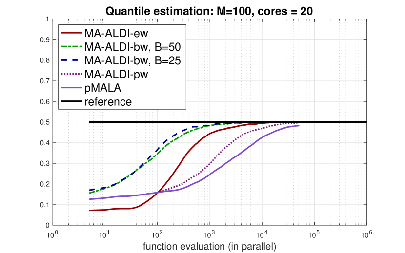
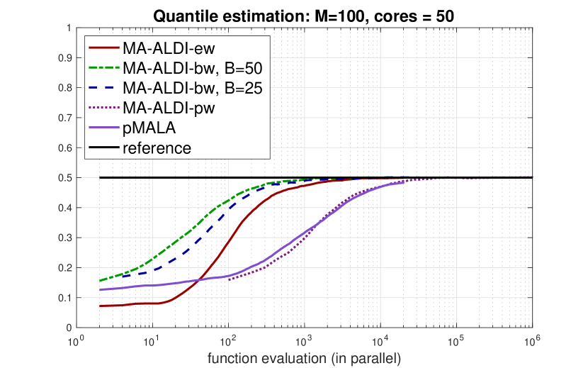
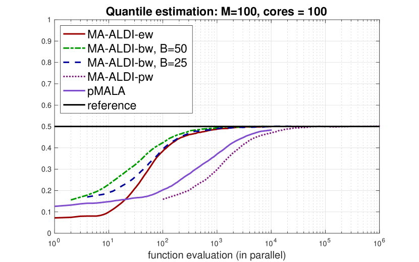
2. The second experiment is a more detailed study of MA-IPS using a four-dimensional multivariate Gaussian target distribution. It demonstrates the benefits of interaction (compared to independent parallel Markov chains) and compares the performance of all three Metropolization versions, in particular, under consideration of parallelization. Moreover, also the optimal tuning of the considered MA-IPS methods is studied empirically by the relation of the average acceptance rate and the obtained mean squared error of $\mathbf{S}^{M}_{N}(F)$ for a chosen $F$.

3. The final experiment applies the MA-IPS methods to a high-dimensional target distribution and confirms our observations in the low-dimensional setting.

We adhere to the following naming conventions for our algorithms:

• ALDI corresponds to the chain generated by (44), CBS corresponds to the chain generated by (48), and SVGD corresponds to the chain generated by (50),

• pMALA corresponds to parallel MALA, i.e. to $M$ independent chains each generated by Algorithm 2 with proposal (43),

• we use the prefix MA, to indicate that it’s the Metropolized version of an algorithm,

• we use the suffix ew to indicate ensemble-wise Metropolization as in Algorithm 3, e.g. MA-ALDI-ew corresponds to Algorithm 3 with proposal (44),

• we use the suffix pw to indicate particle-wise sequential Metropolization as in Algorithm 4, e.g. MA-ALDI-pw corresponds to Algorithm 4 with proposal (44),

• we use the suffix bw to indicate block-wise Metropolization as in Algorithm 5, e.g. MA-ALDI-bw corresponds to Algorithm 5 with proposal (44).

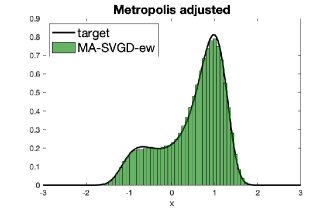
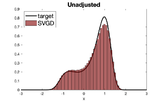
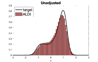
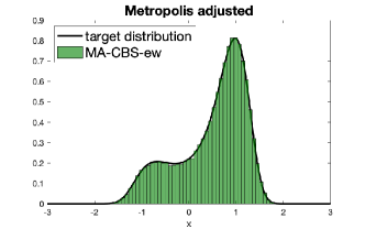
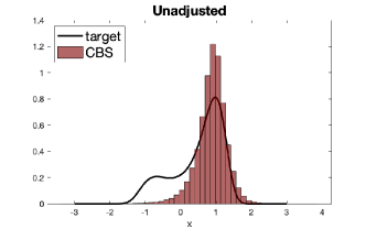
5.1 One-dimensional example: bimodal distribution

We study the effect of Metropolization on interacting particle systems for ALDI, CBS, and SVGD, by comparing the performance of each method with and without ensemble Metropolization.

As a target we consider the (unnormalized) probability density

$$\pi(x)\propto\exp\left(-\frac{1}{2\sigma^{2}}|x^{2}-1|^{2}\right)\cdot\exp\left(-\frac{1}{2}|x-m_{0}|^{2}\right)\qquad x\in\mathbb{R},$$

with $\sigma=0.1$ and $m_{0}=0.8$. This target density corresponds to a BIP with Gaussian prior distribution $\mathrm{N}(m_{0},1)$, forward model $G(x)=x^{2}$ and additive Gaussian noise with zero mean and variance $\sigma^{2}$.

For each particle sampling method we have simulated $N_{\mathrm{burn}}=10^{4}$ iterations of burn-in followed by another $N=10^{5}$ iterations. Both, the Metropolis-adjusted and unadjusted variant, were implemented with $M=10$ particles, same realization of the iid initialization $X_{0}^{(j)}\sim\mathrm{N}(m_{0},1)$, $j=1,\dots,M$ and same step size $h>0$ in the Euler-Maruyama scheme. For both ALDI versions we used step size $h=0.0725$ and for both CBS versions the step size $h=0.05$. For both SVGD versions we used step size $h=0.0001$ and the Gaussian kernel

$$k_{s}(x_{1},x_{2})=\exp\left(-\frac{1}{2s^{2}}|x_{1}-x_{2}|^{2}\right)$$

with $s=0.01$.

In Figure 1–3 we compare the histograms of the particles obtained by the Metropolis-adjusted and unadjusted algorithms accumulated over all $N$ iterations. For all three interactive particle methods, their unadjusted version do not seem to yield a sample from the target $\pi$ whereas their Metropolized versions do.

Figure 1: Comparison of MA-SVGD-ew and SVGD with $M=10$ particles and step size $h=0.0001$. MA-SVGD-ew achieved an acceptance rate of $53\%$.

Figure 2: Comparison of MA-ALDI-ew and ALDI with $M=10$ particles and step size $h=0.0725$. MA-ALDI-ew achieved an acceptance rate of $70\%$.

Figure 3: Comparison of MA-CBS-ew and CBS with $M=10$ particles and step size $h=0.05$. MA-CBS-ew achieved an acceptance rate of $52\%$.

5.2 Multivariate Gaussian distribution

We now consider a $4$-dimensional multivariate Gaussian target distribution $\mathrm{N}(0,C)$ with target density

$$\pi(x)\propto\exp\left(-\frac{1}{2}\|C^{-1/2}x\|^{2}\right),\qquad C=\operatorname{diag}(1,0.1,0.01,0.001).$$

As the coordinates are weighted differently, we expect a positive effect from the ensemble preconditioner. In this section we illustrate the benefits of interaction, compare ensemble-wise to particle-wise Metropolization (for MA-ALDI), and consider optimal tuning of MA-ALDI, MA-CBS, and MA-SVGD by controlling the acceptance rate.

To this end, we consider the quantity of interest $f(x)=x^{\top}C^{-1}x$ where for $X\sim\pi$ we have $f(X)\sim\chi^{2}(4)$. Our goal is then to estimate

$$P_{\mathrm{ref}}:=\mathbb{P}(f(X)\leq q_{0.5})=\mathbb{E}_{\pi}\left[\mathds{1}_{(-\infty,q_{0.5}]}(f(X))\right]=\frac{1}{2}$$ (51)

where $q_{0.5}$ denotes the $0.5$-quantile of the $\chi^{2}(4)$ distribution and $\mathds{1}_{A}$ the indicator function of a set $A$. The corresponding estimators based on ensemble Markov chains $(\boldsymbol{X}_{k})_{k\in\mathbb{N}}$ are then

$$\widehat{P}_{N}:=\frac{1}{N}\sum_{k=1}^{N}\mathbf{F}(\boldsymbol{X}_{k}),\qquad\mathbf{F}(\mathbf{x}):=\frac{1}{M}\sum_{i=1}^{M}\mathds{1}_{(-\infty,q_{0.5}]}(f(x^{(i)}))\in\mathbb{R}.$$

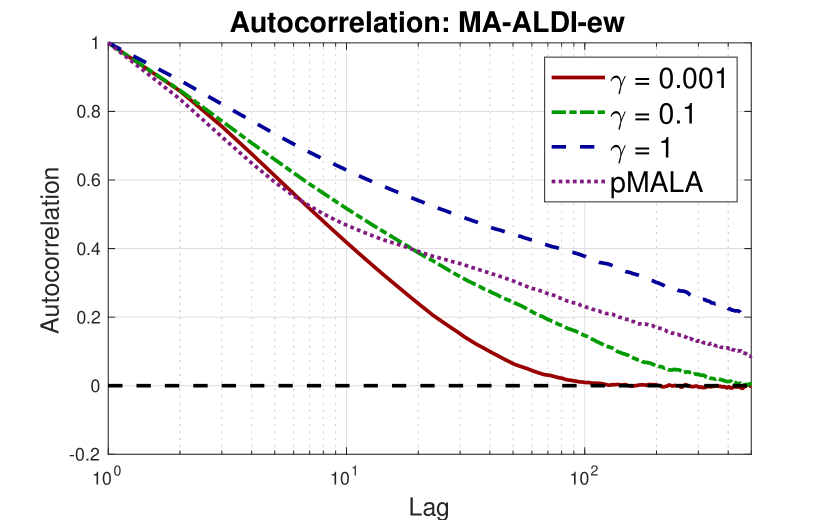
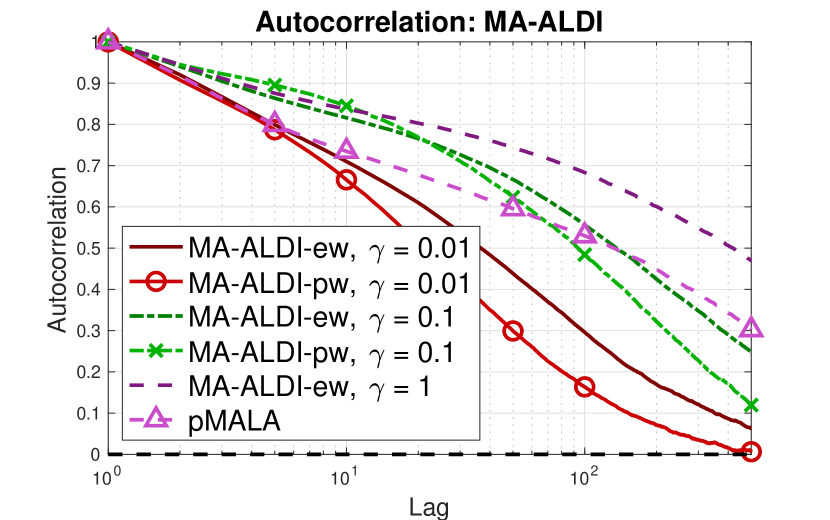
For evaluating the efficicency of these estimators we also compute the associated autocorrelations $\mathrm{Corr}(\mathbf{F}(\boldsymbol{X}_{1}),\mathbf{F}(\boldsymbol{X}_{1+k}))\approx\rho_{k}:=c_{k}/c_{0}$ where

$$c_{k}:=\frac{1}{N-k}\sum_{i=1}^{N-k}\left(\mathbf{F}(\boldsymbol{X}_{i})-\widehat{P}_{N}\right)\left(\mathbf{F}(\boldsymbol{X}_{i+k})-\widehat{P}_{N}\right)$$

since the $\rho_{k}$ yield information about the asymptotic variance (17) in the central limit theorem.

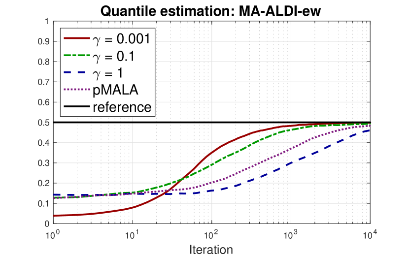
Superiority of interacting particles

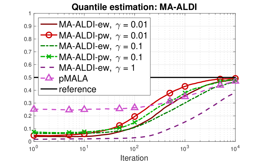
In Figure 4, we compare MA-ALDI-ew for different values of the covariance inflation parameter $\gamma\in\{0.001,0.1,1\}$ to pMALA, in order to show the improved performance for proposals generated by interacting particle systems. Note that for $\gamma=1$ the proposal of MA-ALDI-ew and pMALA are in fact the same, but MA-ALDI-ew uses ensemble-wise Metropolization while pMALA uses particle-wise Metropolization.

Figure 4(a) shows the evolution of $\widehat{P}_{N}$ averaged over $100$ independent runs for each method. For each method, we tuned the step size $h$ such that the average acceptance rate was around $50\%$. For $\gamma=0.001$ and $\gamma=0.1$ the MA-ALDI-ew based estimators converge much faster than pMALA. This observation is confirmed by the significantly faster decaying autocorrelation depicted on the right plot in Figure 4. On the other hand for $\gamma=1$ it is observed that MA-ALDI-ew performs worse than pMALA, suggesting that for $\gamma=1$ the particle-wise Metropolization is more effective than ensemble-wise Metropolization.

(a) quantile estimation

(b) autocorrelation

Figure 4: Estimation of $P_{\mathrm{ref}}$ in (51) and the corresponding estimated autocorrelation using either pMALA or MA-ALDI-ew for different choices of $\gamma$. For each method the step size $h$ was tuned to obtain an acceptance rate of approximately $50\%$.

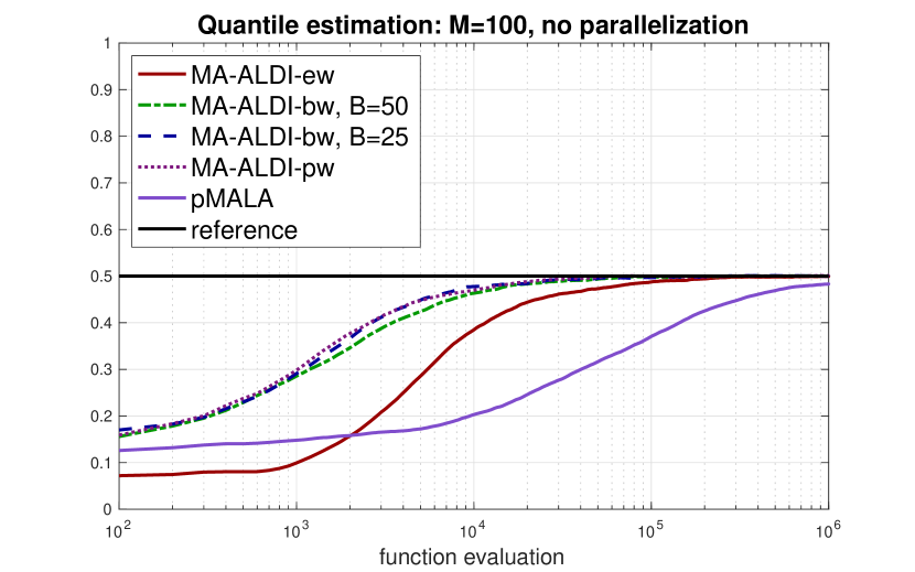
Superiority of particle- and block-wise Metropolization

In Figure 5 and Figure 6 we compare the ensemble-wise Metropolization MA-ALDI-ew with the particle- and block-wise Metropolizations MA-ALDI-pw and MA-ALDI-bw for $\gamma=0.001$. The results are obtained by averaging over $10$ independent runs of the corresponding methods. We used the same step size $h$ and ensemble size $M$ for all three MA-ALDI versions. Note that we have increased the ensemble size to $M=100$ in this experiment. Similar as for $\gamma=1$, the particle-wise Metropolization outperforms the ensemble-wise Metropolization also for $\gamma=0.001$ and $\gamma=0.1$. We see hardly any difference between particle- and block-wise Metropolization in Figure 5 (a), where we do not take into account possibilities for parallel computing. The result changes, when allowing access to multiple cores, such that the computation of the ensemble- and block-wise Metropolzation can be done in parallel. In Figure 5 (b) and Figure 6, we observe a clear advantage of block-wise and even ensemble-wise Metropolization the more cores we incorporate. In addition, Table 1 shows the estimated integrated autocorrelation scaled by the associated cost of the applied algorithm, i.e. the quantity

$${c({\mathrm{int\_ac}},B,{\mathrm{cores}})}={\mathrm{int}}\_{\mathrm{ac}}\cdot N\cdot M\cdot\frac{1}{\min\{\mathrm{cores},B\}}.$$ (52)

Here we assume all blocks in (40) to be of equal size $|\mathbf{b}_{j}|=B\in\mathbb{N}$ for all $j=1,\dots,L$ (and thus $M=LB$ is a multiple of $B$). Moreover, $\mathrm{cores}\in\mathbb{N}$ refers to the number of processors available for parallelization, $N$ is the number of iterations, and $\mathrm{int\_ac}$ refers to the estimated integrated autocorrelation. Note that ensemble-wise Metropolization and parallel MALA correspond to $B=M$ and particle-wise Metropolization corresponds to $B=1$.

cores	ew	bw, B=50	bw, B=25	pw	pMALA
$1$	$1366$	$840.6$	$708.1$	$593.2$	$8996$
$20$	$68.3$	$42$	$35.4$	$593.2$	$449.8$
$50$	$27.3$	$16.8$	$28.3$	$593.2$	$179.9$
$100$	$13.7$	$16.8$	$28.3$	$593.2$	$90$

Table 1: Comparison of the quantity in (52) measuring the computational efficiency of the method for different numbers of cores available and different variants of Metropolization.

(a) no parallelization

(b) 20 cores

Figure 5: Estimation of $P_{\mathrm{ref}}$ in (51) for different versions of MA-ALDI with $\gamma=0.001$, and pMALA. For MA-ALDI-ew the step size $h$ was tuned to obtain an acceptance rate of approximately $50\%$. For MA-ALDI-pw and both MA-ALDI-bw we use the same $h$ as for MA-ALDI-ew.

(a) 50 cores

(b) 100 cores

Figure 6: Same as Figure 5 but with different assumptions on accessible cores.

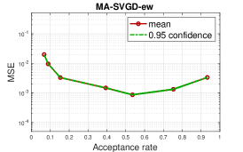
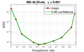
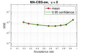
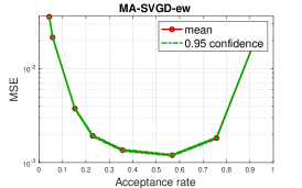
Optimal tuning

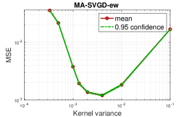
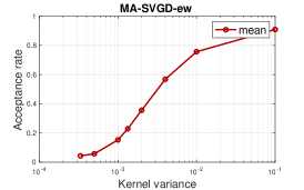
Finally, We study the dependence of the mean squared error (MSE) of $\mathbf{S}^{M}_{N}(F)$ on the average acceptance rate for the considered ensemble-wise MA-IPS in Figure 7. Here, we control the acceptance rate through the step size $h$ of the Euler-Maruyama scheme. The MSE was estimated over $100$ independent runs for each method and step size. We observe slightly different optimal average acceptance rates for MA-SVGD-ew, MA-ALDI-ew ($\gamma=0.001$), and MA-CBS-ew ($\gamma=0$), with MA-ALDI-ew notably performing most sensitive w.r.t. the acceptance rate, but also achieving the smallest MSE—by an order of magnitude smaller compared to MA-SVGD-ew and two orders of magnitude compared to MA-CBS-ew. For MA-SVGD-ew we can additionally control the acceptance rate through the kernel function: We use the Gaussian kernel

$$k_{s}(x_{1},x_{2})\propto\exp\left(-\frac{1}{2s^{2}}\|x_{1}-x_{2}\|^{2}\right),$$

and can also steer the performance of (MA-)SVGD by the variance parameter $s^{2}$. The results are shown in Figure 8. The optimal average acceptance rate seems to almost the same as for tuning $h$ (right). The dependence of the MSE and average acceptance rate is explicitly shown in the middle and right plot of Figure 8.

Figure 7: Comparison of the expected MSE depending on the expected acceptance rate for MA-SVGD-ew (left), MA-ALDI-ew with $\gamma=0.001$ (middle) and MA-CBS-ew with $\gamma=0$ (right).

Figure 8: Comparison of the expected MSE depending on the expected acceptance rate and the choice of kernel variance for MA-SVGD-ew.

5.3 ODE-based linear inverse problem

We consider the one-dimensional elliptic equation

$$\begin{cases}-\frac{{\mathrm{d}}^{2}p(s)}{{\mathrm{d}}^{2}s}+p(s)=\theta(s)&s\in D:=(0,1)\\ p(s)=0&s\in\{0,1\}\end{cases}$$ (53)

and the inverse problem of recovering the unknown right-hand side $\theta\in L^{\infty}(D)$ from noisy observations $y=A(\theta)+\xi\in\mathbb{R}^{K}$, where $\xi\in\mathbb{R}^{K}$ denotes observational noise. The forward operator $A:H^{-1}(D)\to\mathbb{R}^{K}$ is defined by

$$A=\mathcal{O}\circ G^{-1},\quad G=-\frac{{\mathrm{d}}^{2}}{{\mathrm{d}}^{2}s}+{\mathrm{id}}\ \text{on}\ \mathcal{D}(G)=H_{0}^{1}(D),$$

where $\mathcal{O}:H_{0}^{1}(D)\to\mathbb{R}^{K}$ denotes the observation operator providing function values of $K$ equidistant observation points $s_{k}=\frac{k}{K}$, $k=1,\dots,K$, such that for $p\in H_{0}^{1}(D)$ we have $\mathcal{O}p(\cdot)=(p(s_{1}),\dots,p(s_{K}))^{\top}$.

We consider a Gaussian process prior for $\theta$ given by

$$\theta(\cdot,x)=B_{\phi}x:=\sum_{i=1}^{d}x_{i}\phi_{i}(\cdot),$$

where $\phi_{i}(s)=\frac{\sqrt{2}}{\pi}\sin(i\pi s)$ and $x_{i}\sim\mathrm{N}(0,\lambda_{i})$ independently with $\lambda_{i}=i^{-2\tau}$ for some fixed $\tau>1$. Thus, the resulting inverse problem is to recover the coefficients $x=(x_{1},\dots,x_{d})^{\top}\in\mathbb{R}^{d}$ with prior information $\mathrm{N}(0,\Gamma_{0})$, where $\Gamma_{0}=\operatorname{diag}(\lambda_{1},\dots,\lambda_{d})$. Assuming additive Gaussian noise $\xi\sim\mathrm{N}(0,\Gamma)$ the resulting (unnormalized) posterior density is

$$\pi(x)\propto\exp\left(-\frac{1}{2}\|\Gamma^{-1/2}(y-AB_{\phi}x)\|^{2}-\frac{1}{2}\|\Gamma_{0}^{-1/2}x\|^{2}\right).$$

For the numerical implementation we replace $G$ by a numerical solution operator for (53) on the grid $D_{\delta}\subset D$ with mesh size $\delta=2^{-6}$ and restriction of the unknown parameter $\theta(\cdot,x)$ to $D_{\delta}$. We consider a fully observed system with $K=2^{6}$ and $d=10$ terms in the Gaussian process model.

We apply different versions of MA-ALDI with different choices of $\gamma\in\{0.01,0.1,1\}$ and compare them to pMALA. Note that the posterior $\pi$ is Gaussian with mean $m_{\ast}=\Gamma_{0}\tilde{A}^{\top}(\tilde{A}\Gamma_{0}\tilde{A}^{\top}+\Gamma)^{-1}y$ and covariance matrix $C_{\ast}=\Gamma_{0}-\Gamma_{0}\tilde{A}^{\top}(\tilde{A}\Gamma_{0}\tilde{A}^{\top}+ \Gamma)^{-1}\tilde{A}\Gamma_{0}\in\mathbb{R}^{d\times d}$ for $\tilde{A}:=AB_{\phi}\in\mathbb{R}^{K\times d}$. Therefore, we consider again the quantity of interest $f(X)=X^{\top}C_{\ast}^{-1}X\sim\chi^{2}(d)$, $X\sim\pi$, and the corresponding probability

$${P_{\mathrm{ref}}}=\mathbb{P}(f(X)\leq q_{0.5}),$$ (54)

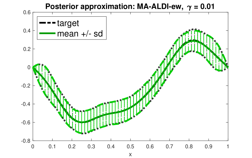
where $q_{0.5}$ denotes the $0.5$-quantile of the $\chi^{2}(d)$ distribution. We construct similar estimators of ${P_{\mathrm{ref}}}$ and the autocorrelation as in the previous section. The resulting estimation along the Markov chain and the estimated autocorrelation are plotted in Figure 9. Similar to before we report the average values of 100 independent runs for each method. Again, we observe that MA-ALDI outperforms pMALA. In particular, the particle-wise MA-ALDI with highest interaction ($\gamma=0.01$) performs best among all considered algorithms.

(a) quantile estimation

(b) autocorrelation

Figure 9: Estimation of $P_{\mathrm{ref}}$ in (54) and the corresponding estimated autocorrelation for different versions of MA-ALDI and $\gamma$, and pMALA. For MA-ALDI-ew and pMALA the step size $h$ was tuned to obtain an acceptance rate of approximately $50\%$. For MA-ALDI-pw we use the same $h$ as for MA-ALDI-ew.

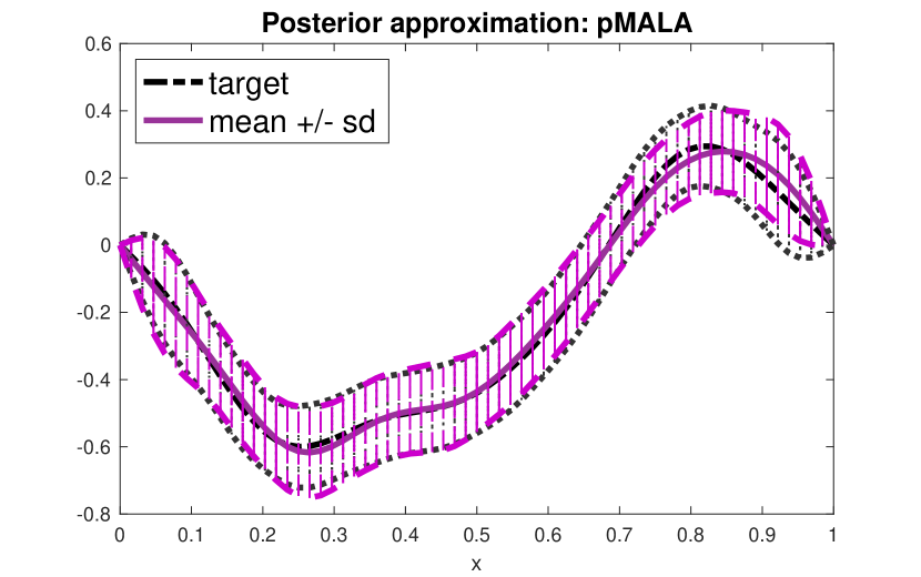
Moreover, we show the resulting posterior approximation averaged over the realized Markov chains pushed forward through the truncated KL-expansion, i.e., $\widehat{\theta}_{k}=B_{\phi}\boldsymbol{X}_{k}$. In Figure 10 we plot the pointwise mean $\frac{1}{N}\sum_{k=N_{\mathrm{burn}}}^{N_{\mathrm{burn}}+N}\widehat{\theta}_{k}$ plus/minus the pointwise empirical standard deviation. Here, we used again a burn-in of $N_{\mathrm{burn}}=10^{3}$ iterations and $N=10^{4}$ and observe a smaller deviation to true posterior for MA-ALDI-ew ($\gamma=0.01$) than for pMALA.

(a) MA-ALDI-ew

(b) pMALA

Figure 10: Posterior approximation (averaged over all iterations) for MA-ALDI-ew with $\gamma=0.01$ and pMALA. The step size $h$ was chosen such that the acceptance rate is approximately $50\%$.

6 Conclusion

The success of MCMC methods, particularly in high-dimensional problems, heavily relies on the quality of the proposal distribution. Ideally, additional information on the target distribution, such as its covariance, should be used. While this is not available in practice, it can for example be estimated along the path of the chain which has led to the developement of adaptive MCMC methods. In the present work, we consider an alternative approach that evolves an ensemble of $M\in\mathbb{N}$ interacting particles and leverages the information gained by the entire ensemble to generate a proposal for the next update. One key advantage is that this method provides an effective and natural means of parallelization which takes full advantage of the additional information provided by the ensemble. This can be crucial in the treatment of real-world problems. For instance, in engineering and science, solving a (Bayesian) inverse problems often involves simulating a complex physical process at each step of the chain. Each of these simulations can take minutes or even hours to complete, which renders any sequential algorithm and any MCMC approach that mixes only slowly infeasible.

The present study investigated three fundamental variants of Metropolizing interacting particle systems that evolve $M\in\mathbb{N}$ particles based on some stochastic ODE. The first variant considers the update as a proposal for the product of the target distribution in the product state space $\mathbb{R}^{Md}$. It either accepts or rejects the entire ensemble. The second variant employs particle-wise Metropolization, where each particle is accepted or rejected individually and sequentially. To allow for parallelization, in the third variant we partition the ensembles into blocks of equal size and sequentially accept or reject each block. While variant two has been proposed and discussed previously, e.g., in [7, 10, 14, 22], variants one and three are novel to the best of our knowledge. Furthermore, all three variants allow for the construction of affine-invariant MCMC methods through affine-invariant particle dynamics.

We presented a detailed empirical study comparing these methods for several common particle dynamics. Our findings show that the interaction of the particles can significantly improve mixing compared to trivially running $M$ independent MCMC chains (in parallel). Moreover, depending on the situation, we observed that the particle- and block-wise Metropolization seem to outperform the ensemble-wise variant. Overall, our study suggests that proposals based on interacting particle systems can provide significant improvements over traditional MCMC methods. Additionally, we provide a theoretical analysis of these methods, establishing basic ergodicity under mild and common assumptions. Finally, in the appendix we also discuss a “simultaneous” (instead of sequential) variant, and show why it does in general not yield the correct invariant distribution. Potential modifications to fix this biasedness are left as an open question for future work.

Other possible directions for future work include additionally using the history of the Markov chain, e.g., estimating the target covariance also along the path of the ensemble chain which may reduce the estimation error for the covariance. Also the application of localization techniques as discussed e.g., in [17, 33] within the MA-IPS approach seems beneficial. Finally, while we provide basic convergence results, a solid theoretical analysis of the superiority of interacting ensembles over independent, parallel Markov chains remains an open and interesting avenue for future work.

Acknowledgements

We thank Daniel Rudolf for very helpful and enduring discussions.

Appendix A On simultaneous particle-wise Metropolization

From a computational viewpoint, it would be advantegous to decide for each particle independently and in parallel whether to accept or reject it, as this facilitates the embarassingly parallel processing of all $M$ particles in the ensemble in each step of the algorithm. However, as we illustrate in the following, the corresponding “simultaneous” transition kernel is in general not invariant with respect to the product target measure $\boldsymbol{\pi}$ or even an $M$-coupling of $\pi$.

To formalize the outlined procedure, we consider the independent and simultaneous application of the particle-wise transition kernel $P_{\mathbf{x}^{-(i)}}$ in (33) to the $i$th particle for each $i\in\{1,\dots,M\}$. This yields the transition kernel $\mathbf{P}_{\mathrm{sim}}\colon\mathbb{R}^{Md}\times\mathcal{B}(\mathbb{R}^{Md})\to[0,1]$

$$\mathbf{P}_{\mathrm{sim}}(\mathbf{x},\mathrm{d}\mathbf{y})=P_{\mathbf{x}^{-(1)}}(x^{(1)},\mathrm{d}y^{(1)})\otimes\cdots\otimes P_{\mathbf{x}^{-(M)}}(x^{(M)},\mathrm{d}y^{(M)}).$$ (55)

The associated algorithmic description is given in Algorithm 6.

1:Input:

• target density $\pi$ on $\mathbb{R}^{d}$

• ensemble dependent proposal kernel $Q_{\mathbf{x}^{-}}$ with density $q_{\mathbf{x}^{-}}:\mathbb{R}^{d}\times\mathbb{R}^{d}\to(0,\infty)$ in (31)

• initial probability distribution $\pi_{0}$ on $\mathbb{R}^{d}$

2:Output: ensemble Markov chain $(\boldsymbol{X}_{k})_{k\in\{1,\dots,N\}}$ in state space $\mathbb{R}^{Md}$

3:draw $\mathbf{x}_{0}\sim\otimes_{i=1}^{M}\pi_{0}$ and set initial state $\boldsymbol{X}_{0}=\mathbf{x}_{0}\in\mathbb{R}^{Md}$

4:for $k=0,\dots,N$ do

5:     $\forall i$: given $\boldsymbol{X}_{k}=\mathbf{x}_{k}$ draw proposal $y^{(i)}\sim Q_{\mathbf{x}^{-(i)}_{k}}(x^{(i)}_{k},\cdot)$ independently

6:     $\forall i$: compute particle acceptance probability $\alpha_{\mathbf{x}^{-(i)}_{k}}(x^{(i)}_{k},y^{(i)})\in[0,1]$ in (32)

7:     $\forall i$: draw $u_{i}\sim{\rm U}([0,1])$ independently and set

$$X^{(i)}_{k+1}=\begin{cases}y^{(i)}&\text{if }u_{i}\leq\alpha_{\mathbf{x}^{-(i)}_{k}}(x^{(i)}_{k},y^{(i)})\\ x_{k}^{(i)}&\text{else}\end{cases}$$

8:end for

Algorithm 6 Simultaneous particle-wise Metropolized interactive particle sampling

As for the sequential updates discussed in Section 3.2 and 3.3, $\boldsymbol{\pi}$-reversibility does not hold, since in general

$$\prod_{i=1}^{M}\left(\alpha_{\mathbf{x}^{-(i)}}(x^{(i)},y^{(i)})\,q_{\mathbf{x}^{-(i)}}(x^{(i)},y^{(i)})\,\pi(x^{(i)})\right)\neq\prod_{i=1}^{M}\left(\alpha_{\mathbf{y}^{-(i)}}(y^{(i)},x^{(i)})\,q_{\mathbf{y}^{-(i)}}(y^{(i)},x^{(i)})\,\pi(y^{(i)})\right)$$

for $\mathbf{x}$, $\mathbf{y}\in\mathbb{R}^{Md}$ with $x^{(i)}\neq y^{(j)}$ for all $i,j=1,\ldots,M$—except for the case of noninteraction, i.e., $q_{\mathbf{x}^{-}}=q$ and, thus, $\alpha_{\mathbf{x}^{-}}=\alpha$ does not depend on the other particles in the ensemble.

Regarding the $\boldsymbol{\pi}$ invariance of $\mathbf{P}_{\rm sim}$, it is worth noting that each $P_{\mathbf{x}^{-(i)}}$ is $\pi$-invariant. However, due to the interaction, this does not directly imply $\boldsymbol{\pi}$ invariance of $\mathbf{P}_{\rm sim}$. Although, the particle-wise marginals of $\boldsymbol{\pi}$ and $\boldsymbol{\pi}\mathbf{P}_{\mathrm{sim}}$ coincide as shown below in Proposition A.1 the product transition kernel $\mathbf{P}_{\mathrm{sim}}$ is in general not $\boldsymbol{\pi}$ invariant as illustrated by several counterexamples below.

Proposition A.1.

For the transition kernel $\mathbf{P}_{\mathrm{sim}}\colon\mathbb{R}^{Md}\times\mathcal{B}(\mathbb{R}^{Md})\to[0,1]$ given in (55) associated to Algorithm 6 we have that $\boldsymbol{\pi}\mathbf{P}_{\mathrm{sim}}$ is an $M$-coupling of $\pi$, i.e. the particle-wise marginals of $\boldsymbol{X}\sim\boldsymbol{\pi}\mathbf{P}_{\mathrm{sim}}$ are $X^{(i)}\sim\pi$ for all $i=1,\ldots,M$.

Proof.

For any $i=1,\ldots,M$ and any $A_{i}\in\mathcal{B}(\mathbb{R}^{d})$ we have

$$\boldsymbol{\pi}\mathbf{P}_{\mathrm{sim}}(\mathbb{R}^{d}\times\cdots\times\mathbb{R}^{d}\times A_{i}\times\mathbb{R}^{d}\times\cdots\times\mathbb{R}^{d}) =\int_{\mathbb{R}^{Md}}\mathbf{P}_{\mathrm{sim}}(\mathbf{x},\mathbb{R}^{d}\times\cdots\times\mathbb{R}^{d}\times A_{i}\times\mathbb{R}^{d}\times\cdots\times\mathbb{R}^{d})\,\boldsymbol{\pi}({\rm d}\mathbf{x})$$

$$=\int_{\mathbb{R}^{Md}}P_{\mathbf{x}^{-(i)}}(x^{(i)},A_{i})\,\,\boldsymbol{\pi}({\rm d}\mathbf{x})$$

$$=\int_{\mathbb{R}^{(M-1)d}}\left(\int_{\mathbb{R}^{d}}P_{\mathbf{x}^{-(i)}}(x^{(i)},A_{i})\,\pi({\rm d}x^{(i)})\right)\,\bigotimes_{j\neq i}\pi({\rm d}x^{(j)})$$

$$=\int_{\mathbb{R}^{(M-1)d}}\pi(A_{i})\,\bigotimes_{j\neq i}\pi({\rm d}x^{(j)})=\pi(A_{i})$$

due to the $\pi$-invariance of $P_{\mathbf{x}^{-}}$ for any $\mathbf{x}^{-}\in\mathbb{R}^{(M-1)d}$. ∎

Remark A.2.

If we assume $\boldsymbol{\pi}$-invariance of $\mathbf{P}_{\mathrm{sim}}$, then ergodicity and a strong law of large numbers follow under the same conditions as in Theorem 3.6; this can be proven by a slight modification of the arguments in [38].

Example A.3.

Let us consider a discrete state space $\mathcal{X}=\{x_{1},x_{2}\}$ of two elements $x_{1}\neq x_{2}$ and the uniform distribution $\pi(x_{1})=\pi(x_{2})=\frac{1}{2}$ on $\mathcal{X}$ as the target measure. Consider parametrized proposal kernels $Q_{z}\colon\mathcal{X}\times\mathcal{X}\to[0,1]$ with parameter $z\in\mathcal{X}$ which we write as right stochastic matrices $\mathrm{Q}_{z}\in[0,1]^{|\mathcal{X}|}$ where the element $q_{ij}$ of $\mathrm{Q}_{z}$ in the $i$th row and $j$th column denotes the probability $Q_{z}(x_{i},x_{j})$:

$$\mathrm{Q}_{x_{1}}=\begin{pmatrix}2/3&1/3\\ 2/3&1/3\end{pmatrix},\qquad\mathrm{Q}_{x_{2}}=\begin{pmatrix}1/2&1/2\\ 1/2&1/2\end{pmatrix}.$$

The resulting parametrized acceptance probabilities $\alpha_{z}\colon\mathcal{X}\times\mathcal{X}\to[0,1]$ are given by (cp. (18))

$$\alpha_{x_{1}}(x,y)=\begin{cases}1/2,&\text{if }x=x_{2},y=x_{1}\\ 1,&\text{else}\end{cases},\qquad\alpha_{x_{2}}(x,y)\equiv 1,$$

and the rejection probabilies by (cp. (19))

$$r_{x_{1}}(x)=\begin{cases}1/3,&x=x_{1}\\ 0,&x=x_{2}\end{cases},\qquad r_{x_{2}}(x)\equiv 0.$$

This yields as $\pi$-invariant MH transition kernel $P_{z}\colon\mathcal{X}\times\mathcal{X}\to[0,1]$ again written as right stochastic matrices $\mathrm{P}_{z}$ (cp. (19))

$$\mathrm{P}_{x_{1}}=\begin{pmatrix}2/3&1/3\\ 2/3&1/3\end{pmatrix},\qquad\mathrm{P}_{x_{2}}=\begin{pmatrix}1/2&1/2\\ 1/2&1/2\end{pmatrix}.$$

The resulting product transition kernel

$$\mathbf{P}_{\mathrm{sim}}(\mathbf{x},\mathbf{y})=P_{x^{(2)}}(x^{(1)},y^{(1)})\cdot P_{x^{(1)}}(x^{(2)},y^{(2)})$$

is then, written as well as a $(4\times 4)$-right stochastic matrix where the rows and columns in the matrix correspond to the lexicographically ordered states $(x_{1},x_{1}),(x_{1},x_{2}),(x_{2},x_{1}),(x_{2},x_{2})$ in $\mathcal{X}^{2}$,

$$\mathbf{P}_{\mathrm{sim}}\simeq\begin{pmatrix}4/9&2/9&2/9&1/9\\ 1/6&2/6&1/6&2/6\\ 1/6&2/6&1/6&2/6\\ 1/4&1/4&1/4&1/4\end{pmatrix}.$$

The associated invariant measure $\boldsymbol{\nu}\colon\mathcal{X}^{2}\to[0,1]$ is given by

$$\boldsymbol{\nu}(x_{1},x_{1})=\frac{45}{173},\quad\boldsymbol{\nu}(x_{1},x_{2})=\frac{49}{173},\quad\boldsymbol{\nu}(x_{2},x_{1})=\frac{35}{173},\quad\boldsymbol{\nu}(x_{2},x_{2})=\frac{44}{173}$$

which does not correspond to $\boldsymbol{\pi}\equiv\frac{1}{4}$. Moreover, also the particlewise marginals $\nu^{(i)}$ of $\boldsymbol{\nu}$ do not coincide with $\pi$:

$$\nu^{(1)}(x_{1})=\frac{94}{173},\quad\nu^{(1)}(x_{2})=\frac{79}{173},\qquad\nu^{(2)}(x_{1})=\frac{80}{173},\quad\nu^{(2)}(x_{2})=\frac{93}{173}.$$

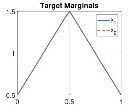
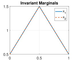
Example A.4.

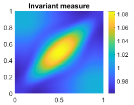
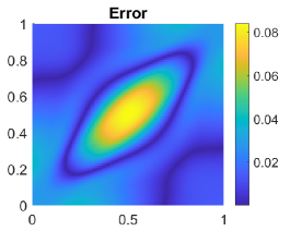
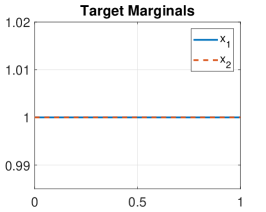
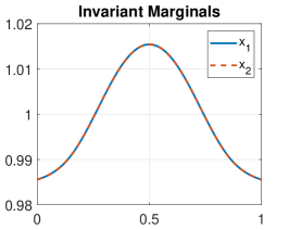
Let us consider the continuous state space $\mathcal{X}=\mathbb{R}$ equipped with the triangular target distribution $\pi$ given by the Lebesgue density

$$\pi(x)=\begin{cases}\frac{1}{2}+2\min\{x,1-x\},&\text{if }x\in[0,1]\\ 0,&\text{else.}\end{cases}$$

Again, we consider an ensemble Markov chain of $M=2$ interacting particles $\boldsymbol{X}_{k}=(X_{k}^{(1)},X_{k}^{(2)})^{\top}\in\mathbb{R}^{2}$. As ensemble proposal kernel we choose the following

$$\mathbf{Q}(\mathbf{x},{\rm d}\mathbf{y})=Q_{x^{(2)}}(x^{(1)},{\rm d}y^{(1)})\otimes Q_{x^{(1)}}(x^{(2)},{\rm d}y^{(2)}),\qquad Q_{z}(x,{\rm d}y)=\mathrm{N}\left(\frac{x+z}{2},\frac{1}{4}\right),$$

which corresponds particle-wise to $\mathrm{N}\left(m(\boldsymbol{X}_{k}),h\right)$ for $h=\frac{1}{4}$. Consider the transition kernel $\mathbf{P}_{\mathrm{sim}}$ resulting from particle-wise Metropolization. Note that for $M=2$ we can decompose $\mathbf{P}_{\mathrm{sim}}$ as follows

$$\mathbf{P}_{\mathrm{sim}}((x_{1},x_{2}),{\rm d}y_{1},{\rm d}y_{2}) =\alpha_{x_{2}}(x_{1},y_{1})\alpha_{x_{1}}(x_{2},y_{2})q_{x_{2}}(x_{1},y_{1})q_{x_{1}}(x_{2},y_{2}){\rm d}y_{1}{\rm d}y_{2}$$

$$\quad+\alpha_{x_{2}}(x_{1},y_{1})r_{x_{1}}(x_{2})q_{x_{2}}(x_{1},y_{1}){\rm d}y_{1}\delta_{x_{2}}({\rm d}y_{2})$$

$$\quad+r_{x_{2}}(x_{1})\alpha_{x_{1}}(x_{2},y_{2})q_{x_{1}}(x_{2},y_{2}){\rm d}y_{2}\delta_{x_{1}}({\rm d}y_{1})$$

$$\quad+r_{x_{2}}(x_{1})r_{x_{1}}(x_{2})\delta_{x_{1}}({\rm d}y_{1})\delta_{x_{2}}({\rm d}y_{2})$$

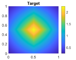
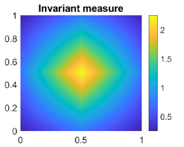
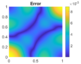
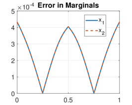
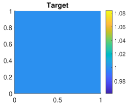
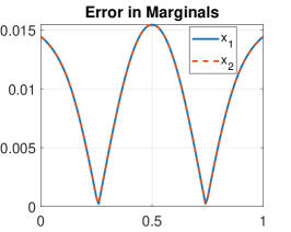
where $q_{z}$ denotes the Lebesgue density of $Q_{z}$. We then discretize the state space to obtain a transition matrix $\mathbf{P}_{\mathrm{sim}}\in\mathbb{R}^{n\times n}$ and compute its invariant measure as approximation to the true invariant measure of the operator $\mathbf{P}_{\mathrm{sim}}$. Since $\alpha_{z}(x,y)=0$ for $y\notin[0,1]$ it suffices to discretize $[0,1]^{2}$. Here we use a uniform grid with grid size $\Delta x=0.01$ in each dimension. Thus, $n=101^{2}$.The invariant measure of the matrix $\mathbf{P}_{\mathrm{sim}}\in\mathbb{R}^{n\times n}$ is then computed numerically and rearranged to yield $\boldsymbol{\pi}_{\text{inv}}\in[0,1]^{101\times 101}$. It is displayed in comparison to an analogously discretized version of the true product target $\boldsymbol{\pi}=\pi\otimes\pi$ in Figure 11. We do notice a bias, although a small one of relative size $10^{-3}$ to $10^{-2}$. Since the crucial object for sampling purposes is not necesarilly the invariant measure in the ensemble space but the particle-wise marginals of it we also compare these in Figure 12. However, the results are similar here. A small bias is observable, again the relative size compared to the true target are of order $10^{-3}$.

Figure 11: Comparison true product target and numerically computed invariant measure of simultaneous particle-wise Metropoliziation $\mathbf{P}_{\mathrm{sim}}$ for $M=2$ particles in Example A.4.

Figure 12: Comparison true product target and numerically computed invariant measure of simultaneous particle-wise Metropoliziation $\mathbf{P}_{\mathrm{sim}}$ for $M=2$ particles in Example A.4.

Example A.5.

We provide another numerical example similar to the previous one. Here again, $\mathcal{X}=\mathbb{R}$ but now $\pi=\mathbb{U}[0,1]$ is the uniform distribution on $[0,1]$. We consider $M=2$ interacting particles $\boldsymbol{X}_{k}=(X_{k}^{(1)},X_{k}^{(2)})^{\top}\in\mathbb{R}^{2}$ based on the following ensemble proposal kernel

$$\mathbf{Q}(\mathbf{x},{\rm d}\mathbf{y})=Q_{x^{(2)}}(x^{(1)},{\rm d}y^{(1)})\otimes Q_{x^{(1)}}(x^{(2)},{\rm d}y^{(2)}),\qquad Q_{z}(x,{\rm d}y)=\mathrm{N}\left(x,\frac{1}{4}\left(0.01+\frac{0.99}{2}(z-x)^{2}\right)\right)$$

which corresponds particle-wise to $\mathrm{N}\left(x,h(\gamma+(1-\gamma)C(\boldsymbol{X}_{k}))\right)$ with $\gamma=0.01$ and $h=\frac{1}{4}$. Analogously, we discretize the state space or $[0,1]^{2}$, respectively, using a uniform grid with grid size $\Delta x=0.01$ and compute numerically the invariant measure of the resulting transition matrix $\mathbf{P}_{\mathrm{sim}}\in\mathbb{R}^{101\times 101}$. The results are shown in Figure 13 and 14. Also for this example we do notice a bias which is even larger than in the previous example, i.e., we observe a relative error of order $10^{-2}$ to $10^{-1}$ for the joint target and $10^{-2}$ for the particle-wise marginals.

Figure 13: Comparison true product target and numerically computed invariant measure of simultaneous particle-wise Metropoliziation $\mathbf{P}_{\mathrm{sim}}$ for $M=2$ particles in Example A.5.

Figure 14: Comparison true product target and numerically computed invariant measure of simultaneous particle-wise Metropoliziation $\mathbf{P}_{\mathrm{sim}}$ for $M=2$ particles in Example A.5.

We suspect that the bias of simultaneous particle-wise Metropolization is larger for smaller ensemble sizes than for bigger ones. In particular, the bias may vanish as $M\to\infty$ for suitable interacting particle systems, i.e., if the dynamics of each particle converge to their only time-discretized mean field limit as $M\to\infty$, then the corresponding proposal distributions $Q_{x^{-(i)}}(x^{(i)},\cdot)$ should also converge to a limit proposal distribution $Q_{\infty}(x^{(i)},\cdot)$ which does not depend on the other particles anymore, e.g., $Q_{\infty}(x^{(i)},\cdot)=\mathrm{N}(x^{(i)}+hC(\pi_{t})\nabla\log\pi(x^{i}),2hC(\pi_{t}))$ in case of ALDI. However, for independent proposal kernels $Q_{x^{-(i)}}(x^{(i)},\cdot)=Q(x^{(i)},\cdot)$ the transition kernel of simultaneous particle-wise Metropolization $\mathbf{P}_{\mathrm{sim}}$ is in fact $\boldsymbol{\pi}$-invariant. Therefore, we suspect that the bias of $\mathbf{P}_{\mathrm{sim}}$ is largest for the $M=2$ particle case considered in the numerical counterexamples above.

References

- [1] J. Besag. Discussion of “Representations of knowledge in complex systems”. J. Roy. Statist. Soc. Ser. B, 56(4):591–592, 1994.
- [2] S. Brooks, A. Gelman, G. Jones, and X.-L. Meng (Eds.). Handbook of Markov Chain Monte Carlo. Chapman and Hall/CRC, New York, NY, 2011.
- [3] J. A. Carrillo, F. Hoffmann, A. M. Stuart, and U. Vaes. Consensus-based sampling. Studies in Applied Mathematics, 148(3):1069–1140, 2022.
- [4] R. T. Q. Chen, Y. Rubanova, J. Bettencourt, and D. K. Duvenaud. Neural ordinary differential equations. In S. Bengio, H. Wallach, H. Larochelle, K. Grauman, N. Cesa-Bianchi, and R. Garnett, editors, Advances in Neural Information Processing Systems, volume 31. Curran Associates, Inc., 2018.
- [5] J. A. Christen and C. Fox. A general purpose sampling algorithm for continuous distributions (the t-walk). Bayesian Analysis, 5(2):263 – 281, 2010.
- [6] S. Cotter, G. Roberts, A. Stuart, and D. White. MCMC methods for functions: Modifying old algorithms to make them faster. Statistial Science, 28(3):283–464, 2013.
- [7] J. Coullon and R. J. Webber. Ensemble sampler for infinite-dimensional inverse problems. Statistics and Computing, 31:28, 2021.
- [8] S. Dolgov, K. Anaya-Izquierdo, C. Fox, and R. Scheichl. Approximation and sampling of multivariate probability distributions in the tensor train decomposition. Stat. Comput., 30(3):603–625, 2020.
- [9] A. Duncan, N. Nuesken, and L. Szpruch. On the geometry of Stein variational gradient descent. ArXiv, abs/1912.00894, 2019.
- [10] M. M. Dunlop and G. Stadler. A gradient-free subspace-adjusting ensemble sampler for infinite-dimensional Bayesian inverse problems. ArXiv, abs/2202.11088, 2022.
- [11] V. Gallego and D. R. Insua. Stochastic gradient MCMC with repulsive forces. ArXiv, abs/1812.00071, 2018.
- [12] A. Garbuno-Inigo, F. Hoffmann, W. Li, and A. M. Stuart. Interacting Langevin diffusions: gradient structure and ensemble Kalman sampler. SIAM Journal on Applied Dynamical Systems, 19(1):412–441, 2020.
- [13] A. Garbuno-Inigo, N. Nüsken, and S. Reich. Affine invariant interacting Langevin dynamics for Bayesian inference. SIAM Journal on Applied Dynamical Systems, 19(3):1633–1658, 2020.
- [14] J. Goodman and J. Weare. Ensemble samplers with affine invariance. Comm. App. Math. and Comp. Sci., (1), 2010.
- [15] U. Grenander and M. I. Miller. Representations of knowledge in complex systems. J. Roy. Statist. Soc. Ser. B, 56(4):549–603, 1994.
- [16] W. K. Hastings. Monte Carlo sampling methods using Markov chains and their applications. Biometrika, 57(1):97–109, 1970.
- [17] D. Z. Huang, J. Huang, S. Reich, and A. M. Stuart. Efficient derivative-free Bayesian inference for large-scale inverse problems. Inverse Problems, 38(12):125006, oct 2022.
- [18] M. A. Iglesias, K. J. H. Law, and A. M. Stuart. Ensemble Kalman methods for inverse problems. Inverse Problems, 29(4):045001, mar 2013.
- [19] P. Jaini, K. A. Selby, and Y. Yu. Sum-of-squares polynomial flow. ICML, 2019.
- [20] R. Jordan, D. Kinderlehrer, and F. Otto. The variational formulation of the Fokker–Planck equation. SIAM Journal on Mathematical Analysis, 29:1–17, 1998.
- [21] A. Korba, A. Salim, M. Arbel, G. Luise, and A. Gretton. A non-asymptotic analysis for Stein variational gradient descent. In Advances in Neural Information Processing Systems, volume 33, pages 4672–4682. Curran Associates, Inc., 2020.
- [22] B. Leimkuhler, C. Matthews, and J. Weare. Ensemble preconditioning for Markov chain Monte Carlo simulation. Statistics and Computing, 28(2):277–290, 2018.
- [23] Q. Liu. Stein variational gradient descent as gradient flow. In Advances in Neural Information Processing Systems 30, pages 3115–3123. Curran Associates, Inc., 2017.
- [24] Q. Liu and D. Wang. Stein variational gradient descent: A general purpose Bayesian inference algorithm. In Proceedings of the 30th International Conference on Neural Information Processing Systems, NIPS’16, page 2378–2386, Red Hook, NY, USA, 2016. Curran Associates Inc.
- [25] P. A. Markowich and C. Villani. On the trend to equilibrium for the Fokker-Planck equation: an interplay between physics and functional analysis. volume 19, pages 1–29. 2000. VI Workshop on Partial Differential Equations, Part II (Rio de Janeiro, 1999).
- [26] Y. Marzouk, T. Moselhy, M. Parno, and A. Spantini. Sampling via measure transport: an introduction. In Handbook of uncertainty quantification. Vol. 1, 2, 3, pages 785–825. Springer, Cham, 2017.
- [27] N. Metropolis, A. W. Rosenbluth, M. N. Rosenbluth, A. H. Teller, and E. Teller. Equation of State Calculations by Fast Computing Machines. J. Chem. Phys., 21(6):1087–1092, June 1953.
- [28] N. Nüsken and S. Reich. Note on interacting Langevin diffusion: Gradient structure and ensemble Kalman sampler. Technical Report arXiv:1908.10890v1, University of Potsdam, 2019.
- [29] N. Nüsken and D. R. M. Renger. Stein variational gradient descent: Many-particle and long-time asymptotics. Foundations of Data Science, 2023.
- [30] S. Pathiraja, S. Reich, and W. Stannat. Mckean–Vlasov SDEs in nonlinear filtering. SIAM Journal on Control and Optimization, 59(6):4188–4215, 2021.
- [31] G. Pavliotis. Stochastic Processes and Applications: Diffusion Processes, the Fokker-Planck and Langevin Equations. Texts in Applied Mathematics. Springer New York, 2014.
- [32] R. Pinnau, C. Totzeck, O. Tse, and S. Martin. A consensus-based model for global optimization and its mean-field limit. Mathematical Models & Methods in Applied Sciences, 27(1):183–204, 2017.
- [33] S. Reich and S. Weissmann. Fokker–Planck particle systems for Bayesian inference: Computational approaches. SIAM/ASA Journal on Uncertainty Quantification, 9(2):446–482, 2021.
- [34] D. Rezende and S. Mohamed. Variational inference with normalizing flows. In F. Bach and D. Blei, editors, Proceedings of the 32nd International Conference on Machine Learning, volume 37 of Proceedings of Machine Learning Research, pages 1530–1538, Lille, France, 07–09 Jul 2015. PMLR.
- [35] C. P. Robert and G. Casella. Monte Carlo Statistical Methods. Texts in Statistics. Springer New York, 2004.
- [36] G. O. Roberts and J. S. Rosenthal. Optimal scaling for various Metropolis–Hastings algorithms. Statistical Science, 16(4):351–367, 2001.
- [37] G. O. Roberts and J. S. Rosenthal. General state space Markov chains and MCMC algorithms. Probability Surveys, 1:20–71, 2004.
- [38] G. O. Roberts and J. S. Rosenthal. Harris recurrence of Metropolis-within-Gibbs and trans-dimensional Markov chains. Annals of Applied Probability, 16(4):2123–2139, 2006.
- [39] G. O. Roberts and R. L. Tweedie. Exponential convergence of Langevin distributions and their discrete approximations. Bernoulli, 2(4):341–363, 1996.
- [40] D. Rudolf and B. Sprungk. On a generalization of the preconditioned Crank–Nicolson Metropolis algorithm. Found. Comput. Math., 18:309–343, 2018.
- [41] D. Rudolf and B. Sprungk. Robust random walk-like Metropolis–Hastings algorithms for concentrating posteriors. arXiv:2202.12127, 2022.
- [42] S. Vempala and A. Wibisono. Rapid convergence of the unadjusted Langevin algorithm: Isoperimetry suffices. In H. Wallach, H. Larochelle, A. Beygelzimer, F. d'Alché-Buc, E. Fox, and R. Garnett, editors, Advances in Neural Information Processing Systems, volume 32. Curran Associates, Inc., 2019.
- [43] S. Weissmann. Gradient flow structure and convergence analysis of the ensemble Kalman inversion for nonlinear forward models. Inverse Problems, 38(10):105011, sep 2022.