Quantum Wave Function Collapse
for Procedural Content Generation

Abstract

Quantum computers exhibit an inherent randomness, so it seems natural to consider them for procedural content generation. In this work, a quantum version of the famous (classical) wave function collapse algorithm is proposed. This quantum wave function collapse algorithm is based on the idea that a quantum circuit can be prepared in such a way that it acts as a special-purpose random generator for content of a desired form. The proposed method is presented theoretically and investigated experimentally on simulators and actual IBM Quantum devices.

Wave function collapse (WFC) is a powerful tool for procedural content generation (PCG) that is for example used in video games, as it can save significant development time by automating the creation of diverse and complicated game elements. However, it is not limited to video games, but also has applications in various other fields, including art and design, where the need for algorithmically generated content is widespread. Content in this context can therefore have a broad range of meanings: Images, 3D models, game levels, text, sound or a combination of these, to name just a few examples.

Originally proposed in Ref. [1], the WFC algorithm is a a non-backtracking, greedy constraint solving method [2, 3] that is able to generate complex patterns based on a set of input samples. It is known for its ability to create diverse and complex outputs that resemble the input samples while exhibiting novel combinations and variations. WFC employs two implementation strategies: the simple tiled model and the overlapping model, which share an identical algorithm core [4]. In the simple tiled model, tilesets are manually prescribed with predefined adjacency constraints, whereas the overlapping model automatically generates this information from a sample input.

In both strategies, the output is compartmentalized into segments and the possibilities for each segment are iteratively constrained until a unique solution is determined. The term “wave function collapse” is borrowed from quantum physics because of the conceptual similarity. The “wave function” refers to the set of potential states of the segments, whereas the ”collapse“ occurs during the iterative process of narrowing down the possibilities.

Despite its name, WFC is a purely classical algorithm. But even if WFC has nothing to do with quantum physics beyond the terminology, the question naturally arises as to whether quantum computers can be used to execute a genuine quantum version of the algorithm. The investigation of this question and a first draft for a corresponding algorithm are the subject of this manuscript. For this purpose, the terms classical wave function collapse (CWFC), quantum wave function collapse (QWFC), and hybrid quantum-classical wave function collapse (HWFC) are used In the following to clearly distinguish between classical, quantum and hybrid quantum-classical WFC.

Leveraging quantum computers for PCG has been considered before, mainly focusing on the quantum generalization of a blurring process [5, 6] and map generation using a quantum-enhanced decision making process [7]. Related projects have been carried out in connection with the development of quantum-inspired games [8].

The contribution of this paper is threefold:

• A probabilistic formulation of the simple tiled model of CWFC is presented as a foundation for a quantum version.

• A QWFC method and a HWFC method are proposed.

• The proposed methods are tested on simulators and actual IBM Quantum devices.

The remaining manuscript is structured as follows. In the next section, a formal description of CWFC is provided in an appropriate probabilistic form, which enables the development of a QWFC method and a HWFC method in the subsequent section. In the section after, the proposed methods are demonstrated in practice. Finally, the paper ends with a conclusion and an outlook.

1 CLASSICAL METHODS

In this section, the formal description for a probabilistic iterative PCG (PIPCG) is provided and, subsequently, it is shown how it can be reduced to the common CWFC approach.

1.1 PIPCG

To begin with, it is first necessary to formally define the generated content at a sufficiently abstract level. For this purpose, it is presumed that any content instance $C$ can be described as an ordered sequence of $N$ segments

$$C:=\{(1,v_{1}),\dots,(N,v_{N})\}\in\mathcal{C},$$ (1)

where each segment $(i,v_{i})$ is defined by a unique identifier $i\in[1,N]$ and a value $v_{i}\in A_{i}$ from an alphabet $A_{i}\subset\mathbb{N}$. Here and in the following, the notation $[i,j]:=\{i,\dots,j\}\,\forall\,i,j\in\mathbb{N}$ is used. The set of all possible content instances $\mathcal{C}$ is determined by the content alphabets $\mathcal{A}:=\{A_{1},\dots,A_{N}\}$ for a given size $N$ with $|\mathcal{C}|=\prod_{i=1}^{N}A_{i}$. For example, if the content represents an image, its individual pixels can constitute the segments. Each pixel can attain one color from the available color space of the image (as its alphabet).

1.1.1 Iterative process.

The procedural generation of content instance $C\in\mathcal{C}$ is realized through an iterative process, where each iteration $k\in[1,N]$ consists of three steps:

1. Randomly choose a new segment identifier $s(k)\in[1,N]$ from a set of available identifiers.

2. Randomly choose a corresponding value $v_{s(k)}\in A_{s(k)}$ from a set of available values.

3. Add the chosen segment $(s(k),v_{s(k)})$ to the content instance.

By repeating these steps, the content instance is assembled in the sense of $C(0)\overset{k=1}{\rightarrow}C(1)\overset{k=2}{\rightarrow}\cdots\overset{k=N}{\rightarrow}C(N)$, where

$$C(k):=\{(s(1),v_{s(1)}),\dots,(s(k),v_{s(k)})\}\in\mathcal{C}(k),$$ (2)

represents the generated partial content instance at the end of iteration $k$ with $|C(k)|=k$, $C(k)=C(k-1)\cup\{(s(k),v_{s(k)})\}$, $s(i)\neq s(j)\,\forall\,i,j\in[1,k]\land i\neq j$. Here, $\mathcal{C}(k)$ denotes all possible partial content instances at the end of iteration $k$. Thus, $|\mathcal{C}(k)|=\sum_{I\in J(k)}\prod_{i\in I}|A_{i}|$, where $J(k):=\{I\,|\,I\in[1,N]\land|I|=k\}$ with $|J(k)|={N\choose k}$. It is convenient to define $C(0):=\{\}$ and $\mathcal{C}(0):=\{C(0)\}$. In addition,

$$S^{+}(C(l)):=\{s(1),\dots,s(l)\}$$ (3)

denotes the set of segment indices (dropping the values) that are contained in the partial content instance $C(l)$ with $|S^{+}(C(l))|=l$ and

$$S^{-}(C(l)):=[1,N]\setminus S^{+}(C(l))$$ (4)

denotes the remaining segment indices that are not contained in $C(l)$ with $|S^{-}(C(l))|=N-l$ for all $C(l)\in\mathcal{C}(l)$ and for all $l\in[0,N]$.

After $N$ iterations, the newly generated content instance is complete, i.e., $C(N)\equiv C$ and $\mathcal{C}(N)\equiv\mathcal{C}$. In the following, the three steps within each iteration $k$ are explained in more detail.

1.1.2 First step.

For the first step, an identifier is selected by drawing a sample $s(k)$ from the random variable

$$\boldsymbol{s}(k)\sim p^{\mathrm{s}}_{k}(i=s(k)|C^{\prime}=C(k-1)).$$ (5)

The probability distribution $p_{k}^{\mathrm{s}}(i|C^{\prime})$ with support $i\in[1,N]$ and $C^{\prime}\in\mathcal{C}(k-1)$ is a user-defined parameter of the procedure that determines how new segment indices $l$ are selected based on the partial content instance $C^{\prime}=C(k-1)$ that has already been generated up to the previous iteration $k-1$. The dependence on all previously chosen segments makes the process generally non-Markovian. It is required that two conditions hold true for the probability distribution $p_{k}^{\mathrm{s}}(i|C^{\prime})$:

1. No identifier can be chosen twice, i.e., $p_{l}^{\mathrm{s}}(i=s|C^{\prime}=C(l-1))=0\,\forall\,s\in S^{+}(C(l-1))\,\forall\,C(l-1)\in\mathcal{C}(l-1)\,\forall\,l\in[1,N]$.

2. At least one valid identifier has to be available, i.e., $\forall\,l\in[1,N]\,\forall\,C(l-1)\in\mathcal{C}(l-1)\,\exists\,s\in S^{-}(C(l-1)):p_{l}^{\mathrm{s}}(i=s|C^{\prime}=C(l-1))>0$.

The segment identifier selection mechanism is one of the main ingredients of CWFC. Here, it is presented in very generic way. The common entropic approach will be explained further below along with possible variants that are more suitable for a quantum approach.

1.1.3 Second step.

After the identifier $s(k)$ has been chosen, the second step is to select a corresponding value $v_{s(k)}$ for the segment. For this purpose, a sample $v_{s(k)}$ is drawn from the random variable

$$\boldsymbol{v}_{s(k)}\sim p^{\mathrm{v}}_{k}(\nu=v_{s(k)}|i=s(k),C^{\prime}=C(k-1)).$$ (6)

The probability distribution $p^{\mathrm{v}}_{k}(\nu|i,C^{\prime})$ with support $\nu\in\cup_{A\in\mathcal{A}}A$, $i\in[1,N]$ and $C^{\prime}\in\mathcal{C}(k-1)$ is a user-defined parameter of the procedure that determines how new values are selected based on the selected identifier $i=s(k)$ of the current iteration and the partial content instance $C^{\prime}=C(k-1)$ that has already been generated up to the previous iteration $k-1$. It is required that two conditions hold true for the probability distribution $p^{\mathrm{v}}_{k}(\nu|i,C^{\prime})$:

1. Only values from the corresponding alphabet are available, i.e., $p^{\mathrm{v}}_{l}(\nu=v|i=s,C^{\prime}=C(l))=0\,\forall\,v\not\in A_{s}\,\forall\,s\in[1,N]\,\forall\,C(l)\in\mathcal{C}(l-1)\,\forall\,l\in[1,N]$.

2. At least one value from the corresponding alphabet has to be available, i.e., $\forall\,l\in[1,N]\,\forall\,C(l-1)\in\mathcal{C}(l-1)\forall s\in S^{-}(C(l-1))\exists v\in A_{s}:p_{l}^{\mathrm{v}}(\nu=v|i=s,C^{\prime}=C(l))>0$.

As explained further below, it is also possible to specify $p^{\mathrm{v}}_{k}(\nu|i,C^{\prime})$ implicitly based on a set of rules, which is the default approach for CWFC and much more convenient for practical purposes than an explicit definition. To simplify the notation a joint distribution for the segment identifier and value selection $p_{k}(i,\nu|C^{\prime}):=p_{k}^{\mathrm{s}}(i|C^{\prime})p_{k}^{\mathrm{v}}(\nu|i,C^{\prime})$ can be defined.

1.1.4 Third step.

In the third step, the selected tuple $(s(k),v_{s(k)})$ that constitutes the newly generated segment is added to the already generated segments of the content instance, i.e., $C(k)=C(k-1)\cup\{(s(k),v_{s(k)})\}$. If $k<N$, the process is repeated and another segment is generated for the next iteration $k+1$. If $k=N$, the PIPCG is finished.

1.1.5 Instance distribution.

An essential concept of PCG is, that only a limited subset of all possible content instances $C\in\mathcal{C}$ is generated according to the designer’s aesthetic preferences, a given rule set, or some other underlying logic. Otherwise, the instances could be drawn directly from $\mathcal{C}$ with much less effort. For the presented formalism, the probability to generate a partial content instance $C(k)$ in the form of eq. 2 is given by

$$p(C(k)):=\sum_{\sigma\in S_{k}(C(k))}\prod_{l=1}^{k}q_{l}^{k}(\sigma,C(k))$$ (7)

with the abbreviation

$$q_{l}^{k}(\sigma,C(k)):=p_{l}( i=\sigma_{l},\nu=v_{\sigma_{l}}|$$

$$C^{\prime}\!=\!\{(\sigma_{1},v_{\sigma_{1}}),\!\dots,\!(\sigma_{l-1},v_{\sigma_{l-1}})\}).$$ (8)

Here, $S_{k}(C(k))$ denotes the set of all permutations of $S^{+}(C(k))$, eq. 3, with $|S_{k}(C(k))|=k!$ and $\sigma_{l}$ represents the $l$th value of a permutation $\sigma\in S_{k}(C(k))$ for $l\in[1,k]$. The notation in section 1.1.5 is to be understood in such a way that $C^{\prime}=\{\}$ for $l=1$. Moreover, $v_{\sigma_{m}}$ in section 1.1.5 represents the value of the segment with identifier $\sigma_{m}$ from the content instance $C(k)$ for $m\in[1,l]$. By definition, the partial content instance $C(k)$ can only be generated if $p(C(k))>0$. In other words, the support

$$\underline{\mathcal{C}}(k):=\{C(k)\,|\,C(k)\in\mathcal{C}(k)\,\land\,p(C(k))>0\}$$ (9)

of $p(C(k))$ contains all partial content instances that can be generated for the given $k$.

For $k=N$, consider a complete content instance $C$ in the form of eq. 1 with values $v_{1},\dots,v_{N}$. In this case, eq. 7 reads

$$p(C)=p(v_{1},\dots,v_{N}):=\sum_{\sigma\in S_{N}}\prod_{l=1}^{N}q_{l}^{N}(\sigma,C),$$ (10)

where $S_{N}:=S_{N}(C)$ is the set of all permutations of $[1,N]$. In fact, performing the presented PIPCG procedure corresponds to drawing a sample from this distribution such that the content instance can be considered as a random variable $\boldsymbol{C}\sim p(C)$. Consequently, $\underline{\mathcal{C}}(N)=\underline{\mathcal{C}}:=\{C\,|\,C\in\mathcal{C}\,\land\,p(C)>0\}$ denotes the set of all content instances that can be generated.

1.2 Classical Wave Function Collapse (CWFC)

CWFC is a special case of the previously described PIPCG. In this manuscript, only a simplified form of the simple tiled model of CWFC is considered, as it is sufficient to capture the key components of the approach. A detailed description of the original CWFC implementation can be found in, e.g., Refs. [2, 3].

For the common CWFC approach, a single alphabet is used for all segments, i.e., $A_{i}=A\,\forall\,i\in[1,N]$. Given $W$ symbols, one can presume without loss of generality that

$$A:=[1,W].$$ (11)

Furthermore, the segment identifier selection is performed with an entropic approach, whereas the value selection is pattern-based. These two concepts will be explained in more detail in the following.

1.2.1 Value selection.

For the pattern-based value selection, the segments are organized in such a way that they have a predefined adjacency relationship to each other that does not change. For example, consider that the pixels of an image constitute the segments. Choosing adjacency between the nearest neighbors leads to an adjacency configuration with four directions (right, up, left, down).

Formally, each direction within a adjacency configuration is specified by an index $d\in[1,D]$, where $D$ denotes the total number of directions. The direction-based adjacency relationship between different segments is then defined by the coefficients $\alpha^{d}_{i,j}\in\mathbb{B}:=\{0,1\}$ for $i,j\in[1,N]$ and $d\in[1,D]$. If $\alpha^{d}_{i,j}=1$, segment $i$ is connected to segment $j$ in direction $d$; otherwise, it is not connected. For each direction $d$, these coefficients form an adjacency matrix $\alpha^{d}\in\mathcal{B}:=\mathbb{B}^{N\times N}$ of a directed graph with $N$ vertices that represent the segments. Hence, the segment adjacency is in fact an abstract concept that is not necessarily related to the visual form of the content. An example is shown in fig. 1.

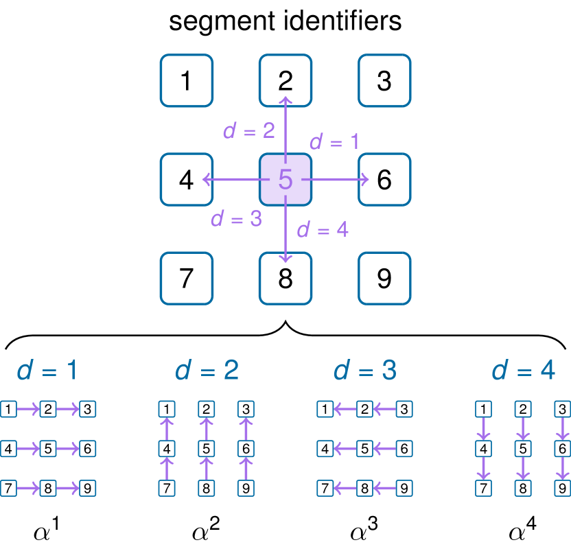
Figure 1: Exemplary nearest neighbor adjacency configuration for CWFC on a two-dimensional grid consisting of $N=9$ segments. The adjacency relationship for each of the four directions right ($d=1$), up ($d=2$), left ($d=3$), and down ($d=4$) can be represented as a directed graph with adjacency matrix $\alpha^{d}$.

Based on the chosen adjacency configuration, a pattern-based value selection can be defined. For this purpose, a more general rule-based selection is introduced first and then the pattern-based selection is presented as a special case.

For a rule-based value selection, consider a set of $m$ rules

$$R:=\{r_{1},\dots,r_{m}\}\in\mathcal{R},$$ (12)

from the set of of all possible rulesets $\mathcal{R}$, where each rule

$$r_{i}:=r_{i}(v,w):=(v,w)$$ (13)

for $i\in[1,m]$ consists of a value $v\in A$ and a weight function $w:=w(i,\alpha^{d},C^{\prime})\in\mathbb{R}_{\geq 0}$ with

$$w:[1,N]\times\mathcal{B}\times\overline{\mathcal{C}}\rightarrow\mathbb{R}_{\geq 0},$$ (14)

where

$$\overline{\mathcal{C}}:=\cup_{k=0}^{N-1}\mathcal{C}(k)$$ (15)

denotes the unified set of all partial contents. Given a ruleset $R\in\mathcal{R}$, the rule-based version of the probability distribution from eq. 6 is defined as

$$p_{k}^{\mathrm{v}}(\nu|i,C^{\prime})=p_{k}^{\mathrm{v,R}}(\nu|i,C^{\prime}):=\frac{F_{k}(\nu,i,C^{\prime})}{\overline{F}_{k}(i,C^{\prime})}$$ (16)

with the abbreviations

$$F_{k}(\nu,i,C^{\prime}):=\sum_{\begin{subarray}{c}(v,w)\in R\\ v=\nu\end{subarray}}w(i,\alpha^{d},C^{\prime})$$ (17)

and

$$\overline{F}_{k}(i,C^{\prime}):=\sum_{\nu\in A}F_{k}(\nu,i,C^{\prime}),$$ (18)

respectively, for $\nu\in A$, $i\in[1,N]$, $C^{\prime}\in\mathcal{C}(k)$ for $k\in[1,N]$, and $\alpha^{d}\in\mathcal{B}$ for $d\in[1,D]$. Summarized, the set of rules $R$ determines how values are selected based on the non-vanishing results of the respective weight functions. Note that condition V1 is always satisfied, whereas in case of $\overline{F}_{k}(i,C^{\prime})\overset{!}{=}0$ for any $C^{\prime}\in\mathcal{C}(k)$ with $p_{k}^{\mathrm{s,H}}(i|C^{\prime})p(C^{\prime})>0$, condition V2 is violated.

Pattern-based value selection is a special case of rule-based value selection, where the weight function

$$w(i,\alpha^{d},C^{\prime})\!:=\!w^{\mathrm{P}}(i,\alpha^{d},C^{\prime},P,u)\!:=\!u\tau(i,\alpha^{d},C^{\prime},P)$$ (19)

of each rule

$$r_{i}:=r_{i}^{\mathrm{P}}(v,P,u):=(v,w^{\mathrm{P}}(i,\alpha^{d},C^{\prime},P,u))$$ (20)

for $i\in[1,m]$ is defined by a non-vanishing factor $u\in\mathbb{R}_{>0}$ and a pattern

$$P:=\{(d_{1},v_{1}),\dots,(d_{n},v_{n})\}\in\mathcal{P}$$ (21)

consisting of a set of $n\leq D$ direction-value pairs with $d_{i}\in[1,D]$ for $i\in[1,n]$, $d_{i}\neq d_{j}\,\forall\,i,j\in[1,n]\land i\neq j$, and $v_{i}\in A$ for $i\in[1,n]$, where

$$\mathcal{P}:=\{P\,|\,P\in([1,D]\times A)^{n}\,\forall\,n\in[0,D]\}$$ (22)

denotes the set of all possible patterns. A pattern $P$ is fulfilled, if

$$\tau(i,\alpha^{d},C^{\prime},P):=\prod_{(d,v)\in P}\prod_{\begin{subarray}{c}(s,v^{\prime})\in C^{\prime}\\ \alpha^{d}_{i,s}=1\end{subarray}}\delta_{vv^{\prime}}\in[0,1]$$ (23)

evaluates to one. Here, $\delta$ represents the Kronecker delta. The set of all possible pattern-based rulesets is denoted by $\mathcal{R}^{\mathrm{P}}\subset\mathcal{R}$.

Summarized, the weight function, eq. 19, yields $u$ if the pattern $P$ applies and zero otherwise. In line with expectations, only adjacent segments (i.e., $\alpha^{d}_{i,s}=1$) have an influence on eq. 16 according to eq. 23.

Furthermore, the rules from eq. 20 can be rewritten as

$$r_{i}^{\mathrm{P}}(v,P,u)=(v,u,P)$$ (24)

for $i\in[1,m]$ with a value $v\in A$, a factor $u\in\mathbb{R}_{>0}$, and a pattern $P\in\mathcal{P}$. For the pattern-based value selection, eq. 16 can be reformulated as

$$p_{k}^{\mathrm{v,R}}(\nu|i,C^{\prime}) =p_{k}^{\mathrm{v,P}}(\nu|i,C^{\prime})$$

$$:=\sum_{\begin{subarray}{c}(v,u,P)\in R\\ v=\nu\end{subarray}}\gamma(u,i,C^{\prime})\tau(i,\alpha^{d},C^{\prime},P)$$ (25)

with the coefficients

$$\gamma(u,i,C^{\prime}):=\frac{u}{\overline{F}_{k}(i,C^{\prime})}\in[0,1]$$ (26)

that correspond to the normalized weights of the rules.

In the context of this manuscript, one variant (that lies between rule- and pattern-based selection) is particularly important, namely the use of a functional factor instead of a constant factor for pattern-based rules of the form of eq. 24. Specifically, a factor

$$u:=u(i,C):[1,N]\times\overline{\mathcal{C}}\rightarrow\mathbb{R}$$ (27)

is considered that can depend both on the coordinate $i\in[1,N]$ and/or the already generated content $C\in\overline{\mathcal{C}}$, eq. 15. By mapping to zero, this functional factor can disable a pattern for certain coordinates or partial contents.

1.2.2 Identifier selection.

For the entropic segment identifier selection, the probability distribution from eq. 5 is defined as

$$p_{k}^{\mathrm{s}}(i|C^{\prime})=p_{k}^{\mathrm{s,H}}(i|C^{\prime}):=\begin{cases}|I_{k}(C^{\prime})|^{-1}&\text{if }i\in I_{k}(C^{\prime})\\ 0&\text{otherwise}\end{cases}$$ (28)

with the set of optimal solutions

$$I_{k}(C^{\prime}):=\{i\,|\,i\in S^{-}(C^{\prime})\land H_{k}(i,C^{\prime})=h_{k}(C^{\prime})\}$$ (29)

of the optimization task

$$h_{k}(C^{\prime}):=\operatorname*{arg\,min}_{j\in S^{-}(C^{\prime})}H_{k}(j,C^{\prime}),$$ (30)

where

$$H_{k}(i,C^{\prime}):=-\sum_{v\in A} p_{k}^{\mathrm{v,P}}(\nu=v|i,C^{\prime})$$

$$\times\ln p_{k}^{\mathrm{v,P}}(\nu=v|i,C^{\prime})$$ (31)

denotes the Shannon information entropy for $C^{\prime}\in\mathcal{C}(k-1)$, $k\in[1,N]$ . That is, the segments with the smallest Shannon entropy with respect to the available value options are chosen.

1.3 CWFC Example: Checkerboard

As a simple example, consider the generation of images with black and white checkerboard patterns. The pixels of an image constitute the segments and the alphabet consists of only $W=2$ symbols standing for the two colors. As an adjacency configuration, the nearest-neighbor adjacency from fig. 1 is presumed.

A checkerboard image can be achieved with only two patterns of the form of eq. 21, namely $P_{1}:=\{(1,1),(2,1),(3,1),(4,1)\}$ and $P_{2}:=\{(1,2),(2,2),(3,2),(4,2)\}$. The corresponding ruleset, eq. 12, reads $R=\{r_{1}^{\mathrm{P}},r_{2}^{\mathrm{P}}\}$ and therefore contains the $m=2$ rules $r_{1}^{\mathrm{P}}(v=2,P=P_{1},u=1)$ and $r_{2}^{\mathrm{P}}(v=1,P=P_{1},u=1)$ based on eq. 20, see fig. 2.

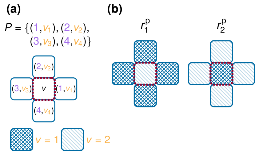
Figure 2: Visualization of pattern-based rules. (a) Visualization scheme. The center tile corresponds to the target segment $i$ of the weight function, eq. 19, with a target value of $v$, whereas the adjacent tiles represent the required values $v_{1},\dots,v_{4}\in\{1,2\}$ of the four adjacent segments in the respective directions $d=1,\dots,d=4$. (b) Pattern-based rules $r_{1}^{\mathrm{P}}(v=2,P=P_{1},u=1)$ and $r_{2}^{\mathrm{P}}(v=1,P=P_{2},u=1)$, eq. 20, that can be used for the generation of images with black and white checkerboard patterns.

The iterative process of CWFC is sketched in fig. 3 for a $3\times 3$ image (represented by $N=9$ segments). Only two content instances can be generated, $C_{1}:=\{(1,1),\dots\}$ and $C_{2}:=\{(1,2),\dots\}$ with equal probability, eq. 10. The choice of the first value $v_{s(1)}$ already determines the choices of all other values.

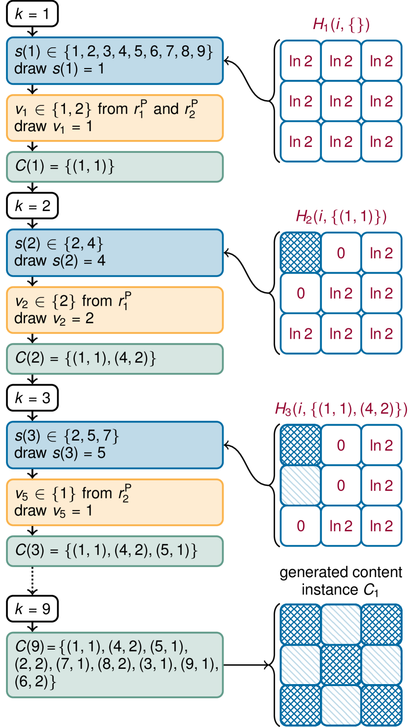
Figure 3: CWFC for the generation of $3\times 3$ images with checkerboard patterns defined by the rules from fig. 2. In each iteration $k\in[1,9]$, three steps take place: (i) a segment identifier $s(k)$ is drawn, eq. 28, (ii) a corresponding value $v_{s(k)}$ is drawn, section 1.2.1, and (iii) the newly generated identifier-value pair is added as a segment to the content instance $C(k)$. For $s(k)$ and $v(k)$, the uniformly distributed set of possible choices are listed. The choices for $s(k)$ depend on the Shannon entropy $H_{k}$, section 1.2.2, of each undefined segment, as shown on the right. The choices for $v(k)$ depend on the fulfillment of the two rules $r_{1}^{\mathrm{P}}$ and $r_{2}^{\mathrm{P}}$, as listed.

2 QUANTUM METHODS

Based on the previously established classical concepts, a QWFC method and a HWFC method are proposed in the following. A software implementation is available online [9].

2.1 Quantum Wave Function Collapse (QWFC)

So far, the procedural generation concepts have been presented from a purely classical perspective. However, it seems natural that the probability distribution of the content instances $p(C)$, eq. 10, can also be realized with the help of a quantum circuit by utilizing the intrinsic randomness of quantum physics [10]. This is the very idea on which QWFC is based.

A single alphabet $A$ with $W$ symbols is presumed, eq. 11. Furthermore, two procedures control the content generation, namely segment identifier selection and value selection.

2.1.1 Identifier selection.

The Identifier selection is performed with a predefined order given by the vector $\sigma\in S_{N}$, which is the set of all permutations of $[1,N]$. Hence,

$$p_{k}^{\mathrm{s}}(i|C^{\prime})=p_{k}^{\mathrm{s,o}}(i|C^{\prime}):=\delta_{i\sigma_{i}}.$$ (32)

This approach leads to (partial) content instances $\mathcal{C}(k)=\mathcal{C}_{\sigma}(k)$, eq. 2, of the form

$$\mathcal{C}_{\sigma}(k):=\{C\,|\, C=\{(\sigma_{1},v_{\sigma_{1}}),\dots,(\sigma_{k},v_{\sigma_{k}})\}$$

$$\,\forall\,v_{\sigma_{l}}\in A\,\forall\,l\in[1,k]\}$$ (33)

for $k\in[1,N]$ and $\mathcal{C}_{\sigma}(0):=\{\{\}\}$.

2.1.2 Value selection.

The value selection is pattern-based in analogy to section 1.2.1. In particular, the value for each segment is encoded by a set of qubits, which requires

$$q:=\lceil\log_{2}W\rceil$$ (34)

qubits for each segment $i\in[1,N]$. The group of $q$ qubits that represent the value for segment $i$ is denoted by

$$\mathcal{Q}_{i}:=\{q_{i}^{1},\dots,q_{i}^{q}\},$$ (35)

where $q_{i}^{j}$ references the $j$th qubit of this group for $j\in[1,q]$. The state of these qubits encodes the value $v_{i}$ of the segment $i$ in binary as the tensor product sequence of qubit states

$$\bigotimes_{j=1}^{q}\ket{b_{j}}=\Ket{v_{i}-1=\sum_{j=1}^{q}b_{j}2^{j-1}}_{i}=\ket{v_{i}-1}_{i}\in\mathcal{H}_{i}$$ (36)

with $b_{j}\in\mathbb{B}$, $v_{i}\in A$, and $i\in[1,N]$, where $\mathcal{H}_{i}$ denotes the joint Hilbert space of all qubit from $\mathcal{Q}_{i}$.

In total,

$$Q:=Nq$$ (37)

qubits are required to represent the value of all $N$ segments. The joint Hilbert space of all qubits from $\bigcup_{i=1}^{N}\mathcal{Q}_{i}$ is given by $\mathcal{H}:=\bigotimes_{i=1}^{N}\mathcal{H}_{i}$ and a state $\ket{\Psi}\in\mathcal{H}$ can realize samples from a specific probability distribution of content instances

$$p(C\!=\!\{(1,v_{1}),\dots,(N,v_{N})\})=|\bra{\Psi}\bigotimes_{i=1}^{N}\ket{v_{i}-1}_{i}|^{2}.$$ (38)

based on a projective measurement. After these preliminary considerations, the remaining question is how such a state can be prepared constructively with quantum gates from a given pattern-based ruleset. This question will be answered in the following.

2.1.3 Quantum circuit.

Initially, all qubits are prepared in the ground state, i.e., $\ket{\Psi}=\ket{0}:=\bigotimes_{i=1}^{N}\ket{0}_{i}$. Then, given a pattern-based ruleset $R\in\mathcal{R}^{\mathrm{P}}$, eq. 12, a series of operators is applied, one for each iteration $k\in[1,N]$ such that $\ket{\Psi}:=U_{N}\cdots U_{1}\ket{0}$ represents the final state after $k$ iterations. In each iteration $k$, the state of the qubits $\mathcal{Q}_{\sigma_{k}}$ (that represent the value for segment $\sigma_{k}$) is prepared conditioned on the state of (a subset of) the qubits $\mathcal{Q}_{\sigma_{1}},\dots,\mathcal{Q}_{\sigma_{k-1}}$ (that represent the values of the already prepared segments $\sigma_{1},\dots,\sigma_{k-1}$), which leads to an entangled joint state. A sketch is shown in fig. 4 (a).

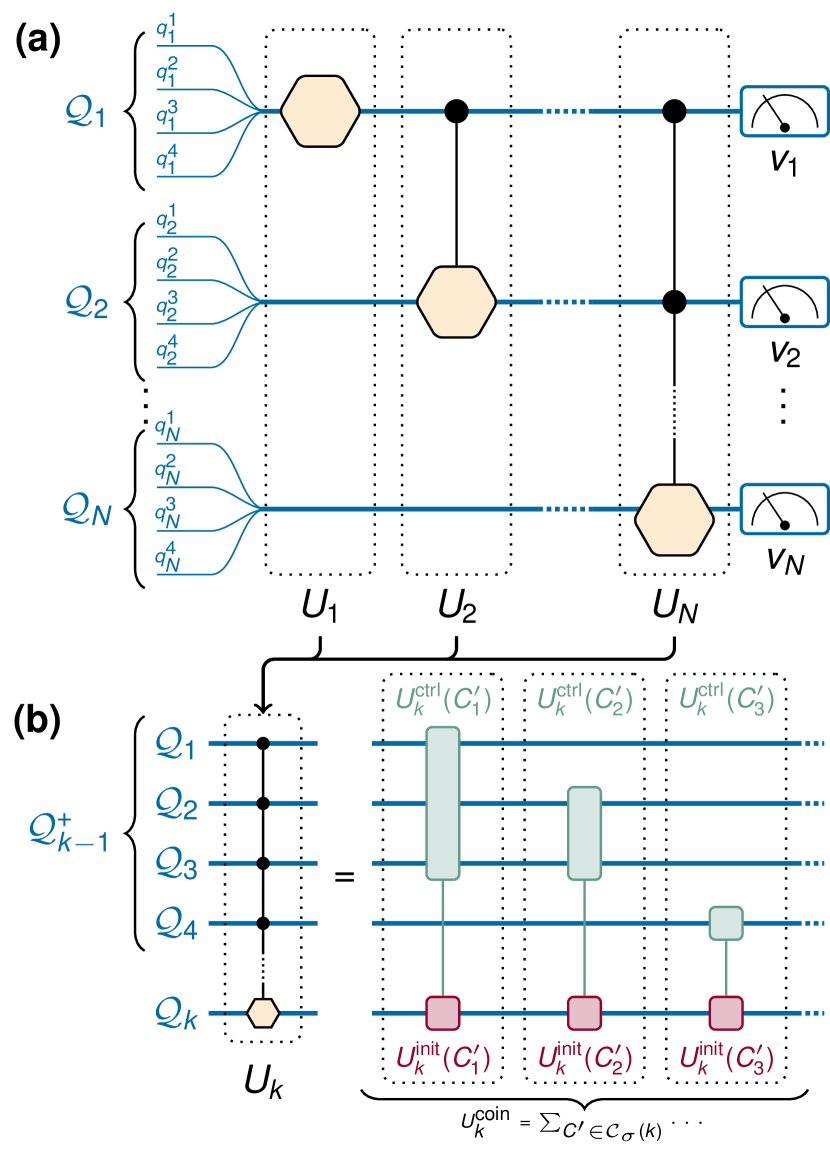
Figure 4: QWFC circuit with $\sigma=(1,\dots,N)$. (a) Circuit layout with an exemplarily alphabet $A$, eq. 11, with $W=16$ symbols, which requires a set $\mathcal{Q}_{i}$, eq. 35, of $q=4$ qubits, eq. 34, for each segment with $i\in[1,N]$. In each iteration $k\in[1,N]$, the operator $U_{k}$, eq. 39, prepares the qubits from $\mathcal{Q}_{k}$ in a superposition state $\ket{C^{\prime}}_{k}$, eq. 43, entangled with (a subset of) the qubits from $\mathcal{Q}_{1},\dots,\mathcal{Q}_{k-1}$. All qubits are measured to obtain $p(C)$, eq. 38. (b) Gate decomposition of $U_{k}$ into the components of $U_{k}^{\mathrm{coin}}$, eq. 40, which consists of pairs $U_{k}^{\mathrm{ctrl}}(C^{\prime})\otimes U_{k}^{\mathrm{init}}(C^{\prime})$, eqs. 41 and 42. Each of these pairs represent a conditional loading of a probability distribution to realize $\ket{C^{\prime}}_{k}$ (which is not explicitly shown). The combined control operators act on the qubits from $\mathcal{Q}_{k}^{+}$ eq. 45, whereas the initialization operators act on the qubits from $\mathcal{Q}_{k}$.

Specifically,

$$U_{k}:=\left[U_{k}^{\mathrm{coin}}+U_{k}^{0}\right]\otimes\bigotimes_{l=k+1}^{N}\mathbbm{1}_{\sigma_{l}}\in\mathcal{H}$$ (39)

for $k\in[1,N]$ contains $\mathbbm{1}_{i}\in\mathcal{H}_{i}$, the unit operator for $i\in[1,N]$ and two other operators. First, the conditional initialization operator

$$U_{k}^{\mathrm{coin}}=\sum_{C^{\prime}\in\mathcal{C}_{\sigma}(k)}\left[U_{k}^{\mathrm{ctrl}}(C^{\prime})\otimes U_{k}^{\mathrm{init}}(C^{\prime})\right],$$ (40)

where $\mathcal{C}_{\sigma}(k)$ represents the set of possible partial content instances from section 2.1.1,

$$U_{k}^{\mathrm{ctrl}}(C^{\prime}):=\bigotimes_{(s,v)\in L_{k}(C^{\prime})}\ket{v-1}\bra{v-1}_{s}\in\bigotimes_{l=1}^{k-1}\mathcal{H}_{\sigma_{l}}$$ (41)

denotes the control operator, and

$$U_{k}^{\mathrm{init}}(C^{\prime}):=\ket{C^{\prime}}\bra{0}_{\sigma_{k}}\in\mathcal{H}_{\sigma_{k}}$$ (42)

the initialization operator with

$$\ket{C^{\prime}}_{\sigma_{k}}:=\sum_{\nu\in A}\sqrt{p_{k}^{\mathrm{v,P}}(\nu|\sigma_{k},C^{\prime})}\ket{\nu-1}_{\sigma_{k}}\in\mathcal{H}_{\sigma_{k}},$$ (43)

which is based on the pattern-based probability distribution of values $p_{k}^{\mathrm{v,P}}(\nu|i,C^{\prime})$ from section 1.2.1. The summation in eq. 41 runs over all adjacent segments

$$L_{k}(C^{\prime}):=\{(s,v)\,|\, (s,v)\in C^{\prime}\,\land\,\exists\,P\in R_{P}$$

$$\exists\,d\in P_{d}:\alpha^{d}_{\sigma_{k}s}=1\}\subseteq C^{\prime},$$ (44)

where $R_{P}:=\{P_{1},\dots,P_{m}\}$ stands for the set of patterns in the pattern-based ruleset $R\in\mathcal{R}^{\mathrm{P}}$ with $P_{i}\in\mathcal{P}$ for $i\in[1,m]$ and $P_{d}:=\{d_{1},\dots,d_{n}\}$ stands for the set of directions in the pattern $P\in\mathcal{P}$, eq. 21, with $d_{j}\in[1,D]$ for $j\in[1,n]$. In particular, as discussed above for the classic case, choosing $C^{\prime}$ instead of $L_{k}(C^{\prime})$ in the summation has no effect on $p_{k}^{\mathrm{v,P}}(\nu|i,C^{\prime})$ and thus $\ket{C^{\prime}}_{\sigma_{k}}$.

In iteration $k$, only the qubits in $\mathcal{Q}_{k-1}^{+}$ with

$$\mathcal{Q}_{k}^{+}:=\{q\,|\,q=q_{k}^{i}\in\mathcal{Q}_{\sigma_{k}}\,\forall\,i\in[1,q]\,\land\,\sigma_{k}\in L_{k}^{+}\}$$ (45)

are affected by $U^{\mathrm{ctrl}}(C^{\prime})$ for some $C^{\prime}\in\mathcal{C}_{\sigma}(k)$, where

$$L_{k}^{+}:=\{s\,|\,\exists\,C^{\prime}\in\mathcal{C}_{\sigma}(k)\,:\,s\in S^{+}(L_{k}(C^{\prime}))\}$$ (46)

denotes the affected segments for $k=[1,N]$. Here, $\mathcal{Q}_{k}^{+}\subseteq\{\mathcal{Q}_{1},\dots,\mathcal{Q}_{k}\}$ and $L_{k}^{+}\subseteq\{\sigma_{1},\dots,\sigma_{k}\}$, respectively.

The second operator in eq. 39 is the neutral operator

$$U_{k}^{0}=\sum_{C^{\prime}\in\mathcal{C}_{\sigma}(k)}\left[U_{k}^{\mathrm{ctrl}}(C^{\prime})\otimes U_{k}^{\mathrm{init},0}+U_{k}^{\mathrm{ctrl},0}(C^{\prime})\right].$$ (47)

Initially, all qubits $\mathcal{Q}_{k}$ are in the ground state. Therefore,

$$U_{k}^{\mathrm{init},0}:=\sum_{v\in[2,W]}\ket{v-1}\bra{v-1}_{\sigma_{k}}\in\mathcal{H}_{\sigma_{k}}$$ (48)

vanishes. Furthermore,

$$U_{k}^{\mathrm{ctrl},0}(C^{\prime})\!:=\!\left[\bigotimes_{l=1}^{k-1}\mathbbm{1}_{\sigma_{l}}-U_{k}^{\mathrm{ctrl}}(C^{\prime})\right]\otimes\mathbbm{1}_{\sigma_{k}}\!\in\bigotimes_{l=1}^{k}\mathcal{H}_{\sigma_{l}}$$ (49)

does not change the state by construction.

The operator $U_{k}$, eq. 39, can be straightforwardly realized with quantum gates for a given $k\in[1,N]$. To this end, only the conditional initialization operator $U_{k}^{\mathrm{coin}}$, eq. 40, has to be considered because all other parts of $U_{k}$ have no effect on the resulting state. The conditional initialization operator consist of a sequence of joint pairs of control-initialization operators $U_{k}^{\mathrm{ctrl}}(C^{\prime})\otimes U_{k}^{\mathrm{init}}(C^{\prime})$, one for each $C^{\prime}\in\mathcal{C}_{\sigma}(k)$. Each of these joint pairs represent a conditional loading of a probability distribution to realize $\ket{C^{\prime}}_{\sigma_{k}}$, which is a well-known task that may, however, require an exponential number of gates [11, 12, 13]. A sketch is shown in fig. 4 (b).

For the definition of QWFC, a noise-free, ideal quantum device is presumed, that is able to run the emerging circuits without any errors. However, the currently available noisy intermediate-scale quantum (NISQ) hardware exhibits significant noise and uncertainty [14]. As a consequence, the content sampled from eq. 38 can also be expected to violate the prescribed patterns. This will be demonstrated further below for several PCG use cases.

The proposed conditions S1, S2, V1, and V2 are in fact not mandatory in the original implementation of CWFC, where a violation leads to a restart of the algorithm. This can also be considered in QWFC by adding an additional “conflict detection qubit” that stores this information, an extension that is not further discussed here.

2.2 QWFC Example: Checkerboard

In the following, the above example for the generation of $3\times 3$ checkerboard images is considered for QWFC, where the predefined segment order $\sigma=(1,2,3,6,5,4,7,8,9)$ is used for eq. 32 as visualized in fig. 5 (a). The resulting CWFC circuit is shown in fig. 5 (b) and the resulting probability distribution of content instances $p(C)$, eq. 38, in fig. 5 (c). Given a noise-free quantum device, a measurement of the circuit corresponds to drawing a sample from this distribution.

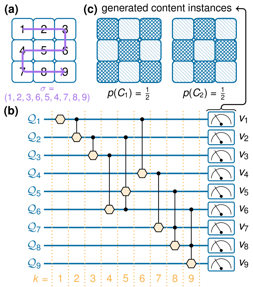
Figure 5: QWFC for the generation of $3\times 3$ images with black and white checkerboard patterns in analogy to fig. 3. (a) Predefined segment order $\sigma=(1,2,3,6,5,4,7,8,9)$ for eq. 32. (b) Circuit layout with the same symbols as in fig. 4. (c) Generated content instances $C_{1}$ and $C_{2}$ with $p(C_{1})=p(C_{2})=\frac{1}{2}$, eq. 38.

2.3 Hybrid Quantum-Classical WFC (HWFC)

The required number of qubits for the proposed QWFC method increases linearly with the number of segments and logarithmically with the number of symbols in the alphabet as shown in eqs. 34 and 37. At the same time, the respective circuits may become exponentially deeper because of the costly conditional preparation of probability distributions. The reliable execution of such big circuits on NISQ hardware can be very challenging or even impossible.

As an alternative, a quantum-classical hybrid approach called HWFC is proposed in the following. To realize this approach, the content has to be separated into $H$ partitions, each of which contains a subset of the segments. That is, partition $h\in[1,H]$ contains all of the segment identifiers from the set $S^{h}\subset[1,N]$ with $\bigcup_{h=1}^{H}S^{h}=[1,N]$ and $\bigcap_{h=1}^{H}S^{h}=\{\}$. For each partition $h\in[1,H]$, a QWFC is performed, which yields the content instance partition $C^{h}$ as a sample of the random variable $\boldsymbol{C}^{h}\sim p(C^{h}):=p^{h}(C^{h}|C^{1},\dots,C^{h-1})$ in analogy to eq. 38. For the QWFC on the partition, two modifications are required. First, the iteration over all segment identifiers $[1,N]$ is replaced by the iteration over the segment identifiers from $S^{h}$. Second, the already sampled sub-contents $C^{1},\dots,C^{h-1}$ from the partitions $[1,h-1]$ are used as an additional constraint for the pattern-based rules. That is, $\mathcal{C}_{\sigma}(k)$ in eqs. 40 and 47 is replaced by $\mathcal{C}^{h}_{\sigma}(k):=\{C\,|\,C=\bigcup_{i=1}^{h-1}C^{i}\cup C^{\prime}\,\forall\,C^{\prime}\in\mathcal{C}_{\sigma}(k)\}$ for $h\in[1,H]$. This modification induces classical correlations from previously sampled content partitions into the circuit, which is why the phrasing conditional QWFC is used for the modified QWFC on the partition.

Finally, the distribution of the joint content instances is given by

$$p\left(C=\bigcup_{h=1}^{H}C^{h}\right)=\prod_{h=1}^{H}p^{h}(C^{h}|C^{1},\dots,C^{h-1}),$$ (50)

which corresponds to performing a QWFC on the complete content, cf. fig. 6. With the proposed HWFC method, the size of the QWFC circuits can be reduced at the price of an additional outer iteration loop and the inclusion of classical correlations in the conditional QWFC circuit generation.

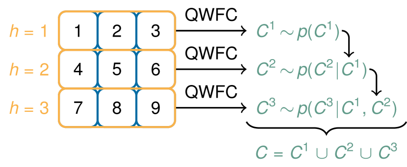
Figure 6: HWFC with $H=3$ partitions of $N=9$ segments. For each partition, a conditional QWFC is performed and the resulting content instances are combined.

3 DEMONSTRATION

In the present section, five simple content creation use cases are presented to demonstrate the proposed QWFC and HWFC methods. For the realization of these examples, both quantum computing simulators and actual IBM Quantum devices were used, which were accessed via the IBM Quantum cloud services [15] during December 2023.

3.1 Checkerboard Revisited

As a first use case, the previously presented checkerboard example is recalled, cf. figs. 2 and 5. Again, $3\times 3$ instances are considered, for which a comparison between QWFC and HWFC is performed on the IBM Quantum device ibm_kyoto (Eagle r3 processor version 1.2.4, 127 qubits). For QWFC, $10\,000$ shots are measured, each yielding a content instance. For HWFC, $H=3$ equal-sized partitions are used in analogy to fig. 6 and the method is repeated $131$ times, each time yielding a content instance. The results are shown in fig. 7.

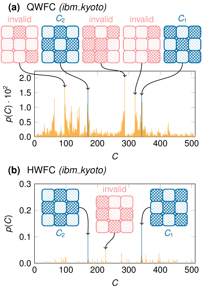
Figure 7: Checkerboard generation. Plots show the generated content instances $C$, eq. 1, (encoded as integers in $[0,511]$ from the measured bit strings) and their respective probabilities $p(C)$, eq. 38. (a) QWFC on the IBM Quantum device ibm_kyoto. The inset plot shows the dominating instances ($p(C)>$1.4\text{\times}{10}^{-2}$$). (b) HWFC with $H=3$ on the same device results in less invalid instances.

In total, there are $2^{9}=512$ possible content instances $C\in\mathcal{C}$, eq. 1, but only two of them, $C_{1}$ and $C_{2}$, are valid. The remaining $510$ content instances are invalid because they violate the patterns. In fig. 7 (a), QWFC is able to generate the two valid instances, but at the same time also produces a lot of invalid instances due to hardware imperfections. From fig. 7 (b) it can be seen that the results from HWFC are much closer to the idealized solution that would contain only $C_{1}$ and $C_{2}$ with equal probability. It is a consequence of the reduced circuit size from this method that invalid solutions occur with much less frequency than for QWFC.

3.2 Pipes

The second use case is to create an image from tiles of seven different pipe (or line) sections as well as one blank tile. That is, the alphabet consists of $W=8$ symbols and each tile in the image constitutes a segment. The alphabet is shown in fig. 8 (a). As adjacency configuration, the nearest-neighbor adjacency from fig. 1 is presumed with $D=4$. The pattern-based ruleset is chosen in such a way that neighboring tiles have to form a connecting network of pipes. Three example rules for this purpose are shown in fig. 8 (b). In total, $m=2048$ rules are required to achieve this goal.

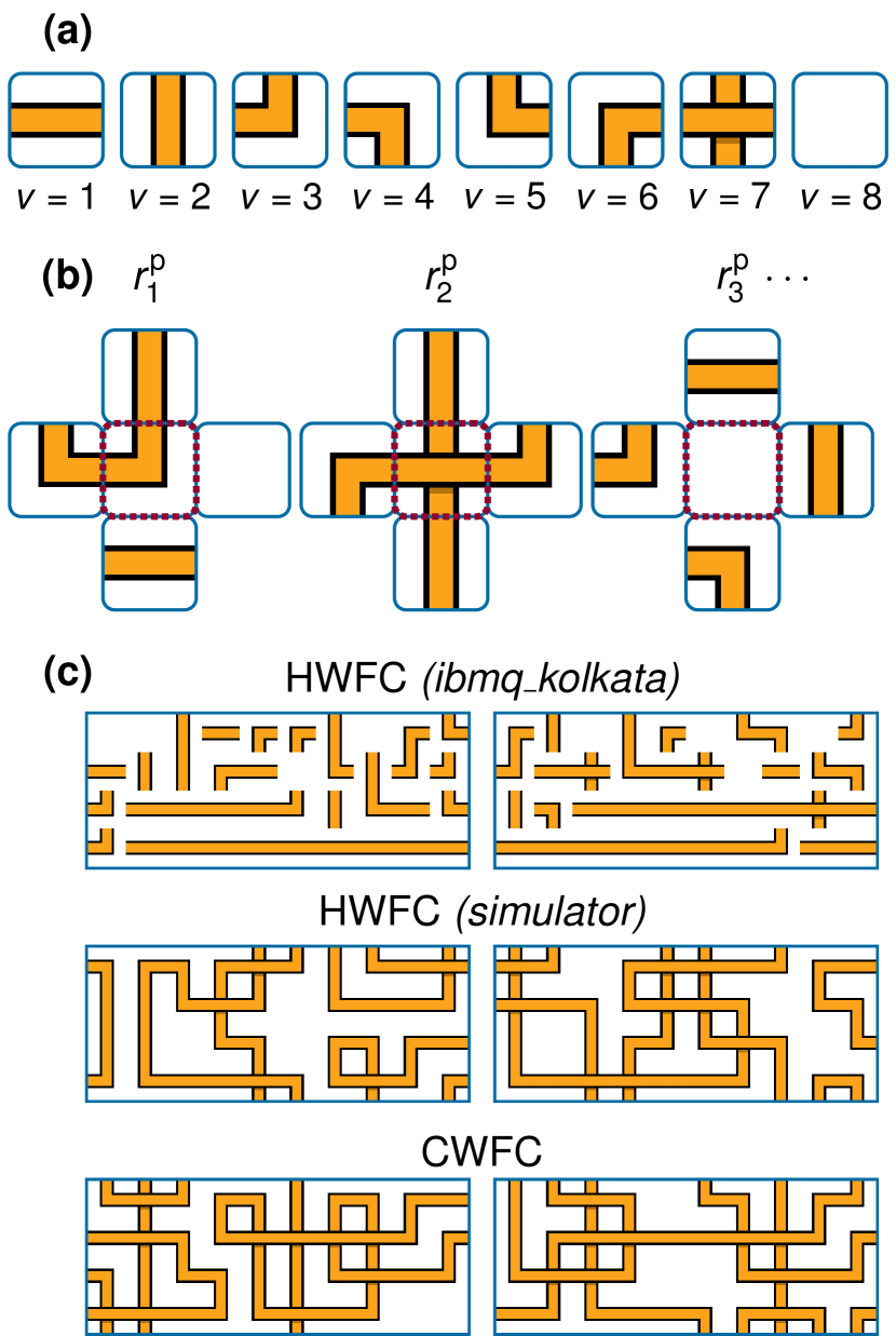
Figure 8: Pipe generation. The generated image is required to show a network of connected pipes. (a) Alphabet consisting of $W=8$ symbols, each of which represents a tile with a pipe section and an empty tile. (b) Example of three pattern-based rules $r_{1}^{\mathrm{p}}$, $r_{2}^{\mathrm{p}}$, and $r_{3}^{\mathrm{p}}$, cf. fig. 2. (c) Example $10\times 4$ tile images that were generated using HWFC with $H=10$ on the IBM Quantum device ibm_kolkata and on simulator as well as CWFC.

Exemplarily, images consisting of $10\times 4$ tiles ($N=40$) are considered, for which a comparison between HWFC on the IBM Quantum device ibm_kolkata (Falcon r5.11 processor version 1.14.8, 27 qubits), HWFC on a simulator and CWFC is performed. For HWFC, $H=10$ equal-sized partitions are used, each corresponding to one column of the image. A few resulting instances are shown in fig. 8 (c).

Based on a visual comparison, both CWFC and HWFC on the simulator yield similar results, as expected. However, the results from ibm_kolkata clearly contain a lot of invalid patterns as a result of the imperfect hardware. This demonstrates the limitations of the proposed method on NISQ devices.

3.3 Hexagon Map

The third use case addresses images based on hexagonal tiles that can be interpreted as a map consisting of different terrains. For this purpose, an alphabet of $W=4$ symbols is chosen, each corresponding to a unicolored tile (blue, yellow, green, and gray) and each tile constitutes a segment. As adjacency configuration, a nearest-neighbor adjacency is presumed ($D=6$). The prescribed pattern-based ruleset only allows connections of the form blue-yellow-green-gray, which can be fulfilled with $m=1586$ rules, see fig. 9 (a). To promote a higher occurrence of blue tiles, the factors in eq. 24 are chosen as $u=5$ for blue tiles and $u=1$ otherwise.

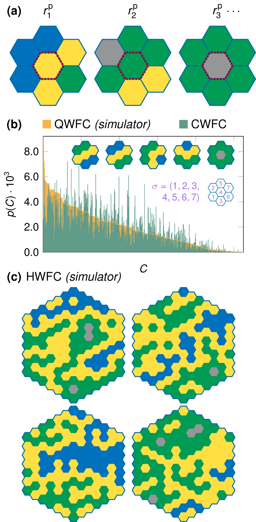
Figure 9: Map generation. Only connections of the form blue-yellow-green-gray are allowed. (a) Example of three pattern-based rules $r_{1}^{\mathrm{p}}$, $r_{2}^{\mathrm{p}}$, and $r_{3}^{\mathrm{p}}$. (b) Distribution of content instances $p(C)$ for $N=7$ hexagons using QWFC on a simulator (sorted by descending probability) and CWFC (with the same ordering). The inset plot shows the predefined segment order $\sigma$ and the five most probable instances for QWFC. The asymmetry is a consequence of the choice of $\sigma$. (c) Example images that were generated from $N=127$ hexagons using HWFC with $H=20$ on a simulator.

As a first example, images consisting of $N=7$ tiles are considered, for which QWFC on a simulator and CWFC are performed. The resulting distributions of content instances $p(C)$ in fig. 9 (b) is exact for QWFC, eq. 38, and based on $10\,000$ samples for CWFC, eq. 10. Without surprise, both distributions are significantly different. The second example considers images from $N=127$ tiles, for which HWFC with $H=20$ is performed on a simulator. Example instances are shown in fig. 9 (c).

3.4 Platformer

The fourth use case is motivated by computer game level design. The goal is to create a platformer-type level from a set of eight tiles [16], each corresponding to a different game element (ground, grass, mushroom, block, air, and a tree that is composed of three tiles). Consequently, the alphabet consists of $W=8$ symbols, see fig. 10 (a). As adjacency configuration, the two tiles above and below are taken into account as neighbors ($D=2$). A pattern-based ruleset is prescribed that meets five requirements: (i) The bottom row consists of ground tiles and ground tiles can only be placed on top of each other, (ii) only a grass tile or a mushroom tile can be placed above a ground tile, (iii) the tree tiles must be placed in order with the lowest tile above a grass tile, (iv) air tiles can only be placed above grass, mushroom or other air tiles, (v) block tiles can only be placed between two air tiles. These requirements can be fulfilled with $m=15$ rules, see fig. 10 (b). The first requirement can be resolved with a functional factor, eq. 27, that vanishes for all non-ground tiles in the bottom row. To reduce the occurrence of block tiles, the corresponding factor in eq. 24 is chosen as $u=$0.1$$ for $r_{6}^{\mathrm{p}}$. All other factors are set to $u=1$. The segment order $\sigma$ is chosen such that the levels are built up from bottom to top.

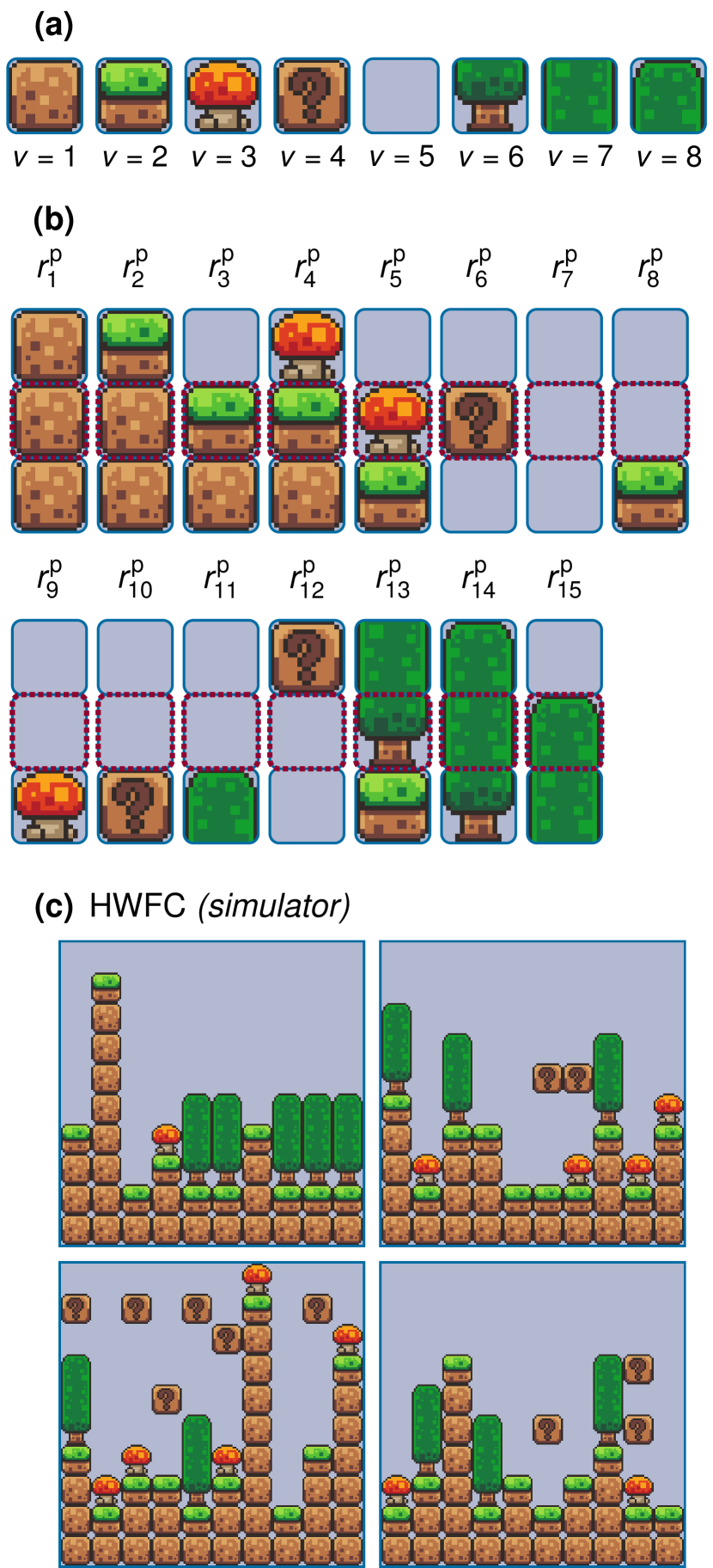
Figure 10: Level generation. (a) Alphabet consisting of eight symbols, each of which represents a tile [16]. (b) Pattern-based ruleset consisting of $m=15$ rules. (c) Example $10\times 10$ tile images that were generated using HWFC with $H=20$ on a simulator.

Exemplarily, levels with $10\times 10$ tiles are considered, for which HWFC with $H=20$ equal-sized partitions (each corresponding to a half row of the level) is performed on a simulator. Four resulting instances are shown in fig. 10 (c).

3.5 Voxel Skyline

The final use case considers the creation of a 3d voxel graphic with a binary alphabet of $W=2$ symbols, which represent the presence or absence of a voxel. Each voxel constitutes a segment, as adjacency configuration the voxel above and below are taken into account ($D=2$). The chosen pattern-based ruleset with $m=4$ ensures that voxels are built from the ground up, see fig. 11 (a). This leads to a skyline-like structure.

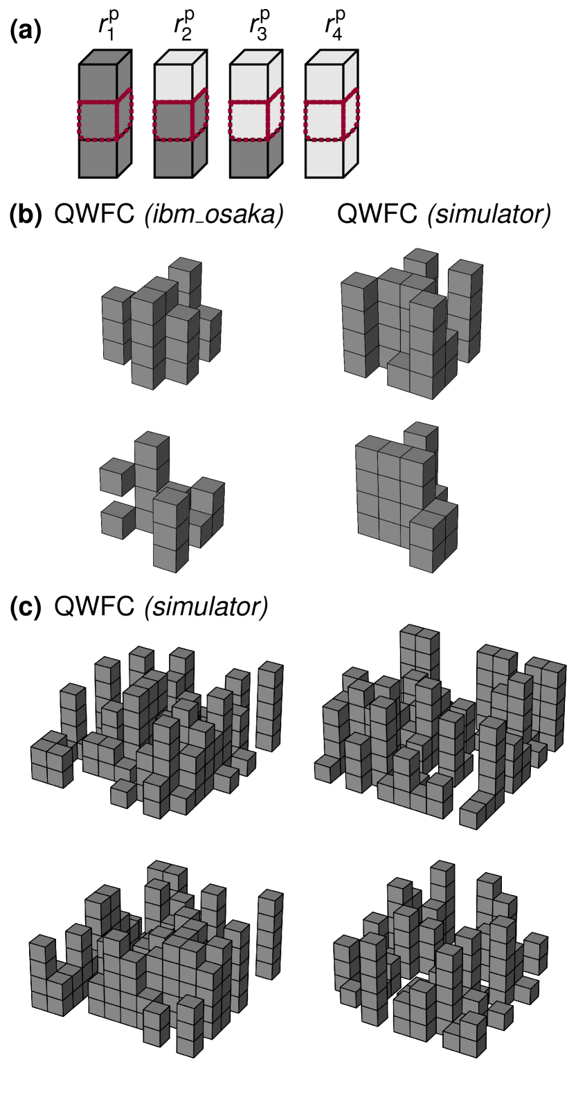
Figure 11: Skyline use case. (a) Pattern-based ruleset consisting of $m=4$ rules in an analogous representation as in the previous figures. (b) Example images from a $4\times 4\times 4$ voxel grid that were generated using QWFC on the IBM Quantum device ibm_osaka and a simulator. (c) Example images from a $10\times 10\times 5$ voxel grid that were generated using QWFC on a simulator.

Exemplarily, two cases are considered: First, images from a $4\times 4\times 4$ voxel grid, for which QWFC is performed both on a the IBM Quantum device ibm_osaka (Eagle r3 processor version 1.0.3, 127 qubits) and a simulator, see fig. 11 (b). An error violating $r_{3}^{\mathrm{p}}$ can be seen in the bottom left image that results from hardware imperfections. Second, images from a $10\times 10\times 5$ voxel grid, for which QWFC is performed on a simulator, see fig. 11 (c).

4 CONCLUSIONS

In this work, QWFC was proposed as a method to realize WFC on a quantum computer for PCG. The idea is to construct a quantum circuit from which valid content instance (that fulfill the prescribed patterns) can be sampled via measurements. In other words, the quantum circuit acts as a special-purpose random generator for content of a desired form that makes use of the intrinsic randomness of quantum physics. This method is not without its challenges. The corresponding quantum circuit becomes larger from both the content and alphabet size and at the same time deeper from the correlations within the content instance distribution, which makes it difficult to evaluate most use cases on current hardware. For this reason, the quantum-classical hybrid method HWFC was proposed that decomposes the problem into smaller sub-problems which can then be executed on the quantum computer with a higher chance of success.

The experimental results have shown the limitations of QWFC and HWFC, but have also proven that at least simple examples can already be implemented on today’s quantum hardware. Furthermore, all experiments were carried out without quantum error correction [17], which can be used to possibly improve the results. The biggest bottleneck of the circuit complexity is the conditional preparation of probability distributions. Investigating possible improvements in this area with regard to specific PCG use cases or alternative preparation approaches (e.g., qGANs [18]) could therefore be a potential direction for future research.

The conceptual advantage of QWFC is that a circuit, once prepared, represents the distribution of content instances. This means that new instances can be generated by simple measurements without any additional algorithmic effort. A shortcoming of QWFC is that only a fixed order of segments is considered instead of a dynamic (e.g., entropy-based) order that depends on the previously selected segments. The realization of such a generalization of the method could also be a point of origin for further studies.

CWFC is a strong method with many areas of application. In this paper, only visual content creation use cases were presented, but QWFC can also be used for non-visual contents like text [9] in analogy to CWFC [19].

In conclusion, the paper aims to provide an initial approach to QWFC that demonstrates its feasibility but leaves room for improvement and raises the question of useful application areas given the limits of NISQ devices.

5 ACKNOWLEDGMENTS

Parts of this research have been funded by the Ministry of Science and Health of the State of Rhineland-Palatinate (Germany) as part of the project AnQuC.

References

- [1] Maxim Gumin. WaveFunctionCollapse. https://github.com/mxgmn/WaveFunctionCollapse, 2016.
- [2] Isaac Karth and Adam M. Smith. Wave function collapse is constraint solving in the wild. In Proceedings of the 12th International Conference on the Foundations of Digital Games, FDG ’17, New York, NY, USA, 2017. Association for Computing Machinery.
- [3] Isaac Karth and Adam M. Smith. Wavefunctioncollapse: Content generation via constraint solving and machine learning. IEEE Transactions on Games, 14(3):364–376, 2022.
- [4] Yuhe Nie, Shaoming Zheng, Zhan Zhuang, and Xuan Song. Extend wave function collapse to large-scale content generation, 2023.
- [5] James R. Wootton. Procedural generation using quantum computation. In International Conference on the Foundations of Digital Games, FDG’20. ACM, September 2020.
- [6] James Wootton and Marcel Pfaffhauser. Investigating the usefulness of quantum blur. 2023.
- [7] James R. Wootton. A quantum procedure for map generation. In 2020 IEEE Conference on Games (CoG). IEEE, 8 2020.
- [8] Laura J. Piispanen. Designing quantum games and quantum art for exploring quantum physics. In 2023 IEEE Conference on Games (CoG), pages 1–8, 2023.
- [9] Raoul Heese. Quantum Wave Function Collapse. https://github.com/RaoulHeese/QWFC, 2023.
- [10] Johannes Kofler and Anton Zeilinger. Quantum information and randomness. European Review, 18(4):469–480, 2010.
- [11] Lov Grover and Terry Rudolph. Creating superpositions that correspond to efficiently integrable probability distributions, 2002.
- [12] Martin Plesch and Časlav Brukner. Quantum-state preparation with universal gate decompositions. Physical Review A, 83(3), 3 2011.
- [13] Kalyan Dasgupta and Binoy Paine. Loading probability distributions in a quantum circuit, 2022.
- [14] John Preskill. Quantum Computing in the NISQ era and beyond. Quantum, 2:79, August 2018.
- [15] IBM. IBM Quantum. https://quantum.ibm.com, 2021.
- [16] RottingPixels. 2D Four Seasons Platformer Tileset [16x16]. https://opengameart.org/content/2d-four-seasons-platformer-tileset-16x16, 2019.
- [17] Zhenyu Cai, Ryan Babbush, Simon C. Benjamin, Suguru Endo, William J. Huggins, Ying Li, Jarrod R. McClean, and Thomas E. O’Brien. Quantum error mitigation. Rev. Mod. Phys., 95:045005, 12 2023.
- [18] Christa Zoufal, Aurélien Lucchi, and Stefan Woerner. Quantum generative adversarial networks for learning and loading random distributions. npj Quantum Information, 5(1), 11 2019.
- [19] Martin O’Leary. Oisín: Wave Function Collapse for poetry. https://github.com/mewo2/oisin, 2017.