How precise molecular dynamic simulations are and what we can learn from it?

Abstract

We investigated the influence of a finite number of computer simulations by molecular dynamics method on fluctuations in thermodynamic properties. As a case study, we used the two-dimensional Lennard-Jones system. Besides being an archetypal system, the 2D Lennard-Jones system is a subject of long debate, as to whether its melting transition is continuous (infinite-order) or discontinious ( first-order) one. We have discovered that anomalies on the equation of state (the van-der-Waals or Myer-Wood loops) previously considered a hallmark of first order phase transition, are at best at the level of noise, since they have the same magnitude as the amplitude of pressure fluctuations. Having calculated the dependence of temperature fluctuations on the number of particles, we obtained another strong evidence of continuous character of this melting transition, which manifests itself in continuous change of heat capacity across the melting curve. We also compared the results obtained for temperature fluctuations with prediction made by statistical mechanics .

Fluctuations are an inevitable feature of finite size systems’ thermal behavior, which manifested itself in the Brownian motion of small particles. In thermodynamic limit (infinite size of the system), fluctuations decrease, so we can safely deal with the system’s average thermodynamic parameters.

However, when we apply molecular dynamics and in more general sense, any computer simulations, we use quite small finite size systems. Inevitable question arises how close we are to the thermodynamic limit. The answer to this question is an estimation of system’s fluctuations.

This problem previously was acknowledged in the paper of Hickman and Mishin Hickman and Mishin (2016), but they considered only the temperature fluctuations. Their description starts from outline of fundamental problem with temperature fluctuations in computer simulations which is lacking unanimously adopted explanation. This explanation can be found in the well-known course of theoretical physics Landau et al. (1980) which produces a result that relative fluctuations of thermodynamic parameter are roughly inversely proportional to the square root of the number of particles in the system.

If we restrict ourselves to description of NVE ensemble only (with constant number of particles N, volume V and energy E ), the pressure and temperature of the system can be expected to fluctuate around some average values. Classical statistical mechanics predicts Landau et al. (1980) that fluctuations of pressure P and temperature T of large enough system are distributed according to the Gauss law with standard deviations:

$$\Delta T^{2}=\frac{k_{B}T^{2}}{Nc_{v}}$$ (1)

$$\Delta P^{2}=k_{B}T\left(\frac{\partial P}{\partial V}\right)_{S}$$ (2)

Here, $k_{B}$ – the Boltzmann constant, $c_{V}$ – specific heat at constant volume per particle, index S means constant entropy. The second formula in the case of ideal gas gives:

$$\left(\frac{\Delta P}{P}\right)^{2}=\frac{\gamma}{N}$$ (3)

where $\gamma$ is an adiabatic exponent. This suggests the general law that relative fluctuations of thermodynamic parameters approximately scale to the square root of the system size. So for typical system size used in molecular dynamics simulations ($N\leq 10^{5}$), relative fluctuations are slightly less than 1 %.

Figure 1: Fluctuations of temperature (upper panel) and relative pressure (lower panel) at $T=0.9$ and two different densities $\rho=1.23$ (blue curves) and $\rho=0.86$ (red curves) which correspond to deep inside crystal phase and just below transition in the liquid phase respectively.

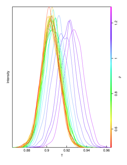
Figure 2: Distribution density of thermal fluctuations at $T=0.9$ and different densities with $N=10^{4}$ particles calculated in NVE ensemble. Density values encoded in the color key at the right side of the plot

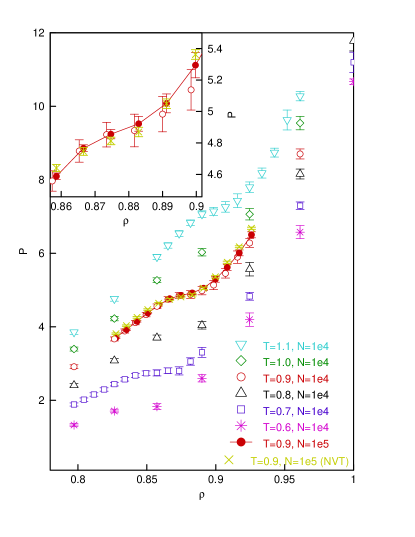
Figure 3: Equation of state at different temperatures in the vicinity of melting transition. Inset shows blow up of transition at $T=0.9$ calculated in different ensembles (implicitly assumed NVE ensemble) and various numbers of particles $N$ (see list in the main panel).

To test these assumptions we have chosen the two dimensional Lennard-Jones (2DLJ) system. Beside its archetypical character in computer simulations, its type of crystal melting attracts much attention . Original general theory of 2D crystal described in the seventieth in the works later contributed to the Berezinskii-Kosterlitz-Thouless-Halperin-Nelson-Young theory suggests that melting is infinite-order, two-stage transition between crystal and liquid (the first stage – crystal to hexatic phase transition with the loss of translational order, and the second stage – hexatic to liquid, with the loss of orientation order, see e.g. Ryzhov et al. (2023)). For simplicity we will call it continuous model. However, almost immediately this model was challenged by computer simulation study Barker et al. (1981) suggesting first order phase transition in 2DLJ system. Subsequently this system was addressed in the number of works Frenkel and McTague (1979); Toxvaerd (1981); Tobochnik and Chester (1982); Koch and Abraham (1983); Bakker et al. (1984); Udink and van der Elsken (1987); Chen et al. (1995); Somer et al. (1997, 1998) which produced controversial opinions ranging from first-order to continuous character of melting transition. Hot debates followed through 1980-1990s but did not lead to a clear conclusion. Echoes of the debates continue until recentlyWierschem and Manousakis (2010); Patashinski et al. (2010); Wierschem and Manousakis (2011); Tsiok et al. (2022). Still, it is worth mentioning that first order was predicted by the authors who used rather a small system $N<10^{4}$ particles, continuous transition was claimed by the authors who used a larger system up to $N=10^{5}$ and intermediate position was taken by authors for the system with $N=2500$ particles Patashinski et al. (2010). The most recent paper using $N=512^{2}$ particles Tsiok et al. (2022) was in favor of first-order transition. It seems that authors’ decisions are unconsciously influenced by scale of fluctuations . Most important of them are pressure fluctuations which influence the shape of equation of state (P-V) curve. Usually the presence of van-der-Waals loops on the P-V curve (or equivalently the Mayer-Wood loop on $P-\rho$ where $\rho$ is numerical density ) is considered a decisive indicator of the first order transition. Still, the depth of the loops reported in many of the works cited, is rather shallow and does not allow to make a decision in favor of first-order or continuous phase transition . The most convincing would be comparison of the effect observed with the inherent system noise due to thermal fluctuations.

We tested validity of theoretical predictions by computations with classical molecular dynamics simulations of 2DLJ system as implemented in LAMMPS software package Plimpton (1995); Plimpton et al. . Input files from Carsten Svaneborg group home page cs: were adapted to our needs. We used NVE ensemble with Langevin thermal dynamics with time step 0.01 LJ units. We used $510^{4}$ steps for thermal equilibration and next $510^{4}$ steps for estimation of thermodynamic parameters and their fluctuations . Validity of this choice will be explained later. As a rule we used $N=10^{4}$ particles. Some of the results were checked with larger system containing $N=10^{5}$ particles. Also longer simulation times and NVT ensemble were used. Initial configuration of particles was purely random. Changing the ensemble to NVT with Nose-Hoover thermostat slightly influenced the result making the system fluctuate around initially set temperature but the amplitude of fluctuations did not change. Starting configuration of particles was chosen random with ititial minimization of energy to avoid overlapping particles. The temperature varied in the range $T=0.6-1.1$ with step 0.1 and density range $\rho=0.55-1.25$. To compare our findings with previous results the temperature $T=3.0$ near the melting transition was investigated . The distribution density of thermal fluctuations was estimated by density function with default parameters as implemented in R software package R Core Team (2012).

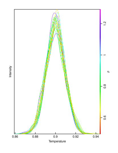
Figure 4: Distribution density of thermal fluctuations at $T=0.9$ and different densities with $N=10^{4}$ particles calculated in NVT ensemble. Density values encoded in the color key at the right side of the plot

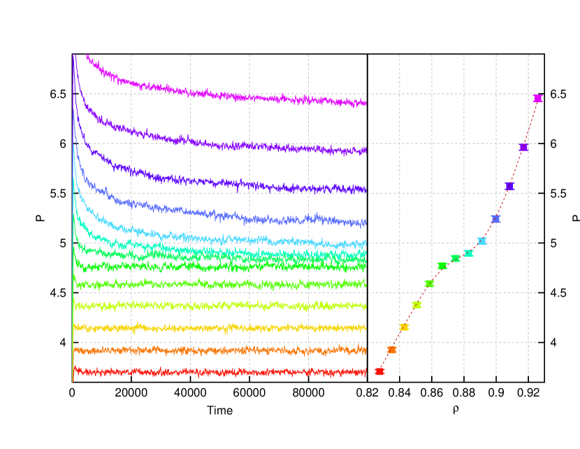
Figure 5: Fluctuations of pressure in vicinity of melting transition at $T=0.9$ (left panel) and corresponding equation of state (right panel) for larger ensemble with $N=10^{5}$ particles.

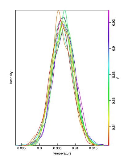
Figure 6: Distribution density of thermal fluctuations in vicinity of melting transition at $T=0.9$ and different densities for larger ensemble with $N=10^{5}$ particles. The densities values are encoded in the color key at the right side of the plot.

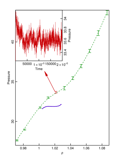
Figure 7: Equation of state in vicinity of melting temperature calculated in the current work for NVE ensemble with $N=10^{5}$ particles at $T=3.0$ (green dashed curve is guide to the eyes). Blue curve is the data for NVT ensemble for $N=256^{2}$ particles at the same temperature obtained in Ref. Tsiok et al. (2022). Inset shows fluctuations of temperature for the chosen (marked in red) point in the middle of the melting transition.

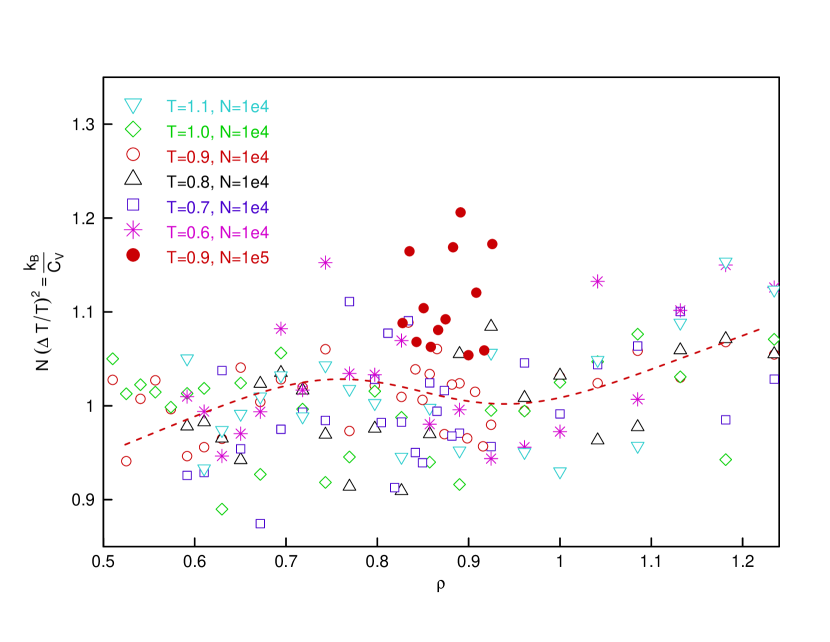
Figure 8: Heat capacity of the 2DLJ system estimated from thermal fluctuations. Dashed curve is guide to the eyes.

Fluctuations of pressure and temperature of system with $N=10^{4}$ particles at T=0.9 are shown in Fig. 1 at the same set temperature $T\approx 0.9$ and different densities ($\rho=1.23$ and $\rho=0.86$) which correspond to part of the transition deep inside the crystal phase and the liquid part just below the transition. As it was expected, fluctuations of temperature reach about 1% with almost normal distribution (see Fig. 2). The P-$\rho$ curves in vicinity of these density-temperature conditions (near the melting transition) are shown in Fig. 3. It is clear, that no van-der-Waals loops are observed in this region and with precision of pressure fluctuations might be considered as monotonous function increasing with the density rise. Still we need to inspect fluctuations of temperature to make decisive conclusions.

As it is clear from distribution functions of temperature along nominal isotherm $T=0.9$ (see Fig. 2) there is distinctive shift of temperatures to higher values of temperature than the one initially set at densities corresponding to solid state of the 2DLJ system. When approaching the melting transition this curve at $\rho\approx 1$ exhibits a clear crossover to lower temperatures and at these densities distribution curve is clearly bimodal. Presumably this is due to the ensemble (NVE) chosen by us where the energy of the system is kept constant but not the temperature, and slow pressure relaxation in the crystal phase (see Fig. 1) leads to deviation of temperature from the set value. Therefore temperature can not relax fast enough to follow temperature of the heat bath governed by Langevin dynamics. Still, we should stress that near melting transition the mean value of the temperature distribution function is constant and only slightly shifts above initially set value which is independent of density values.

For comparison we provide distributions densities obtained for the same number of particles in the same conditions but calculated in the NVT ensemble. As expected for this sort of ensemble the distribution maximum (mean value) is closer to the initially set temperature value. However, the standard deviation is almost the same as in NVE ensemble. Beside that is interesting to note that at $\rho\approx 1$ the distribution is also bimodal. This fact possibly catches an important feature in the dynamic of the system presumably arising from transition from the crystal to hexatic phase.

To demonstrate this idea we provide the results for the larger NVE ensemble with $N=10^{5}$ particles at the same temperature $T=0.9$ in the nearest vicinity of the transition (see Fig. 5). As expected, with the increase of the particles number, the values of temperature and pressure fluctuations are diminished but the slow relaxation of pressure is conserved in the crystal part of transition. However, at the upper half of time range investigated the relaxation almost reaches its equilibrium value which is demonstrated by the density distribution of temperature fluctuations in this time region (see Fig. 6). It is clear that mean temperature is only slightly above the initially set one and the drift of the mean temperature is negligible in comparison to the standard deviation of fluctuations. This means that the absence of the van-der-Waals loops on the pressure-density curve observed in Fig. 5 is not related to the drift of temperature at higher densities.

To compare our findings with previous results  Tsiok et al. (2022) we performed calculation at higher temperature T=3.0 in NVE ensemble and $N=10^{5}$ particles (see Fig. 7). In the work of Tsiok et al. Tsiok et al. (2022) calculation was done in NVT ensemble at the same temperature, but with larger particle number of $N=256^{2}$. It was stated there that the van-der-Waals loops were observed, which demonstrate first-order phase transition at least at one stage of transition (hexatic-liquid one). Still, the van-der-Waals loop observed there had rather small amplitude (in Fig. 7 it looks like a plateau), being significantly smaller than the standard deviations of pressure fluctuations calculated by us. So, there is not enough evidence of a first order of hexatic-liquid transition to overthrow existing theory of 2D melting. By the way fluctuations observed in the middle of transition, shown in the inset of Fig. 7 demonstrate convergence of pressure relaxation at longer time range ($t=210^{5}$). From this demonstration it is evident that the time range used by us (upper half of $t=10^{5}$ range) is large enough to fully converge pressure values in vicinity of the melting transition.

There is qualitative difference between the two curves in Fig. 7 – the plateau on the curve of Tsiok et al. Tsiok et al. (2022) is not only flatter than the one reported in present work, but also spans a longer range of densities $\rho$. To explain this discrepancy, we can refer to the difference between initial conditions in our work and Ref. Tsiok et al. (2022). In our setup initial atom coordinates were purely random but in Ref. Tsiok et al. (2022) they started from ideal triangular lattice. The latter case favors stability of the crystal phase, so it persists longer below melting transitions which results in van-der-Waals loops on equation of state curve. Flatness of this curve depends on the number of particles in the system so at the thermodynamic limit (the infinite number of particles) the van-der-Waals loop is believed to transform into ideal plateau with zero derivative in the middle of transition. It was demonstrated for the first time for the 2DLJ system Toxvaerd (1981) that deepness of the van-der-Waals loop in the system with “crystal” initial state is correlated to the number of particles – the larger the number the flatter curve. From this work it can be learned that the amplitude of van-der-Waals loop oscillation has the same order of magnitude as system fluctuations . In Ref. Toxvaerd (1981) for $N=256$ system both values are about 10%, which corresponds to the general rule of thumb that relative fluctuations are inversely proportional to the square root of particles number.

There is another argument in favor of first-order phase transition, namely phase coexistense observed in computer experiments between hexatic and liquid phase in the region of “van-der-Waals loop” Tsiok et al. (2022). We did not investigate this problem closely but previous report obtained by Patashinskii et al. Patashinski et al. (2010) in $N=2500$ 2DLJ system demonstrates that this separation has transient character, so the regions of hexatic phase and translational disordered liquid freely transform between each other. In our opinion (we agree with authors of Ref. Patashinski et al. (2010)) taht such a transformation is an indication of continuous transition between the two phases.

There is one more argument for continuous character of transition in 2DLJ system, that is behavior of the heat capacity at constant volume $C_{V}$ during transition. It also answers the question what we can learn from finite precision of molecular dynamics experiments. According to Eq. 1 from standard deviation of relative fluctuation of temperature we can obtain $C_{V}$. This plot with respect to density $\rho$ for temperatures in the range $T=0.6-1.1$ is depicted in Fig. 8. Overall plot is rather fuzzy but for a fixed temperature (see dashed line in Fig. 8 which is a free-hand draw for $T=0.9$) we can conclude that specific heat variation is continuous across the transition. Hence we can guess that transition is continuous too. It is also interesting to check validity of the $N^{-1/2}$ scaling law for fluctuations. We plotted the data obtained for $N=10^{5}$ ensemble on the same Fig. 8. It is clear that in comparison to $N=10^{4}$ ensemble data there is small but regular discrepancy in the range of about 15%. It can be related for other inputs into fluctuations unrelated to statistical physics, for example, induced by finite precision of computer calculations. We should also mention that almost constant $C_{V}$ value during transition was obtained in the seminal work of Frenkel and McTague Frenkel and McTague (1979) although with higher value of $C_{V}$. Similar analysis of pressure fluctuations based on Eq. 2 is also possible but for integration of $(\partial P/\partial V)_{S}$ to obtain plot of adiabatic curve it requires denser grid of temperatures than used in the present paper.

To conclude we demonstrate that the van-der-Waals loops observed on equation of state of 2DLJ system which were believed before to be an indication of first order phase transition between crystal and liquid in two dimensions are at the level of noise and can not be reliably used for determination of transition’s character. The increase of the particles number used in molecular dynamics simulation can result in attenuation of standard deviation of fluctuations, but in the same time (as it was demonstrated before Toxvaerd (1981)) it results in flattening of van-der-Waals loops on equation of state curves. However, we can demonstrate with the use of scatter of temperature fluctuations that the heat capacity during transition is continuous function which corroborates continuous character of transition. Still, with increase of the number of particles used in simulations we observe small (of order 15%) deviation from the text-book scaling formula Eq. 1 which in our opinion may be attributed to causes unrelated to statistical mechanics such as by finite digit representation of numbers in computer experiments.

References

- Hickman and Mishin (2016) J. Hickman and Y. Mishin, Phys. Rev. B 94, 184311 (2016).
- Landau et al. (1980) L. Landau, L. Pitaevskii, and E. Lifshitz, Statistical Physics, Course of theoretical physics (Pergamon Press, Oxford, 1980).
- Ryzhov et al. (2023) V. N. Ryzhov, E. A. Gaiduk, E. E. Tareeva, Y. D. Fomin, and E. N. Tsiok, Journal of Experimental and Theoretical Physics 137, 125 (2023).
- Barker et al. (1981) J. Barker, D. Henderson, and F. Abraham, Physica A: Statistical Mechanics and its Applications 106, 226 (1981).
- Frenkel and McTague (1979) D. Frenkel and J. P. McTague, Phys. Rev. Lett. 42, 1632 (1979).
- Toxvaerd (1981) S. Toxvaerd, Phys. Rev. A 24, 2735 (1981).
- Tobochnik and Chester (1982) J. Tobochnik and G. V. Chester, Phys. Rev. B 25, 6778 (1982).
- Koch and Abraham (1983) S. W. Koch and F. F. Abraham, Phys. Rev. B 27, 2964 (1983).
- Bakker et al. (1984) A. F. Bakker, C. Bruin, and H. J. Hilhorst, Phys. Rev. Lett. 52, 449 (1984).
- Udink and van der Elsken (1987) C. Udink and J. van der Elsken, Phys. Rev. B 35, 279 (1987).
- Chen et al. (1995) K. Chen, T. Kaplan, and M. Mostoller, Phys. Rev. Lett. 74, 4019 (1995).
- Somer et al. (1997) F. L. Somer, G. S. Canright, T. Kaplan, K. Chen, and M. Mostoller, Phys. Rev. Lett. 79, 3431 (1997).
- Somer et al. (1998) F. L. Somer, G. S. Canright, and T. Kaplan, Phys. Rev. E 58, 5748 (1998).
- Wierschem and Manousakis (2010) K. Wierschem and E. Manousakis, Physics Procedia 3, 1515 (2010), proceedings of the 22th Workshop on Computer Simulation Studies in Condensed Matter Physics (CSP 2009).
- Patashinski et al. (2010) A. Z. Patashinski, R. Orlik, A. C. Mitus, B. A. Grzybowski, and M. A. Ratner, The Journal of Physical Chemistry C 114, 20749 (2010).
- Wierschem and Manousakis (2011) K. Wierschem and E. Manousakis, Phys. Rev. B 83, 214108 (2011).
- Tsiok et al. (2022) E. N. Tsiok, Y. D. Fomin, E. A. Gaiduk, E. E. Tareyeva, V. N. Ryzhov, P. A. Libet, N. A. Dmitryuk, N. P. Kryuchkov, and S. O. Yurchenko, The Journal of Chemical Physics 156, 114703 (2022).
- Plimpton (1995) S. Plimpton, Journal of Computational Physics 117, 1 (1995).
- (19) S. Plimpton, A. Kohlmeyer, A. Thompson, S. Moore, and R. Berger, “LAMMPS Stable release 29 September 2021,” .
- (20) “Svaneborg lab computational soft-matter group: Lammps demos,” .
- R Core Team (2012) R Core Team, “R: A language and environment for statistical computing,” (2012), ISBN 3-900051-07-0.