Counting problems in trees, with applications to fixed points of cellular automata

Abstract

Cellular automata are synchronous discrete dynamical systems used to describe complex dynamic behaviors. The dynamic is based on local interactions between the components, these are defined by a finite graph with an initial node coloring with two colors. In each step, all nodes change their current color synchronously to the least/most frequent color in their neighborhood and in case of a tie, keep their current color. After a finite number of rounds these systems either reach a fixed point or enter a 2-cycle. The problem of counting the number of fixed points for cellular automata is #P-complete. In this paper we consider cellular automata defined by a tree. We propose an algorithm with run-time $O(n\Delta)$ to count the number of fixed points, here $\Delta$ is the maximal degree of the tree. We also prove upper and lower bounds for the number of fixed points. Furthermore, we obtain corresponding results for pure cycles, i.e., instances where each node changes its color in every round. We provide examples demonstrating that the bounds are sharp. The results are proved for the minority and the majority model.

Keywords Tree cellular automata $\cdot$ Fixed points  $\cdot$ Counting problems.

1 Introduction

A widely used abstraction of classical distributed systems such as multi-agent systems are graph automata. They evolve over time according to some simple local behaviors of its components. They belong to the class of synchronous discrete-time dynamical systems. A common model is as follows: Let $G$ be a graph, where each node is initially either black or white. In discrete-time rounds, all nodes simultaneously update their color based on a predefined local rule. Locality means that the color associated with a node in round $t$ is determined by the colors of the neighboring nodes in round $t-1$. As a local rule we consider the minority and the majority rule that arises in various applications and as such have received wide attention in recent years, in particular within the context of information spreading. Such systems are also known as graph cellular automata. It is well-known [10, 20] that they always converge to configurations that correspond to cycles either of length 1 – a.k.a. fixed points – or of length 2, i.e., such systems eventually reach a stable configuration or toggle between two configurations.

One branch of research so far uses the assumption that the initial configuration is random. Questions of interest are on the expected stabilization time of this process [25] and the dominance problem [19]. Fogelman et al. proved that the stabilization time is $O(n^{2})$ [9].

In this paper we focus on counting problems related to cellular automata, in particular counting the number of fixed points and pure 2-cycles, i.e., instances where each node changes its color in every round. This research is motivated by applications of so-called Boolean networks (BN) [12], i.e., discrete-time dynamical systems, where each node (e.g., gene) takes either 0 (passive) or 1 (active) and the states of nodes change synchronously according to regulation rules given as Boolean functions. Since the problem of counting the fixed points of a BN is in general #P-complete [3, 22, 8], it is interesting to find graph classes, for which the number of fixed points can be efficiently determined. These counting problems have attracted a lot of research in recent years [6, 4, 14].

We consider tree cellular automata, i.e., the defining graphs are finite trees. The results are based on a characterization of fixed points and pure 2-cycles for tree cellular automata [23]. The authors of [23] describe algorithms to enumerate all fixed points and all pure cycles. Since the number of fixed points and pure 2-cycles can grow exponentially with the tree size, these algorithms are unsuitable to efficiently compute these numbers. We prove the following theorem.

Theorem 1.

The number of fixed points and the number of pure 2-cycles of a tree with $n$ nodes and maximal node degree $\Delta$ can be computed in time $O(n\Delta)$.

We also prove the following theorem with upper and lower bounds for the number of fixed points of a tree improving results of [23] (parameter $r$ is explained in Sec. 4.3). In the following, the $i^{th}$ Fibonacci number is denoted by $\mathbb{F}_{i}$.

Theorem 2.

A tree with $n$ nodes, diameter $D$ and maximal node degree $\Delta$ has at least $\max\left(2^{r/2+1},2\mathbb{F}_{D}\right)$ and at most $\min\left(2^{n-\Delta},2\mathbb{F}_{n-\lceil\Delta/2\rceil}\right)$ fixed points.

For the number of pure cycles we prove the following result, which considerably improves the bound of [23].

Theorem 3.

A tree with maximal degree $\Delta$ has at most $\min\left(2^{n-\Delta},2\mathbb{F}_{\lfloor n/2\rfloor}\right)$ pure 2-cycles.

We provide examples demonstrating ranges where these bounds are sharp. All results hold for the minority and the majority rule. We also formulate several conjectures about counting problems and propose future research directions.

2 State of the Art

The analysis of fixed points of minority/majority rule cellular automata received limited attention so far. Královič determined the number of fixed points of a complete binary tree for the majority process [13]. For the majority rule he showed that this number asymptotically tends to $4n(2\alpha)^{n}$, where $n$ is the number of nodes and $\alpha\approx 0.7685$. Agur et al. did the same for ring topologies [2], the number of fixed point is in the order of $\Phi^{n}$, where $\Phi=(1+\sqrt{5})/2$. In both cases the number of fixed points is an exponentially small fraction of all configurations.

A related concept are Boolean networks (BN). They have been extensively used as mathematical models of genetic regulatory networks. The number of fixed points of a BN is a key feature of its dynamical behavior. A gene is modeled by binary values, indicating two transcriptional states, active or inactive. Each network node operates by the same nonlinear majority rule, i.e., majority processes are a particular type of BN [24]. The number of fixed points is an important feature of the dynamical behavior of a BN [5]. It is a measure for the general memory storage capacity. A high number implies that a system can store a large amount of information, or, in biological terms, has a large phenotypic repertoire [1]. However, the problem of counting the fixed points of a BN is in general #P-complete [3]. There are only a few theoretical results to efficiently determine this set [11]. Aracena determined the maximum number of fixed points regulatory Boolean networks, a particular class of BN [5].

Recently, Nakar and Ron studied the dynamics of a class of synchronous one-dimensional cellular automata for the majority rule [17]. They proved that fixed points and 2-cycles have a particular spatially periodic structure and give a characterization of this structure. Concepts related to fixed points of the minority/majority process have been analyzed. A partition $(S,\bar{S})$ of the nodes of a graph is called a global defensive $0$-alliance or a monopoly if $\lvert\mskip 0.90001muN_{S}(v)\mskip 0.90001mu\rvert\geq\lvert\mskip 0.90001muN_{\bar{S}}(v)\mskip 0.90001mu\rvert$ for each node $v$ [15]. Thus, a fixed point of the minority/majority process induces a $0$-alliance (but not conversely).

Most research on discrete-time dynamical systems on graphs is focused on bounding the stabilization time. Good overviews for the majority (resp. minority) process can be found in [25] (resp. [18]). Rouquier et al. studied the minority process in the asynchronous model, i.e., not all nodes update their color concurrently [21]. They showed that the stabilization time strongly depends on the topology and observe that the case of trees is non-trivial.

2.1 Notation

Let $T=(V,E)$ be a finite, undirected tree with $n=\lvert\mskip 0.90001muV\mskip 0.90001mu\rvert$. The maximum degree of $T$ is denoted by $\Delta(T)$, the diameter by $D(T)$. The parameter $T$ is omitted in case no ambiguity arises. A star graph is a tree with $n-1$ leaves. A $l$-generalized star graph is obtained from a star graph by inserting $l-1$ nodes into each edge, i.e., $n=l\Delta+1$. For $F\subseteq E$ and $v\in V$ denote by $deg_{F}(v)$ the number of edges in $F$ incident to $v$. Note that $deg_{F}(v)\leq deg(v)$. For $i\geq 2$ denote by $E^{i}(T)$ the set of edges of $T$, where each end node has degree at least $i$. For $v\in V$ denote the set of $v$’s neighbors by $N(v)$. For $e=(v_{1},v_{2})\in E^{2}(T)$ let $T_{i}$ be the subtree of $T$ consisting of $e$ and the connected component of $T\setminus e$ that contains $v_{i}$. We call $T_{i}$ the constituents of $T$ for $e$. $T_{1}$ and $T_{2}$ together have $n+2$ nodes. We denote the $i^{th}$ Fibonacci number by $\mathbb{F}_{i}$, i.e., $\mathbb{F}_{0}=0,\mathbb{F}_{1}=1$, and $\mathbb{F}_{i}=\mathbb{F}_{i-1}+\mathbb{F}_{i-2}$.

3 Synchronous Discrete-Time Dynamical Systems

Let $G=(V,E)$ be a finite, undirected graph. A coloring $c$ assigns to each node of $G$ a value in $\{0,1\}$ with no further constraints on $c$. Denote by $\mathcal{C}(G)$ the set of all colorings of $G$, i.e., $\lvert\mskip 0.90001mu\mathcal{C}(G)\mskip 0.90001mu\rvert=2^{\lvert\mskip 0.90001muV\mskip 0.90001mu\rvert}$. A transition process $\mathcal{M}$ is a mapping $\mathcal{M}:\mathcal{C}(G)\longrightarrow\mathcal{C}(G)$. Given an initial coloring $c$, a transition process produces a sequence of colorings $c,\mathcal{M}(c),\mathcal{M}(\mathcal{M}(c)),\ldots$. We consider two transition processes: Minority and Majority and denote the corresponding mappings by $\mathcal{MIN}$ and $\mathcal{MAJ}$. They are local mappings in the sense that the new color of a node is based on the current colors of its neighbors. To determine $\mathcal{M}(c)$ the local mapping is executed in every round concurrently by all nodes. In the minority (resp. majority) process each node adopts the minority (resp. majority) color among all neighbors. In case of a tie the color remains unchanged (see Fig. 1). Formally, the minority process is defined for a node $v$ as follows:

$$\mathcal{MIN}(c)(v)=\begin{cases}c(v)&\text{if }\lvert\mskip 0.90001muN^{c(v)}(v)\mskip 0.90001mu\rvert\leq\lvert\mskip 0.90001muN^{1-c(v)}(v)\mskip 0.90001mu\rvert\\ 1-c(v)&\text{if }\lvert\mskip 0.90001muN^{c(v)}(v)\mskip 0.90001mu\rvert>\lvert\mskip 0.90001muN^{1-c(v)}(v)\mskip 0.90001mu\rvert\end{cases}$$

$N^{i}(v)$ denotes the set of $v$’s neighbors with color $i$ ($i=0,1$). The definition of $\mathcal{MAJ}$ is similar, only the binary operators $\leq$ and $>$ are reversed. Some results hold for both the minority and the majority process. To simplify notation we use the symbol $\mathcal{{M}}$ as a placeholder for $\mathcal{{MIN}}$ and $\mathcal{{MAJ}}$.

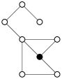
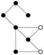
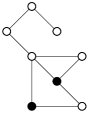
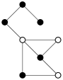
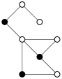
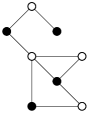
Figure 1: For the coloring on the left $\mathcal{{MIN}}$ reaches after 5 rounds a fixed point. $\mathcal{{MAJ}}$ reaches for the same initial coloring after one round a monochromatic coloring.

Let $c\in\mathcal{C}(G)$. If $\mathcal{M}(c)=c$ then $c$ is called a fixed point. It is called a 2-cycle if $\mathcal{M}(c)\not=c$ and $\mathcal{M}(\mathcal{M}(c))=c$. A 2-cycle is called pure if $\mathcal{M}(c)(v)\not=c(v)$ for each node $v$ of $G$, see Fig. 2. Denote by $\mathcal{F}_{\mathcal{M}}(G)$ (resp. $\mathcal{P}_{\mathcal{M}}(G)$) the set of all $c\in\mathcal{C}(G)$ that constitute a fixed point (resp. a pure 2-cycle) for $\mathcal{M}$.

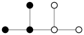
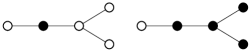
Figure 2: Examples for the $\mathcal{MIN}$ rule. The coloring of the first (resp. second) tree is a fixed point (resp. a pure 2-cycle). The right two colorings are a non-pure 2-cycle.

Let $T$ be a tree. The following results are based on a characterization of $\mathcal{F}_{\mathcal{M}}(T)$ and $\mathcal{P}_{\mathcal{M}}(T)$ by means of subsets of $E(T)$ [23]. Let $E_{fix}(T)$ be the set of all $\mathcal{F}$-legal subsets of $E(T)$, where $F\subseteq E(T)$ is $\mathcal{F}$-legal if $2deg_{F}(v)\leq deg(v)$ for each $v\in V$. Each $\mathcal{F}$-legal set is contained in $E^{2}(T)$, hence $\lvert\mskip 0.90001muE_{fix}(T)\mskip 0.90001mu\rvert\leq 2^{\lvert\mskip 0.90001muE^{2}(T)\mskip 0.90001mu\rvert}$. Theorem 1 of [23] proves that $\lvert\mskip 0.90001mu\mathcal{F}_{\mathcal{M}}(T)\mskip 0.90001mu\rvert=2\lvert\mskip 0.90001muE_{fix}(T)\mskip 0.90001mu\rvert$, see Fig. 3. Let $E_{pure}(T)$ be the set of all $\mathcal{P}$-legal subsets of $E(T)$, where $F\subseteq E(T)$ is $\mathcal{P}$-legal if $2deg_{F}(v)<deg(v)$ for each $v\in V$. Thus, $\mathcal{P}$-legal subsets are contained in $E^{3}(T)$ and therefore $\lvert\mskip 0.90001muE_{pure}(T)\mskip 0.90001mu\rvert\leq 2^{\lvert\mskip 0.90001muE^{3}(T)\mskip 0.90001mu\rvert}$. Theorem 4 of [23] proves that $\lvert\mskip 0.90001mu\mathcal{P}_{\mathcal{M}}(T)\mskip 0.90001mu\rvert=2\lvert\mskip 0.90001muE_{pure}(T)\mskip 0.90001mu\rvert$. For the tree in Fig. 3 we have $E_{pure}(T)=\{\emptyset\}$, thus $\lvert\mskip 0.90001mu\mathcal{P}_{\mathcal{M}}(T)\mskip 0.90001mu\rvert=2$. The pure colorings are the two monochromatic colorings. Given these results it is unnecessary to treat $\mathcal{{MIN}}$ and $\mathcal{{MAJ}}$ separately. To determine the number of fixed points (resp. pure 2-cycles) it suffices to compute $\lvert\mskip 0.90001muE_{fix}(T)\mskip 0.90001mu\rvert$ (resp. $\lvert\mskip 0.90001muE_{pure}(T)\mskip 0.90001mu\rvert$).

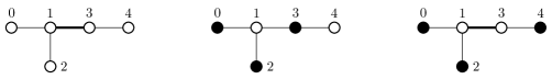
Figure 3: A tree $T$ with $E_{fix}(T)=\{\emptyset,\{(1,3)\}\}$ and the corresponding fixed points for $\mathcal{MIN}$, the other two can be obtained by inverting colors.

4 Fixed Points

In this section we propose an efficient algorithm to determine $\lvert\mskip 0.90001mu\mathcal{F}_{\mathcal{M}}(T)\mskip 0.90001mu\rvert$, we provide upper and lower bounds for $\lvert\mskip 0.90001mu\mathcal{F}_{\mathcal{M}}(T)\mskip 0.90001mu\rvert$ in terms of $n$, $\Delta$, and $D$, and discuss the quality of these bounds. As stated above, it suffices to consider $E_{fix}(T)$ and there is no need to distinguish the minority and the majority model. The following lemma is crucial for our results. It allows to recursively compute $\lvert\mskip 0.90001muE_{fix}(T)\mskip 0.90001mu\rvert$. For a node $v$ define

$$E_{fix}(T,v)=\{F\in E_{fix}(T)\;|\;2(deg_{F}(v)+1)\leq deg(v)\}.$$

Lemma 4.

Let $T$ be a tree, $e=(v_{1},v_{2})\in E^{2}(T)$, and $T_{i}$ the constituents of $T$ for $e$. Then $\lvert\mskip 0.90001muE_{fix}(T)\mskip 0.90001mu\rvert=\lvert\mskip 0.90001muE_{fix}(T_{1},v_{1})\mskip 0.90001mu\rvert\lvert\mskip 0.90001muE_{fix}(T_{2},v_{2})\mskip 0.90001mu\rvert+\lvert\mskip 0.90001muE_{fix}(T_{1})\mskip 0.90001mu\rvert\lvert\mskip 0.90001muE_{fix}(T_{2})\mskip 0.90001mu\rvert$.

Proof.

Let $A=\{F\in E_{fix}(T)\;|\;e\in F\}$ and $B=\{F\in E_{fix}(T)\;|\;e\not\in F\}$. Then

$$A\cap B=\emptyset\text{ and }A\cup B=E_{fix}(T),$$

i.e., $\lvert\mskip 0.90001muE_{fix}(T)\mskip 0.90001mu\rvert=\lvert\mskip 0.90001muA\mskip 0.90001mu\rvert+\lvert\mskip 0.90001muB\mskip 0.90001mu\rvert$. If $F\in A$ then $F\setminus e\cap T_{i}\in E_{fix}(T_{i},v_{i})$ since $T_{1}\cap T_{2}=\{e\}$. Hence, $\lvert\mskip 0.90001muA\mskip 0.90001mu\rvert\leq\lvert\mskip 0.90001muE_{fix}(T_{1},v_{1})\mskip 0.90001mu\rvert\lvert\mskip 0.90001muE_{fix}(T_{2},v_{2})\mskip 0.90001mu\rvert$. If $F\in B$ then $F\cap T_{i}\in E_{fix}(T_{i})$, i.e., $\lvert\mskip 0.90001muB\mskip 0.90001mu\rvert\leq\lvert\mskip 0.90001muE_{fix}(T_{1})\mskip 0.90001mu\rvert\lvert\mskip 0.90001muE_{fix}(T_{2})\mskip 0.90001mu\rvert$. This yields,

$$\lvert\mskip 0.90001muE_{fix}(T)\mskip 0.90001mu\rvert\leq\lvert\mskip 0.90001muE_{fix}(T_{1},v_{1})\mskip 0.90001mu\rvert\lvert\mskip 0.90001muE_{fix}(T_{2},v_{2})\mskip 0.90001mu\rvert+\lvert\mskip 0.90001muE_{fix}(T_{1})\mskip 0.90001mu\rvert\lvert\mskip 0.90001muE_{fix}(T_{2})\mskip 0.90001mu\rvert.$$

If $F_{i}\in E_{fix}(T_{i},v_{i})$, then $F_{1}\cup F_{2}\cup\{e\}\in A$. If $F_{i}\in E_{fix}(T_{i})$, then $F_{1}\cup F_{2}\in B$. Hence,

$$\lvert\mskip 0.90001muE_{fix}(T_{1},v_{1})\mskip 0.90001mu\rvert\lvert\mskip 0.90001muE_{fix}(T_{2},v_{2})\mskip 0.90001mu\rvert+\lvert\mskip 0.90001muE_{fix}(T_{1})\mskip 0.90001mu\rvert\lvert\mskip 0.90001muE_{fix}(T_{2})\mskip 0.90001mu\rvert\leq\lvert\mskip 0.90001muE_{fix}(T)\mskip 0.90001mu\rvert.$$

∎

If $deg_{T}(v_{i})\equiv 0(2)$, then $E_{fix}(T_{i},v_{i})=E_{fix}(T_{i}\!\setminus\!\{v_{i}\})$. This yields a corollary.

Corollary 5.

Let $P_{n}$ be a path with $n$ nodes, then $\lvert\mskip 0.90001muE_{fix}(P_{n})\mskip 0.90001mu\rvert=F_{n-1}$.

4.1 Computing $\lvert\mskip 0.90001mu\mathcal{F}_{\mathcal{M}}(T)\mskip 0.90001mu\rvert$

Algorithm 1 of [23] enumerates all elements of $E_{fix}(T)$ for a tree $T$. Since $\lvert\mskip 0.90001muE_{fix}(T)\mskip 0.90001mu\rvert$ can grow exponentially with the size of $T$, it is unsuitable to efficiently determine $\lvert\mskip 0.90001muE_{fix}(T)\mskip 0.90001mu\rvert$. In this section we propose an efficient novel algorithm to compute $\lvert\mskip 0.90001muE_{fix}(T)\mskip 0.90001mu\rvert$ in time $O(n\Delta)$ based on Lemma 4. The algorithm operates in several steps. Let us define the input for the algorithm. First, each node $v_{i}$ is annotated with $b_{i}=\lfloor deg(v_{i})/2\rfloor$. Let $T_{R}$ be the tree obtained form $T$ by removing all leaves of $T$; denote by $t$ the number of nodes of $T_{R}$. Select a node of $T_{R}$ as a root and assign numbers $1,\ldots,t$ to nodes in $T_{R}$ using a postorder depth-first search. Direct all edges towards higher numbers, i.e., the numbers of all predecessors of a node $i$ are smaller than $i$, see Fig. 4 for an example. The annotated rooted tree $T_{R}$ is the input to Algorithm 1.

Figure 4: From left to right: Tree $T$, annotation of $T$, $T_{R}$, a postorder numbering of $T_{R}$.

Algorithm 1 recursively operates on two types of subtrees of $T_{R}$ which are defined next. For $k=1,\ldots,t-1$ denote by $T_{k}$ the subtree of $T_{R}$ consisting of $k$’s parent together with all nodes connected to $k$’s parent by paths using only nodes with numbers at most $k$ (see Fig. 5). Note that $T_{R}=T_{t-1}$. For $k=1,\ldots,t$ denote by $S_{k}$ the subtree of $T_{R}$ consisting of all nodes from which node $k$ can be reached. In particular $S_{t}=T_{R}$, and if $k$ is a leaf then $S_{k}$ consist of node $k$ only.

Figure 5: The subtrees $T_{1},\ldots T_{7}$ of the tree from Fig. 4. Note that $S_{4}=T_{3}$ and $S_{3}$ consists of node $3$ only.

For a subtree $S$ of $T_{R}$ with largest node $s$ and $b\geq 0$ denote by $w(S,b)$ the number of subsets $F$ of $E(S)$ with $deg_{F}(i)\leq b_{i}$ for all nodes $i$ of $S$ (recall that $b_{i}$ is defined above) and $deg_{F}(s)\leq b$. Let $w(S,-1)=0$. Clearly if $b\geq b_{s}$ then $w(S,b)=w(S,b_{s})$. If $S$ consists of a single node $s$ then $s$ is a leaf and $E(S)=\emptyset$; therefore $w(S,b)=1$ for all $b\geq 0$. Note that $w(S,b_{s}-1)=\lvert\mskip 0.90001muE_{fix}(S,s)\mskip 0.90001mu\rvert$. The following observation shows the relation between $\lvert\mskip 0.90001muE_{fix}(T)\mskip 0.90001mu\rvert$ and $w(T_{k},b)$.

Lemma 6.

$\lvert\mskip 0.90001muE_{fix}(T)\mskip 0.90001mu\rvert=w(T_{t-1},b_{t})$ for any tree $T$.

The next lemma shows how to recursively compute $w(T_{k},b)$ using Lemma 4.

Lemma 7.

Let $i$ be an inner node of $T_{R}$, $k$ a child of $i$, and $b\geq 0$. Let $\delta_{b,0}=0$ if $b=0$ and $1$ otherwise. If $k$ is the smallest child of $i$, then

$$w(T_{k},b)=w(S_{k},b_{k})+w(S_{k},b_{k}-1)\delta_{b,0}.$$

Otherwise let $j\not=k$ be the largest child of $i$ such that $j<k$. Then

$$w(T_{k},b)=w(T_{j},b)w(S_{k},b_{k})+w(T_{j},b-1)w(S_{k},b_{k}-1).$$

Proof.

The proof for both cases is by induction on $k$. Consider the first case. If $k$ is a leaf then $w(S_{k},b)=1$ for all $b\geq 0$ and $w(S_{k},-1)=0$. This is the base case. Assume $k$ is not a leaf. $T_{k}$ consists of node $i$, $S_{k}$ and the edge $e=(i,k)$. If $b=0$ then $\delta_{b,0}=0$ and $w(T_{k},0)=w(S_{k},b_{k})$ by definition. Let $b>0$, i.e., $\delta_{b,0}=1$. Let $f_{i}$ (resp. $f_{o}$) be the number of $F\subseteq E(T_{k})$ with $deg_{F}(l)\leq b_{l}$ for all nodes $l$ of $T_{k}$, $deg_{F}(i)\leq b$ and $e\in F$ (resp. $e\not\in F$). Let $F\subseteq E(T_{k})$. If $e\in F$ let $\hat{F}=F\setminus e$. Then $\hat{F}\in E(S_{k})$, $deg_{\hat{F}}(l)\leq b_{l}$ for all nodes $l\not=k$ in $S_{k}$ and $deg_{\hat{F}}(k)\leq b_{k}-1$, hence $f_{i}\leq w(S_{k},b_{k}-1)$. If $e\not\in F$ then $F\in E(S_{k})$ and $deg_{F}(l)\leq b_{l}$ for all nodes $l$ in $S_{k}$, hence $f_{o}\leq w(S_{k},b_{k})$. Thus,

$$w(T_{k},b)\leq w(S_{k},b_{k})+w(S_{k},b_{k}-1).$$

On the other hand, let $F\in E(S_{k})$ such that $deg_{F}(l)\leq b_{l}$ for all nodes $l\not=k$ in $S_{k}$. If $deg_{F}(k)\leq b_{k}-1$ then $F\cup\{e\}$ contributes to $w(T_{k},b)$ and if $deg_{F}(k)\leq b_{k}$ then $F$ contributes to $w(T_{k},b)$. Thus

$$w(T_{k},b)\geq w(S_{k},b_{k})+w(S_{k},b_{k}-1).$$

Consider the second statement. The case that $k$ is a leaf follows immediately from Lemma 4. Assume that $k$ is not a leaf. We apply Lemma 4 to $T_{k}$ and edge $(i,k)$. Then $T_{j}\cup(i,k)$ and $S_{k}\cup(i,k)$ are the constituents of $T_{k}$. Note that $E_{fix}(S_{k}\cup(i,k),i)=w(S_{k},b_{k}-1)$ and $E_{fix}(T_{j}\cup(i,k),k)=w(T_{j},b-1)$.∎

for $b=0,\dots,B$ do

       $W(0,b)=1$

      

for $k=1,\dots,t-1$ do

       if $k$ is the smallest child of its parent in $T_{R}$ then

             $W(k,0):=W(l(k),b_{k})$

             for $b=1,\dots,B$ do

                   $W(k,b):=W(l(k),b_{k})+W(l(k),b_{k}-1)$

                  

            

       else

             let $j$ be the largest sibling of $k$ with $j<k$ in $T_{R}$

             $W(k,0):=W(j,0)W(l(k),b_{k})$

             for $b=1,\dots,B$ do

                   $W(k,b):=W(j,b)W(l(k),b_{k})+W(j,b-1)W(l(k),b_{k}-1)$

                  

            

      

Algorithm 1 Computation of $W(k,b)$ for all $k$ and $b$ using $T_{R}$.

Algorithm 1 makes use of Lemma 6 and 7 to determine $w(T_{t-1},b_{t})$, which is equal to $\lvert\mskip 0.90001muE_{fix}(T)\mskip 0.90001mu\rvert$. Let $B=\max\{b_{i}\;|\;i=1,\ldots,t\}$, clearly $B\leq\Delta/2$. Algorithm 1 uses an array $W$ of size $[0,t-1]\times[0,B]$ to store the values of $w(\cdot,\cdot)$. The first index is used to identify the tree $T_{k}$. To simplify notation this index can also have the value $0$. To store the values of $w(S_{k},b)$ in the same array we define for each inner node $k$ an index $l(k)$ as follows $l(k)=k-1$ if $k$ is not a leaf and $l(k)=0$ otherwise. Then clearly $S_{k}=T_{l(k)}$ if $k$ is not a leaf. More importantly, the value of $w(S_{k},b)$ is stored in $W({l(k)},b)$ for all $k$ and $b$.

The algorithm computes the values of $W$ for increasing values of $k<t$ beginning with $k=0$. If $W(j,b)$ is known for all $j<k$ and all $b\in[0,B]$ we can simply compute $W(k,b)$ for all values of $b$ in $[0,B]$ using the equations of Lemma 7. Finally we have $w(t-1,b_{t})$ which is equal to $\lvert\mskip 0.90001muE_{fix}(T)\mskip 0.90001mu\rvert$. See Appendix A for an execution of Algorithm 1. Theorem 1 follows from Lemma 6 and 7.

4.2 Upper Bounds for $\lvert\mskip 0.90001mu\mathcal{F}_{\mathcal{M}}(T)\mskip 0.90001mu\rvert$

The definition of $E_{fix}(T)$ immediately leads to a first upper bound for $\lvert\mskip 0.90001mu\mathcal{F}_{\mathcal{M}}(T)\mskip 0.90001mu\rvert$.

Lemma 8.

$\lvert\mskip 0.90001muE_{fix}(T)\mskip 0.90001mu\rvert\leq 2^{n-\Delta-1}$.

Proof.

Theorem 1 of [23] implies $\lvert\mskip 0.90001muE_{fix}(T)\mskip 0.90001mu\rvert\leq 2^{\lvert\mskip 0.90001muE^{2}(T)\mskip 0.90001mu\rvert}$. Note that $\lvert\mskip 0.90001muE^{2}(T)\mskip 0.90001mu\rvert=n-1-l$, where $l$ is the number of leaves of $T$. It is well known that $l=2+\sum_{j=3}^{\Delta}(j-2)D_{j}$, where $D_{j}$ denotes the number of nodes with degree $j$. Thus,

$$\hskip 19.91692pt\lvert\mskip 0.90001muE^{2}(T)\mskip 0.90001mu\rvert=n-3-\sum_{j=3}^{\Delta}(j-2)D_{j}\leq n-3-(\Delta-2)=n-\Delta-1.\hskip 42.67912pt$$

∎

For $\Delta<n-\lceil n/3\rceil$ the bound of Lemma 8 is not attained. Consider the case $n=8,\Delta=4$. The tree from Fig. 6 with $x=1$ has $14$ fixed points, this is the maximal attainable value.

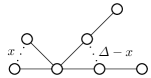
Figure 6: If $x\geq\Delta/2$ then $\lvert\mskip 0.90001mu\mathcal{F}_{\mathcal{M}}(T)\mskip 0.90001mu\rvert=2^{n-\Delta}$.

For $\Delta<n/2$ we will prove a much better bound than that of Lemma 8. For this we need the following technical result.

Lemma 9.

Let $T=(V,E)$ be a tree with a single node $v$ that has degree larger than $2$. Let ${\cal D}=[dist(w,v)\;|\;w\in V,w\not=v]$ be the multi-set with the distances of all nodes to $v$. Then

$$\lvert\mskip 0.90001muE_{fix}(T)\mskip 0.90001mu\rvert=\sum_{S\subset{\cal D},\lvert\mskip 0.90001muS\mskip 0.90001mu\rvert\leq\Delta/2}\leavevmode\nobreak\ \prod_{s\in S}\mathbb{F}_{s-1}\prod_{s\in{\cal D}\setminus S}\mathbb{F}_{s}.$$

Proof.

Let ${\cal P}$ be the set of all $\Delta$ paths from $v$ to a leaf of $T$. Let $F\in E_{fix}(T)$ and

$${\cal P}_{F}=\{P\in{\cal P}\;|\;F\cap P\not\in E_{fix}(P)\}.$$

Let $P\in{\cal P}_{F}$ and $v_{P}$ the node of $P$ adjacent to $v$. Then $(v,v_{P})\in F$. This yields $\lvert\mskip 0.90001mu{\cal P}_{F}\mskip 0.90001mu\rvert\leq\Delta/2$. For $P\in{\cal P}$ let $\hat{P}$ be an extension of $P$ by an edge $(v,x)$ with a new node $x$. Then $F\cap P\in E_{fix}(\hat{P})$ for each $P\in{\cal P}_{F}$. By Cor. 5 there are $\mathbb{F}_{\lvert\mskip 0.90001muP\mskip 0.90001mu\rvert-2}$ possibilities for $F\cap P$. Let $\bar{{\cal P}}_{F}={\cal P}\setminus{\cal P}_{F}$. For $P\in\bar{{\cal P}}_{F}$ we have $(v,v_{P})\not\in F$. Hence, $F\cap P\in E_{fix}(P)$. By Cor. 5 there are $\mathbb{F}_{\lvert\mskip 0.90001muP\mskip 0.90001mu\rvert-1}$ possibilities for $F\cap P$. Also $\lvert\mskip 0.90001mu\bar{{\cal P}}_{F}\mskip 0.90001mu\rvert=\Delta-\lvert\mskip 0.90001mu{\cal P}_{F}\mskip 0.90001mu\rvert$.

Let ${\cal P}_{1}\subset{\cal P}$ with $\lvert\mskip 0.90001mu{\cal P}_{1}\mskip 0.90001mu\rvert\leq\Delta/2$ and $\hat{F}_{P}\in E_{fix}(\hat{P})$ for all $P\in{\cal P}_{1}$ and $F_{P}\in E_{fix}(P)$ for all $P\in{\cal P}\setminus{\cal P}_{1}$. Then the union of all $\hat{F}_{P}$ and all $F_{P}$ is a member of $E_{fix}(T)$. This yields the result. ∎

Corollary 10.

Let $T$ be a $l$-generalized star graph. Then

$$\lvert\mskip 0.90001muE_{fix}(T)\mskip 0.90001mu\rvert=\sum_{i=0}^{\lfloor\Delta/2\rfloor}\binom{\Delta}{i}\mathbb{F}_{l-1}^{i}\mathbb{F}_{l}^{\Delta-i}.$$

The corollary yields that a star graph (i.e. $l=1$) has two fixed points. For $l=2$ we have the following result.

Lemma 11.

Let $T$ be a $2$-generalized star graph. Then $\lvert\mskip 0.90001muE_{fix}(T)\mskip 0.90001mu\rvert\leq\mathbb{F}_{n-\lceil\Delta/2\rceil}$.

Proof.

We use Corollary 10. If $\Delta\equiv 0(2)$ then

$$\lvert\mskip 0.90001muE_{fix}(T)\mskip 0.90001mu\rvert=\sum_{i=0}^{\lfloor\Delta/2\rfloor}\binom{\Delta}{i}=\frac{1}{2}\left(2^{\Delta}+\binom{\Delta}{\Delta/2}\right)\leq\mathbb{F}_{3\Delta/2+1}=\mathbb{F}_{n-\Delta/2},$$

otherwise $\lvert\mskip 0.90001muE_{fix}(T)\mskip 0.90001mu\rvert=2^{\Delta-1}\leq\mathbb{F}_{n-\lceil\Delta/2\rceil}$. ∎

In Theorem 2 we prove that the upper bound of Lemma 11 holds for all trees. First, we prove two technical results.

Lemma 12.

Let $T$ be a tree and $v$ a leaf of $T$ with neighbor $w$. Let $n_{l}$ (resp. $n_{i}$) be the number of neighbors of $w$ that are leaves (resp. inner nodes). If $n_{l}>n_{i}$ then $E_{fix}(T)=E_{fix}(T\setminus v)$.

Proof.

Clearly, $E_{fix}(T\setminus v)\subseteq E_{fix}(T)$. Let $F\in E_{fix}(T)$. Then $deg_{F}(w)\leq n_{i}$. Thus, $2deg_{F}(w)\leq 2n_{i}\leq n_{l}-1+n_{i}=deg_{T}(w)-1$. Hence, $F\in E_{fix}(T\setminus v)$, i.e., $E_{fix}(T)\subseteq E_{fix}(T\setminus v)$. ∎

Lemma 13.

Let $T$ be a tree and $v,w,u$ a path with $deg(v)=1$ and $deg(w)=2$. Then $\lvert\mskip 0.90001muE_{fix}(T)\mskip 0.90001mu\rvert\leq\lvert\mskip 0.90001muE_{fix}(T_{v})\mskip 0.90001mu\rvert+\lvert\mskip 0.90001muE_{fix}(T_{w})\mskip 0.90001mu\rvert$ with $T_{v}=T\setminus v$ and $T_{w}=T_{v}\setminus w$.

Proof.

Let $F\in E_{fix}(T)$ and $e=(u,w)$. If $e\in F$ then $F\setminus e\in E_{fix}(T_{w})$ otherwise $F\in E_{fix}(T_{v})$. This proves the lemma. ∎

Lemma 14.

$\lvert\mskip 0.90001muE_{fix}(T)\mskip 0.90001mu\rvert\leq\mathbb{F}_{n-\lceil\Delta/2\rceil}$ for a tree $T$ with $n$ nodes.

Proof.

The proof is by induction on $n$. If $\Delta=2$ the result holds by By Cor. 5. If $T$ is a star graph then $\lvert\mskip 0.90001mu\mathcal{F}_{\mathcal{{M}}}(T)\mskip 0.90001mu\rvert=2$, again the result is true. Let $\Delta>2$ and $T$ not a star graph. Thus, $n>4$. There exists an edge $(v,w)$ of $T$ where $v$ is a leaf and all neighbors of $w$ but one are leaves. If $deg(w)>2$ then there exists a neighbor $u\not=v$ of $w$ that is a leaf. Let $T_{u}=T\setminus u$. Then $\lvert\mskip 0.90001muE_{fix}(T)\mskip 0.90001mu\rvert=\lvert\mskip 0.90001muE_{fix}(T_{u})\mskip 0.90001mu\rvert$ by Lemma 12. Since $\Delta(T_{u})\geq\Delta(T)-1$ we have by induction

$$\lvert\mskip 0.90001muE_{fix}(T)\mskip 0.90001mu\rvert=\lvert\mskip 0.90001muE_{fix}(T_{u})\mskip 0.90001mu\rvert\leq\mathbb{F}_{n-1-\lceil\Delta(T_{u})/2\rceil}\leq\mathbb{F}_{n-\lceil\Delta(T)/2\rceil}.$$

Hence, we can assume that $deg(w)=2$.

Let $u\not=v$ be the second neighbor of $w$. Denote by $T_{v}$ (resp. $T_{w}$) the tree $T\setminus v$ (resp. $T\setminus\{v,w\}$). By Lemma 13 we have

$$\lvert\mskip 0.90001muE_{fix}(T)\mskip 0.90001mu\rvert\leq\lvert\mskip 0.90001muE_{fix}(T_{v})\mskip 0.90001mu\rvert+\lvert\mskip 0.90001muE_{fix}(T_{w})\mskip 0.90001mu\rvert.$$

If there exists a node different from $u$ with degree $\Delta$ then

$$\lvert\mskip 0.90001muE_{fix}(T)\mskip 0.90001mu\rvert\leq\mathbb{F}_{n-1-\lceil\Delta/2\rceil}+\mathbb{F}_{n-2-\lceil\Delta/2\rceil}=\mathbb{F}_{n-\lceil\Delta/2\rceil}$$

by induction. Hence we can assume that $u$ is the only node with degree $\Delta$. Repeating the above argument shows that $T$ is $2$-generalized star graph with center node $u$. Hence, $\lvert\mskip 0.90001muE_{fix}(T)\mskip 0.90001mu\rvert\leq\mathbb{F}_{n-\lceil\Delta/2\rceil}$ by Lemma 11. ∎

Lemmas 8 and 14 prove the upper bound of Theorem 2. The bound of Lemma 14 is sharp for paths. Note that for a fixed value of $n$ the monotone functions $\mathbb{F}_{n-\lceil\Delta/2\rceil}$ and $2^{n-\Delta}$ intersect in $\Delta\in(\lceil n/2\rceil,\lceil n/2\rceil+1)$.

4.3 Lower Bounds for $\lvert\mskip 0.90001mu\mathcal{F}_{\mathcal{M}}(T)\mskip 0.90001mu\rvert$

A trivial lower bound for $\lvert\mskip 0.90001mu\mathcal{F}_{\mathcal{M}}(T)\mskip 0.90001mu\rvert$ for all trees is $1+\lvert\mskip 0.90001muE_{fix}(T)\mskip 0.90001mu\rvert$. It is sharp for star graphs. For a better bound other graph parameters besides $n$ are required.

Lemma 15.

Let $T$ be a tree and $T_{L}$ the tree obtained from $T$ by removing all leaves. Then $\lvert\mskip 0.90001muE_{fix}(T)\mskip 0.90001mu\rvert\geq 2^{r/2}$, where $r$ is the number of inner nodes of $T_{L}$.

Proof.

By induction we prove that $T_{L}$ has a matching $M$ with $r/2$ edges. Then $M\subseteq E_{fix}(T)$ and each subset of $M$ is $\mathcal{F}$-legal. ∎

Applying Lemma 15 to a 2-generalized star graph yields a lower bound of $1$, which is far from the real value. Another lower bound for $\lvert\mskip 0.90001muE_{fix}(T)\mskip 0.90001mu\rvert$ uses $D$, the diameter of $T$. Any tree $T$ with diameter $D$ contains a path of length $D+1$. Thus, $\lvert\mskip 0.90001muE_{fix}(T)\mskip 0.90001mu\rvert\geq F_{D}$ by Cor. 5. This completes the proof of Theorem 2. We show that there are trees for which $\lvert\mskip 0.90001muE_{fix}(T)\mskip 0.90001mu\rvert$ is much larger than $F_{D}$. Let $n,D,h\in\mathbb{N}$ with $n-2>D\geq 2(n-1)/3$ and $n-D-1\leq h\leq 2D-n+1$. Let $T_{n,D,h}$ be a tree with $n$ nodes that consists of a path $v_{0},\ldots,v_{D}$ and another path of length $n-D-2$ attached to $v_{h}$. Clearly, $T_{n,D,h}$ has diameter $D$. Also $deg(v_{h})=3$, all other nodes have degree $1$ or $2$. Fig. 7 shows $T_{n,D,h}$.

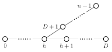
Figure 7: A tree $T_{n,D,h}$.

Lemma 16.

$\lvert\mskip 0.90001muE_{fix}(T_{n,D,h})\mskip 0.90001mu\rvert=\mathbb{F}_{D}\mathbb{F}_{n-D-1}+\mathbb{F}_{h}\mathbb{F}_{D-h}\mathbb{F}_{n-D-2}$.

Proof.

Let $e=(v_{h},v_{D+1})$ and $T_{v_{h}},T_{v_{D+1}}$ the constituents of $T$ for $e$. Then

$$\lvert\mskip 0.90001muE_{fix}(T)\mskip 0.90001mu\rvert=\lvert\mskip 0.90001muE_{fix}(T_{v_{h}},v_{h})\mskip 0.90001mu\rvert\lvert\mskip 0.90001muE_{fix}(T_{v_{D+1}},v_{D+1})\mskip 0.90001mu\rvert+\lvert\mskip 0.90001muE_{fix}(T_{v_{h}})\mskip 0.90001mu\rvert\lvert\mskip 0.90001muE_{fix}(T_{v_{D+1}})\mskip 0.90001mu\rvert$$

by Lemma 4. Clearly, $\lvert\mskip 0.90001muE_{fix}(T_{v_{h}},v_{h})\mskip 0.90001mu\rvert=\mathbb{F}_{h}\mathbb{F}_{D-h}$ and $\lvert\mskip 0.90001muE_{fix}(T_{v_{D+1}},v_{D+1})\mskip 0.90001mu\rvert=\mathbb{F}_{n-D-2}$ by Cor. 5. ∎

The next lemma determines values of $h$ for which $\lvert\mskip 0.90001muE_{fix}(T_{n,D,h})\mskip 0.90001mu\rvert$ is maximal.

Lemma 17.

Let $n,D\in\mathbb{N}$ with $n-2>D\geq 2(n-1)/3$. Let

$$h_{0}=\operatorname*{arg\,max}\limits_{n-D-1\leq h\leq 2D-n+1}\lvert\mskip 0.90001muE_{fix}(T_{n,D,h})\mskip 0.90001mu\rvert.$$

Then $h_{0}=n-D-1$ if $3D=2(n-1)$ and otherwise $h_{0}$ is the first odd integer of $[n-D-1,2D-n+1]$. Furthermore, $\lvert\mskip 0.90001mu{E}_{fix}(T_{n,D,h_{0}})\mskip 0.90001mu\rvert=\mathbb{F}_{D}\mathbb{F}_{n-D-1}+\mathbb{F}_{h_{0}}\mathbb{F}_{D-h_{0}}\mathbb{F}_{n-D-2}$.

Proof.

By Lemma 16 we have $\lvert\mskip 0.90001mu\mathcal{F}_{\mathcal{{M}}}(T_{n,D,h})\mskip 0.90001mu\rvert=\mathbb{F}_{D}\mathbb{F}_{n-D-1}+\mathbb{F}_{h}\mathbb{F}_{D-h}\mathbb{F}_{n-D-2}$. Thus, only the term $\mathbb{F}_{h}\mathbb{F}_{D-h}$ depends on $h$. By Lemma 18 $\mathbb{F}_{h}\mathbb{F}_{D-h}$ it is maximal if $h=h_{0}$. ∎

Lemma 18.

Let $0<x<c$. Then $\mathbb{F}_{x}\mathbb{F}_{c-x}>\mathbb{F}_{x+1}\mathbb{F}_{c-x-1}$ if $x$ is odd and $\mathbb{F}_{x}\mathbb{F}_{c-x}<\mathbb{F}_{x+1}\mathbb{F}_{c-x-1}$ otherwise.

Proof.

The proof is by induction on $x$. Let $x=1$. Then

$$\mathbb{F}_{1}\mathbb{F}_{c-1}=\mathbb{F}_{c-1}>\mathbb{F}_{c-2}=\mathbb{F}_{2}\mathbb{F}_{c-2}.$$

Let $x>1$. Then

$$\mathbb{F}_{x}\mathbb{F}_{c-x} =\mathbb{F}_{x+1}\mathbb{F}_{c-x}-\mathbb{F}_{x-1}\mathbb{F}_{c-x}$$

$$=\mathbb{F}_{x+1}\mathbb{F}_{c-x-1}+\mathbb{F}_{x+1}\mathbb{F}_{c-x-2}-\mathbb{F}_{x-1}\mathbb{F}_{c-x}$$

$$=\mathbb{F}_{x+1}\mathbb{F}_{c-x-1}+\mathbb{F}_{x}\mathbb{F}_{c-x-2}+\mathbb{F}_{x-1}\mathbb{F}_{c-x-2}-\mathbb{F}_{x-1}\mathbb{F}_{c-x}$$

$$=\mathbb{F}_{x+1}\mathbb{F}_{c-x-1}+\mathbb{F}_{x}\mathbb{F}_{c-x-2}-\mathbb{F}_{x-1}\mathbb{F}_{c-x-1}.$$

Now we can apply induction. If $x$ is odd, then $\mathbb{F}_{x-1}\mathbb{F}_{c-x-1}<\mathbb{F}_{x}\mathbb{F}_{c-x-2}$ and hence, $\mathbb{F}_{x}\mathbb{F}_{c-x}>\mathbb{F}_{x+1}\mathbb{F}_{c-x-1}$. Is $x$ is even, then $\mathbb{F}_{x-1}\mathbb{F}_{c-x-1}>\mathbb{F}_{x}\mathbb{F}_{c-x-2}$ and hence, $\mathbb{F}_{x}\mathbb{F}_{c-x}<\mathbb{F}_{x+1}\mathbb{F}_{c-x-1}$. ∎

Let $T_{n,D}$ be a tree that maximizes the number of fixed points among all trees with $n$ nodes and diameter $D$. An interesting question is about the structure of $T_{n,D}$. By an exhaustive search among all trees with $n\leq 34$ using a computer there was just a single case where this was not a star-like tree (all nodes but one have degree $1$ or $2$) that maximizes the number of fixed points (see Fig. 8). We have the following conjecture.

Conjecture 19.

Except for a finite number of cases for each combination of $n$ and $D$ there exists a star-like graph that maximizes the number of fixed points.

Figure 8: A tree with 32 nodes and diameter 7 with 181376 fixed points. All other trees with 32 nodes and diameter 7 have less fixed points.

4.4 Special Cases

Lemma 20.

Let $T$ be a tree with $n\geq 4$ and $\Delta\geq n-\lceil n/3\rceil$ then $\lvert\mskip 0.90001muE_{fix}(T)\mskip 0.90001mu\rvert\leq 2^{n-\Delta-1}$. This bound is sharp.

Proof.

First we construct a tree $T_{m}$ realizing this bound. Let $T_{m}$ be a tree with a single node $v$ with degree $\Delta$, $x=2\Delta-n+1$ neighbors of $v$ are leaves and the remaining $\Delta-x=n-\Delta-1$ neighbors have degree $2$ (see Fig. 6). Assumption $\Delta\geq n-\lceil n/3\rceil$ implies $\Delta-x\leq\Delta/2$. Hence $E_{fix}(T_{m})=\sum_{i=0}^{\Delta-x}\binom{\Delta-x}{i}=2^{\Delta-x}=2^{n-\Delta-1}$ (see also Lemma 9).

Let $v$ be a node of $T$ with degree $\Delta$. Assume that at most two neighbors of $v$ are leaves. Then $n\geq\Delta+1+\Delta-2=2\Delta-1$. This yields $\Delta\leq(n+1)/2$, which contradicts the assumption $\Delta\geq n-\lceil n/3\rceil$. Hence, at least three neighbors of $v$ are leaves. Let $w$ be a non-leaf neighbor of $v$ and $e=(v,w)$. Without loss of generality we can assume that $deg(w)=2$ and that the neighbor $v^{\prime}\not=v$ is a leaf. Next we apply Lemma 4. Let $x$ be a neighbor of $v$ that is a leaf. Note that $E_{fix}(T_{v},u)=E_{fix}(T_{v}\setminus\{w,x\})$. By induction we have $\lvert\mskip 0.90001muE_{fix}(T_{v},u)\mskip 0.90001mu\rvert\leq 2^{n-\Delta-2}$. We also have $\lvert\mskip 0.90001muE_{fix}(T_{v})\mskip 0.90001mu\rvert\leq 2^{n-\Delta-2}$. This yields the upper bound. ∎

Lemma 21.

Let $T$ be a tree with $n-\lceil n/3\rceil>\Delta>(n-1)/2$ then $\lvert\mskip 0.90001muE_{fix}(T)\mskip 0.90001mu\rvert\leq\sum_{i=0}^{\lfloor\Delta/2\rfloor}\binom{n-\Delta-1}{i}$. This bound is sharp.

Proof.

$n-\lceil n/3\rceil>\Delta$ yields $\Delta/2<n/3$ and $\Delta+n/3+1\leq n$. Therefore $\lfloor\Delta/2\rfloor<n-\Delta-1$. Let $U$ be a tree satisfying the assumption and that has the maximal number of fixed points among all such trees. Let $c$ be a node of degree $\Delta$. Assume there exist a neighbor $u$ of $c$ such that the subtree $T_{u}$ rooted in $u$ contains at least three nodes. Since $2\Delta+1>n$, there exists a neighbor $x$ of $c$ that is a leaf. Let $v$ be a leaf of $T_{u}$ and $v_{s}$ its single neighbor such that all neighbors of $v_{s}$ but one are leaves. Let $w$ be this non-leaf neighbor. Assume that $deg(w)>2$. Then there exits a leaf $v^{\prime}\in N(w)$ with $v^{\prime}\not=v$. Detaching node $v^{\prime}$ from $w$ and attaching it to $x$ would increase the number of fixed points. This contradiction shows that $deg(w)=2$.

Assume that $w\not=u$. Le $w_{1}\not=v$ a neighbor of $w$. Using the same argument as above we can assume that $deg(w_{1})=2$. Let $e=(w,w_{1})$. Consider the case with and without $e$. We can apply Lemma 4. This yields

$$\lvert\mskip 0.90001muE_{fix}(T)\mskip 0.90001mu\rvert=\lvert\mskip 0.90001muE_{fix}(T\setminus\{v\})\mskip 0.90001mu\rvert+\lvert\mskip 0.90001muE_{fix}(T\setminus\{v,w\})\mskip 0.90001mu\rvert.$$

Note that both of these trees have maximal degree $\Delta(T)$. Each of these trees either satisfies the assumption of Lemma 21 or Lemma 20. In the former case we can apply induction to get a bound for the number of fixed points. Combining these bound yields the result.

It remains to consider the case $w=u$. Then each neighbor is either a leaf or has a single neighbor that also is a leaf. In this case Lemma 9 yields the result. This type of tree also shows that the bound is sharp. ∎

Let $\tau_{n,\Delta}$ be the maximal value of $\lvert\mskip 0.90001muE_{fix}(T)\mskip 0.90001mu\rvert$ for all trees $T$ with $n$ nodes and maximal degree $\Delta$. We have the following conjecture. If this conjecture is true, it would be possible to determine the structure of all trees with $\lvert\mskip 0.90001muE_{fix}(T)\mskip 0.90001mu\rvert=\tau_{n,\Delta}$.

Conjecture 22.

$\tau_{n,\Delta}=\tau_{n-1,\Delta}+\tau_{n-2,\Delta}$ for $\Delta<(n-1)/2$.

5 Pure 2-Cycles

In this section we prove an upper bound for $\lvert\mskip 0.90001mu\mathcal{P}_{\mathcal{M}}(T)\mskip 0.90001mu\rvert$. Again we use the fact that $\lvert\mskip 0.90001mu\mathcal{P}_{\mathcal{M}}(T)\mskip 0.90001mu\rvert=2\lvert\mskip 0.90001muE_{pure}(T)\mskip 0.90001mu\rvert$ [23]. Note that Algorithm 1 can be easily adopted to compute $\lvert\mskip 0.90001muE_{pure}(T)\mskip 0.90001mu\rvert$. The difference between $\mathcal{F}$-legal and $\mathcal{P}$-legal is that instead of $2deg_{F}(v)\leq deg(v)$ condition $2deg_{F}(v)<deg(v)$ is required. If $deg(v)$ is odd then the conditions are equivalent. Thus, it suffices to define for each node $v_{i}$ with even degree $b_{i}=\lfloor deg(v_{i})/2\rfloor-1$. Hence, $\lvert\mskip 0.90001muE_{pure}(T)\mskip 0.90001mu\rvert$ can be computed in time $O(n\Delta)$.

Note that $E_{pure}(T)\subseteq E_{fix}(T)$ with $E_{pure}(T)=E_{fix}(T)$ if all degrees of $T$ are odd. Thus, $\lvert\mskip 0.90001muE_{pure}(T)\mskip 0.90001mu\rvert\leq F_{n-\lceil\Delta/2\rceil}$. In this section we prove the much better general upper bound stated in Theorem 3. We start with an example. Let $n\equiv 0(2)$ and $H_{n}$ the tree with $n$ nodes consisting of a path $P_{n}$ of length $n/2$ and a single node attached to each inner node of $P_{n}$ (see Fig. 9). Since all non-leaves have degree $3$ we have $E_{pure}(H_{n})=E_{fix}(P_{n})$, thus, $\lvert\mskip 0.90001muE_{pure}(H_{n})\mskip 0.90001mu\rvert\leq F_{n/2}$ by Corollary 5. We prove that $F_{\lfloor n/2\rfloor}$ is an upper bound for $\lvert\mskip 0.90001muE_{pure}(T)\mskip 0.90001mu\rvert$ in general.

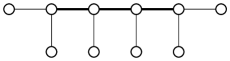
Figure 9: The graph $H_{10}$, edges of $E^{3}(H_{10})$ are depicted as solid lines.

We first state a few technical lemmas and then prove Theorem 3. The proof of the first Lemma is similar to Lemma 12.

Lemma 23.

Let $T$ be a tree, $v$ a leaf with neighbor $w$, and $T^{\prime}=T\setminus v$. Let $n_{l}$ (resp. $n_{i}$) be the number of neighbors of $w$ that are leaves (resp. inner nodes). If $n_{l}>n_{i}+1$ then $\lvert\mskip 0.90001muE_{pure}(T)\mskip 0.90001mu\rvert=\lvert\mskip 0.90001muE_{pure}(T^{\prime})\mskip 0.90001mu\rvert$.

For a tree $T$ let $T^{2}$ be the tree obtained from $T$ by recursively removing each node $v$ with degree $2$ and connecting the two neighbors of $v$ by a new edge. Note that $T^{2}$ is uniquely defined and $deg_{T^{2}}(v)=deg_{T}(v)$ for each node $v$ of $T^{2}$. The next lemma is easy to prove.

Lemma 24.

$E_{pure}(T)\subseteq E_{pure}(T^{2})$ for each tree $T$.

Proof.

Let $w$ be a node $v$ of $T$ with degree $2$. Let $T^{\prime}$ be the tree obtained from $T$ by removing $w$ and connecting the two neighbors of $w$ by a new edge. Let $F\in E_{pure}(T)$. Since $deg(w)=2$ no edge of $F$ is incident to $w$. Thus, for all $v\not=w$ we have $2deg_{F}(v)<deg_{T}(v)=deg_{T^{\prime}}(v)$, i.e., $F\in E_{pure}(T^{\prime})$. Hence, $E_{pure}(T)\subseteq E_{pure}(T^{\prime})$ and the statement follows by induction. ∎

Proof of Theorem 3.

Proof by induction on $n$. The statement is true for $n\leq 5$ as can be seen by a simple inspection of all cases. Let $n\geq 6$. By Lemma 24 we can assume that no node of $T$ has degree $2$. Let $\hat{T}$ be the tree induced by the edges in $E^{3}(T)$. $\hat{T}$ includes all inner nodes of $T$. Let $u$ be a node of $\hat{T}$ such that all neighbors of $u$ in $\hat{T}$ except one are leaves. Denote the neighbors of $u$ in $\hat{T}$ that are leaves by $v_{1},\ldots,v_{d}$ with $d\geq 1$, i.e., $deg_{\hat{T}}(u)=d+1$. Let $e_{i}=(u,v_{i})$. By Lemma 23 we can assume $deg_{T}(v_{i})=3$ for $i=1,\ldots,d$. Denote the two neighbors of $v_{i}$ in $T\setminus\hat{T}$ by $v_{i}^{a}$ and $v_{i}^{b}$. Let $H_{1}=\{F\in E_{pure}(T)\;|\;e_{1}\not\in F\}$ and $T^{\prime}=T\setminus\{v_{1}^{a},v_{2}^{b}\}$. Clearly $H_{1}=E_{pure}(T^{\prime})$. Thus, $\lvert\mskip 0.90001muH_{1}\mskip 0.90001mu\rvert\leq\mathbb{F}_{\lfloor n/2\rfloor-1}$ by induction. Assume that $u$ has a neighbor $u^{\prime}$ in $T$ that is a leaf in $T$. Let $F\in E_{pure}(T)\setminus H_{1}$. Then $F\setminus\{e_{1}\}\in E_{pure}(T\setminus\{u^{\prime},v_{1},v_{1}^{a},v_{1}^{b}\})$. Thus, by induction $\lvert\mskip 0.90001muE_{pure}(T)\setminus H_{1}\mskip 0.90001mu\rvert\leq\mathbb{F}_{\lfloor n/2\rfloor-2}$ and hence, $\lvert\mskip 0.90001muE_{pure}(T)\mskip 0.90001mu\rvert\leq\mathbb{F}_{\lfloor n/2\rfloor}$. Therefore we can assume that $deg_{T}(u)=d+1$, i.e., $d\geq 2$.

Next we expand the definition of $H_{1}$ as follows. For $i=1,\ldots,d$ let

$$H_{i}=\{F\in E_{pure}(T)\;|\;e_{i}\not\in F\text{ and }e_{1},\ldots,e_{i-1}\in F\}.$$

Thus, $H_{i}=\emptyset$ for $i\geq(d+3)/2$ since $2deg_{F}(u)<d+1$. Let $d_{0}=\lfloor(d+1)/2\rfloor$. Then $E_{pure}(T)=H_{1}\cup\ldots\cup H_{d_{o}}$. We claim that $\lvert\mskip 0.90001muH_{i}\mskip 0.90001mu\rvert\leq\mathbb{F}_{\lfloor n/2\rfloor-(2i-1)}$. The case $i=1$ was already proved above. Let $i\geq 2$ and define $T_{i}=T\setminus\{v_{j},v_{j}^{a},v_{j}^{b}\;|\;j=i-1,i\}$. Then $\lvert\mskip 0.90001muE_{pure}(T_{i})\mskip 0.90001mu\rvert\leq\mathbb{F}_{\lfloor n/2\rfloor-3}$ by induction, hence $\lvert\mskip 0.90001muH_{2}\mskip 0.90001mu\rvert=\lvert\mskip 0.90001muE_{pure}(T_{2})\mskip 0.90001mu\rvert\leq\mathbb{F}_{\lfloor n/2\rfloor-3}$. Let $i\geq 3$ and $F\in H_{i}$. Then $F\setminus\{e_{i-1}\}\in E_{pure}(T_{i})$. Clearly, $E_{pure}(T_{i})\setminus H_{i}$ consists of all $F\in E_{pure}(T_{i})$ for which $\{e_{1},\ldots,e_{i-2}\}\cap F\not=\emptyset$ holds. Hence,

$$\lvert\mskip 0.90001muH_{i}\mskip 0.90001mu\rvert\leq\lvert\mskip 0.90001muE_{pure}(T_{i})\mskip 0.90001mu\rvert-\lvert\mskip 0.90001mu\bigcup_{j=1}^{i-2}E_{j}^{i}\mskip 0.90001mu\rvert\leq\mathbb{F}_{\lfloor n/2\rfloor-3}-\lvert\mskip 0.90001mu\bigcup_{j=1}^{i-2}E_{j}^{i}\mskip 0.90001mu\rvert$$

where $E_{j}^{i}=\{F\in E_{pure}(T_{i})\;|\;e_{j}\not\in F\}$. We use the following well known identity for $I=\{1,\ldots,i-2\}$.

$$\lvert\mskip 0.90001mu\bigcup_{i\in I}E_{i}\mskip 0.90001mu\rvert=\sum_{\emptyset\not=J\subseteq I}(-1)^{\lvert\mskip 0.90001muJ\mskip 0.90001mu\rvert+1}\lvert\mskip 0.90001mu\bigcap_{j\in J}E_{i}\mskip 0.90001mu\rvert$$

Note that $\lvert\mskip 0.90001mu\bigcap_{j\in J}E_{j}^{i}\mskip 0.90001mu\rvert\leq\mathbb{F}_{\lfloor n/2\rfloor-(\lvert\mskip 0.90001muJ\mskip 0.90001mu\rvert+3)}$ by induction. Let $k=i-2$. Then

$$\lvert\mskip 0.90001muH_{i}\mskip 0.90001mu\rvert\leq\mathbb{F}_{\lfloor n/2\rfloor-3}-\sum_{j=1}^{k}(-1)^{j+1}\binom{k}{j}\mathbb{F}_{\lfloor n/2\rfloor-(j+3)}=\sum_{j=0}^{k}(-1)^{j}\binom{k}{j}\mathbb{F}_{\lfloor n/2\rfloor-(j+3)}$$

Note that $\lfloor n/2\rfloor\geq 2k+3$. Lemma 25 implies $\lvert\mskip 0.90001muH_{i}\mskip 0.90001mu\rvert\leq\mathbb{F}_{\lfloor n/2\rfloor-(2i-1)}$. Then Lemma 26 yields

$$\lvert\mskip 0.90001muE_{pure}(T)\mskip 0.90001mu\rvert\leq\sum_{i=1}^{d_{0}}\lvert\mskip 0.90001muH_{i}\mskip 0.90001mu\rvert\leq\sum_{i=1}^{d_{0}}\mathbb{F}_{\lfloor n/2\rfloor-(2i-1)}\leq\mathbb{F}_{\lfloor n/2\rfloor}.$$

∎

Lemma 25.

For each $k\geq 0$ and $c\geq 2k+3$ we have

$$\mathbb{F}_{c-(2k+3)}=\sum_{i=0}^{k}(-1)^{i}\binom{k}{i}\mathbb{F}_{c-(i+3)}.$$

Proof.

The proof is by induction on $k$. The cases $k\leq 2$ clearly hold. Let $k>2$.

$$\sum_{i=0}^{k}(-1)^{i}\binom{k}{i}\mathbb{F}_{c-(i+3)}$$

$$\leavevmode\nobreak\ =(-1)^{k}\mathbb{F}_{c-(k+3)}+\sum_{i=0}^{k-1}(-1)^{i}\binom{k}{i}\mathbb{F}_{c-(i+3)}$$

$$\leavevmode\nobreak\ =(-1)^{k}\mathbb{F}_{c-(k+3)}+\sum_{i=0}^{k-1}(-1)^{i}\binom{k-1}{i}\mathbb{F}_{c-(i+3)}+\sum_{i=1}^{k-1}(-1)^{i}\binom{k-1}{i-1}\mathbb{F}_{c-(i+3)}$$

$$\stackrel{{\scriptstyle\text{Ind.}}}{{=}}(-1)^{k}\mathbb{F}_{c-(k+3)}+\mathbb{F}_{c-(2k+1)}-\sum_{i=0}^{k-2}(-1)^{i}\binom{k-1}{i}\mathbb{F}_{c-(i+4)}$$

$$\leavevmode\nobreak\ =(-1)^{k}\mathbb{F}_{c-(k+3)}+\mathbb{F}_{c-(2k+1)}-\sum_{i=0}^{k-1}(-1)^{i}\binom{k-1}{i}\mathbb{F}_{c-1-(i+3)}+(-1)^{k-1}\mathbb{F}_{c-(k+3)}$$

$$\stackrel{{\scriptstyle\text{Ind.}}}{{=}}\mathbb{F}_{c-(2k+1)}-\mathbb{F}_{c-1-(2k+1)}$$

$$\leavevmode\nobreak\ =\mathbb{F}_{c-(2k+3)}$$

∎

Lemma 26.

For each $c\geq 1$ and $d\leq\frac{c+1}{2}$ we have $\sum_{i=1}^{d}\mathbb{F}_{c-(2i-1)}\leq\mathbb{F}_{c}$.

Proof.

The proof is by induction on $d$. The cases $d\leq 2$ clearly hold. Let $d>2$. By induction we get

$$\sum_{i=1}^{d}\mathbb{F}_{c-(2i-1)}=\mathbb{F}_{c-1}+\sum_{i=2}^{d}\mathbb{F}_{c-(2i-1)}=\mathbb{F}_{c-1}+\sum_{i=1}^{d-1}\mathbb{F}_{c-2-(2i-1)}\stackrel{{\scriptstyle\text{Ind.}}}{{\leq}}\mathbb{F}_{c-1}+\mathbb{F}_{c-2}=\mathbb{F}_{c}.$$

∎

5.1 Special Cases

Lemma 27.

Let $T$ a tree with $n$ nodes and diameter $D$ such that $2D\geq n$. Then $\lvert\mskip 0.90001muE_{pure}(T)\mskip 0.90001mu\rvert\leq\mathbb{F}_{n-D}$ and this bound is sharp.

Proof.

Let $P$ be a path of length $D$ of $T$. Thus, at most $n-(D+1)$ nodes can have degree $3$. Each such node can be associated with a unique node of degree $1$. Thus, at most $n-(D+1)$ neighboring nodes on $P$ have degree 3. This leads to $n-D$ adjacent edges from $E^{3}(T)$ and hence, $\lvert\mskip 0.90001muE_{pure}(T)\mskip 0.90001mu\rvert\leq\mathbb{F}_{n-D}$. The trees $H_{n}$ (see Fig. 9) prove that the bound is sharp. ∎

If $n>2D$ this bound does not hold. It is easy to see that for $n=2D+1$ the maximal number of fixed points is $\mathbb{F}_{n-(D+1)}$ (see Fig. 10).

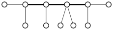
Figure 10: The graph $H_{10}$ with an additional node has 10 pure 2-cycles.

Lemma 28.

Let $n<2\Delta+1$ and $T$ a tree with $n$ nodes and maximal degree $\Delta$. Then $\lvert\mskip 0.90001muE_{pure}(T)\mskip 0.90001mu\rvert\leq 2^{\lfloor\frac{n-\Delta-1}{2}\rfloor}$. This bound is sharp.

Proof.

Let $x\leq\Delta$ such that $2(\Delta-x)<\Delta$. Let $v$ be a node of degree $\Delta$ that has $x$ leaves as neighbors and the remaining $\Delta-x$ neighbors have degree $3$, i.e., $x=(1+3\Delta-n)/2$. Then clearly $\lvert\mskip 0.90001muE_{pure}(T)\mskip 0.90001mu\rvert=2^{\Delta-x}$. Note that $\Delta-x=(n-\Delta-1)/2$. ∎

For a tree $T$ let $\delta_{T}$ be the smallest degree of an inner node of $T$ with degree at least $3$, i.e., $\delta_{T}=\min\{deg(v)\;|\;v\in V\text{ with }deg(v)>2\}$.

Lemma 29.

Let $T$ be a tree with $\Delta>2$ and $n^{\prime}$ the number of nodes of $T^{2}$. Then $\lvert\mskip 0.90001muE_{pure}(T)\mskip 0.90001mu\rvert\leq 2^{(n^{\prime}-2)/(\delta_{T}-1)-1}$.

Proof.

The proof is by induction on $t$, the number of nodes of $T$ with degree $2$. Let $t=0$, then $n=n^{\prime}$. Denote the number of leaves (resp. inner nodes) by $l$ (resp. $i$). Then clearly $l\geq(\delta_{T}-2)i+2$ and $i\leq(n-2)/(\delta_{T}-1)$. This yields

$$\lvert\mskip 0.90001muE^{3}(T)\mskip 0.90001mu\rvert=n-1-l=i-1\leq(n-2)/(\delta_{T}-1)-1.$$

Therefore, $\lvert\mskip 0.90001muE_{pure}(T)\mskip 0.90001mu\rvert\leq 2^{(n-2)/(\delta_{T}-1)-1}$. Assume $t>0$ and let $w$ be a node of $T$ with $deg(w)=2$. Let $T^{\prime}$ be the tree obtained from $T$ by removing $w$ and connecting the two neighbors of $w$ by a new edge. Then $(T^{\prime})^{2}=T^{2}$ and $\delta_{T^{\prime}}=\delta_{T}$. By induction $\lvert\mskip 0.90001muE_{pure}(T^{\prime})\mskip 0.90001mu\rvert\leq 2^{(n^{\prime}-2)/(\delta_{T}-1)-1}$. Since $\lvert\mskip 0.90001muE_{pure}(T)\mskip 0.90001mu\rvert\leq\lvert\mskip 0.90001muE_{pure}(T^{\prime})\mskip 0.90001mu\rvert$ (see Lemma 24) the proof is complete. ∎

For $\delta_{T}\geq 4$ we have $\mathbb{F}_{n/2}>2^{(n-2)/(\delta_{T}-1)-1}$, i.e., a better bound than that provided in Theorem 3. If $\delta_{T}=3$ the other bound is lower since $\mathbb{F}_{n/2}\leq 2^{n/2-2}$.

6 Conclusion and Open Problems

The problem of counting the fixed points for general cellular automata is #P-complete. In this paper we considered counting problems associated with the minority/majority rule of tree cellular automata. In particular we examined fixed points and pure 2-cycles. The first contribution is a novel algorithm that counts the fixed points and the pure 2-cycles of such an automata. The algorithms run in time $O(\Delta n)$. It utilizes a characterization of colorings for these automata in terms of subsets of the tree edges. This relieved us from separately treating the minority and the majority rule. The second contribution are upper and lower bounds for the number of fixed points and pure 2-cycles based on different graph parameters. We also provided examples to demonstrate the cases when these bounds are sharp. The bounds show that the number of fixed points (resp. 2-cycles) is a tiny fraction of all colorings.

There are several open questions that are worth pursuing. Firstly, we believe that it is possible to sharpen the provided bounds and to construct examples for these bounds. In particular for the case $\Delta\leq n/2$, we believe that our bounds can be improved. Another line of research is to extend the analysis to generalized classes of minority/majority rules. One option is to consider the minority/majority not just in the immediate neighborhood of a node but in the r-hop neighborhood for $r>1$ [16]. We believe that this complicates the counting problems considerably.

Finally the predecessor existence problem and the corresponding counting problem [7] have not been considered for tree cellular automata. The challenge is to find for a given $c\in\mathcal{C}(T)$ a coloring $c^{\prime}\in\mathcal{C}(T)$ with $\mathcal{M}(c^{\prime})=c$. A coloring $c\in\mathcal{C}(T)$ is called a garden of Eden coloring if there doesn’t exist a $c^{\prime}\in\mathcal{C}(T)$ with $\mathcal{M}(c^{\prime})=c$. The corresponding counting problem for tree cellular automata is yet unsolved.

Appendix A Execution of Algorithm 1

In this appendix we give an example for the execution of Algorithm 1. We use the tree of Fig. 4 which is for convenience shown again in Fig. 11.

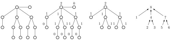
Figure 11: From left to right: Tree $T$, annotation of $T$, $T_{R}$, a postorder numbering of $T_{R}$.

For the tree in Fig. 11 we have

$$w(T_{7},2) =w(T_{4},2)w(S_{7},1)+w(T_{4},1)w(S_{7},0)=w(T_{4},2)w(T_{6},1)+w(T_{4},1)w(T_{6},0)$$

$$w(T_{4},2) =w(T_{1},2)w(S_{4},1)+w(T_{1},1)w(S_{4},0)=w(T_{1},2)w(T_{3},1)+w(T_{1},1)w(T_{3},0)$$

$$w(T_{1},2) =w(S_{1},1)+w(S_{1},0)=2$$

$$w(T_{3},1) =w(T_{2},1)w(S_{3},1)+w(T_{2},0)w(S_{3},0)=w(T_{2},1)+w(T_{2},0)$$

$$w(T_{2},1) =w(S_{2},1)+w(S_{2},0)=1+1=2$$

$$w(T_{2},0) =w(S_{2},1)=1$$

$$w(T_{3},1) =3$$

$$w(T_{1},1) =w(S_{1},1)+w(S_{1},0)=2$$

$$w(T_{3},0) =w(T_{2},0)w(S_{3},1)+w(T_{2},-1)w(S_{3},0)=1$$

$$w(T_{4},1) =w(T_{1},1)w(S_{4},1)+w(T_{1},0)w(S_{4},0)=w(T_{1},1)w(T_{3},1)+w(T_{1},0)w(T_{3},0)=2*3+1*1=7$$

Hence, $w(T_{4},2)=8$, $w(T_{7},2)=31$, and therefore $\lvert\mskip 0.90001mu\mathcal{F}_{\mathcal{M}}(T)\mskip 0.90001mu\rvert=62$. The complete array $W$ is as follows.

$T_{k}$	$0$	$1$	$2$	$3$	$4$	$5$	$6$	$7$
$b=0$	$1$	1	1	1	3	1	1	9
$b=1$	$1$	2	2	3	7	2	3	24
$b=2$	$1$	2	2	3	8	2	3	31

References

- [1] Agur, Z.: Fixed points of majority rule cellular automata with application to plasticity and precision of the immune system. Complex Systems 5(3), 351–357 (1991)
- [2] Agur, Z., Fraenkel, A., Klein, S.: The number of fixed points of the majority rule. Discrete Mathematics 70(3), 295–302 (1988). https://doi.org/10.1016/0012-365X(88)90005-2
- [3] Akutsu, T., Kuhara, S., Maruyama, O., Miyano, S.: A system for identifying genetic networks from gene expression patterns produced by gene disruptions and overexpressions. Genome Informatics 9, 151–160 (1998)
- [4] Aledo, J.A., Diaz, L.G., Martinez, S., Valverde, J.C.: Enumerating periodic orbits in sequential dynamical systems over graphs. Journal of Computational and Applied Mathematics 405, 113084 (2022). https://doi.org/10.1016/j.cam.2020.113084
- [5] Aracena, J.: Maximum number of fixed points in regulatory boolean networks. Bulletin of mathematical biology 70(5), 1398 (2008)
- [6] Aracena, J., Richard, A., Salinas, L.: Maximum number of fixed points in and–or–not networks. J. of Computer & System Sciences 80(7), 1175–1190 (2014). https://doi.org/10.1016/j.jcss.2014.04.025
- [7] Barrett, C., Hunt III, H.B., Marathe, M.V., Ravi, S., Rosenkrantz, D.J., Stearns, R.E., Thakur, M.: Predecessor existence problems for finite discrete dynamical systems. Theoretical Computer Science 386(1-2), 3–37 (2007)
- [8] Bridoux, F., Durbec, A., Perrot, K., Richard, A.: Complexity of fixed point counting problems in boolean networks. J. Comput. Syst. Sci. 126, 138–164 (2022). https://doi.org/10.1016/j.jcss.2022.01.004
- [9] Fogelman, F., Goles, E., Weisbuch, G.: Transient length in sequential iteration of threshold functions. Discrete Applied Mathematics 6(1), 95–98 (1983)
- [10] Goles, E., Olivos, J.: Periodic behaviour of generalized threshold functions. Discrete Mathematics 30(2), 187 – 189 (1980). https://doi.org/10.1016/0012-365X(80)90121-1
- [11] Irons, D.: Improving the efficiency of attractor cycle identification in boolean networks. Physica D: Nonlinear Phenomena 217(1), 7–21 (2006). https://doi.org/10.1016/j.physd.2006.03.006
- [12] Kauffman, S., et al.: The origins of order: Self-organization and selection in evolution. Oxford University Press, USA (1993)
- [13] Královič, R.: On majority voting games in trees. In: SOFSEM: Theory and Practice of Informatics. pp. 282–291. Springer (2001)
- [14] Mezzini, M., Pelayo, F.L.: An algorithm for counting the fixed point orbits of an and-or dynamical system with symmetric positive dependency graph. Mathematics 8(9), 1611 (2020)
- [15] Mishra, S., Rao, S.: Minimum monopoly in regular and tree graphs. Discrete Mathematics 306(14), 1586–1594 (2006). https://doi.org/10.1016/j.disc.2005.06.036
- [16] Moran, G.: The r-majority vote action on 0–1 sequences. Discr. Math. 132(1-3), 145–174 (1994)
- [17] Nakar, Y., Ron, D.: The structure of configurations in one-dimensional majority cellular automata: From cell stability to configuration periodicity. In: 15th Int. Conf. on Cellular Automata. LNCS, vol. 13402, pp. 63–72. Springer (2022). https://doi.org/10.1007/978-3-031-14926-9_6
- [18] Papp, P., Wattenhofer, R.: Stabilization Time in Minority Processes. In: 30th Int. Symp. on Algorithms & Computation. LIPIcs, vol. 149, pp. 43:1–43:19 (2019). https://doi.org/10.4230/LIPIcs.ISAAC.2019.43
- [19] Peleg, D.: Local majorities, coalitions and monopolies in graphs: a review. Theoretical Computer Science 282(2), 231–257 (2002)
- [20] Poljak, S., Sura, M.: On periodical behaviour in societies with symmetric influences. Combinatorica 3(1), 119–121 (1983)
- [21] Rouquier, J., Regnault, D., Thierry, E.: Stochastic minority on graphs. Theoretical Computer Science 412(30), 3947–3963 (2011). https://doi.org/10.1016/j.tcs.2011.02.028
- [22] Tošić, P., Agha, G.: On computational complexity of counting fixed points in symmetric boolean graph automata. In: Unconventional Computation. pp. 191–205. Springer (2005)
- [23] Turau, V.: Fixed points and 2-cycles of synchronous dynamic coloring processes on trees. In: 29th Int. Coll. on Structural Information and Communication Complexity - Sirocco. pp. 265–282. Springer (Jun 2022)
- [24] Veliz-Cuba, A., Laubenbacher, R.: On the computation of fixed points in boolean networks. Journal of Applied Mathematics and Computing 39, 145–153 (2012). https://doi.org/10.1007/s12190-011-0517-9
- [25] Zehmakan, A.: On the Spread of Information Through Graphs. Ph.D. thesis, ETH Zürich (2019)