Automated Market Maker on the XRP Ledger

Abstract

This research paper focuses on the testing and evaluation of the proposed xrpl-amm, designed to address the limitations observed in traditional Ethereum-based amms, such as high transaction fees, significant slippage, high impermanent losses, synchronization issues, and low transaction throughput. xrpl-amm leverages the swift, cost-efficient transaction capabilities of xrpl and its unique design, featuring a cam that encourages arbitrage transactions for more efficient price synchronization with external markets.

Our testing and evaluation of the proposed xrpl-amm compares its performance against established players like Uniswap. Our evaluation results reveal that the xrpl-amm, leveraging market volatility, outperforms Uniswap in various areas, including slippage and impermanent loss reduction, the pace of price synchronization, and overall operational efficiency.

Our research contributes to the growing field of defi by providing comprehensive testing results that underline xrpl-amm’s potential as a more efficient alternative to current amms while encouraging further exploration in xrpl-based defi ecosystems.

I Introduction

Decentralized Finance (defi) has revolutionized the financial sector by leveraging blockchain technology to offer alternative, transparent financial services, eliminating the need for traditional intermediaries like banks [1]. defi, enabled by smart contracts on platforms such as Ethereum, encompasses a variety of services, ranging from lending to asset management [2, 3, 4]. It is characterized by its ability to reduce intermediary costs and democratize financial access, earning the nickname ”financial lego” due to its modular nature that facilitates the creation of complex financial products [2]. This innovation suggests a potential reshaping of the financial landscape.

A pivotal aspect of defi is the Automated Market Maker (amm), a novel dex protocol introduced by Bancor in 2017 and later popularized by Uniswap in 2018 [5, 6]. amms use algorithms for asset pricing to facilitate trading and liquidity creation, eliminating the need for traditional market participants. amms have become instrumental in providing liquidity for less popular assets [5, 6, 7, 8].

Despite their utility, most amms operate on the Ethereum blockchain and face challenges such as high transaction fees, significant slippage, impermanent loss risks, and synchronization issues [9, 10]. To address these concerns, this paper investigates the performance of an amm integrated at the protocol level of the XRP Ledger (xrpl), known for its rapid and low-cost transactions. We aim to demonstrate that the xrpl-amm surpasses traditional Ethereum-based amms like Uniswap regarding speed, scalability, and efficiency [11].

Our research compares the xrpl-amm with Uniswap, chosen for its dominance of over 60% in dexs market share by trading volume [12]. Our results show that the xrpl-amm reduces slippage and impermanent losses, improves price synchronization speed, and enhances overall operational efficiency.

II Related Work

Significant research has focused on various amms, yielding diverse models and approaches. Key studies, such as [10, 13, 14], offer insights into major amms’ features, crucial for comparing with the xrpl-amm. Notably, Uniswap V2 minimizes gas fees with a simple bonding curve, V3 improves capital efficiency via concentrated liquidity, Balancer supports multi-asset pools, Curve.fi specializes in similar-pegged assets, and DODO integrates external price feeds to counteract divergence loss [10]. Despite these differences, most amms, including these, are based on or adapted from Uniswap V2’s cpmm model [10, 15].

On the other hand, existing amm research predominantly focuses on Ethereum-based dexs [10], which are mostly built as smart contracts executing on top of a blockchain via, most of the time, the Ethereum Virtual Machine (EVM). This architecture often lags in transaction execution speed compared to native transactions, leading to increased slippage. Additionally, to the best of our knowledge, there are no other amms built directly at the protocol level of a blockchain, making direct comparisons with the xrpl-amm challenging. Moreover, considering the lack of existing research on xrpl-based amm solutions, this inaugural study ventures into the unexplored domain of xrpl-based amms and highlights the advantages of protocol-level integration compared to traditional smart contracts implementations, noting the challenges of direct comparison.

III Backgroud & Terminology

Table I provides a brief overview of amm-based dexs. Additionally, we include in Table II a glossary of terms used in this paper.

TABLE I: Background on AMM-Based DEX

Overview
AMM-Based DEX: amms play a crucial role in the DeFi ecosystem, facilitating asset exchanges and liquidity management. Unlike traditional exchanges that rely on order books, amms use algorithms for asset pricing. Despite the varying mechanics across protocols, all amms use a conservation function (or bonding curve) to maintain pool asset balances.
AMM Participants: amms have two primary agents: exchange users, who swap assets, and liquidity providers, who supply liquidity and earn trading fees. A subgroup of exchange users, arbitrageurs, exploits price discrepancies between amms and external markets to ensure amm price alignment.
AMM Implicit Economic Costs: amms, despite their advancements, have inherent risks. Users and providers face economic challenges, notably slippage and impermanent loss (or divergence loss). Slippage refers to the price difference between when a trade is initiated and executed. Impermanent loss is the potential opportunity cost for liquidity providers due to price shifts of supplied assets in amms.

TABLE II: Terms used in this paper and their descriptions.

Term
$\Gamma_{X}$: Current balance of token $X$ in the amm instance pool
$\Gamma_{LPTokens}$: Current LPTokens outstanding balance issued by the amm instance
$\Delta{{}_{X}}^{+}$: Amount of asset $X$ being added to the amm instance pool
$\Delta{{}_{X}}^{-}$: Amount of asset $X$ being removed from the amm instance pool
${\it TFee}$: Trading fee (up to 1%) of the amm instance, charged on the portion of the trade that changes the ratio of tokens in a pool
$W_{X}$: Normalized weight of token $X$ in the amm instance pool
Arbitrageurs: Exchange users who profit from price discrepancies between amms and external markets.
lps: Traders managing pool liquidity. They receive trading fees and are issued LPTokens upon providing liquidity.
LPTokens: Represent lps shares of the amm pool. Can be transferred. They are reward mechanism to help facilitate transactions between different types of currencies.
Spot-Exchange Rate (SPE): Weighted ratio of the instance’s pool balances: $SPE_{A}^{B}=\frac{\frac{\Gamma_{B}}{W_{B}}}{\frac{\Gamma_{A}}{W_{A}}}\cdot\frac{1}{1-{\it TFee}}$
Effective Price (EP): Ratio of swapped in (Token B) to swap out (Token A) tokens: $EP_{A}^{B}=\frac{\Delta_{B}^{+}}{\Delta_{A}^{-}}$
Slippage: Change in effective price relative to pre-swap rate: $Slippage=\frac{EP_{A}^{B}}{{}_{pre-swap}SPE_{A}^{B}}-1$
Price Impact: Change in spot exchange rate caused by a swap: $PriceImpact=\frac{{}_{post-swap}SPE_{A}^{B}}{{}_{pre-swap}SPE_{A}^{B}}-1$

IV Underlying Infrastructure

The xrpl-amm is powered by the xrpl, which has been operating, conceivably, the world’s oldest dex [16]. This platform has provided liquidity through manual market making and order books for over a decade. Some properties of the xrpl that benefit the amm-based dex are:

• Federated Consensus & ctor: Transactions in the xrpl follow a canonical order based on their transaction hash, ensuring standardization. Unlike blockchains where nodes individually race to solve a puzzle for rewards [17], ctor promotes collaboration. Every node works together, following instructions to agree on a transaction sequence. Unlike other networks susceptible to transaction order manipulation, XRPL’s use of CTOR obfuscates transaction sequencing. This diminishes the potential for Miner Extractable Value (MEV) and tactics like front-running or sandwich attacks that can deter traders [18], though they remain feasible [19].

• Fast finality: The xrpl confirms a new ledger roughly every four seconds [20], faster than most other blockchains like Ethereum, which takes about 12 seconds [21].

• Pathfinding: xrpl’s amm-based dex interacts with xrpl’s limit order book (LOB) based dex. The pathfinding method identifies whether swapping within a liquidity pool or through the order book will provide the best exchange rate.

• Low network transaction fee: The minimum transaction cost required by the xrpl network for a standard transaction is 0.00001 XRP (10 drops) [22]. Due to the remarkably low network fees on xrpl, users can operate without concern over transaction fees.

• Protocol native: The protocol-level implementation of the amm-based dex establishes it as an integral element of the xrpl. A singular amm instance per asset pair is permissible. Within the xrpl, two tokens can share the same currency code while being issued by different entities. This allows for separate amm instances with identical currency pairs, like USD_issuer1/USD_issuer2, analogous to Ethereum’s ETH/WETH or USDT/USDC pools. The same currency can also pair with the same asset in distinct amm instances, leading to opportunities for arbitrageurs both within and outside the amm-based dex, enhancing price discovery. For instance, a pool with XRP/USD_issuer1 differs from a pool with XRP/USD_issuer2. While XRP is the native cryptocurrency of the xrpl and not an IOU token, other tokens are identified by currency codes and come with specific standards [23]. LPTokens, although not IOU tokens, cannot initiate new amm instances [11].

V xrpl amm Design

This section highlights key aspects of the XRPL-AMM’s design. For a comprehensive exploration, including topics such as conservation function, (pure and single-sided) liquidity provision and withdrawal, and votable trading fee governance, refer to the original proposition of the XRPL AMM [11].

V-A Swap

Let B be the asset being swapped into the pool and A the asset being swapped out, then:

if the user specifies the amount of B to swap in:

$$\scriptsize\Delta_{A}^{-}=\Gamma_{A}\cdot\left[1-\left(\frac{\Gamma_{B}}{\Gamma_{B}+\Delta_{B}^{+}\cdot\left(1-{\it TFee}\right)}\right)^{\frac{W_{B}}{W_{A}}}\right]$$ (1)

and if the user specifies the amount of A to swap out:

$$\scriptsize\Delta_{B}^{+}=\Gamma_{B}\left[\left(\frac{\Gamma_{A}}{\Gamma_{A}-\Delta_{A}^{-}}\right)^{\frac{W_{A}}{W_{B}}}-1\right]\cdot\frac{1}{1-{\it TFee}}$$ (2)

with $W_{A}=W_{B}=0.5$.

In addition, to change the spot-exchange rate of asset A traded out from $SPE_{A}^{B}$ to $SPE_{A}^{{}^{\prime}B}$, the user needs to swap in:

$$\scriptsize\Delta_{B}^{+}=\Gamma_{B}\cdot\left[\left(\frac{SPE_{A}^{{}^{\prime}B}}{SPE_{A}^{B}}\right)^{\left(\frac{W_{A}}{W_{A}+W_{B}}\right)}-1\right]$$ (3)

Equation 1 then computes the received amount of token A.

V-B Continuous Auction Mechanism (CAM)

The cam permits LPToken holders to bid for a daily slot offering a 0% trading fee, attracting arbitrageurs, while other users maintain normal pool access. Winners secure the slot for at least one ledger cycle (roughly 4 seconds) and retain it until outbid or the 24-hour period ends.

V-B1 Mechanics

The auction slot’s bid price changes dynamically. As the slot’s duration progresses, its price decreases. A higher bid (per unit time) than its purchase value is required to acquire the slot.

V-B2 Slot pricing

The minimum price to buy a slot, denoted as $MinSlotPrice$ $(M)$, is computed as $M=LPTokens\cdot\frac{{\it TFee}}{25}$ [24]. The 24-hour slot is segmented into 20 intervals, increasing in $0.05$ increments for $t\in[0.05,1]$. An auction slot can either be (a) empty – no account currently holds the slot, (b) occupied – an account holds the slot, with at least 5% of its time remaining (in one of the 1-19 intervals), or (c) tailing – an account holds the slot with less than 5% of its time remaining (in the last interval).

V-B3 Slot Price-Schedule Algorithm

When the slot is empty or in the tailing state, its price equals $M$. If occupied, the pricing rules are as follows:

1. Initial Bid Price: For the first interval ($t=0.05$), the minimum bid is:

   $$\scriptsize f(t)=B\cdot 1.05+M$$

   $B$ is the price at purchase.

2. Price Decay: The slot price decreases exponentially with time, staying high for $\sim 95\%$ of the duration and dropping sharply to $M$ towards expiration (last $\sim 5\%$). The formula for intervals $t\in[0.1,1]$ is:

   $$\scriptsize f(t)=B\cdot 1.05\cdot(1-t^{60})+M$$

   approaching $M$ as the slot nears expiration.

Bid revenue is split between the liquidity pool and the current slot-holder who receives a pro-rata refund, except in the final interval, calculated as $f(t)=(1-t)\cdot B$. The rest of the LPTokens are burnt, boosting the lps’s pool share.

VI Testing Methodology

The game-theoretic analysis of the xrpl and Uniswap amms is with a 0.3% trading fee within a controlled, parameterized environment. Our ultimate objectives are to (a) assess the efficiency of both amms in closing the price gap relative to an external market, (b) evaluate or benchmark using arbitrageurs’ related metrics, such as slippage and profits, (c) analyze lps’ related metrics such as returns and divergence loss, and (d) appraise other indicators such as price impact and trading volume.

In subsubsection VII-B1, we compare xrpl (without the cam) and Uniswap amms to ensure a balanced analysis and understand the impact of block interarrival time and network fees (or transaction fees). Then, in subsubsection VII-B2, we include the cam to xrpl’s amm, xrpl-cam, analyzing two strategies: xrpl-cam-A for liquidity providers and xrpl-cam-B for arbitrageurs, as detailed in • ‣ VII-A3. For our analysis, we choose the ETH/USDC pair, a top-ten Uniswap pool based on total value locked [25, 26], using USDC as the numéraire.

VI-A Reference Market

In each simulation, we generate 5,000 data points using a gbm, described by the formula $S_{t}=S_{0}\cdot e^{(\mu-\frac{\sigma^{2}}{2})t+\sigma W_{t}}$, where $S_{t}$ is the price at time $t$, $S_{0}$ is the initial price, $\mu$ is the drift or expected return, $\sigma$ is the volatility of returns, $t$ is time elapsed, and $W_{t}$ is a Wiener process, introducing random normal noise into the model.

gbm is a favored stochastic process in finance for modeling stock prices [27] as positive with independent returns [28]. Its simplicity is advantageous. However, it is critiqued for assuming constant drift and volatility and not capturing sudden market shifts [29, 30]. Despite these limitations, we use gbm for its ease and efficacy in short-term simulations, starting with 1000 USDC per ETH and simulating 1,000 data points per day over five days.

VII Evaluation

VII-A Set up

VII-A1 Initial Pool State

In all instances, the pools begin with the following initial reserves: 50,000 ETH and 49,850,000 USDC. This ensures that the initial ETH price is set at 1000 USDC, aligning with the external market ($S_{0}$).

VII-A2 Parameters

The parameters’ values used in the tests can be found in Table III for xrpl-amm (without cam) vs. Uniswap, and in Table V for xrpl-cam vs. Uniswap. The parameters are xrpl network fees, Ethereum network fees, xrpl block interarrival time, Ethereum block interarrival time, safe profit margin (threshold profit percentage), and maximum slippage.

VII-A3 Players and Strategies

• Exchange Users: They carry out swap transactions to exchange one asset for another. Reflecting the market’s high volatility and trend-following behavior driven by herd mentality [31], we assign an 80% chance to trade (buy or sell) ETH and a 20% chance to abstain. Additionally, considering that decisions are significantly influenced by previous users’ actions, we assign a 60% probability of mimicking and a 40% chance of contrary action to reflect the mix of herd and contrarian behaviors observed in these markets [32]. Orders range from 0.01 to 2 ETH.

• Arbitrageurs: These price balancers monitor price discrepancies between the amm and the external market, buying ETH or USDC from the pool to sell for profit. For instance, if the pool’s ETH price is deemed inaccurate, they buy it for immediate resale externally. Their strategy follows these operational steps:

  1. Look for any price difference between the two markets,

     $$|Price_{AMM}-Price_{ExternalMarket}|>0$$

  2. If there is, determine the number of assets that can be purchased until the prices even out (using Equations (1) and (3)),

  3. With that amount, compute the potential profits generated by re-selling in the external market,

     $$Profits_{potential}=\Delta_{assetOut}^{-}-\Delta_{assetIn}^{+}-{\it networkFees}$$

     with $\Delta_{assetOut}^{-}$ and $\Delta_{assetIn}^{+}$ obtained from step (2) above.

  4. If the potential profit percentage exceeds the safe profit margin, submit the transaction.

     $$\scriptsize{\it ProfitPercent}=\frac{Profits_{potential}}{\Delta_{assetIn}^{+}}$$

     $$\scriptsize{\it ProfitPercent}>{\it SafeProfitMargin}$$

  Utilizing the above information, the arbitrage condition can be expressed using the Iverson bracket notation as:

  $$\scriptsize\begin{split}\llbracket|{\it PriceDifference}|>0\rrbracket&\cdot\llbracket{\it ProfitPercent}>{\it SafeProfitMargin}\rrbracket=1\end{split}$$

  which expands to

  $$\scriptsize\begin{split}\llbracket&|Price_{AMM}-Price_{ExternalMarket}|>0\rrbracket\\ &\cdot\llbracket\frac{\Delta_{assetOut}^{-}-{\it networkFees}}{\Delta_{assetIn}^{+}}-1>{\it SafeProfitMargin}\rrbracket=1\end{split}$$

In addition to the above, arbitrageurs on the xrpl-cam can bid for the discounted trading fee based on two distinct strategies:

Case A: xrpl-cam-A

In this scenario, liquidity providers benefit more, while arbitrageurs face less favorable conditions. However, their interaction extends beyond a simple zero-sum dynamic, with arbitrageurs frequently bidding but often holding the slot for a block’s duration. An additional three days of price data are generated, serving as a historical reference for arbitrageurs to estimate average profits at a 0% discounted trading fee. The simulation starts on day three, aligning historical and simulated data at $S_{0}$ (1,000 USDC/ETH).

A weighted average bid limit, $P$, is set using exponential smoothing to emphasize recent data. Arbitrageurs cap their bids at $P$ and adjust them based on daily profit trends, continuing until the minimum bid price, $M$, exceeds $P$. They calculate the LPToken value relative to USDC as follows:

$$\scriptsize LPToken_{RelativePrice}=\frac{SPE_{A}^{B}\cdot\Gamma_{A}+\Gamma_{B}}{\Gamma_{LPTokens}}$$

with $A=ETH$ and $B=USDC$.

The expected outcomes from this strategy are (a) decreased arbitrageurs profits and (b) increased lps returns.

Case B: xrpl-cam-B

This scenario is optimal for arbitrageurs but least favorable for liquidity providers, featuring minimal competition. An arbitrageur secures the slot with the minimum bid $M$ when empty and holds it for the entire 24-hour. This cycle repeats until the simulation concludes. The anticipated outcomes from this structure are (a) maximal profits for arbitrageurs and (b) minimal returns for liquidity providers.

VII-B Game-theoretic analysis

We ran each simulation ten times on the same reference market. Due to the random transaction processing order, results vary slightly between tests. Our findings display the average results. While the specific values from our simulations are indicative and may vary under different conditions, the critical insight lies in the relative differences between the amms, highlighting their performance under various market scenarios.

VII-B1 XRPL-AMM vs Uniswap

Based on empirical evidence [33], the mean ($\mu$) and standard deviation ($\sigma$) of the gbm process are set to 0.8% and 7.7% respectively on a daily timeframe. We conducted two simulations in the same reference market to assess the impact of transaction fees and block time on xrpl and Ethereum without including the cam of the xrpl-amm.

Parameters for these simulations are detailed in Table III. Currently, the xrpl’s minimum transaction fee is about 0.000005 USD. However, we used double this amount in Test-2 and subsubsection VII-B2 for the amm implementation, anticipating potential fee increases due to higher network activity and fluctuations in XRP’s value. Ethereum’s network fee of 4 USDC in Test-2 and other implementations was determined by monitoring various sources [34, 35].

In Test-1, we standardized network fees at 1 USDC for both xrpl and Ethereum. For Test-2, we equalized the block time for both networks to 8 seconds. These values were chosen to facilitate a fair comparison and were based on empirical data for block times [20, 21]. Safe profit margin and maximum slippage values were selected to reflect realistic variability, acknowledging the difficulty in identifying specific values due to individual arbitrageur strategies and the absence of conclusive evidence.

TABLE III: Test-1 and Test-2 simulation parameters for xrpl-amm vs. Uniswap.

Parameter	Value Test-1	Value Test-2
xrpl network fees (USDC)	1	0.00001
Ethereum network fees (USDC)	1	4
xrpl block interarrival time	4	8
Ethereum block interarrival time	12	8
Safe profit margin (%)	1.5	1.5
Maximum slippage (%)	4	4

Price Synchronization: In scenarios where the amms have equal network fees but different block interarrival times, the xrpl-amm outperforms Uniswap in 90% of cases in aligning prices with the external market. However, this advantage reduces to 60% when they share the same block times but have different network fees, as shown in Figure 3. The cdf in both tests shows that price deviations from the external market are generally within 2% for 80% of the observations. The cdf from Test-1 shows a minor performance difference between the amms, while Test-2 indicates nearly identical performance, suggesting that shorter block interarrival times play a crucial role in achieving price synchronization with the external market.

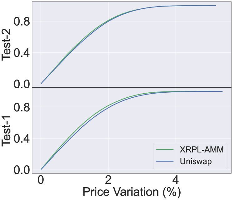
Figure 1: Test-1 and Test-2 cumulative distribution functions of the price sync. with the reference market for xrpl-amm vs. Uniswap.

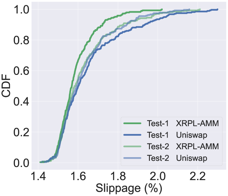
Figure 2: Test-1 and Test-2 cdfs of the slippage.

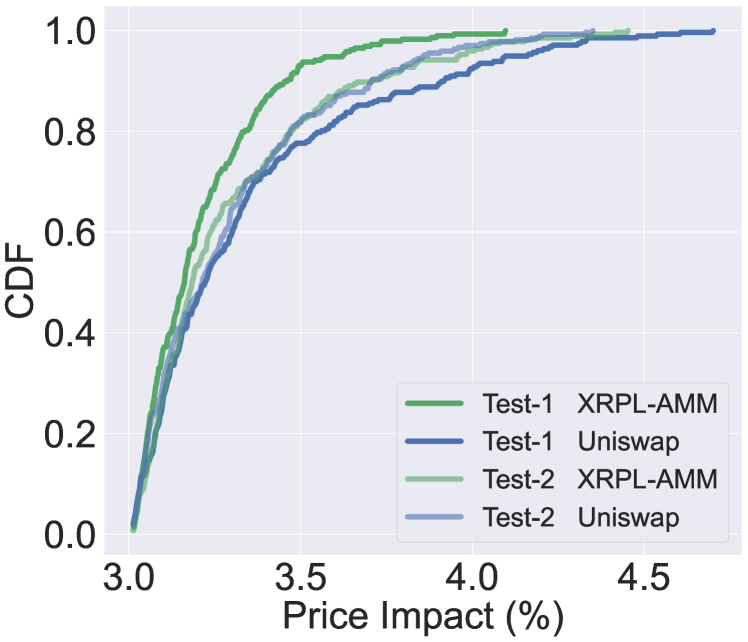
Figure 3: Test-1 and Test-2 CDFs of the price impact.

Arbitrageurs’ Profits, Transaction Cost & Transaction Frequency: Arbitrageurs on xrpl-amm are more profitable in both test scenarios, with a 60% advantage. Specifically, when network fees were equalized, the profits between the two platforms were almost identical, differing by a mere 0.45%, as shown in Table IV. However, when the network fees varied, this profit difference expanded to 4.4%.

TABLE IV: Test-1 and Test-2 average arbitrageurs’ profits, transaction costs & transaction frequency for xrpl-amm vs. Uniswap.

		Profits	Fees	Transaction Count
		(USDC)	(USDC)	Realized	Unrealized
Test-1	xrpl-amm	384,410	29	29 (10%)	260
	Uniswap	382,696	28	28 (4%)	634
Test-2	xrpl-amm	376,272	0.0003	27 (5%)	476
	Uniswap	360,581	107.6	27 (6%)	454

A significant disparity was also evident in transaction fees during Test-2. Arbitrageurs paid 35,866,567% more on Uniswap for the same number of transactions. While the transaction count was relatively consistent across tests, in Test-1, which had varied block times, xrpl-amm registered a single transaction more than Uniswap, representing a 3.6% difference.

Interestingly, even though Uniswap recorded about 2.3 times more placed transactions than xrpl-amm, only 4% of these transactions were realized. In contrast, xrpl-amm showed a 10% realization rate. This gap can be attributed to the maximum slippage condition. The minimized network fees on xrpl contribute to higher arbitrageurs profits than Uniswap. Additionally, xrpl’s faster block interarrival time enables more materialized transactions.

Slippage: The CDFs in Figure 3 illustrate that when block times are equal, arbitrageurs experience nearly identical slippage on both amms. However, the scenario changes when block times differ; arbitrageurs on xrpl-amm encounter less slippage. In Test-1, on Uniswap, 80% of the slippages linger just below 1.8%, whereas they hover around 1.65% on xrpl-amm, marking an 8.8% reduction. This accentuates the advantage of shorter block times on xrpl in diminishing slippage for users.

Trading Volume: The analysis reveals a striking similarity in trading volumes across both amms. This pattern holds particularly true when network fees are equalized and block times vary. Specifically, in Test-1, the trading volume for XRPL-AMM was 170,746,887 USDC, compared to Uniswap’s 170,721,881 USDC, exhibiting a mere 0.015% difference. Meanwhile, Test-2 showed a slightly higher, yet still minimal, 0.23% difference, with XRPL-AMM recording a trading volume of 170,277,799 USDC, and Uniswap at 169,890,854 USDC.

Price Impact: Figure 4 shows how arbitrage transactions impact amm prices. The disparities in Test-1 are more pronounced compared to those in Test-2. When network fees are equalized while block times vary, xrpl-amm demonstrates a less significant price impact than Uniswap. Test-1 reveals a denser concentration of values ranging between 3% and 3.35% for xrpl-amm, with a few outliers extending up to approximately 4.1%. Conversely, Uniswap displays a more uniform distribution, albeit with a cluster of values between 3% and 3.6% and a few outliers reaching up to 4.7%.

The plot for Test-2, characterized by equal block times and disparate transaction fees, exhibits similar distributions of price impact across both amms. The CDF further corroborates this observation in Figure 3, where the curves for both amms in Test-2 nearly overlap, indicating minimal distinction. However, the CDF curves in Test-1 distinctly favor xrpl-amm over Uniswap. While about 80% of the values for xrpl-amm remain below approximately 3.3%, they cap at around 3.55% for Uniswap, translating to a notable 7.6% difference in favor of xrpl-amm. Therefore, it is reasonable to conclude that the diminished price impact on xrpl-amm can be ascribed to its shorter block interarrival time.

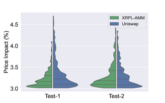
Figure 4: Test-1 and Test-2 price impact (%) caused by arbitrageurs. The dotted lines represent the first, second (mean), and third quartiles.

LPs Returns & Divergence Loss4: In 7 out of the 10 simulation iterations, LPs earned better returns on XRPL-AMM compared to Uniswap, although the difference is minimal, at only around 0.35% more. Specifically, in Test-1, LPs on XRPL-AMM saw average returns of 954,394 USDC with a divergence loss (which in this case translates to a gain) of +1.22%, compared to Uniswap’s returns of 951,561 USDC and a divergence gain of +1.21%. In Test-2, XRPL-AMM LPs experienced returns of 951,984 USDC and a divergence benefit of +1.23%, while Uniswap LPs had returns of 948,364 USDC with a divergence gain of +1.26%. Albeit similar results for divergence loss in both tests indicate a 2.4% higher gain for LPs on Uniswap in Test-2.

Figure 5 illustrates the distribution of these divergence gains for both tests. While the difference is not as apparent in Test-1, Test-2 shows a noticeable skew to the right for most of the values on Uniswap compared to xrpl-amm, indicating slightly higher divergence gains.

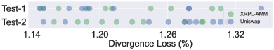
Figure 5: Scatter plot of lps’ divergence gains for Test-1 and Test-2 accross xrpl-amm and Uniswap.

Key Findings: From the results presented above, comparing metrics across the xrpl-amm (without the continuous auction mechanism) and Uniswap, we can derive the following conclusions regarding the behavior of the amms on the two different blockchains:

xrpl’s quicker block interarrival time contributes to better price synchronization with the benchmark market, a higher percentage of realized transactions (transactions placed and successfully executed, passing the slippage condition), reduced slippage, and lower price impact. xrpl’s lower network fees contribute to increased arbitrageurs’ profits and increased trading volume.

It is worth mentioning that when transaction fees and block times are simultaneously equalized, xrpl-amm’s performance nearly mirrors Uniswap’s. In addition, when implementing the cam to these tests, the results are even more in favor of the xrpl amm, regardless of whether fees or block times are equalized.

VII-B2 XRPL-CAM vs Uniswap

We implement the cam with the two distinct strategies previously mentioned in item: xrpl-cam-A (best-case scenario for liquidity providers) and xrpl-cam-B (best-case scenario for arbitrageurs). We conduct three simulations with the same drift $\mu=1\%$ but with a different volatility parameter: $\sigma=10\%$, $\sigma=25\%$, and $\sigma=40\%$.

The objective is to analyze the amms’ performances in the face of increasing volatility, focusing on the profits accrued by arbitrageurs and the returns and divergence loss experienced by LPs. For all other metrics, results between xrpl-cam-A and xrpl-cam-B are substantially identical. The findings are consolidated and represented as xrpl-cam for easy analysis and clarity. Note that while the actual implementation of the xrpl-amm accommodates up to four concurrent users for the auction slot, we reduced this in our tests to only one user for simplicity. Table V shows the parameters used in these simulations.

TABLE V: Simulation parameters for xrpl-cam vs. Uniswap.

Simulation parameters
Parameter	Value
xrpl network fees (USDC)	0.00001
Ethereum network fees (USDC)	4
xrpl block interarrival time	4
Ethereum block interarrival time	12
Safe profit margin (%)	1.5
Maximum slippage (%)	4

Price Synchronization: In our study, the xrpl-cam consistently outperformed Uniswap in maintaining price alignment with the external market at all levels of market volatility, as shown in Figure 8.

Despite the challenge posed by increasing market volatility, xrpl-cam showed superior performance compared to Uniswap at every volatility level tested. Specifically, consider the data points where 80% of the values reside for both amms across the three volatility scenarios: at a volatility of $\sigma=10\%$, the price gap peaked at 1.9% for xrpl-cam and 2.3% for Uniswap. At $\sigma=25\%$, these peaks were 2.5% for xrpl-cam and 3.3% for Uniswap. At the highest tested volatility of $\sigma=40\%$, they were 3.13% and 5%, respectively. The corresponding performance differences between the two amms at these levels were 21%, 32%, and 60%. The faster ledger confirmation time of XRPL, being three times quicker than Ethereum’s allows for more frequent price updates on xrpl.

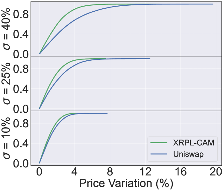
Figure 6: cdfs of the price difference with the external market for three volatilities.

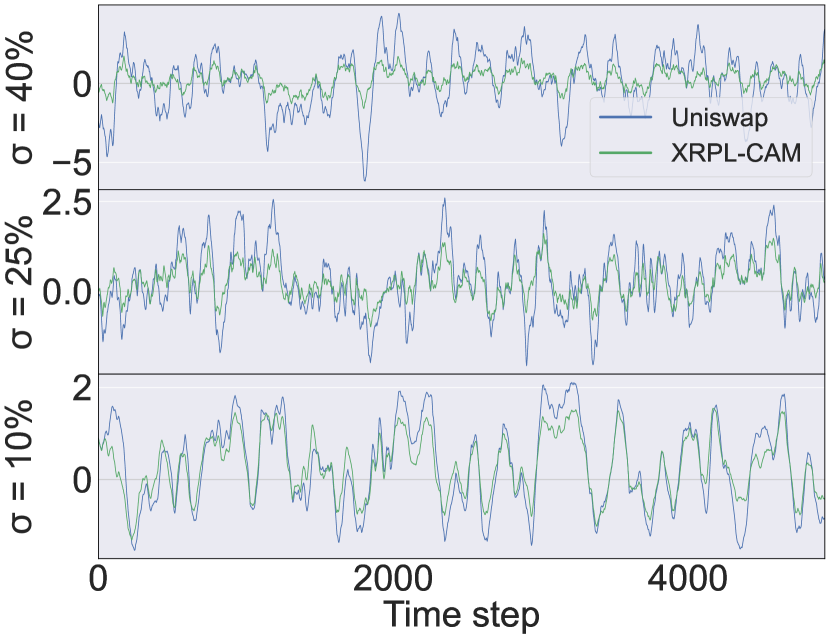
Figure 7: 75-period moving averages of price discrepancies (%) with external markets across three volatilities.

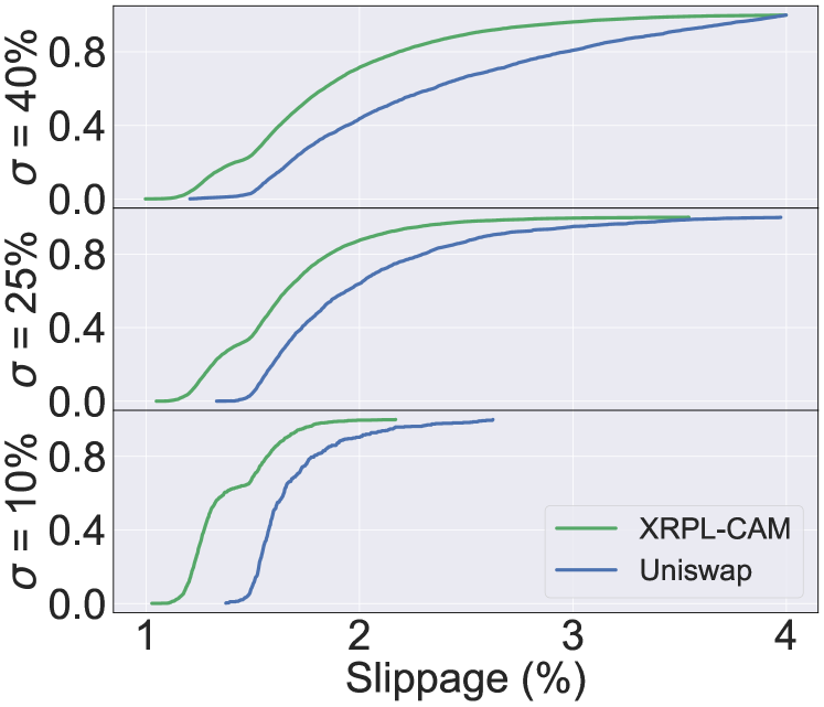
Figure 8: CDFs of the slippage for three volatilities.

Our analysis using a 75-period moving average to track the percentage price divergence from the benchmark market reveals a more stable trend for xrpl-cam compared to Uniswap. As depicted in Figure 8, Uniswap’s moving average shows increased fluctuation with higher volatility, while xrpl-cam’s remains steady, never exceeding a 1.7% divergence across all volatility scenarios.

Arbitrageurs’ Profits, Transaction Cost & Transaction Frequency: In the best-case scenario for arbitrageurs (xrpl-cam-B), they find themselves more profitable 70% of the time when $\sigma=10\%$ and 100% of the time for $\sigma=25\%$ and $\sigma=40\%$ when compared to Uniswap. Conversely, in the worst-case scenario (xrpl-cam-A), they never have an edge over those on Uniswap since most of the profits they could have made went to liquidity providers. Given the data in Table VI below, we can gather the insights in Table VII.

TABLE VI: Average arbitrageurs’ profits, transaction costs & transaction frequency for xrpl-cam vs. Uniswap.

		Profits	Fees	Transaction Count
		(USDC)	(USDC)	Realized	Unrealized
$\sigma=10\%$	xrpl-cam-A	209,421	0.001	59 (19%)	255
	xrpl-cam-B	693,873
	Uniswap	644,759	196	49 (4.5%)	1,028
$\sigma=25\%$	xrpl-cam-A	1,636,246	0.003	268 (12.5%)	1,875
	xrpl-cam-B	5,095,595
	Uniswap	4,507,532	844	211 (4%)	5,131
$\sigma=40\%$	xrpl-cam-A	2,126,299	0.005	516 (11.3%)	4,063
	xrpl-cam-B	13,051,036
	Uniswap	12,560,491	1,680	420 (4%)	9,771

TABLE VII: Insights on Arbitrage Aspects

Insight
Profits: Arbitrageurs earn on average 8% more on XRPL-CAM-B than on Uniswap, but 291% less on XRPL-CAM-A. This disparity lessens as market volatility rises, with increased arbitrage opportunities leading to higher profits.
Transaction Costs: XRPL-CAM features significantly lower transaction fees than Uniswap, leading to notable cost savings. For instance, when $\sigma=25\%$, Uniswap’s network fees were 844 USDC, 28 million percent more than XRPL-CAM’s 0.003 USDC. As market volatility increases, this fee disparity becomes more pronounced, with XRPL-CAM experiencing a slight rise in fees and Uniswap seeing a more noticeable surge.
Transaction Count: XRPL-CAM and Uniswap see increased transaction count (realized and unrealized) with higher volatility. The rate of increase in realized transactions slows as volatility rises. Uniswap typically records unrealized transactions at all volatility levels, suggesting more frequent slippage condition violations. The proportion of realized transactions on XRPL-CAM decreases with growing volatility, whereas Uniswap consistently shows a lower percentage of realized transactions than XRPL-CAM.

Furthermore, we observed that as market volatility escalates, the proportion of transactions executed by auction slot holders diminishes, from 68% for $\sigma=10\%$ to 34% for $\sigma=40\%$. This trend may be attributable to heightened competition and the constraints imposed by the slippage condition, particularly considering that transactions on xrpl are processed in a random order.

Slippage: Due to shorter transaction latency, the xrpl-amm can confirm transaction prices more frequently, resulting in smaller slippages as outlined in Figure 8.

Again, consider the data points where 80% of the values reside for both amms across the three volatility scenarios: for $\sigma=10\%$, the values peak at 1.57% for xrpl-cam and 1.8% for Uniswap; for $\sigma=25\%$, they reach a maximum of 1.86% for xrpl-cam and 2.3% for Uniswap; and for $\sigma=40\%$, they top at approximately 2.18% for xrpl-cam and 2.96% for Uniswap. The difference between the two amms at these volatility levels corresponds to 14.6%, 23.7%, and 35.8%, respectively.

Trading Volume: The trading volume for both XRPL-CAM and Uniswap increases as market volatility escalates, which is expected since higher volatility typically leads to more trading activity as traders seek to capitalize on price differences. It is evident that at every volatility level, XRPL-CAM exhibits higher trading volume compared to Uniswap, averaging 5.6% more, which highlights its superior market efficiency as arbitrageurs trade more and encounter less slippage. Specifically, at a volatility level of 10%, XRPL-CAM’s trading volume is 184,521,310 USDC, compared to Uniswap’s 178,686,957 USDC. At a higher volatility of 25%, XRPL-CAM’s volume increases to 521,687,294 USDC, while Uniswap records 487,266,236 USDC. In the most volatile scenario of 40%, XRPL-CAM sees a trading volume of 1,015,612,864 USDC, significantly higher than Uniswap’s 953,352,684 USDC.

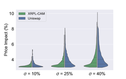
Figure 9: Price impact caused by arbitrageurs under three varying volatilities. The dotted lines represent the first, second (mean), and third quartiles.

Price Impact: Figure 9 demonstrates that price impact increases with market volatility for all amms. Notably, the difference in price impact between xrpl-cam and Uniswap becomes more significant as volatility rises.

At 10% volatility, both amms show similar average price impacts, though Uniswap exhibits more outliers. As volatility increases to 25%, xrpl-cam maintains a lower and more consistent mean price impact than Uniswap. At $\sigma=40\%$, this disparity grows, with Uniswap’s mean price impact being 14% higher than that of xrpl-cam.

Overall, Uniswap experiences a wider spread of price impact values than xrpl-cam. This suggests that trades on Uniswap are likelier to significantly alter prices, whereas xrpl-cam allows for larger trades with less price disturbance. This trend is attributed to the smaller price discrepancies between xrpl-cam and the external market compared to Uniswap, leading to larger necessary arbitrage trades on Uniswap and, consequently, more pronounced price impacts.

LPs Returns & Divergence Loss: As shown in Table VIII, lps gain more returns with increasing market volatility, particularly from cam bids and trading fees. While trading fee returns are lower for xrpl-cam compared to Uniswap due to fee exemptions for auction slot holders, lps on xrpl-cam-A notably outperform those on xrpl-cam-B and Uniswap in high volatility conditions. This is attributed to increased arbitrage bidding, leading to about 170% higher returns for lps on xrpl-cam-A than Uniswap, while those on xrpl-cam-B earn 12% less than Uniswap. The cam enhances lps’ returns under varying market conditions.

TABLE VIII: Average LPs’ returns under different volatilities.

		cam bids returns	Trading fees returns	Total
		(USDC)	(USDC)	(USDC)
$\sigma=10\%$	xrpl-cam-A	533,306 (38%)	869,945 (62%)	1,403,251
	xrpl-cam-B	12,170	871,324	883,494
	Uniswap	NA	945,589	945,589
$\sigma=25\%$	xrpl-cam-A	4,111,154 (69%)	1,861,343 (31%)	5,972,497
	xrpl-cam-B	17,593	1,856,295	1,873,888
	Uniswap	NA	2,120,726	2,120,726
$\sigma=40\%$	xrpl-cam-A	10,979,267 (78%)	3,169,108 (22%)	14,148,375
	xrpl-cam-B	16,395	3,184,098	3,200,493
	Uniswap	NA	3,710,291	3,710,291

In xrpl-cam-A, returns from the cam increasingly contribute to total returns with higher market volatility, reaching 78% at $\sigma=40\%$. This indicates that arbitrageurs bid aggressively in volatile markets, taking advantage of price fluctuations.

At all volatility levels, lps in xrpl-cam-A consistently show less divergence loss or more gain than xrpl-cam-B and Uniswap. For example, at $\sigma=10\%$, xrpl-cam-A lps experience a +2.26% divergence gain, outperforming Uniswap’s +1.87% and xrpl-cam-B’s +1.74%. This difference becomes more marked with increasing volatility. At $\sigma=25\%$, xrpl-cam-A’s divergence loss is -1.13%, much lower than xrpl-cam-B’s -3.96% and Uniswap’s -3.24%. At $\sigma=40\%$, the divergence gain for xrpl-cam-A soars to +8%, significantly exceeding Uniswap’s -0.38% loss and xrpl-cam-B’s +0.2%.

Figure 10 visually illustrates this trend, showing that divergence loss/gain disparities between xrpl-cam-A and the others grow with increasing volatility. xrpl-cam-B’s performance in divergence loss/gain closely mirrors that of Uniswap across various volatility levels, indicating comparable worst-case scenarios for lps in both amms.

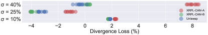
Figure 10: Divergence loss/gain for xrpl-cam vs. Uniswap with different volatilities.

Key Findings: From the results discussed above, comparing metrics across xrpl-cam (xrpl-amm with cam) and Uniswap, we can derive the following conclusions regarding the behavior of the amms on the two different blockchains: xrpl-cam contributes to (a) better price synchronization with the external market, (b) a higher percentage of materialized transactions (transactions placed and successfully executed, passing the slippage condition), (c) reduced slippage, (d) lower price impact, (e) increased trading volume and (f) lower transaction fees.

Our analysis shows different outcomes for lps and arbitrageurs in both best-case and worst-case scenarios. For lps, the best-case scenario on xrpl-cam yields higher returns and lower divergence loss compared to Uniswap, while the worst-case scenario shows the opposite. For arbitrageurs, the best case on xrpl-cam brings more profits than Uniswap, but in the worst case, they fare better on Uniswap. However, in realistic market conditions with balanced arbitrage strategies, arbitrageurs might see fewer profits on xrpl-cam, while lps could benefit from higher earnings and reduced divergence loss, particularly in volatile markets. This analysis combines the best and worst-case scenarios to reflect typical market behaviors.

VIII Conclusion

This study tested the xrpl-amm, which addresses challenges in existing Ethereum-based amms. The results of this paper validate the xrpl-amm’s potential to reshape the defi sector. The xrpl-amm, capitalizing on xrpl’s efficiency, outperforms Ethereum counterparts like Uniswap in areas including slippage and divergence loss reduction. Its unique cam promotes swift price synchronization with external markets by rewarding beneficial arbitrage. While volatility typically holds negative connotations, the xrpl-amm leverages it, allowing arbitrageurs to harvest it for mutual benefit. Therefore, our research not only enriches the defi ecosystem but also accentuates xrpl-amm’s promise for defi.

References

- [1] D. Zetzsche, D. Arner, and R. Buckley, “Decentralized finance,” 2020. [Online]. Available: https://academic.oup.com/jfr/article/6/2/172/5913239
- [2] S. Kitzler, F. Victor, P. Saggese, and B. Haslhofer, “Disentangling decentralized finance (defi) compositions,” 2023. [Online]. Available: https://dl.acm.org/doi/10.1145/3532857
- [3] K. Shah, D. Lathiya, N. Lukhi, K. Parmar, and H. Sanghvi, “A systematic review of decentralized finance protocols,” 2023. [Online]. Available: https://www.sciencedirect.com/science/article/pii/S2666603023000179
- [4] D. Metelski and J. Sobieraj, “Decentralized finance (defi) projects: A study of key performance indicators in terms of defi protocols’ valuations,” 2022. [Online]. Available: https://www.mdpi.com/2227-7072/10/4/108
- [5] H. Eyal, G. Benartzi, and G. Benartzi, “Bancor whitepaper,” 2017. [Online]. Available: https://www.allcryptowhitepapers.com/bancor-whitepaper/
- [6] H. Adams, N. Zinsmeister, M. Salem, R. Keefer, and D. Robinson, “Uniswap whitepaper,” 2023. [Online]. Available: https://uniswap.org/whitepaper-v3.pdf
- [7] A. Othman, “Automated market making: Theory and practice,” 2012. [Online]. Available: http://reports-archive.adm.cs.cmu.edu/anon/2012/CMU-CS-12-123.pdf
- [8] L. Heimbach, E. Schertenleib, and R. Wattenhofer, “Exploring price accuracy on uniswap v3 in times of distress,” 2022. [Online]. Available: https://arxiv.org/pdf/2208.09642.pdf
- [9] B. Ghosh, H. Kazouz, and Z. Umar, “Do automated market makers in defi ecosystem exhibit time-varying connectedness during stressed events?” 2023. [Online]. Available: https://www.mdpi.com/1911-8074/16/5/259
- [10] J. Xu, K. Paruch, S. Cousaert, and Y. Feng, “Sok: Decentralized exchanges (DEX) with automated market maker (AMM) protocols,” ACM Comput. Surv., vol. 55, no. 11, 2 2023. [Online]. Available: https://doi.org/10.1145/3570639
- [11] A. Malhotra and D. J. Schwartz, “0030 xls 30d: Automated market maker on xrpl,” 2022. [Online]. Available: https://github.com/XRPLF/XRPL-Standards/discussions/78
- [12] S. P. Lee, “Market share of decentralized crypto exchanges, by trading volume — coingecko,” 2023. [Online]. Available: https://www.coingecko.com/research/publications/decentralized-crypto-exchanges-market-share
- [13] G. Angeris, H.-T. Kao, R. Chiang, C. Noyes, and T. Chitra, “An analysis of uniswap markets,” 2019. [Online]. Available: https://arxiv.org/pdf/1911.03380.pdf
- [14] J. Xu and Y. Feng, “Reap the harvest on blockchain: A survey of yield farming protocols,” IEEE Transactions on Network and Service Management, vol. 20, no. 1, pp. 858–869, 2023.
- [15] H. Adams, N. Zinsmeister, and D. Robinson, “Uniswap v2 core,” 2020.
- [16] Ripple, “Xrpl oldest dex,” 2023. [Online]. Available: https://xrpl.org/decentralized-exchange.html
- [17] I. Gemeliarana and R. Sari, “Evaluation of proof of work (pow) blockchains security network on selfish mining,” 2019. [Online]. Available: https://ieeexplore.ieee.org/document/8864381
- [18] A. Sirio, W. Huang, and A. Schrimpf, “Trading in the defi era: automated market-maker,” 2021. [Online]. Available: https://www.bis.org/publ/qtrpdf/r_qt2112v.htm
- [19] V. Tumas, B. Fiz Pontiveros, C. Torres, and R. State, “A ripple for change: Analysis of frontrunning in the xrp ledger,” 05 2023.
- [20] Ripple, “Xrpl overview,” 2023. [Online]. Available: https://xrpl.org/xrp-ledger-overview.html
- [21] Ethereum.org, “Ethereum blocks,” 2023. [Online]. Available: https://ethereum.org/en/developers/docs/blocks/
- [22] Ripple, “Xrpl transaction cost,” 2023. [Online]. Available: https://xrpl.org/transaction-cost.html
- [23] G. Peduzzi, J. James, and J. Xu, “Jack the rippler: Arbitrage on the decentralized exchange of the xrp ledger,” 2021. [Online]. Available: https://ieeexplore.ieee.org/document/9569833
- [24] Ripple Open Source, “Automated market maker,” 2023. [Online]. Available: https://opensource.ripple.com/docs/xls-30d-amm/amm-uc/
- [25] “Uniswap v3 (ethereum) trade volume, trade pairs & trust score — coingecko.” [Online]. Available: https://www.coingecko.com/en/exchanges/uniswap-v3-ethereum
- [26] “Uniswap pools.” [Online]. Available: https://info.uniswap.org/#/pools
- [27] R. Marathe and S. Ryan, “On the validity of the geometric brownian motion assumption,” 2007. [Online]. Available: https://www.tandfonline.com/doi/full/10.1080/00137910590949904
- [28] J. Song, Z. Duan, and W. Lyu, “Research on geometric brownian motion and its practice in pricing,” 2022. [Online]. Available: https://dl.acm.org/doi/pdf/10.1145/3523181.3523204
- [29] J. Lidén, “Stock price predictions using a geometric brownian motion,” 2018. [Online]. Available: https://www.diva-portal.org/smash/get/diva2:1218088/FULLTEXT01.pdf
- [30] V. Moroz and I. Yalymova, “Modeling the volatity of cryptocurrency markets,” 2021. [Online]. Available: https://repository.kpi.kharkov.ua/server/api/core/bitstreams/2fcc0db4-f97d-4079-b090-c4e1e415de8f/content
- [31] E. Bouri, R. Gupta, and D. Roubaud, “Herding behaviour in cryptocurrencies,” Finance Research Letters, vol. 29, pp. 216–221, 6 2019.
- [32] T. King and D. Koutmos, “Herding and feedback trading in cryptocurrency markets,” Annals of Operations Research, vol. 300, pp. 79–96, 5 2021. [Online]. Available: https://link.springer.com/article/10.1007/s10479-020-03874-4
- [33] Y. Liu and A. Tsyvinski, “Risks and returns of cryptocurrency,” 2018. [Online]. Available: https://www.nber.org/system/files/working_papers/w24877/w24877.pdf
- [34] Etherscan, “Gas tracker,” 2023. [Online]. Available: https://etherscan.io/gastracker#historicaldata
- [35] Poolfish, “Ethereum fees,” 2023. [Online]. Available: https://poolfish.xyz/