Millimeter-wave Radio SLAM: End-to-End Processing Methods and Experimental Validation

Abstract

In this article, we address the timely topic of cellular bistatic simultaneous localization and mapping (SLAM) with specific focus on complete processing solutions from raw I/Q samples to user equipment (UE) and landmark location information in millimeter-wave (mmWave) networks. Firstly, we propose a new multipath channel parameter estimation solution which operates directly with beam reference signal received power (BRSRP) measurements, alleviating the need to know the true antenna beampatterns or the underlying beamforming weights. Additionally, the method has built-in robustness against unavoidable antenna sidelobes. Secondly, we propose new snapshot SLAM algorithms that have increased robustness and identifiability compared to prior-art, in practical built environments with complex clutter and multi-bounce propagation scenarios. The performance of the proposed methods is assessed at the 60 GHz mmWave band, via both realistic ray-tracing evaluations as well as true experimental measurements, in an indoor environment. Wide set of offered results clearly demonstrate the improved performance, compared to the relevant prior-art, in terms of the channel parameter estimation as well as the end-to-end SLAM performance. Finally, the article provides the measured 60 GHz data openly available for the research community, facilitating results reproducibility as well as further algorithm development.

I Introduction

W hile the primary purpose of mobile cellular networks is to provide efficient connectivity services, the ability to extract location information and situational awareness of the surrounding environment is also receiving increasing interest [1, 2, 3, 4]. The related notion of integrated sensing and communications (ISAC) refers to extending the situational awareness from ordinary user equipment (UE) positioning to the ability to sense also various passive objects in the environment, through cellular radio-based measurements and corresponding signal processing [5, 1]. Such knowledge of the UE locations and surrounding environment can be harnessed in numerous ways, for example in different extended reality (XR) use cases [6], vehicular applications [7], or industrial systems [8]. In general, the prospects for high-accuracy situational awareness are known to improve [9, 10] when the networks are expanding towards the millimeter-wave (mmWave) frequency bands. The current fifth generation New Radio (5G NR) specifications support already operating bands up to 71 GHz [11], while further extensions towards the sub-THz regime are expected in the 6G era [12].

Bistatic cellular simultaneous localization and mapping (SLAM) is one of the most prominent, yet technically challenging ISAC scenarios where the coordinates of both the UE as well as those of the environment scattering points – commonly referred to as the landmarks – are all jointly estimated, based on either uplink (UL) or downlink (DL) reference signals and known base-station (BS) locations [13, 14, 15]. This is illustrated conceptually in Fig. 1. Complete end-to-end solutions for SLAM comprise estimators for spatio-temporal channel parameters, often in the form of time of arrival (ToA), angle-of-arrival (AoA), and/or angle-of-departure (AoD) of the involved propagation paths, combined with the actual SLAM filters or snapshot estimators that process the channel parameter estimates into the corresponding estimates of the UE and landmark locations [16]. This is also the main scope of this article. We have specific focus on implementation-feasible yet high-performing end-to-end processing solutions that can operate with minimal knowledge of the involved antenna system beampatterns and facilitate mmWave SLAM in practical complex built environments, particularly indoors, while operating on downlink positioning reference signal (PRS) standardized already for the existing 5G NR networks. Additionally, we emphasize research reproducibility and provide measured mmWave I/Q and channel data openly for the research community, while use the same measured data to evaluate and benchmark the proposed methods against the relevant prior art.

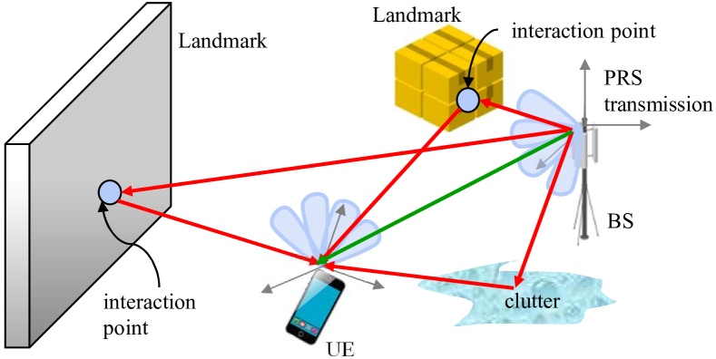
Figure 1: Illustration of the bistatic cellular SLAM paradigm where UE is jointly estimating its own state as well as those of the environment landmarks.

I-A Prior Art

The available literature on channel parameter estimation is generally-speaking wide, however, a vast majority of works is carried out under the assumptions of known antenna steering vectors, beamforming weights, and thereon beampatterns. Such methods are described, e.g., in [17, 18, 19, 20, 21, 22, 23, 24, 25]. To this end, [17] and [18] present Bayesian channel estimation algorithms based on different variants of Kalman filters, while [19, 21, 22] harness the mmWave channel sparsity through compressed sensing (CS) methods. The work in [20], in turn, proposes an AoA estimation method using virtual subarrays which, however, requires a special beamformer or antenna pattern design, similar to [23]. Furthermore, [24, 25] propose joint AoD and AoA estimation methods with specific frequency-dependent codebooks in true-time-delay array context. Opposed to these previous works, an angle estimation algorithm building on the beam reference signal received power (BRSRP) measurements is described in the recent work in [15]. The method builds on thresholding and successive cancellation principle, operating on AoA-AoD power map, however, is lacking, e.g., explicit treatment of antenna sidelobes whose impact can be substantial in mmWave systems. This is particularly so in SLAM context where the multipaths and their dynamic range is one key factor. For clarity, we also note that works like [26] exist that deploy machine-learning to the channel parameters estimation – however, such works are still commonly at their early phases.

In the context of the available SLAM methods, we first note that both snapshot approaches [16, 27, 28, 29] as well as sequential filtering based solutions [30, 13, 14, 15, 31] exist. Both research directions are relevant and the preferred choice depends on the overall system and application scenario. Snapshot SLAM is fundamentally important as it serves as a baseline for what can be done with radio signals alone, without any movement models, while a snapshot method can also be used as input to filtering [27]. On the other hand, filtering based SLAM methods process the observations sequentially over time and are expected to remove false detections and improve the accuracy [14]. Both SLAM methods also have their limitations. A major drawback of snapshot SLAM is that it is not always applicable, since the measurements may not be sufficient to solve the SLAM problem [16]. For example, the UE cannot be localized with the line-of-sight (LoS) alone if the clocks of the UE and BS are not synchronized [27] and one must resort to filtering based techniques to solve the problem over time. On the other hand, filtering methods always require a snapshot algorithm for initialization when prior information is not available. Another disadvantage of filtering methods is that they require solving a complex data association problem which increases computational overhead of the algorithms [14, 31]. It is to be noted that low complexity alternatives exist [30, 13], however, at the expense of reduced accuracy.

I-B Novelty and Contributions

Compared to the available methods and literature, this article provides the following contributions. Firstly, opposed to the vast majority of existing literature in [17, 18, 19, 20, 21, 22, 23, 24, 25], we focus on enabling accurate multipath AoA/AoD estimation with BRSRP measurements only, without knowledge of the complex antenna patterns or the underlying steering vectors and beamforming weights. This is motivated by the fact that in real networks, only the beam indices and corresponding nominal beam directions are commonly available [32]. Furthermore, various practical aspects such as errors in the antenna element spacings as well as mutual coupling create anyway varying levels of uncertainties in the true antenna patterns – in particular in mmWave networks [33] where analog/RF beamforming dominates and the design and implementation of antenna elements and beamforming units is tedious. Additionally, the proposed channel parameter estimator that builds on the singular value decomposition (SVD) of the AoA-AoD BRSRP map is shown to have built-in robustness against the antenna sidelobes which is a clear additional benefit compared to the prior art in [15]. The proposed method is also compatible with 5G NR PRS signal structure and beam-sweaping procedures [34].

Secondly, we focus on advancing the robustness and tolerance of snapshot SLAM, compared to the prior art in [16, 28, 29], against practical measurement imperfections or outliers while also seek to improve the SLAM problem identifiability. These aspects have high importance in real mmWave deployment environments, where the amount of the available LoS/non-line-of-sight (NLoS) measurements can easily vary from measurement location to another [35]. Additionally, despite the advances in channel parameter estimation, measurement outliers are commonly occurring, e.g., due to the clutter, multi-bounce phenomenon and antenna sidelobes [5]. Specifically, we improve the snapshot SLAM identifiability via including an appropriate regularization term into the objective function that embeddes the prior information to the processing system. Additionally, a robust cost function is introduced to handle outliers originating, e.g., from false detections or clutter.

Finally, the openly available mmWave SLAM measurement data is scarce – or almost non-existing – hence, we bridge this important gap and provide 60 GHz indoor measurement data building on 5G NR standard-compliant beam-based PRS transmissions. We also utilize the measurement data to assess the achievable end-to-end performance of the methods proposed in this article, while benchmarking against the prior-art.

Thus, to summarize, the novelty and contributions of the article can be shortly stated as follows:

• We propose a new propagation path AoA/AoD estimation method utilizing standardized BRSRP measurements, alleviating the need for knowledge of the underlying antenna system beampatterns while offering controlled robustness against antenna sidelobes;

• We propose a new snapshot SLAM algorithm that offers increased system identifiability and improved robustness against measurement outliers compared to prior-art;

• We evaluate and benchmark the performance of the proposed methods in a realistic indoor environment through accurate ray-tracing as well as experimental measurement campaign, both carried out at the 60 GHz band;

• We release the complete 60 GHz I/Q measurement data set as well as the corresponding processed channel parameter data set, together with supportive scripts for their utilization in any follow-up research;

The rest of this article is organized as follows: Section II describes the basic assumptions, the problem geometry and the corresponding fundamental system model. The proposed channel parameter estimation methods are described in Section III, while the proposed snapshot SLAM method is provided in Section IV. The considered indoor evaluation environment, ray-tracing assumptions and the actual 60 GHz measurement setup and data are all described in Section V. The complete end-to-end performance results and corresponding comparisons against benchmark methods are reported and analyzed in Section VI. Finally, the conclusions are drawn in VII, while selected modeling details are provided in the Appendix.

Notations: Vectors are denoted by bold lowercase letters (i.e., $\mathbf{a}$), bold uppercase letters are used for matrices (i.e., $\mathbf{A}$) and scalars are denoted by normal font (i.e., $a$). The operators $(\cdot)^{\top}$, $(\cdot)^{*}$, $(\cdot)^{\mathrm{H}}$, $(\cdot)^{\dagger}$, $\mathbb{E}\{\cdot\}$, $|\cdot|$ and $\|\cdot\|$ denote the transpose, conjugate, Hermitian transpose, pseudoinverse, expectation, absolute value and Euclidian norm, respectively. Finally, $\mathrm{i}$ denotes the imaginary unit for which $\mathrm{i}^{2}=-1$.

II System Model

II-A Basic Assumptions and System Geometry

In this work, we consider orthogonal frequency-division multiplexing (OFDM) based mmWave cellular systems where BSs are regularly broadcasting beamformed downlink reference signals, that allow UEs to estimate the multipath channel parameters for localization, sensing and mapping purposes. Concrete example in 5G NR context is the PRS [34], however, also e.g. the synchronization signal (SS) burst can in practice be utilized, though offering lower bandwidth compared to PRS. Additionally, since time- and angle-based measurements allow for a paradigm shift from classical multi-BS localization and SLAM approaches [7] towards single-BS solutions [36], we also focus on the single-BS scenario. However, the proposed channel parameter estimator is applicable also in multi-BS scenarios when the corresponding PRSs are properly orthogonalized.

To this end, we consider transmitter (TX) and receiver (RX) entities equipped with uniform planar arrays (UPAs) with vertical times horizontal dimensions of the form ${N}^{v}_{\textrm{TX}}\times{N}^{h}_{\textrm{TX}}$ and ${N}^{v}_{\textrm{RX}}\times{N}_{\textrm{RX}}^{h}$, respectively. The antenna elements are separated by a half-wavelength distance $d=\lambda/2$, where $\lambda=\text{c}/f_{c}$ denotes the wavelength at carrier frequency $f_{c}$, and c is the speed of light. The total number of antenna elements in TX and RX are ${N}_{\textrm{TX}}={N}^{v}_{\textrm{TX}}\times{N}^{h}_{\textrm{TX}}$ and ${N}_{\textrm{RX}}={N}^{v}_{\textrm{RX}}\times{N}_{\textrm{RX}}^{h}$, respectively. The locations (3D coordinates) of the involved TX and RX entities are denoted by ${\mathbf{p}}_{\textrm{TX}}^{\textrm{3D}}=[{\mathbf{p}}_{\textrm{TX}}^{\top},\,z_{\textrm{TX}}]^{\top}$ and ${\mathbf{p}}_{\textrm{RX}}^{\textrm{3D}}=[{\mathbf{p}}_{\textrm{RX}}^{\top},\,z_{\textrm{RX}}]^{\top}$, respectively, where ${\mathbf{p}}_{\textrm{TX}}$ and ${\mathbf{p}}_{\textrm{RX}}$ are the corresponding 2D coordinates, all in global coordinate system. Additionally, the 3D location of an arbitrary single-bounce landmark is denoted by ${\mathbf{m}}_{n}^{\textrm{3D}}=[{\mathbf{m}}_{n}^{\top},\,z_{n}]^{\top}$ where ${\mathbf{m}}_{n}$ refers to the respective 2D coordinates while the subscript $n$ serves as a landmark or path index. Furthermore, we denote the 3D AoD as $\boldsymbol{\psi}^{\top}_{\text{TX},n}=[\theta_{n},\theta_{n}^{\text{EL}}]$, where $\theta_{n}$ and $\theta_{n}^{\text{EL}}$ are the azimuth and elevation AoDs, respectively, Similarly, the 3D AoA is denoted by $\boldsymbol{\psi}^{\top}_{\text{RX},n}=[\phi_{n},\phi_{n}^{\text{EL}}]$. All the involved angles are expressed in local coordinate systems, i.e., relative to the local orientations of the TX and RX entities.

Finally, as our main emphasis is on indoor mmWave systems, we eventually focus mostly on 2D (azimuth) estimation and SLAM algorithms. The corresponding 2D system geometry is illustrated in Fig. 2. However, the basic system and received signal models are provided in 3D for generality.

II-B Received Signal Model

We assume that coarse timing information is established between TX and RX entities, through, e.g., correlation with known PRS sequences as discussed further in Section III. Now, under multipath radio propagation environment with $N$ propagation paths, the received signal at $k^{\text{th}}$ subcarrier and $m^{\text{th}}$ OFDM symbol, using the $i^{\text{th}}$ TX beam and $j^{\text{th}}$ RX beam, can be represented as

$$y_{k,m}^{i,j}=\mathbf{w}_{\text{RX},j}^{\mathrm{H}}\left(\mathbf{H}_{k,m}\mathbf{w}^{*}_{\text{TX},i}x_{k,m}^{i,j}+\mathbf{n}_{k,m}^{i,j}\right),$$ (1)

where $\mathbf{w}_{\text{TX},i}\in\mathbb{C}^{\text{N}_{\textrm{TX}}}$ and $\mathbf{w}_{\text{RX},j}\in\mathbb{C}^{\text{N}_{\textrm{RX}}}$ are the TX and RX beamformers, $x_{k,m}\in\mathbb{C}$ with $|x_{k,m}|=1\,\forall k,m$ is the transmitted PRS sample, and $\mathbf{n}_{k,m}^{i,j}\in\mathbb{C}^{\text{N}_{RX}}$ denotes the antenna element wise additive white Gaussian noise (AWGN) at the RX. Furthermore, $\mathbf{H}_{k,m}\in\mathbb{C}^{\text{N}_{\textrm{RX}}\times\text{N}_{\textrm{TX}}}$ is the spatial multipath channel matrix defined as [35, eq. (4)]

$$\begin{split}\mathbf{H}_{k,m}=\sum_{n=1}^{N}&\xi_{n}e^{-\mathrm{i}2\pi k\Delta f\tau_{n}}e^{\mathrm{i}2\pi mT_{\text{sym}}f_{\text{D},n}}\\ &\times\mathbf{a}_{\text{RX}}(\boldsymbol{\psi}_{\text{RX},n})\mathbf{a}_{\text{TX}}(\boldsymbol{\psi}_{\text{TX},n})^{\top},\end{split}$$ (2)

where $\Delta f$ is the subcarrier spacing (SCS), $T_{\text{sym}}$ denotes the OFDM symbol duration, and $\xi_{n}$, $\tau_{n}$ and $f_{\text{D},n}$ are the complex path coefficient, the propagation delay, and the Doppler frequency for the $n^{\text{th}}$ propagation path, respectively. The delay $\tau_{n}$ maps to the corresponding propagation distance as $d_{n}=c\tau_{n}$. Additionally, $\mathbf{a}_{\text{TX}}(\boldsymbol{\psi}_{\text{TX},n})\!\in\!\mathbb{C}^{N_{\text{TX}}}$ and $\mathbf{a}_{\text{RX}}(\boldsymbol{\psi}_{\text{RX},n})\!\in\!\mathbb{C}^{N_{\text{RX}}}$ denote the TX and RX steering vectors, respectively. The exact way how the PRS sequences are mapped to the physical resources (OFDM symbols and the underlying subcarriers), in 5G NR context, is described in [34].

Figure 2: Problem geometry for LoS and $n$th NLoS propagation path with angles expressed in the local frames of the TX (BS) and RX (UE). $\alpha_{\textrm{TX}}$ and $\alpha_{\textrm{RX}}$ represent the location orientations relative to the global coordinate system.

Now, by combining (1) and (2), the received signal model can be re-expressed as

$$\begin{split}y_{k,m}^{i,j}=\Big{\{}\sum_{n=1}^{N}&\xi_{n}e^{-\mathrm{i}2\pi k\Delta f\tau_{n}}e^{\mathrm{i}2\pi mT_{\text{sym}}f_{\text{D},n}}x_{k,m}^{i,j}\\ &\times G_{\text{TX},i}(\boldsymbol{\psi}_{\text{TX},n})G_{\text{RX},j}(\boldsymbol{\psi}_{\text{RX},n})\Big{\}}+\tilde{n}_{k,m}^{i,j},\end{split}$$ (3)

where $\tilde{n}_{k,m}^{i,j}=\mathbf{w}_{\text{RX},j}^{\mathrm{H}}\mathbf{n}_{k,m}^{i,j}$ denotes beamformed noise, while $G_{\text{TX},i}(\boldsymbol{\psi}_{\text{TX},n})=\mathbf{a}_{\text{TX}}(\boldsymbol{\psi}_{\text{TX},n})\!{{}^{\top}}\!\mathbf{w}^{*}_{\text{TX},i}$, and $G_{\text{RX},j}(\boldsymbol{\psi}_{\text{RX},n})=\mathbf{w}_{\text{RX},j}^{\mathrm{H}}\mathbf{a}_{\text{RX}}(\boldsymbol{\psi}_{\text{RX},n})$. Importantly, the expression in (3) applies to arbitrary antenna systems with $G_{\text{TX},i}(\boldsymbol{\psi}_{\text{TX},n})\!\in\!\mathbb{C}$ and $G_{\text{RX},j}(\boldsymbol{\psi}_{\text{RX},n})\!\in\!\mathbb{C}$ denoting the corresponding angular responses for the $i^{\text{th}}$ and $j^{\text{th}}$ beams at the TX and RX sides.

The fundamental technical problems considered in the article are (i) to estimate the involved path angles and delays, with received PRS samples, and (ii) to estimate the UE location and the locations of the landmarks, with angle and delay estimates as the inputs. These are addressed in Sections III and IV, respectively, where Section IV also details the relations between the locations and the involved path angles and delays.

III Channel Parameter Estimation Methods

In this section, we provide a detailed description of the proposed AoA/AoD estimation method, along with an explanation of the ToA estimation approach we have considered. To ensure clarity and simplify the presentation, we focus on describing these methods in the 2D/azimuth domain. This approach is particularly relevant in indoor scenarios, where the floor and ceiling impose constraints on the extent of the vertical direction. We further assume that directional mmWave beams are deployed, such that the TX and RX beam indices $i$ and $j$ have physical correspondence to the TX and RX beamforming angles, respectively. Such directional beams are considered in large majority of the mmWave systems research, particularly when analog/RF beamforming is assumed.

III-A BRSRP Measurements

Taking reference signal received power (RSRP) measurements is generally a standard procedure in 5G NR [37], e.g., for paging and beam alignment purposes. To this end, for each TX-RX beam pair $(i,j)$, let us define the corresponding BRSRP as a beam-based RSRP measurement of the considered reference signal (RS). Specifically, this is defined as

$$\beta_{i,j}=\frac{1}{{N}_{\text{RS}}}\sum_{(k,m)\in\mathcal{M}_{\text{RS}}}\left|y_{k,m}^{i,j}\right|^{2},$$ (4)

where $\mathcal{M}_{\text{RS}}$ is a set of all RS symbols and subcarriers mapped to the OFDM resource grid with cardinality $|\mathcal{M}_{\text{RS}}|=N_{\text{RS}}$.

Lemma 1.

Let $\mathbf{b}_{n}\in\mathbb{C}^{K}$ and $\mathbf{c}_{n}\in\mathbb{C}^{M}$ denote the frequency-domain and time-domain steering vectors of the $n^{\text{th}}$ path, respectively, where $K$ is the number of active RS subcarriers, and $M$ is the number of RS OFDM symbols. Moreover, the $k^{\text{th}}$ element of $\mathbf{b}_{n}$ is defined as $\mathbf{b}_{n}[k]=e^{-\mathrm{i}2\pi k\Delta f\tau_{n}}$, and the $m^{\text{th}}$ element of $\mathbf{c}_{n}$ as $\mathbf{c}_{n}[m]=e^{\mathrm{i}2\pi mT_{\text{sym}}f_{\text{D},n}}$. Suppose that the paths in (2) are non-overlapping in either delay or Doppler, and that $K$ and/or $M$ are/is sufficiently large, i.e.,

$$\mathbf{b}_{n_{1}}^{\mathrm{H}}\mathbf{b}_{n_{2}}\approx 0~{}~{}~{}{\rm{or}}~{}~{}~{}\mathbf{c}_{n_{1}}^{\mathrm{H}}\mathbf{c}_{n_{2}}\approx 0$$ (5)

for any $n_{1}\neq n_{2}$. Then, the BRSRP measurement in (4) can be approximated as

$$\beta_{i,j}\approx\!\sum_{n=1}^{N}|\xi_{n}|^{2}|G_{\mathrm{TX},i}(\boldsymbol{\psi}_{\mathrm{TX},n})|^{2}|G_{\mathrm{RX},j}(\boldsymbol{\psi}_{\mathrm{RX},n})|^{2}\!+\!\bar{N}_{i,j}$$ (6)

where $\bar{N}_{i,j}=(1/N_{\mathrm{RS}})\sum_{(k,m)\in\mathcal{M}_{\mathrm{RS}}}|\tilde{n}_{k,m}^{i,j}|^{2}$ denotes the averaged noise power.

Proof.

Please see the Appendix. ∎

III-B Proposed SVD-based AoD and AoA Extraction

Considering the PRS beam-sweeping procedure with $L_{\textrm{TX}}$ TX beams and $L_{\textrm{RX}}$ RX beams, comprising the corresponding TX and RX beamforming angles $\{\Phi_{i}\}_{i=1}^{L_{\text{TX}}}$ and $\{\Theta_{j}\}_{j=1}^{L_{\text{RX}}}$, respectively, a total of $L_{\textrm{TX}}\times L_{\textrm{RX}}$ directional BRSRP measurements are available at the RX. The corresponding BRSRP matrix $\mathbf{B}\in\mathbb{R}^{L_{\textrm{TX}}\times L_{\textrm{RX}}}$ is defined as

$$\mathbf{B}=\begin{pmatrix}\beta_{1,1}&\beta_{1,2}&\cdots&\beta_{1,L_{\textrm{RX}}}\\ \beta_{2,1}&\beta_{2,2}&\cdots&\beta_{2,L_{\textrm{RX}}}\\ \vdots&\vdots&\ddots&\vdots\\ \beta_{L_{\textrm{TX}},1}&\beta_{L_{\textrm{TX}},2}&\cdots&\beta_{L_{\textrm{TX}},L_{\textrm{RX}}}\\ \end{pmatrix}.$$ (7)

The matrix $\mathbf{B}$ thus represents the spatial channel in the angular domain, in the form of an AoD-AoA power map. A concrete example is visualized in Fig. 3, building on measurement arrangements described in Section V.

III-B1 Technical Premise and Intuition

Taking into account the fairly narrow beamwidths and the mmWave channel sparsity, the AoDs $\{\phi_{n}\}_{n=1}^{N}$ and AoAs $\{\theta_{n}\}_{n=1}^{N}$ for $N$ propagation paths can be extracted by processing the power map $\mathbf{B}$. For this purpose, based on (4) and the approximation in (6), the angular power map $\mathbf{B}$ can be first represented as

$$\mathbf{B}=\sum_{n=1}^{N}|\xi_{n}|^{2}\mathbf{g}_{\text{TX}}(\boldsymbol{\psi}_{\text{TX},n})\mathbf{g}_{\text{RX}}(\boldsymbol{\psi}_{\text{RX},n})^{\top}+\bar{\mathbf{N}},$$ (8)

where $\mathbf{g}_{\text{TX}}(\boldsymbol{\psi}_{\text{TX},n})$ and $\mathbf{g}_{\text{RX}}(\boldsymbol{\psi}_{\text{RX},n})$ denote the TX and RX beam gain vectors, with $\mathbf{g}_{\text{TX}}(\boldsymbol{\psi}_{\text{TX},n})[i]=|G_{\text{TX},i}(\boldsymbol{\psi}_{\text{TX},n})|^{2}$ and $\mathbf{g}_{\text{RX}}(\boldsymbol{\psi}_{\text{RX},n})[j]=|G_{\text{RX},j}(\boldsymbol{\psi}_{\text{RX},n})|^{2}$, respectively. Furthermore, $\bar{\mathbf{N}}$ is a noise matrix whose element at the $i^{\text{th}}$ row and $j^{\text{th}}$ column is defined as $\bar{\mathbf{N}}[i,j]=\bar{N}_{i,j}$.

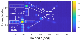
Figure 3: Example visualization of measured 60 GHz BRSRP data, with the LoS path and other landmarks being clearly visible. Antenna sidelobes are creating notable power spreading along the two axes.

Inspired by the structure of $\mathbf{B}$ in (8), let us consider its singular value decomposition (SVD), expressed as $\mathbf{B}=\mathbf{U}\mathbf{\Lambda}\mathbf{V}^{\top}$, where $\mathbf{U}\in\mathbb{R}^{L_{\textrm{TX}}\times L_{\textrm{TX}}}$, $\mathbf{V}\in\mathbb{R}^{L_{\textrm{RX}}\times L_{\textrm{RX}}}$ are unitary matrices, and $\mathbf{\Lambda}\in\mathbb{R}^{L_{\textrm{TX}}\times L_{\textrm{RX}}}$ is a rectangular diagonal matrix. In the main diagonal of $\mathbf{\Lambda}$, singular values of $\mathbf{B}$, $[\sigma_{1},\sigma_{2},...,,\sigma_{R}]>0$ are sorted in the descending order, where $R=\text{rank}(\mathbf{B})\leq\text{min}(L_{\textrm{TX}},L_{\textrm{RX}})$. The SVD can also be expressed as

$$\mathbf{B}=\sum_{r=1}^{R}\sigma_{r}\mathbf{u}_{r}\mathbf{v}_{r}^{\top}=\sum_{r=1}^{R}\mathbf{B}^{(1)}_{r},$$ (9)

where $\mathbf{u}_{r}$ and $\mathbf{v}_{r}$ are the $r^{\text{th}}$ columns of $\mathbf{U}$ and $\mathbf{V}$, respectively. Importantly, based on (8), $\mathbf{u}_{r}$ and $\mathbf{v}_{r}$ belong to the corresponding spans of $\{\mathbf{g}_{\text{TX}}(\boldsymbol{\psi}_{\text{TX},n})\}_{n=1}^{N}$ and $\{\mathbf{g}_{\text{RX}}(\boldsymbol{\psi}_{\text{RX},n})\}_{n=1}^{N}$. Thus, the $r^{\text{th}}$ singular vectors can be expressed as

$$\mathbf{u}_{r}\!=\!\!\sum_{n=1}^{N}\!q_{r,n}^{\text{u}}\mathbf{g}_{\text{TX}}(\boldsymbol{\psi}_{\text{TX},n})\text{ and }\mathbf{v}_{r}\!=\!\!\sum_{n=1}^{N}\!q_{r,n}^{\text{v}}\mathbf{g}_{\text{RX}}(\boldsymbol{\psi}_{\text{RX},n}),$$ (10)

where $q_{r,n}^{\text{u}}$ and $q_{r,n}^{\text{v}}$ are the linear combination weights of the spanning set vectors $\mathbf{g}_{\text{TX}}(\boldsymbol{\psi}_{\text{TX},n})$ and $\mathbf{g}_{\text{RX}}(\boldsymbol{\psi}_{\text{RX},n})$, respectively. In addition, $\mathbf{B}^{(1)}_{r}$ in (9) is a rank-1 matrix associated with the $r^{\text{th}}$ singular value and the related basis vectors $\mathbf{u}_{r}$ and $\mathbf{v}_{r}$. Furthermore, in the case of a sparse beamformed channel where all paths are well separated, the following holds

$$\begin{split}\mathbf{g}_{\text{TX}}(\boldsymbol{\psi}_{\text{TX},n})^{\top}\mathbf{g}_{\text{TX}}(\boldsymbol{\psi}_{\text{TX},n^{\prime}})&\approx\delta_{n-n^{\prime}}\text{ and}\\ \mathbf{g}_{\text{RX}}(\boldsymbol{\psi}_{\text{RX},n})^{\top}\mathbf{g}_{\text{RX}}(\boldsymbol{\psi}_{\text{RX},n^{\prime}})&\approx\delta_{n-n^{\prime}},\end{split}$$ (11)

where $\delta_{n-n^{\prime}}$ is a unit impulse function. In such case, each SVD term in (9) corresponds essentially to one propagation path, and thus $\mathbf{B}^{(1)}_{r}$ is a rank-1 approximation of the power map stemming from the corresponding path.

Interestingly, based on (8)–(10) and the corresponding fact that the singular vectors are in the span of the beam gain vectors, the SVD-based low-rank modeling approach can also inherently manage different unknown beam patterns, and is thus resilient to sidelobes and other beam pattern fluctuations. Specifically, the antenna sidelobes illustrated also in Fig. 3, can be decoupled from the peaks in $\mathbf{B}$ by using different low-rank approximations with increasing rank and analyzing the resulting power increment formed at each step. To this end, a pair of subsequent low-rank approximations of $\mathbf{B}$, denoted as $\mathbf{B}_{K-1}$ and $\mathbf{B}_{K}$, with $K<R$, can be expressed as

$$\mathbf{B}_{K}=\sum_{r=1}^{K}\sigma_{r}\mathbf{u}_{r}\mathbf{v}_{r}^{\top}=\sum_{r=1}^{K}\mathbf{B}^{(1)}_{r}=\mathbf{B}_{K-1}+\mathbf{B}^{(1)}_{K},\vspace{-1mm}$$ (12)

where the rank-1 matrix $\mathbf{B}^{(1)}_{K}=\sigma_{K}\mathbf{u}_{K}\mathbf{v}_{K}^{\top}$ represents a recovered BRSRP map increment between the two levels of approximation accuracy.

III-B2 Overall Approach and Refinements

Due to the relation of singular vectors to antenna response in (10) and the relation of the singular vectors and singular matrix in (9), the AoD and AoA estimates can be extracted recursively by processing rank-1 matrices $\mathbf{B}^{(1)}_{r}$ for separate singular values, while assuming only known TX beam angles $\{\Phi_{i}\}_{i=1}^{L_{\text{TX}}}$ and RX beam angles $\{\Theta_{j}\}_{j=1}^{L_{\text{RX}}}$. A suitable rank value for the low-rank approximation in (12) can be determined in various manner so that noise-dominated singular matrices are omitted from the approximation. In this article, we choose the approximation rank by ensuring that the low-rank approximation recovers a desired portion of the original total measured power, as described in Algorithm 1. Additionally, suitable rank selection can also help emphasizing LoS and single-bounce paths, over the corresponding multi-bounce paths [38] that are typically of low power.

Algorithm 1 Proposed AoD-AoA Extraction Algorithm

Input: TX beam angles $\{\Phi_{i}\}_{i=1}^{L_{\text{TX}}}$, RX beam angles $\{\Theta_{j}\}_{j=1}^{L_{\text{RX}}}$, power measurement matrix $\mathbf{B}\in\mathbb{R}^{L_{\text{TX}}\times L_{\text{RX}}}$, desired power ratio $p$, and power threshold $\beta_{th}$
Output: Number of estimated paths $\hat{N}$, AoD estimates $\{\hat{\phi}_{n}\}_{n=1}^{\hat{N}}$, and AoA estimates $\{\hat{\theta}_{n}\}_{n=1}^{\hat{N}}$

1:Compute SVD of BRSRP matrix: $\mathbf{B}=\mathbf{U}\mathbf{\Lambda}\mathbf{V}^{\top}$

2:Compute the total power $p_{\text{TOT}}=\sum_{r=1}^{R}\sigma_{r}^{2}$, where $\sigma_{r}$ is the $r^{\text{th}}$ singular value, and $R=\text{min}(L_{\textrm{TX}},L_{\textrm{RX}})$

3:Set $r=1$, $p_{r}=0$, $\mathcal{M}_{\text{est}}=\{\}$

4:while $p_{r}<p$ do

5:     Compute a rank-1 matrix: $\mathbf{B}^{(1)}_{r}=\sigma_{r}\mathbf{u}_{r}\mathbf{v}_{r}^{\top}$

6:     Find the indices of the element with maximum value:

7:         $(\hat{i}_{r},\hat{j}_{r})=\operatorname*{arg\,max}_{i,j}\mathbf{B}^{(1)}_{r}[i,j]$,

8:         where $\mathbf{B}^{(1)}_{r}[i,j]$ is the matrix $\mathbf{B}^{(1)}_{r}$ element at the

9:         $i^{\text{th}}$ row and $j^{\text{th}}$ column.

10:     Save the angles and power as a 3D set element:

11:         $\mathcal{M}_{\text{est}}\leftarrow\mathcal{M}_{\text{est}}\cup\{(\Phi_{\hat{i}_{r}},\Theta_{\hat{j}_{r}},\beta_{\hat{i}_{r},\hat{j}_{r}})\}$

12:     Compute the power ratio: $p_{r}\leftarrow\frac{1}{p_{\text{TOT}}}\sum_{\tilde{r}=1}^{r}\sigma_{\tilde{r}}^{2}$

13:     Set $r\leftarrow r+1$

14:end while, $K=r$

15:Power thresholding – choose only the components with power exceeding a given threshold:

16:         $\mathcal{M}_{\text{est}}\leftarrow\{\mathcal{M}_{\text{est}}\,|\,\text{elements with }\beta_{\hat{i}_{r},\hat{j}_{r}}\geq\beta_{th}\}$

17:Clustering – Perform clustering of elements in $\mathcal{M}_{\text{est}}$ to obtain $\hat{N}\leq K$ clusters $\mathcal{M}_{\text{est}}^{n}$, $n=1,\dots,\hat{N}$. For each cluster, angle estimates are obtained by computing a power-weighted cluster mean as $\bar{{\phi}}_{n}=(\sum_{s}\beta_{{\hat{i}_{s}},{\hat{j}_{s}}}{\Phi}_{\hat{i}_{s}})/\sum_{s}\beta_{{\hat{i}_{s}},{\hat{j}_{s}}}$ and $\bar{{\theta}}_{n}=(\sum_{s}\beta_{{\hat{i}_{s}},{\hat{j}_{s}}}{\Theta}_{\hat{i}_{s}})/\sum_{s}\beta_{{\hat{i}_{s}},{\hat{j}_{s}}}$, where the index $s$ is used to select elements from the specific cluster.

18:Polynomial fitting – a subset of the power matrix $\mathbf{B}$ around each cluster mean is fitted with a $2^{\text{nd}}$ degree polynomial surface. For the $n^{\text{th}}$ cluster, the final AoD and AoA estimates are found in closed form as a vertex of the local polynomial surface as $\hat{\phi}_{n}=(c_{5}c_{3}-2c_{6}c_{2})/(4c_{6}c_{4}-c_{5}^{2})$, $\hat{\theta}_{n}=(c_{5}c_{2}-2c_{4}c_{3})/(4c_{6}c_{4}-c_{5}^{2})$, where $c_{l},l=1...6$ are the coefficients of the polynomial surface.

The complete proposed procedure for obtaining AoD estimates $\{\hat{\phi}_{n}\}_{n=1}^{\hat{N}}$ and AoA estimates $\{\hat{\theta}_{n}\}_{n=1}^{\hat{N}}$ for $\hat{N}$ estimated paths, is stated and described in Algorithm 1. Besides the fundamental processing of rank-1 matrices for extracting angle information, three additional refinements are shown and applied, namely, power thresholding, clustering, and polynomial fitting. With power thresholding, we omit peaks which are close to noise level, and thus mitigate noise-related estimation errors. The clustering step, in turn, considers the fact that powerful peaks create large residuals and require more than one rank-1 singular matrix to be properly represented. Assuming spatially sparse channel, we expect such residual peaks to occur only in vicinity of powerful peaks that are spatially separated from each other, thus creating clusters in AoD-AoA domain. After the clustering step, where any existing clustering method [39] can be adopted, $\hat{N}$ clusters are obtained, whose cluster means represent the coarsely estimated AoD and AoA angles. Lastly, to enhance the angle estimation precision, each peak associated with a coarsely estimated AoD and AoA is fitted with a parabolic surface using a weighted least squares method. Fitting is performed within a local window of size approximately representing the beamwidth. The final AoD estimates $\{\hat{\phi}_{n}\}_{n=1}^{\hat{N}}$ and AoA estimates $\{\hat{\theta}_{n}\}_{n=1}^{\hat{N}}$ can be then found in closed form as a vertex of the parabolic surface for each peak.

Finally, we note that if paths share the same AoD, but have different AoAs, or vice versa, multiple paths can be represented by one rank-1 singular matrix. Thus, one could argue that the AoD-AoA extraction algorithm would benefit from multi-peak selection, however, with such measurement geometry, the weaker paths can be assumed as undesired multi-bounce paths in the considered SLAM setting.

III-B3 Complexity Assessment

The fundamental complexity order of the proposed SVD-based angle estimation method is $\mathcal{O}(\text{min}(L_{\textrm{TX}}L_{\textrm{RX}}^{2},L_{\textrm{TX}}^{2}L_{\textrm{RX}})+\text{min}(L_{\textrm{TX}},L_{\textrm{RX}})^{2}K+L_{\textrm{TX}}L_{\textrm{RX}}K)$, excluding further refinements of thresholding, clustering and polynomial fitting. The corresponding complexities of [15] as well as a classical cell-averaging constant false alarm rate (CFAR) detector [40], being used as benchmark methods along the numerical results, read $\mathcal{O}(\text{min}(L_{\textrm{TX}},L_{\textrm{RX}})^{3}+N_{\text{peak}}L_{\textrm{TX}}L_{\textrm{RX}})$, and $\mathcal{O}(L_{\textrm{TX}}L_{\textrm{RX}}N_{\text{TB}}^{2})$, respectively, where $N_{\text{peak}}$ is a maximum number of support squares and $N_{\text{TB}}$ is a size of the CFAR training window. For good performance, $N_{\text{TB}}^{2}$ is comparable to or larger than $L$ (i.e., $L_{\textrm{TX}}$ or $L_{\textrm{RX}}$), and thus all three methods have similar complexity order of $\mathcal{O}(L^{3})$.

III-C ToA Estimation

In general, the SS burst [34, 41] allows to establish the basic frame and OFDM symbol synchronization, however, PRS allows for larger bandwidth and thus facilitates more accurate symbol time estimation and particularly the fine ToA estimation. We thus next shortly address the ToA estimation, building on PRS and the corresponding PRS IDs [34, 41] – both known at the UE. The coarse ToA estimation is carried out using time-domain I/Q signals, already before the angle estimation phase, while the fine ToA estimation or refinement is carried out in frequency-domain only for the identified path angles. These together provide the estimates for the pathwise ToAs.

III-C1 Coarse ToA Estimation in Time Domain

First, sample-wise time delay estimation and beam ID search is performed by maximising the cross-correlation between the received waveform and potential reference waveforms in time domain. For sampling rate of $F_{s}$, we denote the $q^{\text{th}}$ time domain signal sample for the received signal and the PRS with PRS ID $\nu$ as $Y^{i,j}(q)$ and $X^{i,j}_{\nu}(q)$, respectively. Now, the estimated PRS ID $\hat{\nu}_{i,j}$ and sample-wise delay $\widehat{\Delta q}_{i,j}$ can be obtained as

$$(\hat{\nu}_{i,j},\widehat{\Delta q}_{i,j})=\operatorname*{arg\,max}_{\nu,\Delta q}\sum_{q=0}^{N_{\text{s}}-1}|Y^{i,j}[q+\Delta q]X^{i,j}_{\nu}[q]^{*}|^{2}.$$ (13)

Furthermore, the coarse delay estimate, defined with respect to the TX reference time, reads then $\hat{\tau}^{i,j}_{\text{c}}=\widehat{\Delta q}_{i,j}/F_{s}$.

III-C2 Fine ToA Estimation in Frequency Domain

The fine time delay estimation is performed per estimated path, using the frequency domain samples $y_{k,m}^{i,j}$ with $(k,m)\in\mathcal{M}_{RS}$, corresponding to the beam pair $(i,j)$ whose beam angles are closest to the estimated AoD and AoA. Such fine ToA estimate for path $n$, determined with respect to the beginning of the OFDM symbol, can be obtained as [42, Ch. 3.2]

$$\hat{\tau}_{\text{f},n}=\operatorname*{arg\,max}_{\tau}\left|\sum_{(k,m)\in\mathcal{M}_{RS}}(x_{k,m}^{\hat{i}_{n},\hat{j}_{n}})^{*}y_{k,m}^{\hat{i}_{n},\hat{j}_{n}}e^{j2\pi k\Delta f\tau}\right|,$$ (14)

where $\hat{i}_{n}=\operatorname*{arg\,min}_{i}(|\Phi_{i}-\hat{\phi}_{n}|)$ and $\hat{j}_{n}=\operatorname*{arg\,min}_{j}(|\Theta_{j}-\hat{\theta}_{n}|)$ are the TX and RX beam indices associated with the $n^{\text{th}}$ estimated path, respectively. In practice, (14) can be solved using an optimization algorithm, interpolated IFFT, or performing a brute force search over suitable propagation delays.

Finally, the complete ToA estimates are obtained as

$$\hat{\tau}_{n}=\hat{\tau}^{\hat{i}_{n},\hat{j}_{n}}_{\text{c}}+\hat{\tau}_{\text{f},n}$$ (15)

for path indices $n=1,\dots,\hat{N}$. As noted in [43, 41], the coarse ToA estimate can also be determined wrt. the frame start time. In such case, the possible excess time between the beginning of the frame and the actual RS transmission time can be taken into account in the coarse ToA estimate, while the path-wise fine ToA estimates remains intact. With unsynchronized TX and RX clocks, the ToA estimate in (15) is affected by the clock bias, as considered in Section IV.

IV Proposed Snapshot SLAM Method

Next, we describe the proposed snapshot SLAM method, building on the previously described AoA, AoD and ToA estimates. The fundamental problem geometry is illustrated in Fig. 2, while in the following, for clarity, we explicitly refer to BS and UE as the TX and RX entities, respectively.

IV-A Problem Formulation

It is assumed that the BS position and orientation, denoted with $[{\mathbf{p}}_{\textrm{BS}}^{\top},\,\alpha_{\textrm{BS}}]^{\top}$, are known while the unknown UE state is represented using the 2D position, heading and clock bias (cast in meters) as ${\mathbf{s}}=[{\mathbf{p}}_{\textrm{UE}}^{\top},\,\alpha_{\textrm{UE}},\,B_{\textrm{UE}}]^{\top}$. Furthermore, the $n$th single bounce propagation path is represented using the 2D interaction point or landmark ${\mathbf{m}}_{n}=[x_{n},\,y_{n}]^{\top}$, $n=2,3,...,\hat{N}$, where $\hat{N}$ denotes the number of the available AoA, AoD and ToA estimates in a given measurement location. For notational convenience, the LoS path index – if existing – is $n=1$.

In addition, let ${\mathbf{x}}_{n}=[{\mathbf{s}}^{\top},\,{\mathbf{m}}_{n}^{\top}]^{\top}$ denote the joint state of the UE and the $n$th landmark, ${\mathbf{m}}=[{\mathbf{m}}_{2}^{\top},\ldots,{\mathbf{m}}_{\hat{N}}^{\top}]^{\top}$ denotes the map which is the joint state of the $\hat{N}-1$ landmarks, and the unknown joint state of the UE and map is ${\mathbf{x}}=[{\mathbf{s}}^{\top},{\mathbf{m}}^{\top}]^{\top}$. Now, the estimation problem can be defined as

$$p({\mathbf{x}}\mid{\mathbf{z}})\propto p({\mathbf{x}})\prod_{n=1}^{\hat{N}}p({\mathbf{z}}_{n}\mid{\mathbf{x}}_{n}),$$ (16)

where $p({\mathbf{x}})=\mathcal{N}({\mathbf{x}}\mid\boldsymbol{\mu},\boldsymbol{\Sigma})$ is the prior for ${\mathbf{x}}$ obtained for example using external sensors or a previous estimate and $p({\mathbf{z}}_{n}\mid{\mathbf{x}}_{n})$ is the likelihood of the $n$th measurement. It is to be noted that typically snapshot SLAM implies that no prior information exists since the primary interest is analyzing what can be done with radio signals alone [16, 28] whereas in this article, we evaluate the system performance both with and without the prior. The measurements are defined as ${\mathbf{z}}_{n}=[c\hat{\tau}_{n},\,\hat{\phi}_{n},\,\hat{\theta}_{n}]^{\top}$ in which the delay estimates are converted to meters for convenience. An estimate for ${\mathbf{x}}$ can be obtained by maximizing (16), mathematically given by

$$\hat{{\mathbf{x}}}=\underset{{\mathbf{x}}}{\arg\max}\,p({\mathbf{x}}\mid{\mathbf{z}}).$$ (17)

Since the UE does not known whether the LoS exists or not, (17) is solved under NLoS only and under LoS +NLoS, separately. Propagation paths with distance to within one meter of the shortest path and power within $3\text{ dB}$ to the path with maximum power are considered as candidate LoS signals and $N_{\textrm{LoS}}$ denotes the number of LoS candidates. Furthermore, for each candidate, (17) is solved with and without a prior (see Section IV-D). This will give $2N_{\textrm{LoS}}+1$ solutions to (17) with different costs and the solution with lowest cost measured in terms of (21) can be selected as the estimate.

IV-B Measurement Models

Assuming that the measurement noise is zero-mean Gaussian, which is a common assumption is bistatic SLAM [14, 31], the likelihood function is Gaussian

$$p({\mathbf{z}}_{n}\mid{\mathbf{x}}_{n})=\mathcal{N}({\mathbf{z}}_{n}\mid{\mathbf{h}}_{n}({\mathbf{x}}),{\mathbf{R}}_{n}),$$ (18)

with mean ${\mathbf{h}}_{n}({\mathbf{x}})$ and covariance ${\mathbf{R}}_{n}$. Building on the geometry in Fig. 2, the mean is given by

$${\mathbf{h}}_{n}({\mathbf{x}})=\begin{bmatrix}d+B_{\textrm{UE}}\\ \textrm{atan}2(-\delta_{1,y},-\delta_{1,x})-\alpha_{\textrm{BS}}\\ \textrm{atan}2(\delta_{2,y},\delta_{2,x})-\alpha_{\textrm{UE}}\end{bmatrix}.$$ (19)

For the LoS path $(n=1)$, the parameters are defined as: $d=\lVert{\mathbf{p}}_{\textrm{BS}}-{\mathbf{p}}_{\textrm{UE}}\rVert$ and $[\delta_{1,x},\,\delta_{1,y}]^{\top}=[\delta_{2,x},\,\delta_{2,y}]^{\top}={\mathbf{p}}_{\textrm{BS}}-{\mathbf{p}}_{\textrm{UE}}$. Respectively for the $n$th NLoS path, the parameters are defined as: $d=\lVert{\mathbf{p}}_{\textrm{BS}}-{\mathbf{m}}_{n}\rVert+\lVert{\mathbf{m}}_{n}-{\mathbf{p}}_{\textrm{UE}}\rVert$, $[\delta_{1,x},\,\delta_{1,y}]^{\top}={\mathbf{p}}_{\textrm{BS}}-{\mathbf{m}}_{n}$ and $[\delta_{2,x},\,\delta_{2,y}]^{\top}={\mathbf{m}}_{n}-{\mathbf{p}}_{\textrm{UE}}$.

IV-C Regularized Robust Least Squares Estimator

Maximizing the posterior as given in (17), is equivalent to minimizing the negative log-likelihood

$$\hat{{\mathbf{x}}}=\underset{{\mathbf{x}}}{\arg\min}\,L({\mathbf{x}}),$$ (20)

in which $L({\mathbf{x}})$ is the objective function we wish to minimize. In this article, we utilize the following objective function

$$L({\mathbf{x}})=({\mathbf{x}}-\boldsymbol{\mu})^{\top}\boldsymbol{\Sigma}^{-1}({\mathbf{x}}-\boldsymbol{\mu})+\sum_{n=1}^{\hat{N}}f(q_{n}({\mathbf{x}})),$$ (21)

where the first term is a regularization term that encodes the prior information and the second term encodes the evidence provided by the measurements. In the second term, $f(\cdot)$ is a robust cost function which we will define later and

$$q_{n}({\mathbf{x}})=({\mathbf{z}}_{n}-{\mathbf{h}}_{n}({\mathbf{x}}))^{\top}{\mathbf{R}}_{n}^{-1}({\mathbf{z}}_{n}-{\mathbf{h}}_{n}({\mathbf{x}})).$$ (22)

defines a quadratic error.

The Gauss-Newton algorithm can be utilized to iteratively solve (21) and the method is based on approximating ${\mathbf{h}}_{n}({\mathbf{x}})$ using a first order Taylor series expansion [44], given by

$${\mathbf{h}}_{n}({\mathbf{x}})\approx{\mathbf{h}}_{n}(\hat{{\mathbf{x}}}^{(j)})+{\mathbf{J}}_{n}(\hat{{\mathbf{x}}}^{(j)})({\mathbf{x}}-\hat{{\mathbf{x}}}^{(j)}),$$ (23)

where $\hat{{\mathbf{x}}}^{(j)}$ is the estimate of ${\mathbf{x}}$ at the $j$th iteration and ${\mathbf{J}}_{n}(\hat{{\mathbf{x}}}^{(j)})=\nabla_{{\mathbf{x}}}{\mathbf{h}}_{n}({\mathbf{x}})|_{{\mathbf{x}}=\hat{{\mathbf{x}}}^{(j)}}$ is the Jacobian. The parameter update of the Gauss-Newton algorithm can be derived by plugging (23) into (21), setting the gradient of $L({\mathbf{x}})$ to zero and solving for ${\mathbf{x}}$, expressed as

$$\frac{\partial L({\mathbf{x}})}{\partial{\mathbf{x}}} =\frac{\partial}{\partial{\mathbf{x}}}({\mathbf{x}}-\boldsymbol{\mu})^{\top}\boldsymbol{\Sigma}^{-1}({\mathbf{x}}-\boldsymbol{\mu})+\sum_{n=1}^{\hat{N}}\frac{\partial f}{\partial q_{n}}\frac{\partial q_{n}}{\partial{\mathbf{x}}}$$ (24)

$$\approx 2\boldsymbol{\Sigma}^{-1}({\mathbf{x}}-\boldsymbol{\mu})-2\sum_{n=1}^{\hat{N}}{\mathbf{J}}_{n}^{\top}(\hat{{\mathbf{x}}}^{(j)})\tilde{{\mathbf{R}}}_{n}(\hat{{\mathbf{x}}}^{(j)})^{-1}$$

$$\quad\times\bigl{(}{\mathbf{z}}_{n}-{\mathbf{h}}_{n}(\hat{{\mathbf{x}}}^{(j)})-{\mathbf{J}}_{n}(\hat{{\mathbf{x}}}^{(j)})({\mathbf{x}}-\hat{{\mathbf{x}}}^{(j)})\bigr{)}=0,$$

in which

$$\tilde{{\mathbf{R}}}_{n}(\hat{{\mathbf{x}}}^{(j)})^{-1}=\frac{\partial f}{\partial q_{n}}\biggr{|}_{q_{n}=q_{n}(\hat{{\mathbf{x}}}^{(j)})}{\mathbf{R}}_{n}^{-1}.$$ (25)

We then set the next estimate $\hat{{\mathbf{x}}}^{(j+1)}$ to be equal to the minimum, which gives

$$\hat{{\mathbf{x}}}^{(j+1)} =\hat{{\mathbf{x}}}^{(j)}+{\mathbf{A}}^{-1}{\mathbf{b}},\quad\text{where}$$ (26)

$${\mathbf{A}} =\boldsymbol{\Sigma}^{-1}+\sum_{n=1}^{\hat{N}}{\mathbf{J}}_{n}^{\top}(\hat{{\mathbf{x}}}^{(j)})\tilde{{\mathbf{R}}}_{n}(\hat{{\mathbf{x}}}^{(j)})^{-1}{\mathbf{J}}_{n}(\hat{{\mathbf{x}}}^{(j)}),$$

$${\mathbf{b}} =\boldsymbol{\Sigma}^{-1}(\boldsymbol{\mu}-\hat{{\mathbf{x}}}^{(j)})$$

$$\quad+\sum_{n=1}^{\hat{N}}{\mathbf{J}}_{n}^{\top}(\hat{{\mathbf{x}}}^{(j)})\tilde{{\mathbf{R}}}_{n}(\hat{{\mathbf{x}}}^{(j)})^{-1}({\mathbf{z}}_{n}-{\mathbf{h}}_{n}(\hat{{\mathbf{x}}}^{(j)})).$$

In general, there are many possible robust cost functions that reduce the weight of components with large errors so that they have a smaller influence to the solution due to a reduced gradient [45]. In this article, we utilize the Cauchy cost function, $f(q_{n}({\mathbf{x}}))=\log(1+q_{n}({\mathbf{x}}))$, such that the second term of the objective function in (21) becomes

$$\sum_{n=1}^{\hat{N}}\log\left(1\mkern-4.0mu+\mkern-2.0mu({\mathbf{z}}_{n}-{\mathbf{h}}_{n}({\mathbf{x}}))^{\top}{\mathbf{R}}_{n}^{-1}({\mathbf{z}}_{n}-{\mathbf{h}}_{n}({\mathbf{x}}))\right)\mkern-4.0mu,$$ (27)

and the gradient is given by (24) in which

$$\tilde{{\mathbf{R}}}_{n}(\hat{{\mathbf{x}}}^{(j)})^{-1}=\frac{1}{1+q_{n}(\hat{{\mathbf{x}}}^{(j)})}{\mathbf{R}}_{n}^{-1}.$$ (28)

Thus, the new covariance matrix $\tilde{{\mathbf{R}}}_{n}$ is just an inflated version of the original covariance matrix ${\mathbf{R}}_{n}$, given by

$$\tilde{{\mathbf{R}}}_{n}(\hat{{\mathbf{x}}}^{(j)})\mkern-4.0mu=\mkern-4.0mu\left(1+({\mathbf{z}}_{n}\mkern-4.0mu-\mkern-2.0mu{\mathbf{h}}_{n}(\hat{{\mathbf{x}}}^{(j)}))^{\top}{\mathbf{R}}_{n}^{-1}({\mathbf{z}}_{n}\mkern-4.0mu-\mkern-2.0mu{\mathbf{h}}_{n}(\hat{{\mathbf{x}}}^{(j)}))\right){\mathbf{R}}_{n}$$ (29)

and it gets bigger as the quadratic error increases. As a consequence, cost terms that are very large and potential outliers are given less trust to diminish their impact.

In practice, taking a full step according to (26) might be too large with respect to the neighborhood for which the Taylor series approximation in (23) is valid. To avoid this, a scaled Gauss–Newton step can be done instead, proportional to the direction given by the local approximation. In this article, we use backtracking line search [46] to compute the step length. The resulting algorithm is summarized in Algorithm 2 and initialization of $\hat{{\mathbf{x}}}^{(0)}$ is presented in the following section.

Algorithm 2 Proposed Gauss-Newton algorithm

Input: Initial parameter guess $\hat{{\mathbf{x}}}^{(0)}$ and measurements ${\mathbf{z}}$
Output: Parameter estimate $\hat{{\mathbf{x}}}$ and covariance ${\mathbf{P}}$

1:Set $j\leftarrow 0$

2:repeat

3:     Calculate the update direction as given in (26):

4:         $\Delta\hat{{\mathbf{x}}}^{(j+1)}={\mathbf{A}}^{-1}{\mathbf{b}}$

5:     Compute step length $\gamma$ using Algorithm 9.2 in [46]

6:     Update parameter estimate:

7:         $\hat{{\mathbf{x}}}^{(j+1)}=\hat{{\mathbf{x}}}^{(j)}+\gamma\Delta\hat{{\mathbf{x}}}^{(j+1)}$

8:     Set $j\leftarrow j+1$

9:until Converged

10:$\hat{{\mathbf{x}}}=\hat{{\mathbf{x}}}^{(j)}$

11:${\mathbf{P}}=(\boldsymbol{\Sigma}^{-1}+\sum_{n=1}^{\hat{N}}{\mathbf{J}}_{n}^{\top}(\hat{{\mathbf{x}}}^{(j)})\tilde{{\mathbf{R}}}_{n}(\hat{{\mathbf{x}}}^{(j)})^{-1}{\mathbf{J}}_{n}(\hat{{\mathbf{x}}}^{(j)}))^{-1}$

IV-D Initialization

A major disadvantage of the Gauss–Newton approach is that the linearization of the measurement model is local. In highly nonlinear problems, this means that the solution can converge to a local minima and therefore, initialization of the algorithm is very important. To this end, let us define the prior mean and inverse of the covariance matrix as

$$\boldsymbol{\Sigma}^{-1} =\textrm{blkdiag}(\boldsymbol{\Sigma}_{{\mathbf{s}}{\mathbf{s}}}^{-1},\boldsymbol{\Sigma}_{{\mathbf{m}}_{2}{\mathbf{m}}_{2}}^{-1},\ldots,\boldsymbol{\Sigma}_{{\mathbf{m}}_{\hat{N}}{\mathbf{m}}_{\hat{N}}}^{-1}),$$ (30)

$$\boldsymbol{\mu} =[\boldsymbol{\mu}_{\mathbf{s}}^{\top},\,\boldsymbol{\mu}_{{\mathbf{m}}_{2}}^{\top},\,\ldots,\,\boldsymbol{\mu}_{{\mathbf{m}}_{\hat{N}}}^{\top}]^{\top},$$ (31)

where $\boldsymbol{\mu}_{{\mathbf{s}}}$, $\boldsymbol{\Sigma}_{{\mathbf{s}}{\mathbf{s}}}$, $\boldsymbol{\mu}_{{\mathbf{m}}_{n}}$ and $\boldsymbol{\Sigma}_{{\mathbf{m}}_{n}{\mathbf{m}}_{n}}$ denote the mean and covariance of the UE and $n$th map entry, respectively. Algorithm 2 is initialized using the prior mean, that is, $\hat{{\mathbf{x}}}^{(0)}=\boldsymbol{\mu}$.

Snapshot SLAM typically implies that no prior information exists $(\boldsymbol{\Sigma}^{-1}=\mathbf{0})$ [16, 28], whereas in this article, we evaluate the system performance both with and without the prior. If prior information is not available, the LoS must exist so that we can first compute a prior for the UE state as described in Section IV-D1 which can then be used to initialize the landmarks as presented in IV-D2. If a prior for the UE exists, the landmarks can be directly initialized using the prior as described in Section IV-D2. If a prior for the UE and map exists, Algorithm 2 can be directly initialized using the prior but in this article it is always assumed that no prior knowledge of the map is available, that is, $\boldsymbol{\Sigma}_{{\mathbf{m}}_{n}{\mathbf{m}}_{n}}^{-1}=\mathbf{0},\,n=2,\ldots,\hat{N}$.

IV-D1 UE Initialization Without Prior Information

The challenge in initializing the UE state using the LoS measurement is the unknown clock bias $B_{\textrm{UE}}$. One can consider different trial values of $B_{\textrm{UE}}$ over a range of $[{B}_{\textrm{UE,min}},\,{B}_{\textrm{UE,max}}]$ and for each trial value $\hat{B}_{\textrm{UE}}$, we form an augmented measurement $\check{{\mathbf{z}}}=[\hat{\tau}_{1},\,\hat{\phi}_{1},\,\hat{\theta}_{1},\,\hat{B}_{\textrm{UE}}]^{\top}$ and covariance $\check{{\mathbf{R}}}_{1}=\textrm{blkdiag}({\mathbf{R}}_{1},\sigma_{\hat{B}_{\textrm{UE}}}^{2})$, in which $\sigma_{\hat{B}_{\textrm{UE}}}^{2}$ is variance of the bias which is set higher than variance of the delay estimates. Then, the mean and covariance of the UE prior are given by

$$\boldsymbol{\mu}_{\mathbf{s}}=\check{{\mathbf{h}}}_{1}(\check{{\mathbf{z}}})\quad\text{and}\quad\boldsymbol{\Sigma}_{{\mathbf{s}}{\mathbf{s}}}=\check{{\mathbf{J}}}_{1}(\check{{\mathbf{z}}})\check{{\mathbf{R}}}_{1}\check{{\mathbf{J}}}_{1}(\check{{\mathbf{z}}})^{\top}$$ (32)

where $\check{{\mathbf{J}}}_{1}(\check{{\mathbf{z}}})$ denotes the Jacobian of $\check{{\mathbf{h}}}_{1}(\check{{\mathbf{z}}})$ evaluated with respect to $\check{{\mathbf{z}}}$ and the mean is defined as

$$\check{{\mathbf{h}}}_{1}(\tilde{{\mathbf{z}}})=[x_{\textrm{BS}}+\hat{x}_{1},\,y_{\textrm{BS}}+\hat{y}_{1},\,\textrm{atan}2(-\hat{y}_{1},-\hat{x}_{1})-\hat{\theta}_{1},\,\hat{B}_{\textrm{UE}}]^{\top}$$

in which $\hat{x}_{1}=(\hat{\tau}_{1}c-\hat{B}_{\textrm{UE}})\cos(\alpha_{\textrm{BS}}+\hat{\phi}_{1})$ and $\hat{y}_{1}=(\hat{\tau}_{1}c-\hat{B}_{\textrm{UE}})\sin(\alpha_{\textrm{BS}}+\hat{\phi}_{1})$. After computing the moments using (32), the landmark locations can be computed as presented in Section IV-D2. Then the trial with lowest cost according to (21), which also involves the landmarks, is selected as the UE prior. Due to computational reasons, we solve the described problem using constrained nonlinear optimization [46] for which the problem can be defined as

$$\hat{B}_{\textrm{UE}}=\underset{B_{\textrm{UE,min}}\leq B_{\textrm{UE}}\leq B_{\textrm{UE,max}}}{\arg\min}\,L({\mathbf{x}}),$$ (33)

with cost $L({\mathbf{x}})$ as given in (21).

IV-D2 Landmark Initialization

The affine approximation of the measurement likelihood in (18) around the UE prior reads

$$p({\mathbf{z}}_{n}\mid{\mathbf{x}}_{n})\approx\mathcal{N}({\mathbf{z}}_{n};{\mathbf{h}}_{n}({\mathbf{x}})+{\mathbf{J}}_{n}(\boldsymbol{\mu}_{\mathbf{s}})({\mathbf{s}}-\boldsymbol{\mu}_{\mathbf{s}}),{\mathbf{R}}_{n}),$$ (34)

where ${\mathbf{J}}_{n}(\boldsymbol{\mu}_{\mathbf{s}})=\nabla_{{\mathbf{s}}}{\mathbf{h}}_{n}({\mathbf{x}})|_{{\mathbf{s}}=\boldsymbol{\mu}_{\mathbf{s}}}$ is the Jacobian of ${\mathbf{h}}_{n}({\mathbf{x}})$ with respect to state ${\mathbf{s}}$ evaluated at $\boldsymbol{\mu}_{\mathbf{s}}$. Hence, the likelihood can be approximated as

$$p({\mathbf{z}}_{n}\mid{\mathbf{x}}_{n})\approx\mathcal{N}({\mathbf{z}}_{n};{\mathbf{h}}_{n}({\mathbf{x}}),{\mathbf{J}}_{n}(\boldsymbol{\mu}_{\mathbf{s}})\boldsymbol{\Sigma}_{{\mathbf{s}}{\mathbf{s}}}{\mathbf{J}}_{n}^{\top}(\boldsymbol{\mu}_{\mathbf{s}})+{\mathbf{R}}_{n}).$$ (35)

The $n$th map element is initialized by solving a nonlinear optimization problem, defined as

$$\boldsymbol{\mu}_{{\mathbf{m}}_{n}}=\underset{{\mathbf{m}}_{n}}{\textrm{arg\,min}}\,({\mathbf{z}}_{n}-{\mathbf{h}}_{n}({\mathbf{x}}))^{\top}{\mathbf{W}}_{n}^{-1}({\mathbf{z}}_{n}-{\mathbf{h}}_{n}({\mathbf{x}})),$$ (36)

where ${\mathbf{W}}_{n}={\mathbf{J}}_{n}(\boldsymbol{\mu}_{\mathbf{s}})\boldsymbol{\Sigma}_{{\mathbf{s}}{\mathbf{s}}}{\mathbf{J}}_{n}^{\top}(\boldsymbol{\mu}_{\mathbf{s}})+{\mathbf{R}}_{n}$. The optimization problem is initialized in a similar way as described in [14] and solved using the Gauss-Newton algorithm, with the exact details here omitted, as the algorithm is very similar to the one presented in Algorithm 2.

V Indoor Environment, Tools and Data

We consider a modern indoor environment at the Hervanta Campus of Tampere University, Finland, located in the so-called Campus Arena building. The environment is illustrated in terms of a floor plan and an actual photograph in Fig. 4, consisting of a fairly large partially open space containing a number of different landmarks such as columns, short walls, booths, and so forth. The BS is located in a narrow annex $3$m wide while the UE moves in the area with a trajectory shown in Fig. 4. Furthermore, $4\times 16$ planar antenna arrays are considered at both the transmitting and receiving ends, with azimuth 3 dB beamwidth of around 10^∘. Such antenna system assumption is certainly implementation feasible at BS end while for UEs the current mmWave implementations consider somewhat reduced antenna counts and thus broader beams. The considered PRS bandwidth is 400 MHz following [34].

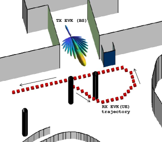
(a) Ray-tracing environment

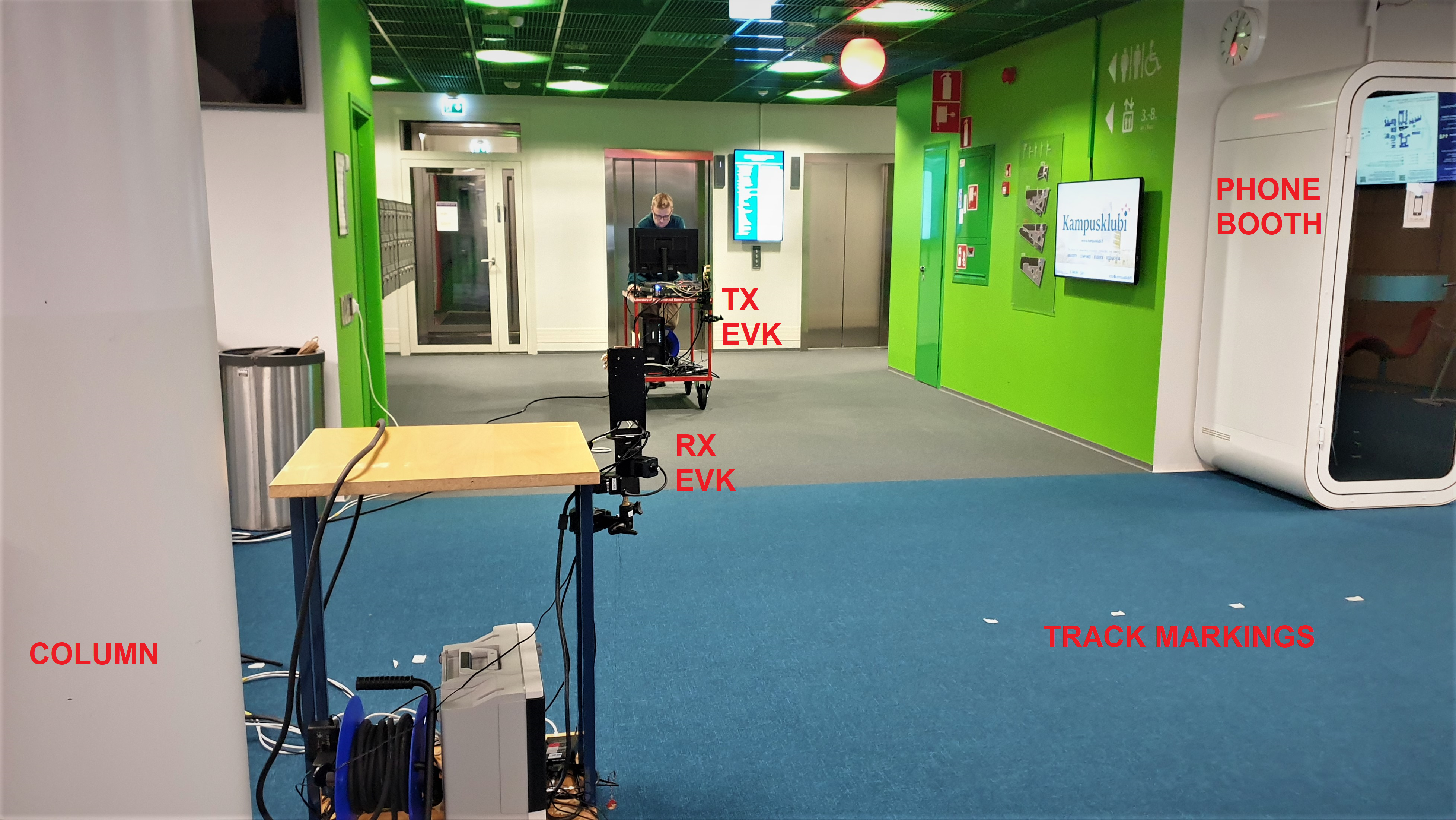
(b) Photograph of the physical measurement environment

Figure 4: Illustrations of the considered indoor environment. (a) Ray-tracing model visualization showing the TX/BS position and the RX/UE trajectory; (b) Photograph from the physical premises with the TX and RX trolleys also shown during the measurement campaign.

V-A Ray Tracing Tool and Assumptions

To carry out evaluations with well-defined and known ground-truth, ray tracing was performed with Wireless InSite^® [47]. The true physical environment is reproduced using the indoor floor plan editor fitted to the building blueprint, while noting also accurately different movable entities and objects such as an indoor phone booth. The ITU $60$ GHz material models [48], namely, layered drywall, wood, glass, floor and ceiling board were used. The BS position and UE trajectory consisting of $45$ points $0.5$m apart are accurately matched to those used in the actual measurements. Omnidirectional antennas were used for the ray casting, and the reception with path elevation was limited to $80^{\circ}-100^{\circ}$, reflecting essentially the azimuth plane. Furthermore, ray casting was limited to $25$ rays per UE position, and the number of material interactions to four reflections and one diffraction. The ray-tracing model considers specular reflection (SR) and diffraction (D), such that an unambiguous ground truth for the performance assessment of the proposed and benchmark angle estimation methods can be obtained.

The ray-tracing model is further combined with I/Q waveform processing in Matlab, such that realistic received I/Q samples can be generated, per UE location. Here, the TX and RX beampatterns are modelled through classical matched filter type responses where the beamforming weights are matched to the corresponding steering vector of the beamforming angle. Additionally, we allow for similar mechanical rotation patterns as in the actual measurements in order to cover $180^{\circ}$ field-of-view (FoV) in TX and $360^{\circ}$ FoV in RX (for further details, see the following subsection). These together facilitate a maximum of $L_{\textrm{TX}}$ = 126 and $L_{\textrm{RX}}$ = 252 beams at TX and RX, respectively. Moreover, we model accurately the signal-to-noise ratio (SNR) characteristics of the environment such that the prevailing SNR at each UE/RX point is adjusted according to the actual SNR observed in the corresponding physical RF measurements.

V-B Measurement Setup and Data

In the actual mmWave measurements, Sivers Semiconductors Evaluation Kits EVK06002 [49] were used as the TX and RX entities. The overall operational band of EVK06002 is $57-71$ GHz, and it consists of strip antenna elements arranged in $4\times 16$ arrays for each polarization, integrated with the electrical phase and amplitude control of the individual elements. The TX EVK was connected to a PC-controlled Arbitrary Waveform Generator M8195A, whereas the RX EVK was connected to the Keysight DSOS804A oscilloscope, which serve as data conversion interfaces towards digital signal processing. Similar to the ray-tracing case, the transmitted PRS-carrying I/Q waveforms were created using the Matlab 5G Toolbox including also embedding of different PRS IDs.

The beamforming capabilities of the Sivers EVK allows for synthesizing electrically controlled beams, building on embedded proprietary codebook. The exact beampatterns are unknown but based on elementary antenna measurements resemble those of the ray tracing model complemented with additional tapering. Since the electrical beamforming FoV of the EVK is limited to $[-45^{\circ},45^{\circ}]$, both TX and RX EVK were complemented with FLIR Pan Tilt PTU-46 for additional mechanical rotation capabilities, in order to cover $180^{\circ}$ and $360^{\circ}$ FoVs with maximum of $L_{\textrm{TX}}$ = 126 and $L_{\textrm{RX}}$ = 252 TX and RX beams, respectively. Both receiver and transmitter were controlled by the same PC and synchronized to the same clock via a coaxial cable to provide a reference for ToA measurements. Additionally, the true UE locations were recorded accurately for ground-truth purposes. The measurement setup and a glimpse of the physical environment are shown along the Fig. 4.

The complete 60 GHz I/Q measurement data set as well as the corresponding processed channel parameter data set, together with supportive scripts are all openly shared along the final published article.

VI Results

In this section, the angle estimation results as well as the complete end-to-end SLAM results are presented and analyzed. The angle estimator assessment builds on the ray tracing data, as it contains the ground-truth information also for the landmarks. The end-to-end SLAM assessment, in turn, builds on the true measurement data.

VI-A Angle Extraction Results with Ray Tracing Data

The performance of the proposed SVD-based method is assessed and compared to the available successive cancellation-based reference method described in [15]. Additionally, the classical CFAR detector [40] is also implemented and considered as an additional benchmark solution, as such is widely used, e.g., in radar context for target detection subject to clutter.

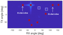
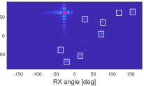
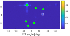
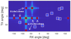
(a) a

(b) b

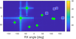
(c) c

Figure 5: Illustration of angle extraction methods in NLoS (upper row) and LoS (lower row) UE locations. (a) Cancellation method [15] for $N_{\text{peaks}}=10$, $\epsilon=0.05$ (NLoS) and $0.1$ (LoS); (b) CFAR [40] for $N_{\text{TB}}=15$ and $P_{\text{FA}}=0.002$ (NLoS) and $0.12$ (LoS); (c) Proposed SVD method for $p$ of $99.9\%$ (NLoS) and $99.99\%$ (LoS). Extracted path angles are marked with colored dots, side-lobe false detections with arrows, and missed detections with squares.

The method in [15] is parameterised with the so-called support power increment, $\epsilon$, and the maximum number of searched peaks, $N_{\text{peaks}}$. We additionally apply power thresholding to reduce the amount of false detections, and thereon to have as fair comparison as possible. The CFAR technique, in turn, uses training cells of size $N_{\text{TB}}$ around the target cell to estimate the local noise level to reach the given false alarm probability $P_{\text{FA}}$. The Matlab 2D CFAR detector implementation from phased array system toolbox was used, while further clustering was also applied to the results as CFAR method yields easily multiple AoD-AoA estimates per one peak.

VI-A1 Qualitative Comparison

The capabilities of the different methods are first visually illustrated in Fig. 5, covering both NLoS and LoS UE locations, and with the parametrizations as shown in the caption. As can be observed, the method from [15] has notable challenges in dealing with antenna sidelobes, while also several true propagation paths are missed especially in LoS case. The CFAR has also clear limitations with sidelobes while missing a large number of true landmarks in NLoS. The proposed method, in turn, is able to offer enhanced performance in both NLoS and LoS, while processing efficiently also the antenna sidelobes.

(a) a

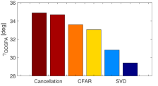
(b) b

(c) c

Figure 6: Quantitative assessment of different angle extraction methods. (a) GOSPA metric at different UE/RX locations for cancellation-based method [15] with $\epsilon=0.1$ ( ) and $\epsilon=0.05$ ( ), for CFAR method [40] with $P_{\text{FA}}=0.12$ ( ) and $P_{\text{FA}}=0.002$ ( ), and for the proposed SVD-based method with $p=99.9\%$ ( ) and $p=99.99\%$ ( ). (b) Corresponding average GOSPA metrics for all methods. (c) Average sidelobe detection metric for all methods.

VI-A2 Quantitative Comparison

As illustrated in Fig. 5, the amounts of the detected paths differ from method to another, while the ray-tracing model limits the amount of ground-truth paths to the earlier noted number of 25. Such data of different cardinality can be reliably compared and quantitatively assessed using the generalized optimal sub-pattern assignment (GOSPA) metric [50], which takes into account, in addition to root-mean-squared errors (RMSEs) of the quantities of interest, the numbers of false detection, $N_{\text{FD}}$, and missed detection, $N_{\text{MD}}$. We thus utilize the GOSPA metric for quantitative assessment, and express it in degrees as $\gamma_{\text{GOSPA}}=(\gamma_{\text{RMSE}}+(N_{\text{FD}}+N_{\text{MD}})d_{c}^{\mathcal{P}}/\alpha)^{(1/\mathcal{P})}$, where the parameters $d_{c}=10^{\circ}$, $\mathcal{P}=2$ and $\alpha=2$ are cutoff distance, exponent power and cardinality penalty factor, respectively.

Furthermore, a subset of all false detections are due to the sidelobes. Such sidelobe effects, unlike those of a noise, cannot be reduced by increasing the number of observations. Thus, we consider sidelobe false detection (SLFD) a systematic error that is especially detrimental to the performance of the whole end-to-end system. To this end, we introduce an additional metric that quantifies the number of SLFDs, $N_{\text{SLFD}}$. We specifically express the SLFD through the following conditions of (i) the ToA estimates are within a threshold of $|\hat{\tau}_{n_{1}}-\hat{\tau}_{n_{2}}|\leq\tau_{\text{th}}$, and (ii) the corresponding TX or RX beam indices differ at most by one, i.e., $(|\hat{i}_{n_{1}}-\hat{i}_{n_{2}}|\leq 1)\lor(|\hat{j}_{n_{1}}-\hat{j}_{n_{2}}|\leq 1)$. A tight delay threshold of $\tau_{\text{th}}=0.3\,\text{ns}$ is used in the numerical assessment. Finally, to present the sidelobe detection metric comparable to GOSPA, the same penalty factor is used, and thus the final metric is expressed as $\gamma_{\text{SLFD}}=\left((N_{\text{SLFD}}d_{c}^{\mathcal{P}})/\alpha\right)^{(1/\mathcal{P})}$.

The quantitative comparison between the three methods in terms of GOSPA and sidelobe detection metric are presented in Fig. 6, covering the whole UE/RX trajectory shown in Fig. 4, while also noting the options for the different parametrizations. In terms of the GOSPA metric, the proposed SVD-based method clearly outperforms the reference methods. Additionally, in terms of the SLFD metric, the proposed method outperforms that in [15] by a large margin. The CFAR with $P_{\text{FA}}=0.002$ is closer in performance, however, having clear challenges to detect the actual multipaths as shown in Fig. 5 already.

In summary, the proposed SVD approach outperforms the prior-art benchmark methods. As demonstrated by the ray-tracing results, it offers robust performance in both LoS and NLoS scenarios, while is also having built-in mechanism to suppress the impacts of the unavoidable antenna sidelobes.

VI-B SLAM Results with Measurement Data

(a) BM1 [28]

(b) BM2 [31]

(c) Proposed SLAM approach

Figure 7: Visual illustration of the performance of the different SLAM algorithms with measurement data including UE clock bias. In the figures, location of the BS illustrated using ( ), the ground truth UE trajectory with ( ), the UE position estimates using ( ) and the estimated landmark locations with ( ).

Next, the actual end-to-end SLAM results are provided and analyzed, utilizing the true measurement data. We use the proposed SVD method for angle estimation, and assume $p=99.9\%$. The ToA estimation is carried out as described in (13)–(15), while using brute force search to solve (14)

The proposed SLAM method is benchmarked with respect to two other SLAM approaches [28, 31]. The first benchmark is a geometry based snapshot SLAM algorithm [28] referred to as BM1 and the second is a recursive probability hypothesis density (PHD)-SLAM filter [31] referred to as BM2. In the following, the time delay and clock bias are converted to distance for convenience, and the clock bias is emulated to evolve according to a random walk model with variance $\sigma_{B}^{2}=1\,\textrm{m}^{2}$. The measurement noise covariance used in the experiments is ${\mathbf{R}}_{n}=\textrm{diag}([0.3\,\textrm{m},\;3\,\textrm{deg},\;3\,\textrm{deg}]^{2}),\,\forall\,n$. The mean and covariance of the UE prior for the proposed method are $\boldsymbol{\mu}_{\mathbf{s}}=\boldsymbol{\mu}_{{\mathbf{s}},\textrm{prev}}$ and $\boldsymbol{\Sigma}_{{\mathbf{s}}{\mathbf{s}}}=\mathbf{I}_{4}$, in which $\boldsymbol{\mu}_{{\mathbf{s}},\textrm{prev}}$ denotes the UE state estimate at the previous measurement position. In the first measurement position, which is located at $[0.55,\,-2.75]^{\top}$, there is no prior and estimation is possible because the LoS signal exists. The PHD-SLAM filter is implemented using $1000$ particles, the UE state is modeled to evolve according to a random walk model and the process noise is set to ${\mathbf{Q}}=\mathbf{I}_{4}$ which is the same as covariance of the UE prior. The PHD-SLAM filter is initialized using the proposed snapshot SLAM algorithm. Since BM1 is sensitive to outliers, measurements labeled as outliers are removed from the data for BM1 unless otherwise stated.

VI-B1 Qualitative Comparison

The example mapping and localization performance of the algorithms are visualized in Fig. 7. Qualitative analysis indicates that the map and UE position estimates are more accurate with BM2 and the proposed SLAM algorithm than with BM1. For BM1, the estimate is close to the ground truth and the estimated landmark locations are inline with the map in many measurement positions. In several locations however, the estimates are very inaccurate and there are two primary reasons for this. First of all, the method requires four NLoS signals so that the system is identifiable and this criterion is not satisfied at every measurement position. For example, when the UE is located at ${\mathbf{p}}_{\textrm{UE}}=[-5.5,\,-2.3]^{\top}$, there are only three propagation paths meaning that the system is underdetermined resulting in an inaccurate estimates as illustrated in Fig. 7. The second reason is that in several measurement positions, the cost function of BM1 is multimodal and the global minima is not the one closest to the ground truth. The proposed method and BM2 can operate in mixed LoS/NLoS conditions and the prior or posterior from the previous time step can be viewed as a regularization term which constrains the posterior update so that the system state is identifiable at every measurement position. Moreover, the resulting estimates for BM2 and the proposed method can be viewed as a weighted average of the evidence provided by the data and the regularization term. Thus, the estimate is expected to be close to the ground truth as long as the prior is not biased and the covariance captures the underlying uncertainties correctly. Lastly, both BM2 and the proposed approach result in sufficient SLAM performance despite the measurement data being corrupted by outliers as shown in Fig. 7.

VI-B2 Quantitative Comparison

TABLE I: Performance summary of the different estimators

Estimator	Position [m]	Heading [deg]	Bias [m]	Time [s]
BM1	$1.70\pm 1.36$	$29.17\pm 28.98$	$1.85\pm 1.86$	$13.43$
BM2∗	$1.51\pm 1.23$	$14.26\pm 14.16$	$0.92\pm 0.86$	$1.39$
BM2	$0.55\pm 0.23$	$2.56\pm 2.45$	$0.46\pm 0.40$	$141.12$
Proposed	$0.55\pm 0.32$	$2.26\pm 2.18$	$0.52\pm 0.50$	$1.60$
*The PHD-SLAM filter is implemented with $10$ particles.

The algorithms are next evaluated quantitatively while since the ground truth landmark locations are unknown, the mapping accuracy is excluded which a common practice in SLAM when using experimental data. The performance metrics are tabulated in Table I in which the position, heading and bias errors are computed using the RMSE and standard deviation (STD). Even without outliers, BM1 results in unsatisfactory performance due to the reason discussed above. The other two methods outperform BM1 and have comparative performance among each other. However, the computational complexity of BM2 is two orders of magnitude higher than with the proposed method. One could decrease the computational complexity by using less particles (see BM2^∗ in Table I) but at the same time, the accuracy of the filter degrades notably. Thus, a major advantage of the proposed method is that it combines high accuracy together with low computational overhead.

Figure 8: Position RMSEs of different algorithms in LoS and NLoS conditions with UE clock bias, and with ( ) and without ( ) outliers. The heading and bias RMSE have a similar trend but are omitted from the figure for brevity. The impact of the different objective function variants in (21) are also shown, including i) OFv0: no prior and quadratic cost function; ii) OFv1: no prior and robust cost function; and iii) OFv2: prior and quadratic cost function.

Next, we evaluate the different algorithms with and without outliers, and in LoS and NLoS conditions. The results are summarized in Fig. 8 and in general, the accuracy of all methods is better when the LoS is available. The performance of BM1 degrades significantly if the data contains outliers, whereas the performance of BM2 and the proposed method only degrade slightly. This indicates that both methods are capable of handling noisy measurements that are not inline with the models. The mechanisms how the two methods deal with outliers are quite different. The PHD-SLAM filter associates the outliers to clutter so that they do not affect the UE estimate, whereas the proposed method inflates the covariance according to (29) such that outliers are given less trust thus diminishing their impact. Interestingly, the proposed method outperforms BM2 in LoS conditions and vice versa in NLoS conditions. For the proposed method and when the LoS signal exists, the hypothesis that minimizes the cost function is typically the one for which the prior is computed using the LoS and the estimate is computed only from the evidence provided by the data. In this particular scenario, in which the prior uncertainty and the process noise of the dynamic model used by BM2 are high, relying solely on the measurements is beneficial. In NLoS conditions and when the proposed method cannot be initialized using the measurements, filtering is beneficial and BM2 outperforms the proposed method – however, at the expense of substantially higher complexity.

Lastly, we decompose the objective function of the proposed method and analyze the performance impact of the prior and the robust cost function. The results are illustrated in Fig. 8 from which we can conclude the following: (i) Without prior information and using a quadratic cost function (OFv0), the SLAM solution is useless in NLoS conditions and/or when the data contains outliers. The method outperforms BM1 only if the outliers are removed from the data and if the LoS signal exists. (ii) Without prior information and using a robust cost function (OFv1), the estimator yields comparative performance as the proposed method in LoS conditions, whereas in NLoS conditions the estimates are very innaccurate. (iii) With prior information and using a quadratic cost function (OFv2), the results are comparative to BM1 in both LoS and NLoS conditions and the performance improves significantly if the outliers are removed from the data. Thus to conclude, the robust cost function is a strict requirement of snapshot SLAM algorithms that are utilized in realistic scenarios in which the measurements are noisy and contain outliers. Moreover, prior information is required to improve identifiability of the system and enable estimation in mixed LoS/NLoS conditions.

VII Conclusions

In this article, we addressed the timely notion of mmWave radio SLAM from end-to-end processing perspective. We first proposed a novel SVD-based estimation approach for acquiring the AoAs and AoDs of the involved propagation paths. The method operates on BRSRP measurements and does not need information of the antenna system beampatterns or the involved beamformers, while offering built-in robustness against antenna sidelobes. Secondly, a new snapshot SLAM method was also proposed, to jointly estimate the locations of the landmarks and the UE, offering improved robustness and identifiability compared to prior-art. The performance of the proposed methods was comprehensively assessed through ray tracing and true measurement data at 60 GHz. The results show that the methods outperform the relevant prior-art, with the end-to-end performance being comparable or even better compared to sequential filtering solutions while offering substantially reduced complexity. Finally, we provide the measured 60 GHz data openly available for the research community. Our future work considers extending the proposed angle estimation methods to include multi-bounce detection and estimation with rank-1 singular matrices, thus facilitating further evolved SLAM solutions beyond the common single-bounce approaches.

Proof of Lemma 1

We first denote $\zeta_{k,m,n}^{i,j}=x_{k,m}^{i,j}e^{-\mathrm{i}2\pi k\Delta f\tau_{n}}e^{\mathrm{i}2\pi mT_{\text{sym}}f_{\text{D},n}}$ and $\tilde{G}_{n}^{i,j}=\xi_{n}G_{\text{TX},i}(\boldsymbol{\psi}_{\text{TX},n})G_{\text{RX},j}(\boldsymbol{\psi}_{\text{RX},n})$. Now, by substituting (3) into (4), the BRSRP measurement can be written as

$$\begin{split}\beta_{i,j}\!&=\!\frac{1}{{N}_{\text{RS}}}\!\!\sum_{\begin{subarray}{c}(k,m)\\ \in\mathcal{M}_{\text{RS}}\end{subarray}}\!\!\Bigg{\{}\Big{|}\sum_{n=1}^{N}\tilde{G}_{n}^{i,j}\zeta_{k,m,n}^{i,j}\Big{|}^{2}+\Big{|}\tilde{n}_{k,m}^{i,j}\Big{|}^{2}\\[-7.0pt] &\mspace{25.0mu}+2\mathfrak{Re}\Big{[}\left(\tilde{n}_{k,m}^{i,j}\right)^{*}\sum_{n=1}^{N}\tilde{G}_{n}^{i,j}\zeta_{k,m,n}^{i,j}\Big{]}\Bigg{\}}\\ &=\!\frac{1}{{N}_{\text{RS}}}\!\!\sum_{\begin{subarray}{c}(k,m)\\ \in\mathcal{M}_{\text{RS}}\end{subarray}}\Big{\{}\!\!\sum_{n=1}^{N}\Big{|}\tilde{G}_{n}^{i,j}\zeta_{k,m,n}^{i,j}\Big{|}^{2}+\Big{|}\tilde{n}_{k,m}^{i,j}\Big{|}^{2}\Big{\}}\\[-6.0pt] &+\overbrace{\frac{2}{{N}_{\text{RS}}}\!\!\!\sum_{\begin{subarray}{c}(k,m)\\ \in\mathcal{M}_{\text{RS}}\end{subarray}}\!\!\!\mathfrak{Re}\!\Big{[}\!\left(\tilde{n}_{k,m}^{i,j}\right)^{*}\sum_{n=1}^{N}\tilde{G}_{n}^{i,j}\zeta_{k,m,n}^{i,j}\Big{]}}^{\hskip 56.9055pt\text{Noise cross terms denoted as }S_{\text{noise}}\approx 0}\\[-7.0pt] &+\overbrace{\frac{2}{{N}_{\text{RS}}}\!\!\!\sum_{\begin{subarray}{c}(k,m)\\ \in\mathcal{M}_{\text{RS}}\end{subarray}}\!\!\!\mathfrak{Re}\!\Big{[}\!\sum_{n_{1}=1}^{N}\!\!\sum_{\begin{subarray}{c}n_{2}=1\\ n_{2}>n_{1}\end{subarray}}^{N}\!\!(\tilde{G}_{n_{1}}^{i,j}\zeta_{k,m,n_{1}}^{i,j})^{*}\tilde{G}_{n_{2}}^{i,j}\zeta_{k,m,n_{2}}^{i,j}\Big{]}}^{\hskip 28.45274pt\text{Squaring cross terms denoted as }S_{\text{sq}}\approx 0}\end{split}$$

The expected value of the noise cross terms equals to zero, and thus $S_{\text{noise}}\rightarrow 0$ when increasing $K$ and/or $M$. By rearranging summation order, the squaring cross terms can be rewritten as

$$S_{\text{sq}}=\!\!\frac{2}{{N}_{\text{RS}}}\!\mathfrak{Re}\Big{[}\!\sum_{n_{1}=1}^{N}\!\!\sum_{\begin{subarray}{c}n_{2}=1\\ n_{2}>n_{1}\end{subarray}}^{N}\!\!\!(\tilde{G}_{n_{1}}^{i,j})^{*}\tilde{G}_{n_{2}}^{i,j}\!\!\!\sum_{\begin{subarray}{c}(k,m)\\ \in\mathcal{M}_{\text{RS}}\end{subarray}}\!\!\!(\zeta_{k,m,n_{1}}^{i,j})^{*}\zeta_{k,m,n_{2}}^{i,j}\Big{]}.\vspace{-6pt}$$

Now, considering $|x_{k,m}^{i,j}|\!\!=\!\!1$ and using (5), $\sum_{(k,m)\in\mathcal{M}_{\text{RS}}}\!(\zeta_{k,m,n_{1}}^{i,j})^{*}\zeta_{k,m,n_{2}}^{i,j}\!\!\!=\!\!\mathbf{b}_{n_{1}}^{\mathrm{H}}\mathbf{b}_{n_{2}}\mathbf{c}_{n_{1}}^{\mathrm{H}}\mathbf{c}_{n_{2}}\!\approx\!0$. Finally, as $|\zeta_{k,m,n}^{i,j}|=1\,\forall k,m$, the BRSRP measurement can be formulated as given in (6).

References

- [1] L. Xie, et al., “Collaborative sensing in perceptive mobile networks: Opportunities and challenges,” IEEE Wireless Commun., vol. 30, no. 1, pp. 16–23, 2023.
- [2] O. Kanhere et al., “Position Location for Futuristic Cellular Communications: 5G and Beyond,” IEEE Commun. Mag., vol. 59, no. 1, pp. 70–75, 2021.
- [3] ITU-R, “Future technology trends of terrestrial International Mobile Telecommunications systems towards 2030 and beyond,” Tech. Rep. M.2516-0, Nov. 2022.
- [4] H. Tataria et al., “6G wireless systems: Vision, requirements, challenges, insights, and opportunities,” Proceedings of the IEEE, vol. 109, no. 7, pp. 1166–1199, 2021.
- [5] F. Liu et al., “Integrated sensing and communications: Toward dual-functional wireless networks for 6G and beyond,” IEEE J. Select. Areas Commun., vol. 40, no. 6, pp. 1728–1767, 2022.
- [6] J. Talvitie, et al., “Orientation and location tracking of XR devices: 5G carrier phase-based methods,” IEEE J. Select. Topics Signal Process., pp. 1–16, 2023.
- [7] M. Koivisto et al., “Joint device positioning and clock synchronization in 5G ultra-dense networks,” IEEE Trans. Wireless Commun., vol. 16, no. 5, pp. 2866–2881, 2017.
- [8] Y. Lu et al., “Bayesian filtering for joint multi-user positioning, synchronization and anchor state calibration,” IEEE Trans. Veh. Technol., vol. 72, no. 8, pp. 10 949–10 964, 2023.
- [9] R. Mendrzik, et al., “Enabling situational awareness in millimeter wave massive MIMO systems,” IEEE J. Select. Topics Signal Process., vol. 13, no. 5, pp. 1196–1211, Sept. 2019.
- [10] H. Que et al., “Joint beam management and SLAM for mmWave communication systems,” IEEE Trans. Commun., 2023.
- [11] 3GPP TS 38.104, “NR; Base Station (BS) radio transmission and reception, Rel. 18,” V18.3.0, Sept. 2023.
- [12] W. Saad, et al., “A vision of 6G wireless systems: Applications, trends, technologies, and open research problems,” IEEE Network, vol. 34, no. 3, pp. 134–142, 2020.
- [13] Y. Ge et al., “A computationally efficient EK-PMBM filter for bistatic mmWave radio SLAM,” IEEE J. Select. Areas Commun., vol. 40, no. 7, pp. 2179–2192, 2022.
- [14] H. Kim et al., “5G mmWave cooperative positioning and mapping using multi-model PHD filter and map fusion,” IEEE Trans. Wireless Commun., vol. 19, no. 6, pp. 3782–3795, 2020.
- [15] J. Yang et al., “Angle-based SLAM on 5G mmWave systems: Design, implementation, and measurement,” IEEE Internet of Things J., pp. 1–17, 2023.
- [16] A. Shahmansoori, et al., “Position and orientation estimation through millimeter-wave MIMO in 5G systems,” IEEE Trans. Wireless Commun., vol. 17, no. 3, pp. 1822–1835, 2018.
- [17] J. Salmi, et al., “Detection and tracking of MIMO propagation path parameters using state-space approach,” IEEE Trans. Signal Process., vol. 57, no. 4, pp. 1538–1550, 2009.
- [18] T. Jost, et al., “Detection and tracking of mobile propagation channel paths,” IEEE Trans. Antennas Propagat., vol. 60, no. 10, pp. 4875–4883, 2012.
- [19] A. Alkhateeb, et al., “Channel estimation and hybrid precoding for millimeter wave cellular systems,” IEEE J. Select. Topics Signal Process., vol. 8, no. 5, pp. 831–846, 2014.
- [20] C. Qin, et al., “Angle-of-arrival acquisition and tracking via virtual subarrays in an analog array,” in Proc. IEEE VTC-Fall, 2019, pp. 1–5.
- [21] A. Tulino, et al., “Parametrical channel estimation in mmWave using atomic norm,” in Proc. IEEE GLOBECOM, 2022.
- [22] M. Sánchez-Fernández, et al., “Gridless multidimensional angle-of-arrival estimation for arbitrary 3D antenna arrays,” IEEE Trans. Wireless Commun., vol. 20, no. 7, pp. 4748–4764, 2021.
- [23] D. Zhu, et al., “Two-dimensional AoD and AoA acquisition for wideband millimeter-wave systems with dual-polarized MIMO,” IEEE Trans. Wireless Commun., vol. 16, no. 12, pp. 7890–7905, 2017.
- [24] V. Boljanovic et al., “Fast beam training with true-time-delay arrays in wideband millimeter-wave systems,” IEEE Trans. Circuits Syst. I, vol. 68, no. 4, pp. 1727–1739, 2021.
- [25] ——, “Joint millimeter-wave AoD and AoA estimation using one OFDM symbol and frequency-dependent beams,” in Proc. IEEE ICASSP, 2023.
- [26] P. Gu, et al., “Channel estimation of mmWave massive MIMO system based on manifold learning,” in Proc. IEEE ICCT, 2022.
- [27] H. Wymeersch et al., “5G mmWave downlink vehicular positioning,” in Proc. IEEE GLOBECOM, 2018.
- [28] F. Wen et al., “5G synchronization, positioning, and mapping from diffuse multipath,” IEEE Wireless Commun. Lett., vol. 10, no. 1, pp. 43–47, 2021.
- [29] A. Fascista, et al., “Downlink single-snapshot localization and mapping with a single-antenna receiver,” IEEE Trans. Wireless Commun., vol. 20, no. 7, pp. 4672–4684, 2021.
- [30] O. Kaltiokallio, et al., “mmWave simultaneous localization and mapping using a computationally efficient EK-PHD filter,” in Proc. FUSION, 2021, pp. 1–8.
- [31] O. Kaltiokallio et al., “Towards real-time Radio-SLAM via optimal importance sampling,” in Proc. IEEE SPAWC, 2022, pp. 1–5.
- [32] S. Dwivedi et al., “Positioning in 5G networks,” IEEE Communications Magazine, vol. 59, no. 11, pp. 38–44, 2021.
- [33] C. M. Schmid, et al., “On the effects of calibration errors and mutual coupling on the beam pattern of an antenna array,” IEEE Trans. Antennas Propagat., vol. 61, no. 8, pp. 4063–4072, 2013.
- [34] 3GPP TS 38.211, “NR; Physical channels and modulation, Rel. 18,” V18.0.0, Sept. 2023.
- [35] R. W. Heath, et al., “An overview of signal processing techniques for millimeter wave MIMO systems,” IEEE J. Select. Topics Signal Process., vol. 10, no. 3, pp. 436–453, 2016.
- [36] Y. Liu, et al., “Single-anchor localization and synchronization of full-duplex agents,” IEEE Trans. Commun., vol. 67, no. 3, pp. 2355–2367, 2019.
- [37] 3GPP TS 38.133, “NR; Requirements for support of radio resource management, Rel. 18,” Sept. 2023.
- [38] C. Baquero Barneto et al., “Millimeter-wave mobile sensing and environment mapping: Models, algorithms and validation,” IEEE Trans. Veh. Technol., vol. 71, no. 4, pp. 3900–3916, 2022.
- [39] C. Aggarwal et al., Data Clustering: Algorithms and Applications, ser. Chapman & Hall/CRC Data Mining and Knowledge Discovery Series. Taylor & Francis, 2013.
- [40] M. A. Richards, Fundamentals of Radar Signal Processing. McGraw-Hill Education, 2005.
- [41] 3GPP TS 38.213, “NR; Physical layer procedures for control, Rel. 17,” Jun. 2023.
- [42] S. Sand, et al., Positioning in Wireless Communications Systems. John Wiley & Sons, Ltd, 2014.
- [43] A. Omri, et al., “Synchronization procedure in 5G NR systems,” IEEE Access, vol. 7, 2019.
- [44] J. Nocedal et al., Numerical Optimization. Springer New York, NY, 1996.
- [45] K. MacTavish et al., “At all costs: A comparison of robust cost functions for camera correspondence outliers,” in Proc. IEEE CRV, 2015.
- [46] S. Boyd et al., Convex Optimization. Cambridge University Press, 2004.
- [47] Remcom. Wireless InSite - 3D wireless prediction software. Accessed: Oct, 2023). [Online]. Available: https://www.remcom.com/wireless-insite-em-propagation-software
- [48] ITU-R, “Effects of building materials and structures on radiowave propagation above about 100 MHz,” Tech. Rep. P.2040-1, July 2015.
- [49] Sivers Semiconductors, “Product Brief - Wireless EVK06002, EVK06003, EVK02001. Reduce time to market – speed up your mmWave product design using the Evaluation Kits,” 2022.
- [50] A. S. Rahmathullah, et al., “Generalized optimal sub-pattern assignment metric,” in Proc. FUSION, 2017.