On the molecular nature of the $\Omega_{c}(3120)$ and its analogy with the $\Omega(2012)$

Abstract

We make a study of the $\Omega_{c}(3120)$, one of the five $\Omega_{c}$ states observed by the LHCb collaboration, which is well reproduced as a molecular state from the $\Xi^{*}_{c}\bar{K}$ and $\Omega^{*}_{c}\eta$ channels mostly. The state with $J^{P}=3/2^{-}$ decays to $\Xi_{c}\bar{K}$ in $D$-wave and we include this decay channel in our approach, as well as the effect of the $\Xi^{*}_{c}$ width. With all these ingredients, we determine the fraction of the $\Omega_{c}(3120)$ width that goes into $\Xi_{c}\pi\bar{K}$, which could be a measure of the $\Xi^{*}_{c}\bar{K}$ molecular component, but due to a relatively big binding, compared to its analogous $\Omega(2012)$ state, we find only a small fraction of about 3%, which makes this measurement difficult with present statistics. As an alternative, we evaluate the scattering length and effective range of the $\Xi^{*}_{c}\bar{K}$ and $\Omega^{*}_{c}\eta$ channels which together with the binding and width of the $\Omega_{c}(3120)$ state, could give us an answer to the issue of the compositeness of this state when these magnitudes are determined experimentally, something feasible nowadays, for instance, measuring correlation functions.

I Introduction

The $\Omega(2012)$ was reported by the Belle collaboration in Ref. Yelton et al. (2018) and estimulated much work from the theoretical side, some of it from the quark model perspective, assuming it to be a low-lying $p$-wave exited $3/2^{-}$state Xiao and Zhong (2018); Aliev et al. (2018a, b); Polyakov et al. (2019); Liu et al. (2020); Arifi et al. (2022); Wang et al. (2023), or from the molecular picture generated by the interaction of the $\bar{K}\Xi^{*}(1530)$ and $\eta\Omega$ channels, decaying to $\bar{K}\Xi$ Valderrama (2018); Lin and Zou (2018); Pavao and Oset (2018); Huang et al. (2018a); Lu et al. (2020); Ikeno et al. (2020); Liu et al. (2021). The molecular picture is reinforced by the fact that the state was predicted before its experimental observation in Refs. Hofmann and Lutz (2006); Sarkar et al. (2005). It also gets extra support since even using quark models a molecular structure was claimed in Refs. Wang et al. (2007, 2008). The use of the Weinberg compositeness condition also led the authors of Ref. Gutsche and Lyubovitskij (2020) to advocate the molecular character of the state.

In order to test the molecular nature of the $\Omega(2012)$ the Belle collaboration conducted some tests, particularly looking at the decay into $\bar{K}\pi\Xi$, a signal of the $\bar{K}\Xi^{*}(1530)$ component of the state. A first experiment Jia et al. (2019) reported a ratio smaller than 11.9% for the decay rate into $\bar{K}\pi\Xi$ versus $\bar{K}\Xi$, which might challenge the molecular picture, although not necessarily, as explained in Refs. Lu et al. (2020); Ikeno et al. (2020). However, a posterior experiment Belle (2022) corrected this ratio and provided

$$\mathcal{R}^{\Xi\pi\bar{K}}_{\Xi\bar{K}}=0.97\pm 0.24\pm 0.07,$$ (1)

and it was concluded that this ratio is consistent with the molecular interpretation of the $\Omega(2012)$ given in Refs. Valderrama (2018); Pavao and Oset (2018); Huang et al. (2018a); Gutsche and Lyubovitskij (2020).

The basic idea on the molecular picture is that the $\Omega(2012)$ is a particular case of the interaction of the octet of pseudoscalar mesons with the baryons of the decuplet of the $\Delta(1232)$ Hofmann and Lutz (2006); Sarkar et al. (2005).

Now we give a jump to the $\Omega_{c}$ states discovered by the LHCb collaboration Aaij et al. (2017). In this work five states were reported, $\Omega_{c}(3000)$, $\Omega_{c}(3050)$, $\Omega_{c}(3066)$, $\Omega_{c}(3090)$, $\Omega_{c}(3119)$. More recently two additional states have been found, $\Omega_{c}(3185)$ and $\Omega_{c}(3327)$ Aaij et al. (2023). The $\Omega_{c}$ states have also raised a wave of interest in the theoretical community, and, actually, many predictions about them and related states had been done, some from the quark model point of view Ebert et al. (2008); Roberts and Pervin (2008); Garcilazo et al. (2007); Migura et al. (2006); Ebert et al. (2011); Valcarce et al. (2008); Shah et al. (2016); Vijande et al. (2013); Yoshida et al. (2015); Chen et al. (2015, 2016); Chiladze and Falk (1997); Manohar and Georgi (1984); Agaev et al. (2017a, b); Wang (2017), and others from the molecular perspective Hofmann and Lutz (2005); Jimenez-Tejero et al. (2009); Romanets et al. (2012); Xin et al. (2023). After the experimental discovery, work followed with several works trying to explain the states from the quark model perspective Karliner and Rosner (2017); Wang et al. (2017); Wang and Zhu (2017); Chen and Liu (2017), pentaquark structures Yang and Ping (2018); Huang et al. (2018b); Kim et al. (2017); An and Chen (2017); Ali et al. (2017); Anisovich et al. (2017), lattice QCD Padmanath and Mathur (2017).

We follow here the molecular line and recall two independent works on the issue, an update of Ref. Jimenez-Tejero et al. (2009) done in Ref. Montaña et al. (2018) to the light of the experimental results Aaij et al. (2023) and the work of Ref. Debastiani et al. (2018). Both of them use as input for the interaction the exchange of vector mesons based on the local hidden gauge approach Bando et al. (1985, 1988); Meissner (1988); Nagahiro et al. (2009) between several coupled channels. There is only one free parameter, a cut off to regularize the loop functions, which is adjusted to get the mass of one state. The mass of the other states and the widths are then genuine prediction of the models. There is one difference between these works. In Ref. Montaña et al. (2018) SU(4) symmetry is used to obtain the baryon wave functions, while in Ref. Debastiani et al. (2018) the wave functions involving $c$ quark are taken, as in Refs. Capstick and Isgur (1986); Roberts and Pervin (2008), isolating the heavy quarks and imposing the symmetry of the wave function on the light quarks. In Ref. Montaña et al. (2018) two $\Omega_{c}$ states were reproduced using as coupled channels pseudoscalar meson-baryon $1/2^{+}$ states, the $\Omega_{c}(3050)$ and $\Omega_{c}(3090)$ with $J^{P}=1/2^{-}$. In Ref. Debastiani et al. (2018) the same states were obtained, with practically the same properties, but in addition an extra state was obtained, the $\Omega(3120)$, with $J^{P}=3/2^{-}$, coming from the interaction of pseudoscalar mesons with baryons of $3/2^{+}$, concretely the $\Xi^{*}_{c}\bar{K}$, $\Omega^{*}_{c}\eta$, and $\Xi^{*}D$, which were not considered in Ref. Montaña et al. (2018). The agreement of the results of Refs. Montaña et al. (2018) and Debastiani et al. (2018) for the two states $\Omega_{c}(3050)$ and $\Omega_{c}(3090)$ is not accidental. Even if SU(4) symmetry is used in Ref. Montaña et al. (2018), the important part of the interaction comes from the exchange of light vector mesons in which case the heavy quarks act as spectators and one is in practice projecting over SU(3), and the two pictures coincide. The two works of Refs. Montaña et al. (2018); Debastiani et al. (2018) conclude that the $\Omega_{c}(3120)$ state is not obtained as a $1/2^{-}$ state, but in Ref. Debastiani et al. (2018) the state is obtained as a $3/2^{-}$ state. As mentioned above, the coupled channels in this case are $\Xi^{*}_{c}\bar{K}$, $\Omega_{c}^{*}\eta$, and $\Xi^{*}D$, with threshold masses $3142\textrm{ MeV}$, $3314\textrm{ MeV}$ and $3327\textrm{ MeV}$, respectively. The analogy with the $\Omega(2012)$ is clear. In this latter case, the coupled channels are $\Xi^{*}\bar{K}$, $\Omega\eta$. There is one extra channel, $\Xi^{*}D$, in the case of $\Omega_{c}(3120)$, but this channel plays a minor role in Ref. Debastiani et al. (2018). Indeed, the transition potential from $\Xi^{*}D$ to $\Xi_{c}^{*}\bar{K}$, $\Omega_{c}^{*}\eta$ is suppressed compared to that of $\Omega_{c}^{*}\eta$ to $\Xi^{*}_{c}\bar{K}$, the mass of the channel is more than $200\textrm{ MeV}$ above the mass of the $\Omega_{c}(3120)$ and the $\Omega_{c}(3120)$ wave function at the origin in coordinate space is almost $20$ times smaller than that of the $\Xi^{*}_{c}\bar{K}$ channel. We shall neglect this channel in our study, knowing that its small effect can be incorporated by small changes in the cut off parameter, which is fitted to the data. Thus, the analogy of the $\Omega(2012)$ and $\Omega_{c}(3120)$ is more apparent. There is also another common feature: in both cases, the state is not observed in any of the building blocks, instead the $\Omega(2012)$ is observed in the $\Xi\bar{K}$ channel and the $\Omega_{c}(3120)$ in the $\Xi_{c}\bar{K}$ one. Both channels appear in $D$-wave, they have not much relevance in the structure of the $\Omega(2012)$ and $\Omega_{c}(3120)$ states, but they provide the largest source of the width of the states, which is quite small, mostly due to the $D$-wave character of the decay.

In the present work, we retake the case of the $\Omega_{c}(3120)$ state and, by analogy to what was done in Ref. Pavao and Oset (2018), we introduce the $\Xi_{c}\bar{K}$ channel in $D$-wave in addition to the $\Xi^{*}_{c}\bar{K}$ and $\Omega^{*}_{c}\eta$ channels in $s$-wave, conduct a fit to the mass and width of the $\Omega_{c}(3120)$ state and evaluate the partial decay widths into $\Xi_{c}\bar{K}$ and $\pi\Xi_{c}\bar{K}$. The width was zero in Ref. Debastiani et al. (2018) since the $\Xi_{c}\bar{K}$ decay channel was not included and the width of the $\Xi^{*}_{c}$ was also omitted. At the same time, we evaluate the molecular probabilities of $\Xi_{c}^{*}\bar{K}$ and $\Omega^{*}_{c}\eta$ and find about 63% and 10% respectively, similar to those of the $\Xi^{*}\bar{K}$ and $\Omega\eta$ channels in the $\Omega(2012)$, indicating a large molecular component of the $\Omega_{c}(3120)$ wave function. The partial decay width into $\pi\Xi_{c}\bar{K}$ is found small, of the order of 3%, much smaller than the corresponding $\pi\Xi\bar{K}$ one in the $\Omega(2012)$ case, the reason being that the $\Xi^{*}_{c}\bar{K}$ is now more bound than the $\Xi^{*}\bar{K}$ in the case of the $\Omega(2012)$ and the width of the $\Xi^{*}_{c}$ is much smaller than the binding energy of the $\Xi_{c}^{*}\bar{K}$ component. In order to find in experimental confirmation for the molecular structure of the $\Omega_{c}(3120)$ state, we evaluate the scattering length and effective range of the $\Xi^{*}_{c}\bar{K}$ and $\Omega_{c}^{*}\eta$ channels, which can be accessible in the future measuring correlation functions, and recall the works of Refs. Song et al. (2022); Dai et al. (2023); Song et al. (2023); Li et al. (2023) where it is found that the knowledge of the binding, scattering length, and effective range of the coupled channels that build up a molecular state can determine with a fair accuracy the molecular probability of the state.

II Formalism

We take the results from Ref. Debastiani et al. (2018) for the transition potential between the $\Xi_{c}^{*}\bar{K}$ and $\Omega^{*}_{c}\eta$ channels and introduce the $\Xi_{c}\bar{K}$ $D$-wave channel phenomenologically, as done in Ref. Pavao and Oset (2018). The potential is given by

$$V=\begin{matrix}\begin{matrix}~{}\Xi_{c}^{*}\bar{K}&~{}~{}~{}\Omega^{*}_{c}\eta~{}~{}&~{}~{}~{}\Xi_{c}\bar{K}~{}~{}\end{matrix}&\\[7.11317pt] \begin{pmatrix}F&\frac{4}{\sqrt{3}}\,F&~{}\alpha\,q^{\,2}_{\rm on}~{}~{}\\[5.69054pt] \frac{4}{\sqrt{3}}\,F&0&\beta\,q^{\,2}_{\rm on}\\[5.69054pt] ~{}~{}\alpha\,q^{\,2}_{\rm on}~{}&~{}\beta\,q^{\,2}_{\rm on}~{}&0\\[7.11317pt] \end{pmatrix}&\begin{matrix}~{}\Xi_{c}^{*}\bar{K}\\[5.69054pt] ~{}\Omega^{*}_{c}\eta\\[5.69054pt] ~{}\Xi_{c}\bar{K}\\[5.69054pt] \end{matrix}\end{matrix}$$ (2)

with

$$F=-\dfrac{1}{4f^{2}}\;(k^{0}+k^{\prime\,0});~{}~{}~{}f=93\;{\rm MeV},$$ (3)

$$q_{\rm on}=\dfrac{\lambda^{1/2}(s,m^{2}_{\bar{K}},m^{2}_{\Xi_{c}})}{2\,\sqrt{s}},$$ (4)

and $k^{0},k^{\prime\,0}$ the energies of the initial, final meson. In Eq. (2) $\alpha,\beta$ are unknown parameters, to be fitted to the width of the $\Omega_{c}(3120)$ state.

The scattering matrix between these three channels is given by

$$T=[1-VG]^{-1}\,V,$$ (5)

where $G$ is the diagonal matrix of loop function for the meson-baryon states, ${\rm diag}(G_{\Xi^{*}_{c}\bar{K}},G_{\Omega^{*}_{c}\eta},G_{\Xi_{c}\bar{K}})$, with

$$G_{i}(\sqrt{s}) = \int_{|\vec{q}\,|<q_{\rm max}}\dfrac{{\rm d}^{3}q}{(2\pi)^{3}}\;\dfrac{1}{2\,\omega_{i}(q)}\;$$ (6)

$$\times\dfrac{M_{i}}{E_{i}(q)}\;\dfrac{1}{\sqrt{s}-\omega_{i}(q)-E_{i}(q)+i\varepsilon},$$

for the $S$-wave $\Xi_{c}^{*}\bar{K}$ and $\Omega^{*}_{c}\eta$ channel, and

$$G_{\Xi_{c}\bar{K}}(\sqrt{s}) = \int_{|\vec{q}\,|<q_{\rm max}}\dfrac{{\rm d}^{3}q}{(2\pi)^{3}}\;\left(\dfrac{q}{q_{\rm on}}\right)^{4}\,\dfrac{1}{2\,\omega_{\bar{K}}(q)}$$ (7)

$$\times\dfrac{M_{\Xi_{c}}}{E_{\Xi_{c}}(q)}\;\dfrac{1}{\sqrt{s}-\omega_{\bar{K}}(q)-E_{\Xi_{c}}(q)+i\varepsilon},$$

for the $D$-wave $\Xi_{c}\bar{K}$ channel, where $\omega_{i}(q)=\sqrt{m_{i}^{2}+\vec{q}^{\;2}}$, $E_{i}(q)=\sqrt{M_{i}^{2}+\vec{q}^{\;2}}$, with $m_{i},M_{i}$ the masses of meson and baryon in channel $i$. For the parameter $q_{\rm max}$, we shall take a value around $650\,\textrm{ MeV}$, as in Ref. Debastiani et al. (2018), fine tuned to get the right energy of the state. The parameters $\alpha,\beta$ will be chosen to get the width of the $\Omega_{c}(3120)$ state. We have from Ref. Aaij et al. (2017) ,

$$\begin{split}&M_{\Omega_{c}(3120)}=3119.1\pm 0.3\pm 0.9^{+0.3}_{-0.5}\;\textrm{ MeV},\\[5.69054pt] &\Gamma_{\Omega_{c}(3120)}=1.1\pm 0.8\pm 0.4\;\textrm{ MeV}.\end{split}$$ (8)

In order to see the relevance of the $\Xi_{c}^{*}$ decay width in the width of the $\Omega_{c}(3120)$ state, we calculate the $T$ matrix including the $\Xi_{c}^{*}$ selfenergy in the loop. For this we follow the prescription given in Ref. Dai et al. (2022), recommended when the width of the particle is small, instead of the popular convolution method used in Ref. Pavao and Oset (2018), substituting the $G$ function for the $\Xi_{c}^{*}\bar{K}$ channel by

$$\tilde{G}_{\Xi^{*}_{c}\bar{K}}(\sqrt{s}) = \int_{|\vec{q}\,|<q_{\rm max}}\dfrac{{\rm d}^{3}q}{(2\pi)^{3}}\;\dfrac{1}{2\,\omega_{\bar{K}}(q)}\;\dfrac{M_{\Xi_{c}^{*}}}{E_{\Xi_{c}^{*}}(q)}$$

$$\times \dfrac{1}{\sqrt{s}-\omega_{\bar{K}}(q)-E_{\Xi_{c}^{*}}(q)+i\frac{\sqrt{s^{\prime}}}{2E_{\Xi_{c}^{*}}(q)}\Gamma_{\Xi_{c}^{*}}(\sqrt{s^{\prime}})},$$

where

$$s^{\prime}=[\sqrt{s}-\omega_{\bar{K}}(q)]^{2}-\vec{q}^{\,2},$$ (10)

and

$$\Gamma_{\Xi_{c}^{*}}(M_{\rm inv})=\dfrac{M_{\Xi_{c}^{*}}}{M_{\rm inv}}\,\left(\dfrac{q^{\prime}}{q^{\prime}_{\rm on}}\right)^{3}\,\Gamma_{\rm on}\;\theta(M_{\rm inv}-m_{\pi}-M_{\Xi_{c}}),$$ (11)

with $M_{\rm inv}=\sqrt{s^{\prime}}$ the invariant mass of $\pi\Xi_{c}$, $\Gamma_{\rm on}=2.25\textrm{ MeV}$ the average width of $\Xi_{c}^{*+}$ and $\Xi_{c}^{*0}$ from PDG, and

$$\begin{split}q^{\prime}_{\rm on}&=\dfrac{\lambda^{1/2}(M^{2}_{\Xi_{c}^{*}},m^{2}_{\pi},M^{2}_{\Xi_{c}})}{2\,M_{\Xi_{c}^{*}}},\\[5.69054pt] q^{\prime}&=\dfrac{\lambda^{1/2}(M^{2}_{\rm inv},m^{2}_{\pi},M^{2}_{\Xi_{c}})}{2\,M_{\rm inv}},\end{split}$$ (12)

We also need to evaluate the couplings at the pole. For that we must use $G$ in the second Riemann sheet

$$G^{(II)}_{i}(\sqrt{s})=G_{i}(\sqrt{s})+\left\{\begin{array}[]{ll}0,&~{}~{}{\rm for}\;{\rm Re}(\sqrt{s})<\sqrt{s}_{{\rm th},i}\\[5.69054pt] i\dfrac{M_{i}\,k}{2\pi\sqrt{s}},&~{}~{}{\rm for}\;{\rm Re}(\sqrt{s})\geqslant\sqrt{s}_{{\rm th},i},\end{array}\right.$$ (13)

with $\sqrt{s}_{{\rm th},i}$ the threshold mass of channel $i$, and

$$k=\dfrac{\lambda^{1/2}(s,m_{i}^{2},M_{i}^{2})}{2\sqrt{s}},~{}~{}~{}~{}{\rm Im}(k)>0.$$ (14)

Only the $\Xi_{c}\bar{K}$ channel goes to the second Riemann sheet at the pole.

The couplings are defined at the pole as

$$g_{i}g_{j}=\lim_{\sqrt{s}\to\sqrt{s_{p}}}(\sqrt{s}-\sqrt{s_{p}})\;T_{ij},$$ (15)

with $\sqrt{s_{\rm p}}$ the energy of the pole, which allows to have the relative phase of one coupling to another, with one of them chosen with arbitrary phase. We choose $g_{\Xi_{c}^{*}\bar{K}}$ positive. We evaluate the couplings neglecting the width of the $\Xi_{c}^{*}$.

Once the couplings are evaluated we can calculate the molecular probabilities of the $S$-wave channels as

$$\mathcal{P}_{i}=-g_{i}^{2}\;\dfrac{\partial G_{i}}{\partial\sqrt{s}}.$$ (16)

Finally, in order to evaluate the partial decay width into the $\Xi_{c}\bar{K}\pi$ channel, in analogy to Ref. Ikeno et al. (2020), we evaluate the amplitude for the diagram of Fig. 1 as

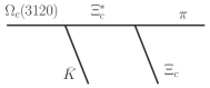
Figure 1: Mechanism for $\Omega_{c}(3120)$ to decay into $\Xi_{c}\bar{K}\pi$ via primary decay into $\Xi_{c}^{*}\bar{K}$.

$$t_{\Omega_{c}\to\pi\bar{K}\Xi_{c}}=g_{\Omega_{c},\bar{K}\Xi^{*}_{c}}\;\dfrac{1}{M_{\rm inv}(\pi\Xi_{c})-M_{\Xi_{c}^{*}}-i\Gamma_{\Xi_{c}^{*}}/2}\;g_{\Xi_{c}^{*},\pi\Xi_{c}}\;\tilde{p}_{\pi},$$ (17)

where

$$\tilde{p}_{\pi}=\dfrac{\lambda^{1/2}(M^{2}_{\rm inv}(\pi\Xi_{c}),m_{\pi}^{2},M^{2}_{\Xi_{c}})}{2\,M_{\rm inv}(\pi\Xi_{c})},$$ (18)

with $g_{\Xi_{c}^{*},\pi\Xi_{c}}$ given using $\Gamma_{\Xi_{c}^{*}}$ as

$$\Gamma_{\Xi_{c}^{*}}=\dfrac{1}{2\,\pi}\;\dfrac{M_{\Xi_{c}}}{M_{\Xi_{c}^{*}}}\;g^{2}_{\Xi_{c}^{*},\pi\Xi_{c}}\,\tilde{p}^{3}_{\pi},$$ (19)

with $\Gamma_{\Xi_{c}^{*}}$ given by Eq. (11).

The mass distribution for the $3$ body decay of the mechanism of Fig. 1 is given by

$$\dfrac{{\rm d}\Gamma_{\Omega_{c}}}{{\rm d}M_{\rm inv}(\pi\Xi_{c})}=\dfrac{1}{(2\pi)^{3}}\;\dfrac{M_{\Xi_{c}}}{M_{\Omega_{c}}}\;p_{\bar{K}}\tilde{p}_{\pi}\;|t_{\Omega_{c}\to\pi\bar{K}\Xi_{c}}|^{2},$$ (20)

with

$$p_{\bar{K}}=\dfrac{\lambda^{1/2}(M_{\Omega_{c}}^{2},m^{2}_{\bar{K}},M^{2}_{\rm inv}(\pi\Xi_{c}))}{2\,M_{\Omega_{c}}},$$ (21)

and the integration over $M_{\rm inv}(\pi\Xi_{c})$ produces the width for $\Omega_{c}(3120)$ decay to $\pi\bar{K}\Xi_{c}$.

The width for $\Omega_{c}(3120)\to\Xi_{c}\bar{K}$ decay can be obtained from

$$\Gamma=\dfrac{1}{2\pi}\;\dfrac{M_{\Xi_{c}}}{M_{\Omega_{c}}}\;g^{2}_{\Omega_{c},\Xi_{c}\bar{K}}\;p^{\prime}_{\bar{K}},$$ (22)

with $p^{\prime}_{\bar{K}}$ the $\bar{K}$ momentum for $\Omega_{c}\to\Xi_{c}\bar{K}$ decay in the $\Omega_{c}$ rest frame.

III Results

We conduct a fit to the position and width of the $\Omega_{c}(3120)$ state using Eq. (5) with the potential of Eq. (2), the $G$ functions of Eqs. (6) and (7) using the second Riemann sheet of Eq. (13). We get a good fit to the data with the parameters

$$\begin{split}q_{\rm max}&=674.6\,\textrm{ MeV},\\ \alpha&=2.6\times 10^{-8}\,\textrm{ MeV}^{-3},\\ \beta&=2.0\times 10^{-9}\,\textrm{ MeV}^{-3}.\end{split}$$ (23)

The pole position appears at

$$(3119.13+i\,0.54)\,\textrm{ MeV}$$ (24)

implying a width of $1.08\textrm{ MeV}$ in agreement with the central values of the experiment.

Now we add the $\Xi_{c}^{*}$ selfenergy in Eq. (II) and look at the $T_{\Xi_{c}^{*}\bar{K}}$ amplitude in the real energy axis. In Fig. 2

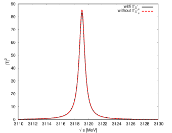
Figure 2: $|T_{\Xi_{c}^{*}\bar{K}}|^{2}$ as a function of $\sqrt{s}$ in the cases with $\Gamma_{\Xi_{c}^{*}}$ and without $\Gamma_{\Xi_{c}^{*}}$, respectively.

we show the results for $|T_{\Xi_{c}^{*}\bar{K}}|^{2}$ with and without the $\Xi_{c}^{*}$ width. As we see, the results are very similar, with the masses and widths practically the same. This means that, unlike in the case of the $\Omega(2012)$, where the difference between the widths in the analogous cases, with $\Xi^{*}$ dressed or without, allowed us to determine the decay width of $\Omega(2012)\to\Xi^{*}\bar{K}\to\Xi\pi\bar{K}$, in the present case we cannot determine the $\Omega_{c}(3120)\to\Xi_{c}^{*}\bar{K}\to\Xi_{c}\pi\bar{K}$ with precision using this procedure. Hence, we use the more accurate one of evaluating the width using explicitly the mechanism of Fig. 1. For this we need the coupling of $\Omega_{c}(3120)\to\Xi_{c}^{*}\bar{K}$, which we address below. The couplings are evaluated at the pole using the $G$ functions in the second Riemann sheet through Eq. (13) and we find the results of Table 1.

Table 1: The couplings $g_{i}$ of $\Omega_{c}(3120)$ to different channels, $g_{i}G_{i}$ and the molecular probabilities for the $S$-wave channels.

	$\Xi_{c}^{*}\bar{K}$	$\Omega^{*}_{c}\eta$	$\Xi_{c}\bar{K}$
$g_{i}$	$2.06-i0.02$	$2.09-i0.01$	$-0.138$
$g_{i}G_{i}$	$-36.77+i0.17$	$-17.64+i0.06$
$-g_{i}^{2}\;\dfrac{\partial G_{i}}{\partial\sqrt{s}}$	$0.63$	$0.10$

We also show there the values of $g_{i}G_{i}$ for the $S$-wave channels, which are the wave functions at the origin in coordinate space Gamermann et al. (2010). As we can see, the wave function is dominated by the $\Xi_{c}^{*}\bar{K}$ component. We ignore now the tiny imaginary part of the couplings and calculate the probability of the $\Xi_{c}^{*}\bar{K},\Omega^{*}_{c}\eta$ channels through $-g_{i}^{2}\;\dfrac{\partial G_{i}}{\partial\sqrt{s}}$ Gamermann et al. (2010); Hyodo (2013). We see again that the $\Xi_{c}^{*}\bar{K}$ has the largest probability of around $63\%$ and the $\Omega_{c}^{*}\eta$ around $10\%$, hence we have a largely molecular state.

Once we have calculated the couplings we are in a position to evaluate the $\Omega_{c}(3120)\to\Xi_{c}^{*}\bar{K}\to\Xi_{c}\pi\bar{K}$ for the mechanism of Fig. 1 through Eqs. (17), (19) and (20). We get

$$\Gamma_{\Omega_{c}\to\Xi_{c}\pi\bar{K}}=0.03\textrm{ MeV},$$ (25)

while through Eq. (22) we would get

$$\Gamma_{\Omega_{c}\to\Xi_{c}\bar{K}}=0.90\textrm{ MeV},$$ (26)

the sum of them giving $\Gamma_{\Omega_{c}}\sim 1\textrm{ MeV}$ as the central value of the experiment, Eq. (8). The fraction of $\Omega_{c}(3120)$ decay to $\Xi_{c}\pi\bar{K}$ is much smaller than the $\Xi\pi\bar{K}$ in the case of the $\Omega(2012)$. However, the molecular probabilities of the $\Xi^{*}_{c}\bar{K}$ and $\Xi^{*}\bar{K}$ in both cases are very similar. The differences stem from the different bindings. In the case of the $\Omega(2012)$ the diagonal terms in the $V$ matrix of Eq. (2) were zero, while here they are finite and negative, indicating extra attraction that reverts into a much bigger binding of about $20\textrm{ MeV}$. This has as a consequence that the decay of the $\Xi_{c}^{*}\bar{K}$ bound component into $\Xi^{*}_{c}\bar{K}\to\Xi_{c}\pi\bar{K}$ is more difficult (technically, the $\Xi_{c}^{*}$ in the diagram of Fig. 1 is more off shell than the $\Xi^{*}$ in the analogous diagram for $\Omega(2012)$ decay). While the experimental determination of a fraction of $0.03\textrm{ MeV}$ is certainly challenging given the present experimental errors in Eq. (8), we look into other experimental tests that can lead us to determine the nature of that state. In Refs. Song et al. (2022); Dai et al. (2023); Song et al. (2023); Li et al. (2023) it was discussed in detail how the knowledge of the binding, scattering length and effective range of the coupled channels provided excellent information on the molecular compositeness of the states. The formalism, improved substantially over the possible application of Weinberg formulas Weinberg (1965), where that range is ignored and leads to unrealistic results in most cases. Anticipating that these magnitudes can be determined, for instance, using correlation functions Tolos and Fabbietti (2020), we determine here the scattering length and effective range of the $\Xi_{c}^{*}\bar{K}$ and $\Omega_{c}^{*}\eta$ channels using the formulas of Ref. Molina et al. (2023),

$$-\dfrac{1}{a_{j}}=\left.-\dfrac{8\pi\,\sqrt{s}}{2\,M_{j}}\;(T_{jj})^{-1}\right|_{\sqrt{s_{{\rm th}}},j},$$ (27)

$$r_{0,j}=\dfrac{1}{\mu_{j}}\;\dfrac{\partial}{\partial\sqrt{s}}\,\left[-\dfrac{8\pi\,\sqrt{s}}{2\,M_{j}}\;(T_{jj})^{-1}+ik_{j}\right]_{\sqrt{s_{{\rm th}}},j},$$ (28)

with $\mu_{j}$ the reduced mass of channel $j$ and $k_{j}$ the momentum of a particle of the pair in their rest frame. The results obtained are shown in Table 2.

Table 2: Scattering length $a_{j}$ and effective range $r_{0,j}$ of the $\Xi_{c}^{*}\bar{K}$ and $\Omega_{c}^{*}\eta$ channels. [in units of fm]

	$a_{j}$	$r_{0,j}$
$\Xi_{c}^{*}\bar{K}$	$1.45-i0.07$	$-0.08-i0.01$
$\Omega^{*}_{c}\eta$	$0.44-i0.09$	$0.26+i0.01$

We can see that the values of $a_{j}$ and $r_{0,j}$ are mostly real, because the main source of decay is to $\Xi_{c}\bar{K}$, which we saw leads to a very small width of the $\Omega_{c}(3120)$ state.

As we can see, we are providing new magnitudes, which are additional to the binding and width of the $\Omega_{c}(3120)$ state. We believe that these magnitudes should be sufficient to determine the nature of the $\Omega_{c}(3120)$ state and the precent work should give an incentive to do experimental work in this direction.

IV Conclusions

We made a thorough study of the $\Omega_{c}(3120)$ state, reported in the LHCb experiment in Ref.  Aaij et al. (2017), which was shown in Ref.  Debastiani et al. (2018) to be well reproduced as a molecular state from the interaction of mostly the $\Xi^{*}_{c}\bar{K}$ and $\Omega_{c}^{*}\eta$ channels. The state has $J^{P}=\frac{3}{2}^{-}$ and is distinct from $\Omega_{c}(3050),\Omega_{c}(3090)(\frac{1}{2}^{-})$ which are generated from the pseudoscalar-baryon $(\frac{1}{2}^{+})$ interaction in Refs.  Montaña et al. (2018); Debastiani et al. (2018). In addition to the $\Xi^{*}_{c}\bar{K},\Omega_{c}^{*}\eta$ channels used in Ref. Debastiani et al. (2018), we include now the $\Xi_{c}\bar{K}$ decay channel, where the state was observed, which appears in $D$-wave. With the consideration of the $\Xi_{c}\bar{K}$ channel, we can now obtain the width of the state, which was not evaluated in Ref.  Debastiani et al. (2018). Then we also evaluate the $\Xi_{c}\pi\bar{K}$ decay width, which could be a measure of the $\Xi^{*}_{c}\bar{K}$ component of the $\Omega_{c}(3120)$ state, but unlike in the analogous $\Omega(2012)$ state where the $\Xi\pi\bar{K}$ decay channel is sizeable and has been measured, providing support for the $\Xi^{*}\bar{K}$ molecular picture of the $\Omega(2012)$ state, here we obtain a very small fraction of $\Xi_{c}\pi\bar{K}$, because the $\Omega_{c}(3120)$ state is more bound than the $\Omega(2012)$. In view of this, we determined the scattering length and effective range of the $\Xi^{*}_{c}\bar{K}$ and $\Omega_{c}^{*}\eta$ channels and made a call for the experimental determination of these magnitudes, accessible for instance measuring correlation functions, which can be instrumental in the determination of the nature of the $\Omega_{c}(3120)$ state.

References

- Yelton et al. (2018) J. Yelton et al. (Belle Collaboration), Phys. Rev. Lett. 121, 052003 (2018), arXiv:1805.09384 [hep-ex] .
- Xiao and Zhong (2018) L.-Y. Xiao and X.-H. Zhong, Phys. Rev. D 98, 034004 (2018), arXiv:1805.11285 [hep-ph] .
- Aliev et al. (2018a) T. M. Aliev, K. Azizi, Y. Sarac, and H. Sundu, Eur. Phys. J. C 78, 894 (2018a), arXiv:1807.02145 [hep-ph] .
- Aliev et al. (2018b) T. M. Aliev, K. Azizi, Y. Sarac, and H. Sundu, Phys. Rev. D 98, 014031 (2018b), arXiv:1806.01626 [hep-ph] .
- Polyakov et al. (2019) M. V. Polyakov, H.-D. Son, B.-D. Sun, and A. Tandogan, Phys. Lett. B 792, 315 (2019), arXiv:1806.04427 [hep-ph] .
- Liu et al. (2020) M.-S. Liu, K.-L. Wang, Q.-F. Lü, and X.-H. Zhong, Phys. Rev. D 101, 016002 (2020), arXiv:1910.10322 [hep-ph] .
- Arifi et al. (2022) A. J. Arifi, D. Suenaga, A. Hosaka, and Y. Oh, Phys. Rev. D 105, 094006 (2022), arXiv:2201.10427 [hep-ph] .
- Wang et al. (2023) K.-L. Wang, Q.-F. Lü, J.-J. Xie, and X.-H. Zhong, Phys. Rev. D 107, 034015 (2023), arXiv:2203.04458 [hep-ph] .
- Valderrama (2018) M. P. Valderrama, Phys. Rev. D 98, 054009 (2018), arXiv:1807.00718 [hep-ph] .
- Lin and Zou (2018) Y.-H. Lin and B.-S. Zou, Phys. Rev. D 98, 056013 (2018), arXiv:1807.00997 [hep-ph] .
- Pavao and Oset (2018) R. Pavao and E. Oset, Eur. Phys. J. C 78, 857 (2018), arXiv:1808.01950 [hep-ph] .
- Huang et al. (2018a) Y. Huang, M.-Z. Liu, J.-X. Lu, J.-J. Xie, and L.-S. Geng, Phys. Rev. D 98, 076012 (2018a), arXiv:1807.06485 [hep-ph] .
- Lu et al. (2020) J.-X. Lu, C.-H. Zeng, E. Wang, J.-J. Xie, and L.-S. Geng, Eur. Phys. J. C 80, 361 (2020), arXiv:2003.07588 [hep-ph] .
- Ikeno et al. (2020) N. Ikeno, G. Toledo, and E. Oset, Phys. Rev. D 101, 094016 (2020), arXiv:2003.07580 [hep-ph] .
- Liu et al. (2021) X. Liu, H. Huang, J. Ping, and D. Chen, Phys. Rev. C 103, 025202 (2021), arXiv:2010.15398 [hep-ph] .
- Hofmann and Lutz (2006) J. Hofmann and M. F. M. Lutz, Nucl. Phys. A 776, 17 (2006), arXiv:hep-ph/0601249 .
- Sarkar et al. (2005) S. Sarkar, E. Oset, and M. J. Vicente Vacas, Nucl. Phys. A 750, 294 (2005), [Erratum: Nucl.Phys.A 780, 90–90 (2006)], arXiv:nucl-th/0407025 .
- Wang et al. (2007) W.-L. Wang, F. Huang, Z.-Y. Zhang, Y.-W. Yu, and F. Liu, Commun. Theor. Phys. 48, 695 (2007).
- Wang et al. (2008) W. L. Wang, F. Huang, Z. Y. Zhang, and F. Liu, J. Phys. G 35, 085003 (2008).
- Gutsche and Lyubovitskij (2020) T. Gutsche and V. E. Lyubovitskij, J. Phys. G 48, 025001 (2020), arXiv:1912.10894 [hep-ph] .
- Jia et al. (2019) S. Jia et al. (Belle Collaboration), Phys. Rev. D 100, 032006 (2019), arXiv:1906.00194 [hep-ex] .
- Belle (2022) Belle (Belle Collaboration), (2022), arXiv:2207.03090 [hep-ex] .
- Aaij et al. (2017) R. Aaij et al. (LHCb Collaboration), Phys. Rev. Lett. 118, 182001 (2017), arXiv:1703.04639 [hep-ex] .
- Aaij et al. (2023) R. Aaij et al. (LHCb Collaboration), Phys. Rev. Lett. 131, 131902 (2023), arXiv:2302.04733 [hep-ex] .
- Ebert et al. (2008) D. Ebert, R. N. Faustov, and V. O. Galkin, Phys. Lett. B 659, 612 (2008), arXiv:0705.2957 [hep-ph] .
- Roberts and Pervin (2008) W. Roberts and M. Pervin, Int. J. Mod. Phys. A 23, 2817 (2008), arXiv:0711.2492 [nucl-th] .
- Garcilazo et al. (2007) H. Garcilazo, J. Vijande, and A. Valcarce, J. Phys. G 34, 961 (2007), arXiv:hep-ph/0703257 .
- Migura et al. (2006) S. Migura, D. Merten, B. Metsch, and H.-R. Petry, Eur. Phys. J. A 28, 41 (2006), arXiv:hep-ph/0602153 .
- Ebert et al. (2011) D. Ebert, R. N. Faustov, and V. O. Galkin, Phys. Rev. D 84, 014025 (2011), arXiv:1105.0583 [hep-ph] .
- Valcarce et al. (2008) A. Valcarce, H. Garcilazo, and J. Vijande, Eur. Phys. J. A 37, 217 (2008), arXiv:0807.2973 [hep-ph] .
- Shah et al. (2016) Z. Shah, K. Thakkar, A. K. Rai, and P. C. Vinodkumar, Chin. Phys. C 40, 123102 (2016), arXiv:1609.08464 [nucl-th] .
- Vijande et al. (2013) J. Vijande, A. Valcarce, T. F. Carames, and H. Garcilazo, Int. J. Mod. Phys. E 22, 1330011 (2013), arXiv:1212.4383 [hep-ph] .
- Yoshida et al. (2015) T. Yoshida, E. Hiyama, A. Hosaka, M. Oka, and K. Sadato, Phys. Rev. D 92, 114029 (2015), arXiv:1510.01067 [hep-ph] .
- Chen et al. (2015) H.-X. Chen, W. Chen, Q. Mao, A. Hosaka, X. Liu, and S.-L. Zhu, Phys. Rev. D 91, 054034 (2015), arXiv:1502.01103 [hep-ph] .
- Chen et al. (2016) H.-X. Chen, Q. Mao, A. Hosaka, X. Liu, and S.-L. Zhu, Phys. Rev. D 94, 114016 (2016), arXiv:1611.02677 [hep-ph] .
- Chiladze and Falk (1997) G. Chiladze and A. F. Falk, Phys. Rev. D 56, R6738 (1997), arXiv:hep-ph/9707507 .
- Manohar and Georgi (1984) A. Manohar and H. Georgi, Nucl. Phys. B 234, 189 (1984).
- Agaev et al. (2017a) S. S. Agaev, K. Azizi, and H. Sundu, Eur. Phys. J. C 77, 395 (2017a), arXiv:1704.04928 [hep-ph] .
- Agaev et al. (2017b) S. S. Agaev, K. Azizi, and H. Sundu, EPL 118, 61001 (2017b), arXiv:1703.07091 [hep-ph] .
- Wang (2017) Z.-G. Wang, Eur. Phys. J. C 77, 325 (2017), arXiv:1704.01854 [hep-ph] .
- Hofmann and Lutz (2005) J. Hofmann and M. F. M. Lutz, Nucl. Phys. A 763, 90 (2005), arXiv:hep-ph/0507071 .
- Jimenez-Tejero et al. (2009) C. E. Jimenez-Tejero, A. Ramos, and I. Vidana, Phys. Rev. C 80, 055206 (2009), arXiv:0907.5316 [hep-ph] .
- Romanets et al. (2012) O. Romanets, L. Tolos, C. Garcia-Recio, J. Nieves, L. L. Salcedo, and R. G. E. Timmermans, Phys. Rev. D 85, 114032 (2012), arXiv:1202.2239 [hep-ph] .
- Xin et al. (2023) Q. Xin, X.-S. Yang, and Z.-G. Wang, Int. J. Mod. Phys. A 38, 2350123 (2023), arXiv:2307.08926 [hep-ph] .
- Karliner and Rosner (2017) M. Karliner and J. L. Rosner, Phys. Rev. D 95, 114012 (2017), arXiv:1703.07774 [hep-ph] .
- Wang et al. (2017) K.-L. Wang, L.-Y. Xiao, X.-H. Zhong, and Q. Zhao, Phys. Rev. D 95, 116010 (2017), arXiv:1703.09130 [hep-ph] .
- Wang and Zhu (2017) W. Wang and R.-L. Zhu, Phys. Rev. D 96, 014024 (2017), arXiv:1704.00179 [hep-ph] .
- Chen and Liu (2017) B. Chen and X. Liu, Phys. Rev. D 96, 094015 (2017), arXiv:1704.02583 [hep-ph] .
- Yang and Ping (2018) G. Yang and J. Ping, Phys. Rev. D 97, 034023 (2018), arXiv:1703.08845 [hep-ph] .
- Huang et al. (2018b) H. Huang, J. Ping, and F. Wang, Phys. Rev. D 97, 034027 (2018b), arXiv:1704.01421 [hep-ph] .
- Kim et al. (2017) H.-C. Kim, M. V. Polyakov, and M. Praszałowicz, Phys. Rev. D 96, 014009 (2017), [Addendum: Phys.Rev.D 96, 039902 (2017)], arXiv:1704.04082 [hep-ph] .
- An and Chen (2017) C. S. An and H. Chen, Phys. Rev. D 96, 034012 (2017), arXiv:1705.08571 [hep-ph] .
- Ali et al. (2017) A. Ali, J. S. Lange, and S. Stone, Prog. Part. Nucl. Phys. 97, 123 (2017), arXiv:1706.00610 [hep-ph] .
- Anisovich et al. (2017) V. V. Anisovich, M. A. Matveev, J. Nyiri, and A. N. Semenova, Mod. Phys. Lett. A 32, 1750154 (2017), arXiv:1706.01336 [hep-ph] .
- Padmanath and Mathur (2017) M. Padmanath and N. Mathur, Phys. Rev. Lett. 119, 042001 (2017), arXiv:1704.00259 [hep-ph] .
- Montaña et al. (2018) G. Montaña, A. Feijoo, and A. Ramos, Eur. Phys. J. A 54, 64 (2018), arXiv:1709.08737 [hep-ph] .
- Debastiani et al. (2018) V. R. Debastiani, J. M. Dias, W. H. Liang, and E. Oset, Phys. Rev. D 97, 094035 (2018), arXiv:1710.04231 [hep-ph] .
- Bando et al. (1985) M. Bando, T. Kugo, S. Uehara, K. Yamawaki, and T. Yanagida, Phys. Rev. Lett. 54, 1215 (1985).
- Bando et al. (1988) M. Bando, T. Kugo, and K. Yamawaki, Phys. Rept. 164, 217 (1988).
- Meissner (1988) U. G. Meissner, Phys. Rept. 161, 213 (1988).
- Nagahiro et al. (2009) H. Nagahiro, L. Roca, A. Hosaka, and E. Oset, Phys. Rev. D 79, 014015 (2009), arXiv:0809.0943 [hep-ph] .
- Capstick and Isgur (1986) S. Capstick and N. Isgur, Phys. Rev. D 34, 2809 (1986).
- Song et al. (2022) J. Song, L. R. Dai, and E. Oset, Eur. Phys. J. A 58, 133 (2022), arXiv:2201.04414 [hep-ph] .
- Dai et al. (2023) L. R. Dai, J. Song, and E. Oset, Phys. Lett. B 846, 138200 (2023), arXiv:2306.01607 [hep-ph] .
- Song et al. (2023) J. Song, L. R. Dai, and E. Oset, (2023), arXiv:2307.02382 [hep-ph] .
- Li et al. (2023) H.-P. Li, J. Song, W.-H. Liang, R. Molina, and E. Oset, (2023), arXiv:2311.14365 [hep-ph] .
- Dai et al. (2022) L. R. Dai, E. Oset, A. Feijoo, R. Molina, L. Roca, A. M. Torres, and K. P. Khemchandani, Phys. Rev. D 105, 074017 (2022), [Erratum: Phys.Rev.D 106, 099904 (2022)], arXiv:2201.04840 [hep-ph] .
- Gamermann et al. (2010) D. Gamermann, J. Nieves, E. Oset, and E. Ruiz Arriola, Phys. Rev. D 81, 014029 (2010), arXiv:0911.4407 [hep-ph] .
- Hyodo (2013) T. Hyodo, Int. J. Mod. Phys. A 28, 1330045 (2013), arXiv:1310.1176 [hep-ph] .
- Weinberg (1965) S. Weinberg, Phys. Rev. 137, B672 (1965).
- Tolos and Fabbietti (2020) L. Tolos and L. Fabbietti, Prog. Part. Nucl. Phys. 112, 103770 (2020), arXiv:2002.09223 [nucl-ex] .
- Molina et al. (2023) R. Molina, C.-W. Xiao, W.-H. Liang, and E. Oset, (2023), arXiv:2310.12593 [hep-ph] .