Ultracold coherent control of molecular collisions at a Förster resonance

Abstract

We show that the precise preparation of a quantum superposition between three rotational states of an ultracold dipolar molecule generates controllable interferences in their two-body scattering dynamics and collisional rate coefficients, at an electric field that produces a Förster resonance. This proposal represents a feasible protocol to achieve coherent control on ultracold molecular collisions in current experiments. It sets the basis for future studies in which one can think to control the amount of each produced pairs, including trapped entangled pairs of reactants, individual pairs of products in a chemical reaction, and measuring each of their scattering phase-shifts that could envision “complete chemical experiments” at ultracold temperatures.

The advent of ultracold, controlled dipolar molecules has opened many exciting perspectives for the field of ultracold matter. Their extremely controllable properties have inspired many theoretical proposals for promising quantum applications, such as quantum simulation and quantum information processes, quantum-controlled chemistry and test of fundamental laws Bohn et al. (2017); DeMille et al. (2017). The molecules can be well prepared in individual quantum states Ni et al. (2008), their long-range interactions can be controlled Quéméner and Julienne (2012), they can be long-lived and protected from their environment Micheli et al. (2010); Quéméner and Bohn (2010); de Miranda et al. (2011); Chotia et al. (2012); Frisch et al. (2015); Wang and Quéméner (2015); Karman and Hutson (2018); Lassablière and Quéméner (2018); Xie et al. (2020); Karam et al. (2023); Matsuda et al. (2020); Li et al. (2021); Anderegg et al. (2021); Schindewolf et al. (2022); Bigagli et al. (2023a); Lin et al. (2023), enabling the formation of quantum degenerate gases De Marco et al. (2019); Valtolina et al. (2020); Schindewolf et al. (2022); Bigagli et al. (2023b), they can be manipulated in optical lattices Yan et al. (2013); Christakis et al. (2023) or in optical tweezers Liu et al. (2018); Anderegg et al. (2019); Ruttley et al. (2023), they can be used to explore many-body effects Micheli et al. (2006); Büchler et al. (2007); Gorshkov et al. (2011); Baranov et al. (2012); Yao et al. (2018); Schmidt et al. (2022), they can be electro-associated to form long-range tetramer molecules Quéméner et al. (2023); Chen et al. (2023), and they can be entangled Holland et al. (2022); Bao et al. (2022). Ultracold molecules can also be used to probe chemical reactions with an unprecedented control at the quantum level, as was done with the chemical reaction KRb + KRb $\to$ K₂ + Rb₂ at ultracold temperatures Hu et al. (2019); Liu et al. (2021), including the control of the rotational parity of the products Hu et al. (2021); Quéméner et al. (2021) and the creation of entangled product pairs Liu et al. (2023).

In this study, we propose to apply the ideas of coherent control Shapiro and Brumer (1996); Brumer et al. (2000); Shapiro and Brumer (2003); Gong et al. (2003); Devolder et al. (2021, 2022, 2023a, 2023b) to current experiments of ultracold chemical reactions Matsuda et al. (2020); Li et al. (2021); Liu et al. (2021). By using a microwave to prepare ultracold dipolar molecules in a quantum superposition of three stationary states (qutrit) and by using a static electric field to make collisional states degenerate, we predict that one can observe interferences in the rate coefficients of ultracold molecules. This work provides a realistic and concrete experimental set-up for current experiments to observe interferences and coherent control in ultracold collisions.

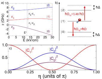
Figure 1: a) Energies $\varepsilon_{0}$, $\varepsilon_{1}$, $\varepsilon_{2}$ of the dressed states $\ket{0}$, $\ket{1}$, $\ket{2}$ as a function of the electric field $E$ (with all $m_{j}=0$). b) Sketch of the same energies at the Förster resonance located at $E=E^{*}=12.506$ kV/cm representing a ladder configuration in the presence of a microwave. As the levels are equally spaced, the microwave creates a coupling between $\ket{0}$, $\ket{1}$ and $\ket{1}$, $\ket{2}$, with a detuning $\hbar\Delta$ and Rabi frequencies $\Omega_{01}\equiv\Omega$ and $\Omega_{12}\equiv\chi\,\Omega\approx 1.48\,\Omega$. c) Evolution of the coefficient $|C_{0,1,2}|^{2}$ as a function of $\eta$ when $\Delta=0$.

We first consider an ultracold dipolar gas of fermionic ${}^{40}\text{K}^{87}\text{Rb}$ molecules, taken as an example, in their ground electronic and vibrational state, and in their first excited rotational state. Their rotational states will be denoted by the kets $\ket{j,m_{j}}$, using usual notations for their quantum numbers $j$ and $m_{j}$. We omit the hyperfine structure and the nuclear spins of the atoms as they remain spectators at the magnetic fields considered in current experiments Matsuda et al. (2020); Li et al. (2021). In a static dc electric field $E$, the molecules are dressed into new states $\ket{\tilde{j},m_{j}}$ (also noted $\ket{j}$ for simplicity), preserving the value of $m_{j}$. These are stationary states with well defined energies $\varepsilon_{j}$, as illustrated in Fig. 1a as a function of $E$. Following the experiments in Matsuda et al. (2020); Li et al. (2021), we assume that all the molecules are prepared in a dressed state $\ket{\tilde{1},0}$, noted $\ket{1}$, with energy $\varepsilon_{1}$ and we will assume a collision energy of $E_{c}/k_{B}=500$ nK. Two other states, namely $\ket{\tilde{0},0}$ (noted $\ket{0}$) with energy $\varepsilon_{0}$ and $\ket{\tilde{2},0}$ (noted $\ket{2}$) with energy $\varepsilon_{2}$, will be of interest in the following. We impose the electric field to be $E=E^{*}=12.506$ kV/cm, reachable in those experiments and for which $\varepsilon_{1}-\varepsilon_{0}$ = $\varepsilon_{2}-\varepsilon_{1}$. This characterizes the position of a Förster resonance Comparat and Pillet (2010).

Then, by applying a linearly polarized microwave of defined frequency and intensity during a time $\tau$, we couple the states $\ket{0}$ and $\ket{2}$ to the state $\ket{1}$, and create Rabi oscillations between those three stationary states, consequently forming a qutrit. This is illustrated in Fig. 1b. The frequency of the microwave defines an equal detuning $\hbar\Delta$ as the energy spacings are the same, while its intensity defines an ac electric field $E_{ac}$, corresponding to two Rabi frequencies $\Omega_{10}=\tilde{d}^{1\leftrightarrow 0}\,E_{ac}/\hbar\equiv\Omega$ and $\Omega_{12}=\tilde{d}^{1\leftrightarrow 2}\,E_{ac}/\hbar\equiv\chi\,\Omega$, depending on the electric dipole moments of the transitions. The quantities $\tilde{d}^{1\leftrightarrow 2}=0.293$ D and $\tilde{d}^{1\leftrightarrow 0}=0.198$ D are generalized induced dipole moments at $E^{*}$ Lassablière and Quéméner (2022), the ratio of which gives $\chi\approx 1.48$. This prepares a quantum superposition defined by the wavefunction at any time $t\geq\tau$

$$\ket{\Psi_{mol}}=\sum_{i=0}^{2}{c}_{i}\ket{i}e^{\text{i}(\vec{k}_{i}.\vec{\rho}-\omega_{i}t)}\equiv\sum_{i=0}^{2}C_{i}\ket{i}e^{\text{i}(\vec{k}_{i}.\vec{\rho}-\omega_{i}(t-\tau))}$$

with ${c}_{i}=C_{i}\,e^{\text{i}\omega_{i}\tau}$, $\vec{k}_{i}$ and $\hbar\omega_{i}=\hbar^{2}k_{i}^{2}/2m+\varepsilon_{i}$ are respectively the initial wavevector and energy of the individual molecule of mass $m$, described by a position vector $\vec{\rho}$, formed in states $i$. Due to negligible recoil energy and Doppler effect for a microwave transition SM , the wavevector of the molecule when excited in state $\ket{2}$ or de-excited in state $\ket{0}$ is the same as the initial one in state $\ket{1}$, namely $\vec{k}_{2}\simeq\vec{k}_{0}\simeq\vec{k}_{1}$.

Control of the interferences is reached through the control of this quantum superposition and the $C_{i}$ factors. This is achieved by monitoring the parameters $\Delta$, $\Omega$ and $\tau$. At the Förster resonance, the dynamics of the superposition is dictated by the resulting light-matter Hamiltonian. To keep this work general, we will focus on the condition $\Delta=0$ for which the superposition factors are analytical. At time $t=\tau$, the microwave is turned off and the $C_{i}$ factors are well defined SM given by $C_{1}=\cos\eta$, $C_{0}=-\text{i}\sin\Theta\sin\eta$, $C_{2}=-\text{i}\cos\Theta\sin\eta$, with $\eta=\sqrt{1+\chi^{2}}\,\Omega\,\tau/2$ and $\tan\Theta=\Omega_{10}/\Omega_{12}=1/\chi\approx 0.68$. The modulus square of these factors are represented in Fig. 1c. The preparation time $\tau$ should be shorter than a typical collisional time ($\tau\ll\tau_{col}\simeq 1$ ms for KRb molecules at $E^{*}$).

Then after a time $t\geq\tau$, the molecules are free to collide. The overall incident collisional wavefunction between two molecules Brumer et al. (2000); Shapiro and Brumer (2003) prepared as in Eq. (Ultracold coherent control of molecular collisions at a Förster resonance) is

$$\ket{\Psi_{col}^{inc}}=\ket{\Psi_{mol}}\otimes\ket{\Psi_{mol}}\\ =\sum_{\alpha}^{*}C_{\alpha}\ket{\alpha}e^{\text{i}\vec{k}_{{\alpha}}.\vec{r}}e^{\text{i}\vec{K}_{\alpha}.\vec{R}}e^{-\text{i}\omega_{\alpha}(t-\tau)}$$ (2)

where $\vec{k}_{{\alpha}}$, $\vec{K}_{{\alpha}}$ and $\hbar\omega_{\alpha}=\hbar^{2}k_{\alpha}^{2}/2\mu+\hbar^{2}K_{\alpha}^{2}/2M+\varepsilon_{\alpha}$ are respectively the initial wavevector of the relative motion of reduced mass $\mu=m/2$ described by a position vector $\vec{r}$, the initial wavevector of the center-of-mass motion of total mass $M=2m$ described by a position vector $\vec{R}$, and the energy of the two molecules initialy prepared in one of the six possible combined molecular states $\ket{\alpha}\equiv\ket{00},\ket{11},\ket{22},\ket{01+},\ket{12+},\ket{02+}$, arising from the possible combinations of states $\ket{0},\ket{1},\ket{2}$ in Eq. (Ultracold coherent control of molecular collisions at a Förster resonance). The internal energy $\varepsilon_{\alpha}$ of these states are plotted in Fig 2a as a function of $E$. These combined molecular states are properly symmetrized under exchange of identical particles SM . The asterisk sign over the sum in Eq. (2) means that the states $\alpha$ are retricted to the six ones mentioned above. The $C_{\alpha}$ factors are given by $C_{11}=\cos^{2}\eta$, $C_{00}=-\sin^{2}\Theta\sin^{2}\eta$, $C_{22}=-\cos^{2}\Theta\sin^{2}\eta$, $C_{01+}=-\text{i}\sqrt{2}\sin\Theta\sin\eta\cos\eta$, $C_{12+}=-\text{i}\sqrt{2}\cos\Theta\sin\eta\cos\eta$, $C_{02+}=-\sqrt{2}\sin\Theta\cos\Theta\sin^{2}\eta$ SM , the modulus square of which are represented in Fig 2c.

Eq. (2) is then a quantum superposition of six possible incident wavefunctions. Each of them have a well defined energy $\hbar\omega_{\alpha}$ and produces a scattered wavefunction that we can compute Wang and Quéméner (2015) as the result of the collision. Note that the goal of the microwave preparation is not to keep the coherence of the individual molecules, as these scattered terms will definitively destroy the qutrits, but rather to populate different molecular collisional states with the controlled $C_{\alpha}$ factors. The asymptotic form of the general wavefunction of the system is then given by the quantum superposition of different collisional wavefunctions

$$\ket{\Psi_{col}}\underset{r\to\infty}{=}\sum_{\alpha}^{*}\,\bigg{[}C_{\alpha}\,\ket{\alpha}\,e^{\text{i}\vec{k}_{{\alpha}}.\vec{r}}\\ +{\sum_{\alpha^{\prime}}}C_{\alpha}\,f^{scat}_{{\alpha\to\alpha^{\prime}}}(\vec{k}_{\alpha},\hat{r})\,\frac{e^{\text{i}k^{\alpha}_{\alpha^{\prime}}r}}{r}\ket{\alpha^{\prime}}\bigg{]}e^{\text{i}\vec{K}_{\alpha}.\vec{R}}\,e^{-\text{i}\omega_{\alpha}(t-\tau)}$$ (3)

with the scattering amplitude given by

$$f^{scat}_{\alpha\to\alpha^{\prime}}(\vec{k}_{\alpha},\hat{r})=\frac{2\pi}{\text{i}\,k_{\alpha}^{1/2}\,{k^{\alpha}_{\alpha^{\prime}}}^{1/2}}\,\sum_{l=0}^{\infty}\sum_{m_{l}=-l}^{l}\sum_{l^{\prime}=0}^{\infty}\sum_{m_{l}^{\prime}=-l^{\prime}}^{l^{\prime}}\\ \text{i}^{l-l^{\prime}}\,[Y_{l}^{m_{l}}(\hat{k}_{\alpha})]^{*}\,Y_{l^{\prime}}^{m_{l}^{\prime}}(\hat{r})\,T_{\alpha^{\prime}\,l^{\prime}\,m_{l}^{\prime},\alpha\,l\,m_{l}}(k_{\alpha})$$ (4)

in term of elements of the transition matrix $T$ that we can compute, employing an usual partial wave expansion over $l,m_{l},l^{\prime},m_{l}^{\prime}$, for a given total angular momentum projection quantum number $M$ Wang and Quéméner (2015). The quantities $k^{\alpha}_{\alpha^{\prime}}$ are found using the conservation of energy after a collision $\hbar^{2}\,({k^{\alpha}_{\alpha^{\prime}}})^{2}/2\mu+\varepsilon_{\alpha^{\prime}}$ = $E_{c}+\varepsilon_{\alpha}$. Note that the states $\alpha^{\prime}$ are all the possible combined molecular states to which the system can end up after a collision and are not restricted to the six ones prepared in Eq. (2). For example, molecules can end up in states with values of $m_{j}\neq 0$ such as $\ket{\tilde{1},\pm 1}$, $\ket{\tilde{2},\pm 1}$, $\ket{\tilde{2},\pm 2}$ and this is included in our study Wang and Quéméner (2015).

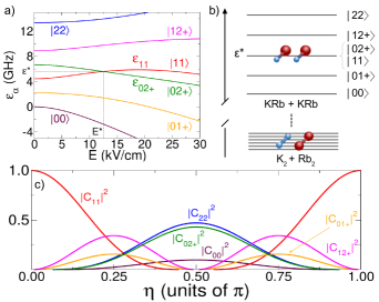
Figure 2: a) Energies $\varepsilon_{\alpha}$ with $\alpha=00,01+,11,02+,12+,22$ as a function of $E$ (with all $m_{j}=0$). At $E^{*}$, the energy $\varepsilon_{11}=\varepsilon_{02+}\equiv\varepsilon^{*}$. Not shown, energies for combined molecular states including non-zero values of $m_{j}$. b) Sketch of the same energies at the Förster resonance. c) Evolution of the coefficient $|C_{\alpha}|^{2}$ as a function of $\eta$ when $\Delta=0$.

Because $\vec{k}_{2}\simeq\vec{k}_{0}\simeq\vec{k}_{1}$ as mentioned earlier in Eq. (Ultracold coherent control of molecular collisions at a Förster resonance), all the vectors $\vec{k}_{{\alpha}}$ are also equal SM (we will note them $\vec{k}$) and the related collision energies $\hbar^{2}k_{\alpha}^{2}/2\mu$ are the same as the initial molecules in the gas, namely $E_{c}/k_{B}=500$ nK. Similarly, all the vectors $\vec{K}_{{\alpha}}$ are equal (we will note them $\vec{K}$) so that the six possible centers-of-mass, where a collision can take place, move in the same way. This is in fact a minimal requirement needed to expect for interferences between the six collisional waves in Eq. (3). However, if the angular frequencies $\omega_{\alpha}$ appearing in the time-dependent terms are different, the six collisional waves are not synchronous, that is they will not occur at the same time. They will do so if and only if the combined molecular states $\ket{\alpha}$ have the same internal energies $\varepsilon_{\alpha}$ Brumer et al. (2000); Shapiro and Brumer (2003). This is in general not an obvious requirement to fulfill. But this can be done precisely for the states $\ket{11}$ and $\ket{02+}$ at $E=E^{*}$, by definition of the Förster resonance, where $\varepsilon_{11}=\varepsilon_{02+}=\varepsilon^{*}$, as illustrated in Fig. 2b. Then $\hbar\omega_{11}=\hbar\omega_{02+}$ (we note them $\hbar\omega$) and $k^{11}_{\alpha^{\prime}}=k^{02+}_{\alpha^{\prime}}$ (we note them $k^{11/02+}_{\alpha^{\prime}}$). As the states $\ket{11}$ and $\ket{02+}$ collide in the same center-of-mass and become synchronous, they can interfere. This is the key point of the paper. We can factorize those two terms in Eq. (3) to get the interference part of the collisional wavefunction

$$\ket{\Psi_{col}^{int}}\underset{r\to\infty}{=}\bigg{\{}\bigg{[}C_{11}\,\ket{11}+C_{02+}\,\ket{02+}\bigg{]}\,e^{\text{i}\vec{k}.\vec{r}}\\ +\sum_{\alpha^{\prime}}\bigg{[}C_{11}\,f^{scat}_{11\to\alpha^{\prime}}+C_{02+}\,f^{scat}_{02+\to\alpha^{\prime}}\bigg{]}\,\ket{\alpha^{\prime}}\,\frac{e^{\text{i}k^{11/02+}_{\alpha^{\prime}}r}}{r}\bigg{\}}\\ e^{\text{i}\vec{K}.\vec{R}}\,e^{-\text{i}\omega(t-\tau)}.$$ (5)

For the four remaining terms $\alpha=00,22,01+,12+$, also called “satellite” terms Brumer et al. (2000); Shapiro and Brumer (2003); Gong et al. (2003), they do not interfere in Eq. (3) and will provide each of them an independent result. For a starting quantum superposition state, one can then define in Eq. (5) new expressions of Brumer et al. (2000); Shapiro and Brumer (2003); Gong et al. (2003); Devolder et al. (2021)

$$f^{qs}_{11/02+\,\rightarrow\alpha^{\prime}} = C_{11}f^{scat}_{11\rightarrow\alpha^{\prime}}+C_{02+}f^{scat}_{02+\rightarrow\alpha^{\prime}}$$ (6)

$$T^{qs}_{\alpha^{\prime}l^{\prime}m_{l}^{\prime},11/02+\,lm_{l}} = C_{11}T_{\alpha^{\prime}l^{\prime}m_{l}^{\prime},11\,lml}+C_{02+}T_{\alpha^{\prime}l^{\prime}m_{l}^{\prime},02+\,lm_{l}}$$

where the notation $11/02+$ is used now to illustrate that $11$ and $02+$ are interfering and cannot be considered separately, and

$$f^{qs}_{\alpha\rightarrow\alpha^{\prime}} =C_{\alpha}f^{scat}_{\alpha\rightarrow\alpha^{\prime}} T^{qs}_{\alpha^{\prime}l^{\prime}m_{l}^{\prime},\alpha lm_{l}} =C_{\alpha}T_{\alpha^{\prime}l^{\prime}m_{l}^{\prime},\alpha lml}$$ (7)

for the satellite terms. The rate coefficient ending in any combined molecular state $\alpha^{\prime}$ is given by

$$\beta^{qs}_{\alpha^{\prime}}(E_{c})=\sum_{\alpha}^{*}\beta^{qs}_{\alpha\rightarrow\alpha^{\prime}}(E_{c})$$ (8)

where the sum runs over $\alpha=11/02+$, $00$, $01+$, $12+$, $22$, with

$$\beta^{qs}_{\alpha\rightarrow\alpha^{\prime}}(E_{c})=2\,\frac{\pi\hbar}{\mu k}\sum_{l}\sum_{m_{l}}\sum_{l^{\prime}}\sum_{m_{l}^{\prime}}\left|T^{qs}_{\alpha^{\prime}l^{\prime}m_{l}^{\prime},\alpha lm_{l}}\right|^{2}.$$ (9)

The rate coefficients depend parametrically on $\eta$ via the $C_{\alpha}$ coefficients in Eq. (6) and Eq. (7). The factor of 2 takes into account that the initial molecules are indistinguishable. The overall reactive rate coefficient is given by SM

$$\beta^{qs}_{re}(E_{c})=\sum_{\alpha}^{*}2\,\frac{\hbar\pi}{\mu k}\,|C_{\alpha}|^{2}\,\sum_{l}\sum_{m_{l}}P^{re}_{\alpha lm_{l}}$$ (10)

where the sum runs over $\alpha=$ $11$, $02+$, $00$, $01+$, $12+$, $22$.

We computed all the $T$ and $P^{re}$ elements apearing in Eq. (9) and Eq. (10) at $E_{c}/k_{B}=500$ nK, using the same basis sets as in Wang and Quéméner (2015) that showed very good agreement with experimental observations in a free-space 3D geometry ($M=0,\pm 1$, $l=1,3,5$, see conditions in Li et al. (2021)) and in a confined quasi-2D geometry ($M=\pm 1$, $l=1,3,5$, see conditions in Matsuda et al. (2020)). We plot the corresponding rate coefficients in Fig. (3) for the free-space case and in Fig. (4) for the confined case. In all cases, the rate to a state $\alpha^{\prime}$ in Eq. (8) comes mainly from the contribution of the elastic term $\alpha=\alpha^{\prime}$ in Eq. (9), those for which the kinetic energy of the relative motion of the two molecules does not change Hutson (2009). It means that all the final reactants in a state $\alpha^{\prime}$ have mainly the same final kinetic energies than their initial ones, so that they remain ultracold and still trapped.

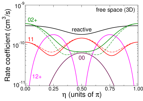
Figure 3: Rate coefficients $\beta^{qs}_{\alpha^{\prime}}$ of two qutrits at a Förster resonnance as a function of the control parameter $\eta$, in a free-space 3D geometry at $E_{c}/k_{B}=500$ nK. The solid red (resp. green) curve corresponds to a measurement in the final state $\alpha^{\prime}=11$ (resp. $\alpha^{\prime}=02+$). The dashed curves corresponds to the same curves but if there were no interferences. The solid black curve corresponds to the overall reactive rate coefficient. The solid brown (resp. pink) curve corresponds to a measurement in the final state $\alpha^{\prime}=00$ (resp. $\alpha^{\prime}=12+$).

First, we can see on both figures that the rates present variations as a function of $\eta$. Though, for $\alpha^{\prime}=00$ (solid brown curves) and $12+$ (solid pink curves), they do not correspond to interferences as can be seen from Eq. (7). The rates are just respectively proportional to $|C_{00}|^{2}$ and $|C_{12+}|^{2}$ in Eq. (9). They just exhibit the same $\eta$ behaviour as those preparation coefficients, as can be seen in Fig. 2c. The rates to $\alpha^{\prime}=01+$, $22+$, as well as to the other combined molecular states involving $m_{j}\neq 0$ are much smaller and do not appear in the figure. For $\alpha^{\prime}=11$ (solid red curves) and $02+$ (solid green curves) for the free-space case, the variations correspond to destructive and constructive interferences respectively, when compared to the same rates (dashed curves) without the crossed interference term taken into account in Eq. (8) and Eq. (6). By controlling individually $C_{11}$ and $C_{02+}$ with $\eta$, one coherently controls the scattering amplitude and the $T$ matrix elements, hence the observables $\beta^{qs}_{11}$ and $\beta^{qs}_{02+}$, with changes of magnitude up to a factor of five here. For the confined case, similar conclusions hold but now both states $\alpha^{\prime}=11$ and $02+$ correspond to constructive interferences.

Secondly, the rich physics at this Förster resonance is a remarkable source for ultracold entangled pairs remaining in the trap. As can be seen for $\eta=0$ (conditions already fulfilled in Matsuda et al. (2020); Li et al. (2021)), we predict a large production in $\alpha^{\prime}=02+$, namely trapped pairs in the entangled states $\ket{02+}=\{\ket{02}+\ket{20}\}/\sqrt{2}$, even larger than the production in the non-entangled trapped pairs $\alpha^{\prime}=11$, or in the non-trapped reactive pairs. When $\eta$ increases from 0 to $\pi/2$, it turns out that $\beta^{qs}_{02+}$ decreases in a monotonic way. Even though interferences are constructive, the fact that the coefficients $C_{11}$ and $C_{02+}$ are purely real numbers for $\Delta=0$ (without additional phases to monitor), decreases somewhat the flexibility to control the amount of interferences in Eq. (6). However, if we consider the case $\Delta\neq 0$, the $C_{11}$ and $C_{02+}$ coefficients become arbitrary complex numbers (including two phases to monitor) that can be controlled in many ways by the three independent values $\Delta$, $\Omega$, and $\tau$. This can be used to control the amount of interferences, for example to increase even more the production of entangled states. Coherent control could then become a tool to enhance the production of trapped entangled pairs and this will be left for a future study.

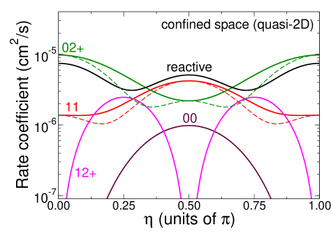
Figure 4: Same as Fig. 3 but in a confined quasi-2D geometry, using the same conditions as in Matsuda et al. (2020).

Finally, the overall reactive rate coefficients, while showing variations with the control parameter $\eta$, do not exhibit signatures of interferences, as it results in the sum of many state-to-state contributions of the possible reactive product pairs, included in a phenomenological way through $P^{re}_{\alpha lm_{l}}$ in Eq. (10) Wang and Quéméner (2015); SM . This is due to the fact that we cannot theoretically predict the individual state-to-state reactive rates, because we cannot predict the complex-valued $T$ matrix elements of each of the products pairs with our formalism. Only the norms of those elements are known and observed Liu et al. (2021), seemingly consistent with a statistical model González-Martínez et al. (2014); Bonnet and Larregaray (2020); Huang et al. (2021), but the individual phases remain still unknown. However, an experimental set-up as in Liu et al. (2021) combined with the one in Matsuda et al. (2020); Li et al. (2021), would be able to directly measure those state-to-state interfering reactive probabilities as a function of $\eta$. By fitting the experimental results, one could imagine to get back to all the state-to-state complex-valued $T$ matrix elements (including the phases) of the $\alpha=11$ and $\alpha=02+$ columns in Eq. (6). This is reminiscient of a “complete chemical experiment” Bohn et al. (2017) at ultracold temperature, here from an interferometry-type experiment between two collisional waves of matter, with the prospect of measuring all the scattering phase-shifts of a reaction.

In conclusion, we showed that a quantum-controlled microwave preparation of a dipolar molecule at a Förster resonance in an electric field, set the conditions for observing interferences between collisional waves and coherent control of their dynamics, in current ultracold molecular experiments. Evidences of constructive or destructive interferences are predicted to appear in the rate coefficients of two dipolar molecules measured in their first excited rotational state ($\alpha^{\prime}=11$) or in their ground and second excited rotational state ($\alpha^{\prime}=02+$), for different cases of confinements. The overall reactive rate coefficients do not exhibit signatures of interferences, but the state-to-state reactive rates are expected to do so. Future experimental observations of such individual rates in the distribution of the product pairs could be done combining the set-ups of Ref. Liu et al. (2021) and Refs. Matsuda et al. (2020); Li et al. (2021). This would be a signature of coherent control of ultracold chemistry at the state-to-state level. This study opens many interesting perspectives as coherent control could be used to enhance entanglement production of ultracold trapped pairs needed for many quantum physics applications, and to measure each individual state-to-state scattering phase shifts of a reaction envisioning “complete chemical experiments” at ultracold temperatures.

This work was supported by a grant overseen by the French National Research Agency (ANR) as part of the France 2030 program “Compétences et Métiers d’Avenir” within QuantEdu France project reference: ANR-22-CMA-0001 and by Quantum Saclay center.

Supplemental material

.1 Recoil energy and Doppler effect for a microwave transition

The energy and the momentum of a molecule are not conserved during a stimulated microwave process, the difference being given by the energy and momentum of the emitted/absorbed photon. Spontaneous emission processes can be neglected here for microwave transitions. Let’s consider a general case with a molecule $A$ in state $\ket{1}$ with wavevector $\vec{k}_{A,1}$ undergoing a stimulated emission process $\ket{1}\rightarrow\ket{0}$ in state $\ket{0}$ getting a wavevector $\vec{k}_{A,0}$, with a photon $a$ of energy $\hbar\omega_{a}$ and momentum $\vec{k}_{a}$. From conservation of energy, we have

$$\frac{\hbar^{2}k^{2}_{A,1}}{2m}+\varepsilon_{1}=\frac{\hbar^{2}k^{2}_{A,0}}{2m}+\varepsilon_{0}+\hbar\omega_{A}$$ (11)

where $\hbar\omega_{A}$ is the energy of the photon emitted by the molecule $A$. From conservation of momentum, we have

$$\hbar\vec{k}_{A,1}=\hbar\vec{k}_{A,0}+\hbar\vec{k}_{a}.$$ (12)

If we choose a space fixed frame such as the laboratory frame, we have using Eq. (12)

$$\frac{\hbar^{2}\vec{k}_{A,0}^{2}}{2m} = \frac{\hbar^{2}\big{(}\vec{k}_{A,1}-\vec{k}_{a}\big{)}^{2}}{2m}=E^{kin}_{A,1}+E^{r}_{a}-\hbar\,\vec{v}_{A,1}.\vec{k}_{a}=E^{kin}_{A,1}+E^{r}_{a}-2\,\cos\theta_{A,1}\sqrt{E^{kin}_{A,1}}\,\sqrt{E^{r}_{a}}$$ (13)

with the recoil energy defined as

$$E^{r}_{a}=\frac{\hbar^{2}k_{a}^{2}}{2m}=\frac{\hbar^{2}\omega_{a}^{2}}{2mc^{2}}=\hbar\omega_{a}\times\frac{\hbar\omega_{a}}{2mc^{2}}.$$ (14)

We used the fact that $\vec{v}_{A,1}=\frac{\hbar\vec{k}_{A,1}}{m}$ and $\frac{\hbar^{2}\vec{k}_{A,1}^{2}}{2m}=E^{kin}_{A,1}$. The kinetic energy of the molecule $A$ in state $\ket{0}$ is the sum of the kinetic energy of the molecule $A$ in state $\ket{1}$, the recoil energy $E^{r}_{a}$ and the Doppler effect term $-\hbar\,\vec{v}_{A,1}.\vec{k}_{a}$ (see for example Cohen-Tannoudji et al. (2019)). Using Eq. (11), we get that the energy of the emitted photon by molecule $A$ in the space-fixed frame (noted $\hbar\omega_{A}^{sf}$) should satisfy

$$\hbar\omega_{A}^{sf}=\varepsilon_{1}-\varepsilon_{0}-E^{r}_{a}+\hbar\,\vec{v}_{A,1}.\vec{k}_{a}.$$ (15)

Let’s also consider a general case with a molecule $B$ in state $\ket{1}$ with wavevector $\vec{k}_{B,1}$ undergoing a stimulated absorption process $\ket{1}\rightarrow\ket{2}$ in state $\ket{2}$ getting a wavevector $\vec{k}_{B,2}$, with a photon $b$ of energy $\hbar\omega_{b}$ and momentum $\vec{k}_{b}$. Similarly, we have

$$\frac{\hbar^{2}k^{2}_{B,2}}{2m}+\varepsilon_{2}=\frac{\hbar^{2}k^{2}_{B,1}}{2m}+\varepsilon_{1}+\hbar\omega_{B}$$ (16)

and

$$\hbar\vec{k}_{B,2}=\hbar\vec{k}_{B,1}+\hbar\vec{k}_{b}.$$ (17)

We deduce

$$\frac{\hbar^{2}\vec{k}_{B,2}^{2}}{2m} = \frac{\hbar^{2}\big{(}\vec{k}_{B,1}+\vec{k}_{b}\big{)}^{2}}{2m}=E^{kin}_{B,1}+E^{r}_{b}+\hbar\,\vec{v}_{B,1}.\vec{k}_{b}=E^{kin}_{B,1}+E^{r}_{b}+2\,\cos\theta_{B,1}\sqrt{E^{kin}_{B,1}}\,\sqrt{E^{r}_{b}}$$ (18)

and

$$\hbar\omega_{B}^{sf}=\varepsilon_{2}-\varepsilon_{1}+E^{r}_{b}+\hbar\,\vec{v}_{B,1}.\vec{k}_{b}$$ (19)

the energy of the photon absorbed by the molecule $B$ in the space-fixed frame. In this study at the Förster resonnance, we have $\varepsilon_{2}-\varepsilon_{1}=\varepsilon_{1}-\varepsilon_{0}\simeq k_{B}\times 200.6$ mK for ⁴⁰K⁸⁷Rb molecules. As the microwave processes are resonant ($\Delta=0$) and as the transitions $\ket{1}\rightarrow\ket{0}$ and $\ket{1}\rightarrow\ket{2}$ have the same energies, we have $\hbar\omega_{a}=\hbar\omega_{b}\simeq k_{B}\times 200.6$ mK ($\simeq h\times 4.2$ GHz). We can deduce that the ratio $\frac{\hbar\omega_{a,b}}{2mc^{2}}\simeq 7\ 10^{-17}$ in Eq. (14), so that $E^{r}_{a,b}\simeq 10^{-14}$ K. We can also deduce the effect of the Doppler effect characterized by the terms $2\,\sqrt{E^{kin}_{A,1}}\,\sqrt{E^{r}_{a}}=2\,\sqrt{E^{kin}_{B,1}}\,\sqrt{E^{r}_{b}}\simeq k_{B}\times 10^{-10}$ K in Eq. (13) or Eq. (18), choosing $E^{kin}_{A,1}=E^{kin}_{B,1}\simeq k_{B}\times 500$ nK and taking $|\cos\theta_{A,1}|=|\cos\theta_{B,1}|=1$. We can see that we can neglect both recoil energy and Doppler effect in this study when compared to the kinetic energies. In other words, the momentum of a microwave photon is small enough that it does not impact the one of the molecule when an emission or absorption takes place. This implies that the wavevector and kinetic energy of a molecule excited in state $\ket{2}$ or de-excited in state $\ket{0}$ are the same as a molecule in state $\ket{1}$, so that $\vec{k}_{2}\simeq\vec{k}_{0}\simeq\vec{k}_{1}$ and $\hbar^{2}k^{2}_{2}/2m\simeq\hbar^{2}k^{2}_{0}/2m\simeq\hbar^{2}k^{2}_{1}/2m$.

.2 Wavevectors of the center-of-mass and relative motions for the combined molecular states

Let’s consider now a given colliding pair with a molecule $A$ in state $i=0,1,2$ and a molecule $B$ in state $j=0,1,2$. The wavevectors for their center-of-mass and relative motion are given by

$$\vec{K}_{ij} =\vec{k}_{A,i}+\vec{k}_{B,j} \vec{k}_{ij} =\big{(}\vec{k}_{A,i}-\vec{k}_{B,j}\big{)}/2$$ (20)

starting from their individual wavevectors defined in the previous section. For $ij=11$, we have

$$\vec{K}_{11} =\vec{k}_{A,1}+\vec{k}_{B,1} \vec{k}_{11} =\big{(}\vec{k}_{A,1}-\vec{k}_{B,1}\big{)}/2$$ (21)

and for $ij=02$, we have

$$\vec{K}_{02} =\vec{k}_{A,0}+\vec{k}_{B,2}=\vec{k}_{A,1}-\vec{k}_{a}+\vec{k}_{B,1}+\vec{k}_{b}=\vec{K}_{11}+\vec{k}_{b}-\vec{k}_{a} \vec{k}_{02} =\big{(}\vec{k}_{A,0}-\vec{k}_{B,2}\big{)}/2=\vec{k}_{11}-\big{(}\vec{k}_{a}+\vec{k}_{b}\big{)}/2$$ (22)

using Eq. (12) and Eq. (17). Similarly, we have

$$\vec{K}_{00} =\vec{k}_{A,0}+\vec{k}_{B,0}=\vec{k}_{A,1}-\vec{k}_{a}+\vec{k}_{B,1}-\vec{k}_{a}=\vec{K}_{11}-2\vec{k}_{a} \vec{k}_{00} =\big{(}\vec{k}_{A,0}-\vec{k}_{B,0}\big{)}/2=\vec{k}_{11}$$

$$\vec{K}_{01} =\vec{k}_{A,0}+\vec{k}_{B,1}=\vec{k}_{A,1}-\vec{k}_{a}+\vec{k}_{B,1}=\vec{K}_{11}-\vec{k}_{a} \vec{k}_{01} =\big{(}\vec{k}_{A,0}-\vec{k}_{B,1}\big{)}/2=\vec{k}_{11}-\vec{k}_{a}/2$$

$$\vec{K}_{12} =\vec{k}_{A,1}+\vec{k}_{B,2}=\vec{k}_{A,1}+\vec{k}_{B,1}+\vec{k}_{b}=\vec{K}_{11}+\vec{k}_{b} \vec{k}_{12} =\big{(}\vec{k}_{A,1}-\vec{k}_{B,2}\big{)}/2=\vec{k}_{11}-\vec{k}_{b}/2$$

$$\vec{K}_{22} =\vec{k}_{A,2}+\vec{k}_{B,2}=\vec{k}_{A,1}+\vec{k}_{b}+\vec{k}_{B,1}+\vec{k}_{b}=\vec{K}_{11}+2\vec{k}_{b} \vec{k}_{22} =\big{(}\vec{k}_{A,2}-\vec{k}_{B,2}\big{)}/2=\vec{k}_{11}.$$ (23)

We can see that in a general case, if $\vec{k}_{a}=\vec{k}_{b}$, that is if the microwave source for the photons $a$ and $b$ is the same (same energy and same wavevector), becoming a unique source of photon, then $\vec{K}_{02}=\vec{K}_{11}$. The center-of-mass motions are then equal for these two types of pairs. If the recoil energy and the Doppler term can be neglected, it is also straightforward that all $\vec{K}_{ij}$ (noted $\vec{K}$ then) and $\vec{k}_{ij}$ (noted $\vec{k}$ then) are mainly identical. All pairs after the microwave preparation have mainly the same center-of-mass and collide with the same collision energy and wavevector as the initial colliding pair in state $\ket{11}$.

.3 Light-matter Hamiltonian. Preparation coefficients for an individual molecule

The total Hamiltonian describing the light-matter Hamiltonian is given by $H(t)=H_{0}+H^{\prime}(t)$. $H_{0}$ is the time-independent Hamiltonian of the unperturbated system, including its kinetic energy and its internal energy, with eigenfunctions $\ket{\bar{i}}\equiv\ket{i}e^{\text{i}\vec{k}_{i}.\vec{\rho}}$ associated to the eigenvalues $\hbar\omega_{i}=\hbar^{2}k^{2}_{i}/2m+\varepsilon_{i}$ at the Förster resonance. The three states taken into consideration are $i=0,1,2$. Higher states $i>2$ are higher in energy and never come into play in the process. The wavefunctions associated to each of these stationary states are given by $\ket{\Psi_{i}}=\ket{\bar{i}}e^{-\text{i}\omega_{i}t}$. $H^{\prime}(t)$ is the time-dependent Hamiltonian representing the usual light-matter interaction. Following the previous section, we will assume a unique photon of frequency $\omega_{p}=\omega_{a}=\omega_{b}$ and intensity defined by an ac electric field $E_{ac}$. We consider linear polarization. The Hamiltonian is given by $H^{\prime}(t)=-\vec{d}.\vec{E}_{ac}\cos(\omega_{p}t)=-\vec{d}.\vec{E}_{ac}\,(e^{+\text{i}\omega_{p}t}+e^{-\text{i}\omega_{p}t})/2$. The total Hamiltonian is given in the basis of the stationary states by Gaubatz et al. (1990); Bergmann et al. (1998); Vitanov et al. (2017)

$$\mathbf{H}(t) =\begin{pmatrix}\hbar\omega_{0}&-\frac{\hbar\Omega_{10}}{2}e^{i\omega_{p}t}&0\\ -\frac{\hbar\Omega_{10}}{2}e^{-i\omega_{p}t}&\hbar\omega_{1}&-\frac{\hbar\Omega_{12}}{2}e^{i\omega_{p}t}\\ 0&-\frac{\hbar\Omega_{12}}{2}e^{-i\omega_{p}t}&\hbar\omega_{2}\end{pmatrix}$$ (24)

where we defined the Rabi frequencies $\Omega_{10}=\tilde{d}^{1\leftrightarrow 0}\,E_{ac}/\hbar\equiv\Omega$, $\Omega_{12}=\tilde{d}^{1\leftrightarrow 2}\,E_{ac}/\hbar\equiv\chi\,\Omega$, and the generalized induced dipole moments $\tilde{d}^{1\leftrightarrow 0}=\bra{0}\vec{d}\ket{1}=\bra{1}\vec{d}\ket{0}$, $\tilde{d}^{1\leftrightarrow 2}=\bra{2}\vec{d}\ket{1}=\bra{1}\vec{d}\ket{2}$, computed for example in Lassablière and Quéméner (2022) at the Förster resonance. We also note $\Omega_{10}\equiv\Omega$ and $\Omega_{12}\equiv\chi\,\Omega$. Using now the usual dressed picture of a molecule with a photon for a ladder scheme, we get Vitanov et al. (2017)

$$\mathbf{H}(t) =\begin{pmatrix}\hbar\omega_{0}+\hbar\omega_{p}&-\frac{\hbar\Omega_{10}}{2}&0\\ -\frac{\hbar\Omega_{10}}{2}&\hbar\omega_{1}&-\frac{\hbar\Omega_{12}}{2}\\ 0&-\frac{\hbar\Omega_{12}}{2}&\hbar\omega_{2}-\hbar\omega_{p}\end{pmatrix}=\begin{pmatrix}0&-\frac{\hbar\Omega_{10}}{2}&0\\ -\frac{\hbar\Omega_{10}}{2}&-\hbar\Delta&-\frac{\hbar\Omega_{12}}{2}\\ 0&-\frac{\hbar\Omega_{12}}{2}&-2\hbar\Delta\end{pmatrix}\equiv\begin{pmatrix}0&-\frac{\hbar\Omega}{2}&0\\ -\frac{\hbar\Omega}{2}&-\hbar\Delta&-\chi\,\frac{\hbar\Omega}{2}\\ 0&-\chi\,\frac{\hbar\Omega}{2}&-2\hbar\Delta\end{pmatrix}.$$ (25)

We defined the detuning $\hbar\Delta=\hbar\omega_{p}-(\hbar\omega_{1}-\hbar\omega_{0})$ and used the fact that at the Förster resonance, we have $\hbar\omega_{2}-\hbar\omega_{1}$ = $\hbar\omega_{1}-\hbar\omega_{0}$ since we have $\varepsilon_{2}-\varepsilon_{1}$ = $\varepsilon_{1}-\varepsilon_{0}$ for the internal energies, and $\hbar^{2}k^{2}_{2}/2m\simeq\hbar^{2}k^{2}_{0}/2m\simeq\hbar^{2}k^{2}_{1}/2m$ for the kinetic energies. Because of $H^{\prime}(t)$, the general wavefunction becomes a linear combination of the stationnary states. It can also be recast in term of new eigenstates $\ket{a_{0,\pm}}$, the ones that diagonalize Eq. (25) when $\Delta=0$, the case studied in the paper. We have then

$$\ket{\Psi_{mol}}=\sum_{i=0}^{2}{c}_{i}\ket{\bar{i}}e^{-\text{i}\omega_{i}t}=\sum_{j=0,\pm}{c}_{a_{j}}\ket{a_{j}}e^{-\text{i}\omega^{a_{j}}t}$$ (26)

with Gaubatz et al. (1990)

$$\ket{a_{0}} =\cos\Theta\ket{\bar{0}}-\sin\Theta\ket{\bar{2}} \ket{a_{\pm}} =\frac{1}{\sqrt{2}}\bigg{(}\sin\Theta\ket{\bar{0}}\pm\ket{\bar{1}}+\cos\Theta\ket{\bar{2}}\bigg{)}.$$ (27)

The associated eigenvalues are

$$E^{a_{0}} =\hbar\omega^{a_{0}}=0 E^{a_{\pm}} =\hbar\omega^{a_{\pm}}=\pm\frac{\hbar}{2}\Omega_{RMS} \qquad\text{with}\qquad\Omega_{RMS} =\sqrt{\Omega_{10}^{2}+\Omega_{12}^{2}}=\Omega\sqrt{1+\chi^{2}}.$$ (28)

The angle $\Theta$ is defined as $\tan\Theta=\Omega_{10}/\Omega_{12}=1/\chi$. By solving the time-dependent Schrödinger equation using the basis of eigenstates Eq. (27) and the third term of Eq. (26), we found that $d{c}_{a_{j}}/dt=0$ so that ${c}_{a_{j}}$ are constants and independent of time. Using the initial conditions $c_{1}=1$, $c_{0}=0$, $c_{2}=0$ in Eq. (26) at $t=0$, and noting that $\ket{\bar{1}}=\{\ket{a_{+}}-\ket{a_{-}}\}/\sqrt{2}$ in Eq. (27), we found ${c}_{a_{0}}=0$, ${c}_{a_{\pm}}=\pm 1/{\sqrt{2}}$. From Eq. (27), we have the general relation

$$\begin{pmatrix}{c}_{a_{+}}\,e^{-\text{i}\omega^{a_{+}}t}\\ {c}_{a_{0}}\\ {c}_{a_{-}}\,e^{-\text{i}\omega^{a_{-}}t}\end{pmatrix}=M\begin{pmatrix}{c}_{0}\,e^{-\text{i}\omega_{0}t}\\ {c}_{1}\,\,e^{-\text{i}\omega_{1}t}\\ {c}_{2}\,e^{-\text{i}\omega_{2}t}\end{pmatrix}\equiv\begin{pmatrix}\frac{\sin\Theta}{\sqrt{2}}&\frac{1}{\sqrt{2}}&\frac{\cos\Theta}{\sqrt{2}}\\ \cos\Theta&0&-\sin\Theta\\ \frac{\sin\Theta}{\sqrt{2}}&-\frac{1}{\sqrt{2}}&\frac{\cos\Theta}{\sqrt{2}}\end{pmatrix}\begin{pmatrix}{c}_{0}\,e^{-\text{i}\omega_{0}t}\\ {c}_{1}\,\,e^{-\text{i}\omega_{1}t}\\ {c}_{2}\,e^{-\text{i}\omega_{2}t}\end{pmatrix}$$ (29)

and the inverse one

$$\begin{pmatrix}{c}_{0}\,e^{-\text{i}\omega_{0}t}\\ {c}_{1}\,\,e^{-\text{i}\omega_{1}t}\\ {c}_{2}\,e^{-\text{i}\omega_{2}t}\end{pmatrix}={M}^{-1}\begin{pmatrix}{c}_{a_{+}}\,e^{-\text{i}\omega^{a_{+}}t}\\ {c}_{a_{0}}\\ {c}_{a_{-}}\,e^{-\text{i}\omega^{a_{-}}t}\end{pmatrix}\equiv\begin{pmatrix}\frac{\sin\Theta}{\sqrt{2}}&\cos\Theta&\frac{\sin\Theta}{\sqrt{2}}\\ \frac{1}{\sqrt{2}}&0&-\frac{1}{\sqrt{2}}\\ \frac{\cos\Theta}{\sqrt{2}}&-\sin\Theta&\frac{\cos\Theta}{\sqrt{2}}\end{pmatrix}\begin{pmatrix}{c}_{a_{+}}\,e^{-\text{i}\omega^{a_{+}}t}\\ {c}_{a_{0}}\\ {c}_{a_{-}}\,e^{-\text{i}\omega^{a_{-}}t}\end{pmatrix}\\ =\begin{pmatrix}\frac{\sin\Theta}{\sqrt{2}}&\cos\Theta&\frac{\sin\Theta}{\sqrt{2}}\\ \frac{1}{\sqrt{2}}&0&-\frac{1}{\sqrt{2}}\\ \frac{\cos\Theta}{\sqrt{2}}&-\sin\Theta&\frac{\cos\Theta}{\sqrt{2}}\end{pmatrix}\begin{pmatrix}\frac{1}{\sqrt{2}}\,e^{-\text{i}\omega^{a_{+}}t}\\ 0\\ -\frac{1}{\sqrt{2}}\,e^{-\text{i}\omega^{a_{-}}t}\end{pmatrix}.$$ (30)

Then

$$\begin{pmatrix}{c}_{0}\,e^{-\text{i}\omega_{0}t}\\ {c}_{1}\,\,e^{-\text{i}\omega_{1}t}\\ {c}_{2}\,e^{-\text{i}\omega_{2}t}\end{pmatrix}=\begin{pmatrix}-\text{i}\sin\Theta\,\sin\bigg{(}\sqrt{1+\chi^{2}}\,\Omega t/2\bigg{)}\\ \cos\bigg{(}\sqrt{1+\chi^{2}}\,\Omega t/2\bigg{)}\\ -\text{i}\cos\Theta\,\sin\bigg{(}\sqrt{1+\chi^{2}}\,\Omega t/2\bigg{)}\end{pmatrix}.$$ (31)

At time $\tau$, we have then

$${c}_{0} =-\text{i}\sin\Theta\,\sin\eta\,e^{\text{i}\omega_{0}\tau} {c}_{1} =\cos\eta\,e^{\text{i}\omega_{1}\tau} {c}_{2} =-\text{i}\cos\Theta\,\sin\eta\,e^{\text{i}\omega_{2}\tau}$$ (32)

using the notation $\eta=\sqrt{1+\chi^{2}}\,\Omega\tau/2$. If we set ${c}_{i}=C_{i}\,e^{\text{i}\omega_{i}\tau}$, we identify

$${C}_{0} =-\text{i}\sin\Theta\sin\eta {C}_{1} =\cos\eta {C}_{2} =-\text{i}\cos\Theta\sin\eta.$$ (33)

.4 Preparation coefficients for the combined molecular states

Using Eq. 1 of the paper, we get for the overall incident collisional wavefunction between two molecules

$$\ket{\Psi_{col}^{inc}} = \ket{\Psi_{mol}}\otimes\ket{\Psi_{mol}}$$ (34)

$$= C_{0}^{2}e^{i\left((\vec{k}_{0}+\vec{k}_{0}).\vec{\rho}-(\omega_{0}+\omega_{0})(t-\tau)\right)}\ket{00}+C_{1}^{2}e^{i\left((\vec{k}_{1}+\vec{k}_{1}).\vec{\rho}-(\omega_{1}+\omega_{1})(t-\tau)\right)}\ket{11}$$

$$+ C_{2}^{2}e^{i\left((\vec{k}_{2}+\vec{k}_{2}).\vec{\rho}-(\omega_{2}+\omega_{2})(t-\tau)\right)}\ket{22}+C_{0}C_{1}e^{i\left((\vec{k}_{0}+\vec{k}_{1}).\vec{\rho}-(\omega_{0}+\omega_{1})(t-\tau)\right)}\left(\ket{01}+\ket{10}\right)$$

$$+ C_{1}C_{2}e^{i\left((\vec{k}_{1}+\vec{k}_{2}).\vec{\rho}-(\omega_{1}+\omega_{2})(t-\tau)\right)}\left(\ket{12}+\ket{21}\right)+C_{0}C_{2}e^{i\left((\vec{k}_{0}+\vec{k}_{2}).\vec{\rho}-(\omega_{0}+\omega_{2})(t-\tau)\right)}\left(\ket{02}+\ket{20}\right).$$

Since these states need to be properly symmetrized under exchange of identical particles and since we start with identical molecules in indistinguishable states, only symmetric states are involved in the dynamics Wang and Quéméner (2015). These symmetric states are defined as $\ket{ij+}=\frac{1}{\sqrt{2(1+\delta_{i,j})}}\left(\ket{ij}+\ket{ji}\right)$. Then Eq. (34) is rewritten

$$\ket{\Psi_{col}^{inc}} = C_{0}^{2}e^{i\left((\vec{k}_{0}+\vec{k}_{0}).\vec{\rho}-(\omega_{0}+\omega_{0})(t-\tau)\right)}\ket{00+}+C_{1}^{2}e^{i\left((\vec{k}_{1}+\vec{k}_{1}).\vec{\rho}-(\omega_{1}+\omega_{1})(t-\tau)\right)}\ket{11+}$$ (35)

$$+ C_{2}^{2}e^{i\left((\vec{k}_{2}+\vec{k}_{2}).\vec{\rho}-(\omega_{2}+\omega_{2})(t-\tau)\right)}\ket{22+}+\sqrt{2}\,C_{0}C_{1}\,e^{i\left((\vec{k}_{0}+\vec{k}_{1}).\vec{\rho}-(\omega_{0}+\omega_{1})(t-\tau)\right)}\ket{01+}$$

$$+ \sqrt{2}\,C_{1}C_{2}\,e^{i\left((\vec{k}_{1}+\vec{k}_{2}).\vec{\rho}-(\omega_{1}+\omega_{2})(t-\tau)\right)}\ket{12+}+\sqrt{2}\,C_{0}C_{2}\,e^{i\left((\vec{k}_{0}+\vec{k}_{2}).\vec{\rho}-(\omega_{0}+\omega_{2})(t-\tau)\right)}\ket{02+}.$$

In the paper, we omit the plus sign for the states $\ket{00+}$, $\ket{11+}$ $\ket{22+}$, as they are obviously symmetric under exchange of particles. Then

$$C_{00} =C_{0}^{2} C_{11} =C_{1}^{2} C_{22} =C_{2}^{2}$$

$$C_{01} =\sqrt{2}\,C_{0}C_{1} C_{12} =\sqrt{2}\,C_{1}C_{2} C_{02} =\sqrt{2}\,C_{0}C_{2}.$$ (36)

.5 Overall loss rate coefficient and probabilities

From Eq. 6 of the paper, we can make the link between the $T$ matrix and the $S$ matrix for the interference term

$$T^{qs}_{\alpha^{\prime}l^{\prime}m_{l}^{\prime},11/02+\,lm_{l}} = C_{11}T_{\alpha^{\prime}l^{\prime}m_{l}^{\prime},11\,lml}+C_{02+}T_{\alpha^{\prime}l^{\prime}m_{l}^{\prime},02+\,lm_{l}}$$ (37)

$$= C_{11}(S_{\alpha^{\prime}l^{\prime}m_{l}^{\prime},11\,lml}-\delta_{\alpha^{\prime}l^{\prime}m_{l}^{\prime},11\,lml})+C_{02+}(S_{\alpha^{\prime}l^{\prime}m_{l}^{\prime},02+\,lml}-\delta_{\alpha^{\prime}l^{\prime}m_{l}^{\prime},02+\,lml})$$

$$= (C_{11}S_{\alpha^{\prime}l^{\prime}m_{l}^{\prime},11\,lml}+C_{02+}S_{\alpha^{\prime}l^{\prime}m_{l}^{\prime},02+\,lml})-(C_{11}\delta_{\alpha^{\prime}l^{\prime}m_{l}^{\prime},11\,lml}+C_{02+}\delta_{\alpha^{\prime}l^{\prime}m_{l}^{\prime},02+\,lml}).$$

This defines a new expression for the scattering matrix for the interference term

$$S^{qs}_{\alpha^{\prime}l^{\prime}m_{l}^{\prime},11/02+\,lm_{l}} = C_{11}S_{\alpha^{\prime}l^{\prime}m_{l}^{\prime},11\,lml}+C_{02+}S_{\alpha^{\prime}l^{\prime}m_{l}^{\prime},02+\,lm_{l}}.$$ (38)

For the satellite terms we have simply

$$S^{qs}_{\alpha^{\prime}l^{\prime}m_{l}^{\prime},\alpha\,lm_{l}} =C_{\alpha}S_{\alpha^{\prime}l^{\prime}m_{l}^{\prime},\alpha\,lml}.$$ (39)

The modulus square of the $S^{qs}$ matrix elements are associated to the probabilities, the sum of which for a given column should give unity. Let’s check the conservation of these associated probabilities. For a given column of the $S^{qs}$ matrix for a given $l,m_{l}$, and for all the states $\alpha^{\prime}$ (spending all reactants or products), we have for the interference term

$$\sum_{\alpha^{\prime},l^{\prime},m_{l}^{\prime}}|S^{qs}_{\alpha^{\prime}\,l^{\prime}\,m_{l}^{\prime},11/02+\,l\,m_{l}}|^{2} = \sum_{\alpha^{\prime},l^{\prime},m_{l}^{\prime}}|C_{11}\,S_{\alpha^{\prime}\,l^{\prime}\,m_{l}^{\prime},11\,l\,m_{l}}+C_{02+}\,S_{\alpha^{\prime}\,l^{\prime}\,m_{l}^{\prime},02+\,l\,m_{l}}|^{2}$$ (40)

$$= \sum_{\alpha^{\prime},l^{\prime},m_{l}^{\prime}}\bigg{(}|C_{11}|^{2}\,|S_{\alpha^{\prime}\,l^{\prime}\,m_{l}^{\prime},11\,l\,m_{l}}|^{2}+|C_{02+}|^{2}\,|S_{\alpha^{\prime}\,l^{\prime}\,m_{l}^{\prime},02+\,l\,m_{l}}|^{2}$$

$$+ C_{11}^{*}\,C_{02+}\,[S_{\alpha^{\prime}\,l^{\prime}\,m_{l}^{\prime},11\,l\,m_{l}}]^{*}\,S_{\alpha^{\prime}\,l^{\prime}\,m_{l}^{\prime},02+\,l\,m_{l}}+C_{02+}^{*}\,C_{11}\,[S_{\alpha^{\prime}\,l^{\prime}\,m_{l}^{\prime},02+\,l\,m_{l}}]^{*}\,S_{\alpha^{\prime}\,l^{\prime}\,m_{l}^{\prime},11\,l\,m_{l}}\bigg{)}$$

$$= |C_{11}|^{2}\,\sum_{\alpha^{\prime},l^{\prime},m_{l}^{\prime}}\,|S_{\alpha^{\prime}\,l^{\prime}\,m_{l}^{\prime},11\,l\,m_{l}}|^{2}+|C_{02+}|^{2}\,\sum_{\alpha^{\prime},l^{\prime},m_{l}^{\prime}}\,|S_{\alpha^{\prime}\,l^{\prime}\,m_{l}^{\prime},02+\,l\,m_{l}}|^{2}$$

$$= |C_{11}|^{2}+|C_{02+}|^{2}$$

$$\equiv P^{el,qs}_{11/02+\,l\,m_{l}}+P^{in,qs}_{11/02+\,l\,m_{l}}+P^{re,qs}_{11/02+\,l\,m_{l}}.$$

This is equal to the sum of the elastic $P^{el,qs}$, inelastic $P^{in,qs}$ and reactive $P^{re,qs}$ probabilities starting in the interfering state $11/02+$. We used the fact that a $S$ matrix is unitary so that we have

$$\sum_{\alpha^{\prime},l^{\prime},m_{l}^{\prime}}[S_{\alpha^{\prime}\,l^{\prime}\,m_{l}^{\prime},11\,l\,m_{l}}]^{*}\,S_{\alpha^{\prime}\,l^{\prime}\,m_{l}^{\prime},02+\,l\,m_{l}} = \sum_{\alpha^{\prime},l^{\prime},m_{l}^{\prime}}[S_{\alpha^{\prime}\,l^{\prime}\,m_{l}^{\prime},02+\,l\,m_{l}}]^{*}\,S_{\alpha^{\prime}\,l^{\prime}\,m_{l}^{\prime},11\,l\,m_{l}}=0$$

$$\sum_{\alpha^{\prime},l^{\prime},m_{l}^{\prime}}|S_{\alpha^{\prime}\,l^{\prime}\,m_{l}^{\prime},11\,l\,m_{l}}|^{2} = \sum_{\alpha^{\prime},l^{\prime},m_{l}^{\prime}}|S_{\alpha^{\prime}\,l^{\prime}\,m_{l}^{\prime},02+\,l\,m_{l}}|^{2}=1.$$ (41)

Similarly for the satellite terms, we have

$$\sum_{\alpha^{\prime},l^{\prime},m_{l}^{\prime}}|S^{qs}_{\alpha^{\prime}\,l^{\prime}\,m_{l}^{\prime},\alpha\,l\,m_{l}}|^{2} = |C_{\alpha}|^{2}\equiv P^{el,qs}_{\alpha\,l\,m_{l}}+P^{in,qs}_{\alpha\,l\,m_{l}}+P^{re,qs}_{\alpha\,l\,m_{l}}.$$ (42)

This is equal to the sum of the elastic $P^{el,qs}$, inelastic $P^{in,qs}$ and reactive $P^{re,qs}$ probabilities starting in the satellite states $\alpha=00,01+,12+,22$. If we sum all of those interference and satellite probabilities for a given $l,m_{l}$ over $\alpha=11/02+,00,01+,12+,22$, we have then that

$$\sum_{\alpha}^{*}\,\sum_{\alpha^{\prime},l^{\prime},m_{l}^{\prime}}|S^{qs}_{\alpha^{\prime}\,l^{\prime}\,m_{l}^{\prime},\alpha\,l\,m_{l}}|^{2} = \sum_{\alpha}^{*}\,|C_{\alpha}|^{2}=|C_{0}|^{4}+|C_{1}|^{4}+|C_{2}|^{4}+2|C_{0}|^{2}|C_{1}|^{2}+2|C_{1}|^{2}|C_{2}|^{2}+2|C_{0}|^{2}|C_{2}|^{2}$$ (43)

$$= (|C_{0}|^{2}+|C_{1}|^{2}+|C_{2}|^{2})^{2}=1$$

where we used Eq. (.4) and Eq. (33). We then checked that the new expression of the $S$ matrices in Eq. (38) provides a sum of all probabilities of unity (for a given $l,m_{l}$), as it should be.

Among all the states $\alpha^{\prime}$, we don’t have information on those which correspond to the products of the reaction. Instead, the computed $S$ matrix is sub-unitary (due to an appropriate short-range absorbing boundary condition as explained in Wang and Quéméner (2015)) so that the difference with unitarity provides the overall phenomenological reactive probability. Then for a given $\alpha\,l\,m_{l}$, we have instead for the interference term

$$\sum^{el+in}_{\alpha^{\prime},l^{\prime},m_{l}^{\prime}}|S^{qs}_{\alpha^{\prime}\,l^{\prime}\,m_{l}^{\prime},11/02+\,l\,m_{l}}|^{2} \equiv P^{el,qs}_{11/02+\,l\,m_{l}}+P^{in,qs}_{11/02+\,l\,m_{l}}$$ (44)

$$= \sum^{el+in}_{\alpha^{\prime},l^{\prime},m_{l}^{\prime}}|C_{11}\,S_{\alpha^{\prime}\,l^{\prime}\,m_{l}^{\prime},11\,l\,m_{l}}+C_{02+}\,S_{\alpha^{\prime}\,l^{\prime}\,m_{l}^{\prime},02+\,l\,m_{l}}|^{2}$$

$$= \sum^{el+in}_{\alpha^{\prime},l^{\prime},m_{l}^{\prime}}\bigg{(}|C_{11}|^{2}\,|S_{\alpha^{\prime}\,l^{\prime}\,m_{l}^{\prime},11\,l\,m_{l}}|^{2}+|C_{02+}|^{2}\,|S_{\alpha^{\prime}\,l^{\prime}\,m_{l}^{\prime},02+\,l\,m_{l}}|^{2}$$

$$+ C_{11}^{*}\,C_{02+}\,[S_{\alpha^{\prime}\,l^{\prime}\,m_{l}^{\prime},11\,l\,m_{l}}]^{*}\,S_{\alpha^{\prime}\,l^{\prime}\,m_{l}^{\prime},02+\,l\,m_{l}}+C_{02+}^{*}\,C_{11}\,[S_{\alpha^{\prime}\,l^{\prime}\,m_{l}^{\prime},02+\,l\,m_{l}}]^{*}\,S_{\alpha^{\prime}\,l^{\prime}\,m_{l}^{\prime},11\,l\,m_{l}}\bigg{)}$$

$$= |C_{11}|^{2}\,\sum^{el+in}_{\alpha^{\prime},l^{\prime},m_{l}^{\prime}}\,|S_{\alpha^{\prime}\,l^{\prime}\,m_{l}^{\prime},11\,l\,m_{l}}|^{2}+|C_{02+}|^{2}\,\sum^{el+in}_{\alpha^{\prime},l^{\prime},m_{l}^{\prime}}\,|S_{\alpha^{\prime}\,l^{\prime}\,m_{l}^{\prime},02+\,l\,m_{l}}|^{2}$$

$$= |C_{11}|^{2}\,(P^{el}_{11\,l\,m_{l}}+P^{in}_{11\,l\,m_{l}})+|C_{02+}|^{2}\,(P^{el}_{02+\,l\,m_{l}}+P^{in}_{02+\,l\,m_{l}})$$

$$= |C_{11}|^{2}\,(1-P^{re}_{11\,l\,m_{l}})+|C_{02+}|^{2}\,(1-P^{re}_{02+\,l\,m_{l}})$$

$$= |C_{11}|^{2}+|C_{02+}|^{2}-|C_{11}|^{2}\,P^{re}_{11\,l\,m_{l}}-|C_{02+}|^{2}\,P^{re}_{02+\,l\,m_{l}}$$

where the special sum indicates that the sum on $\alpha^{\prime}$ is done on the elastic and inelastic states only. We can then identify

$$P^{re,qs}_{11/02+\,l\,m_{l}}=|C_{11}|^{2}\,P^{re}_{11\,l\,m_{l}}+|C_{02+}|^{2}\,P^{re}_{02+\,l\,m_{l}}$$ (45)

from the fact that $P^{el,qs}_{11/02+\,l\,m_{l}}+P^{in,qs}_{11/02+\,l\,m_{l}}+P^{re,qs}_{11/02+\,l\,m_{l}}=|C_{11}|^{2}+|C_{02+}|^{2}$. For the satellite terms, we have

$$\sum^{el+in}_{\alpha^{\prime},l^{\prime},m_{l}^{\prime}}|S^{qs}_{\alpha^{\prime}\,l^{\prime}\,m_{l}^{\prime},\alpha\,l\,m_{l}}|^{2} \equiv P^{el,qs}_{\alpha\,l\,m_{l}}+P^{in,qs}_{\alpha\,l\,m_{l}}=\sum^{el+in}_{\alpha^{\prime},l^{\prime},m_{l}^{\prime}}|C_{\alpha}\,S_{\alpha^{\prime}\,l^{\prime}\,m_{l}^{\prime},\alpha\,l\,m_{l}}|^{2}=|C_{\alpha}|^{2}\,(P^{el}_{\alpha\,l\,m_{l}}+P^{in}_{\alpha\,l\,m_{l}})=|C_{\alpha}|^{2}\,(1-P^{re}_{\alpha\,l\,m_{l}}).$$

Then we identify

$$P^{re,qs}_{\alpha\,l\,m_{l}}=|C_{\alpha}|^{2}\,P^{re}_{\alpha\,l\,m_{l}}$$ (46)

from the fact that $P^{el,qs}_{\alpha\,l\,m_{l}}+P^{in,qs}_{\alpha\,l\,m_{l}}+P^{re,qs}_{\alpha\,l\,m_{l}}=|C_{\alpha}|^{2}$.