Preprint nos. NJU-INP 082/23, USTC-ICTS/PCFT-23-40
Nucleon to $\Delta$ axial and pseudoscalar transition form factors

Abstract

A symmetry-preserving continuum approach to the calculation of baryon properties in relativistic quantum field theory is used to predict all form factors associated with nucleon–to–$\Delta$ axial and pseudoscalar transition currents, thereby unifying them with many additional properties of these and other baryons. The new parameter-free predictions can serve as credible benchmarks for use in analysing existing and anticipated data from worldwide efforts focused on elucidation of $\nu$ properties.

1. Introduction — With the discovery of neutrino ($\nu$) masses twenty-five years ago [1, 2, 3], science acquired tangible evidence of phenomena that lie beyond the Standard Model of particle physics (SM). With such motivation, precision measurements of $\nu$, $\bar{\nu}$ (antineutrino) properties are today amongst the top priorities in fundamental physics [4, 5, 6, 7, 8, 9, 10, 11].

Known neutrinos are very weakly interacting; so, their detection requires excellent understanding of detector responses to $\nu$ passage. The array of interactions that can occur depends strongly on $\nu$ energy. At low energies, elastic scattering on entire nuclei dominates; whereas at high energies, individual neutrons and protons (nucleons) are resolved and deep inelastic $\nu$-parton scatterings take place. (Partons are the degrees-of-freedom used to define quantum chromodynamics – QCD, i.e., the SM theory of strong interactions.) Yet another class of reactions is important in few-GeV reactor-based $\nu$ experiments, viz. inelastic processes on single or small clusters of nucleons, which produce a range of excited-nucleon final states.

To some extent, the required cross-sections can be determined in dedicated $\nu$ scattering experiments. However, reliable strong interaction theory predictions are equally important. In this context, results for nucleon ($N$) electroweak elastic and transition form factors become critical to interpreting modern $\nu$ oscillation experiments [12, 13, 14, 15]. Recognising this, the past five years have seen a focus on calculating the form factors associated with elastic $\nu N$ scattering using both continuum and lattice Schwinger function methods [16, 17, 18, 19, 20].

However, as noted above, inelastic processes are also crucial to understanding existing and anticipated experiments. The most significant of these are excitations of the $\Delta$-resonance via, e.g., $\nu_{\ell}N\to\ell\Delta$ and $\nu_{\ell}N\to\ell(\pi N\to\Delta)$, where $\ell$ is a light lepton and the second process involves the $\pi$-meson [21, 22]. Only one set of related calculations exists [23, 24]. They were obtained using lattice-QCD (lQCD) with quark current masses that produce a pion mass-squared $m_{\pi}^{2}\gtrsim 5(m_{\pi}^{\rm empirical})^{2}$, $m_{\pi}^{\rm empirical}=0.135\,$GeV. Lacking further studies, challenges remain, like extending computations to $m_{\pi}^{\rm empirical}$ and significantly reducing all uncertainties.

Hitherto, there have been no more recent predictions. We address that lack herein, employing a continuum approach to the baryon bound-state problem that has widely been used with success [25, 26, 27, 28]. Of particular relevance are its unifying predictions for $N$ and $\Delta$-baryon elastic weak-interaction form factors [16, 17, 29]. Where comparisons with experiment and results obtained using other robust tools are available, there is agreement.

2. Axial and pseudoscalar currents — Weak $N\to\Delta$ transitions are described by the matrix element

$${\mathcal{J}}_{5\mu}^{j}(K,Q ):=\langle\Delta(P_{f};s_{f})|{\mathcal{A}}^{j}_{5\mu}(0)|N(P_{i};s_{i})\rangle$$ (1a)

$$=\bar{u}_{\alpha}(P_{f};s_{f})\Gamma_{5\mu,\alpha}^{j}(K,Q)u(P_{i};s_{i})\,,$$ (1b)

where $P_{i,j}(s_{i,j})$ are the momenta (spins) of the incoming nucleon and outgoing $\Delta$, respectively, which are on-shell: $P_{i,f}^{2}=-m_{N,\Delta}^{2}$; and $K=(P_{f}+P_{i})/2$, $Q=P_{f}-P_{i}$. Isospin symmetry is assumed throughout [30]; and the on-shell baryons are described by Dirac and Rarita-Schwinger spinors, respectively – see Ref. [31, Appendix B] for details. Introducing the column vector $\psi={\rm column}[u,d]$, with $u$, $d$ being the two light-flavour quark fields, then the axial current operator may be written ${\mathcal{A}}^{j}_{5\mu}(x)=\bar{\psi}(x)\frac{\tau^{j}}{2}\gamma_{5}\gamma_{\mu}\psi(x)$, in which the isospin structure is expressed via the Pauli matrices $\{\tau^{j}|j=1,2,3\}$.

Owing to the assumed isospin symmetry, a complete characterisation of $N\to\Delta$ weak transitions can be achieved by focusing solely on the neutral current ($j=3$) $p\to\Delta^{+}$ transition, in which case the vertex is typically written in the following form [32, 33]:

$$\Gamma_{5\mu,\alpha}^{3}(K,Q) =\sqrt{\tfrac{2}{3}}\bigg{[}i(\gamma_{\mu}Q_{\alpha}-\delta_{\mu\alpha}\not{Q})C^{A}_{3}(Q^{2})/m_{N}$$

$$-(\delta_{\mu\alpha}(P_{f}\cdot Q)-{P_{f}}_{\mu}Q_{\alpha})C^{A}_{4}(Q^{2})/m_{N}^{2}$$

$$+\delta_{\mu\alpha}C^{A}_{5}(Q^{2})-Q_{\mu}Q_{\alpha}C^{A}_{6}(Q^{2})/m_{N}^{2}\bigg{]}\,,$$ (2)

where $C^{A}_{3,4,5,6}$ are the four Poincaré-invariant transition form factors and $\sqrt{2/3}$ is the isospin coefficient.

The related pseudoscalar transition matrix element is

$${\mathcal{J}}_{5}^{j}(K,Q )=\langle\Delta(P_{f};s_{f})|{\mathcal{P}}^{j}_{5}(0)|N(P_{i};s_{i})\rangle$$ (3a)

$$=\bar{u}_{\alpha}(P_{f};s_{f})\Gamma_{5,\alpha}^{j}(Q)u(P_{i};s_{i})\,,$$ (3b)

where ${\mathcal{P}}^{j}_{5}(x)=\bar{\psi}(x)\frac{\tau^{j}}{2}\gamma_{5}\psi(x)$. For the neutral current:

$$\Gamma_{5,\alpha}^{3}(Q) =\sqrt{\tfrac{2}{3}}i\frac{Q_{\alpha}}{4m_{N}}\frac{m_{\pi}^{2}}{Q^{2}+m_{\pi}^{2}}\frac{f_{\pi}}{m_{q}}G_{\pi N\Delta}(Q^{2})\,.$$ (4)

Here, $G_{\pi N\Delta}$ is the pseudoscalar transition form factor, $m_{q}$ is the light-quark current-mass, and $f_{\pi}=0.092\,$GeV is the pion leptonic decay constant [34].

Using the PCAC (partially conserved axial current) identity [30]: $\partial_{\mu}{\mathcal{A}}^{j}_{5\mu}(x)+2m_{q}{\mathcal{P}}^{j}_{5}(x)=0$, one obtains the following “off-diagonal” PCAC relation:

$$C^{A}_{5}(Q^{2})-\frac{Q^{2}}{m_{N}^{2}}C^{A}_{6}(Q^{2})=\frac{f_{\pi}m_{\pi}^{2}/[2m_{N}]}{Q^{2}+m_{\pi}^{2}}G_{\pi N\Delta}(Q^{2})\,.$$ (5)

Drawing a parallel with the nucleon [16], $C^{A}_{5}$ is kindred to the nucleon’s axial form factor, $G_{A}$, and $C^{A}_{6}$ to its induced-pseudoscalar form factor, $G_{P}$. Since $\left.Q^{2}C^{A}_{6}(Q^{2})\right|_{Q^{2}=0}=0$, one immediately obtains the off-diagonal Goldberger-Treiman (GT) relation

$$2m_{N}C^{A}_{5}(0)=f_{\pi}G_{\pi N\Delta}(0)\,.$$ (6)

As consequences of chiral symmetry and its breaking pattern, only frameworks preserving Eqs. (5), (6) are viable.

3. Baryon structure — The structure of any given baryon can be described by a Faddeev amplitude, obtained from a Poincaré-covariant Faddeev equation that sums all possible exchanges and interactions which can occur between the three dressed-quarks that characterise its valence content. Studies of the associated scattering problem reveal that there is no interaction contribution from the diagram in which each leg of the three-gluon vertex ($3g$V) is attached to a separate quark [26, Eq. (2.2.10)]. Thus, whilst the $3g$V is a primary factor in generating the process-independent QCD effective charge [35, 36], its role within baryons is largely to produce tight quark + quark (diquark) correlations. Consequently, the baryon bound-state problem may reliably be transformed [37, 38, 39] into solving the homogeneous matrix equation in Fig. 1.

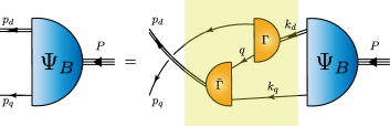
Figure 1: Faddeev integral equation, whose solution is the Poincaré-covariant matrix-valued function $\Psi_{B}$, the Faddeev amplitude for a baryon $B$ with total momentum $P=p_{q}+p_{d}$. Legend. Shaded box – Faddeev kernel; single line – dressed-quark propagator; $\Gamma$ – diquark correlation amplitude; and double line – diquark propagator. Only isoscalar-scalar diquarks, $[ud]$, and isovector–axialvector diquarks, $\{uu\}$, $\{ud\}$, $\{dd\}$ play a material role in nucleons and $\Delta$-baryons [26].

Each line and vertex in Fig. 1 is specified in Ref. [16], which delivers parameter-free predictions for the nucleon $G_{A,P}$ form factors and unifies them with the pion-nucleon form factor, $G_{\pi NN}$. A key to the success of that study is a sound expression of emergent hadron mass and its corollaries [40, 41, 42, 27, 43, 44, 45], such as a running light-quark mass whose value at infrared momenta, $M_{D}\approx 0.4\,$GeV, defines the natural magnitude for mass-dimensioned quantities in the light-quark sector of the Standard Model. Associated mass-scales for the isoscalar-scalar and isovector-axialvector diquarks are [in GeV]:

$$m_{[ud]}=0.80\,,\,\,\,m_{\{uu\}}=m_{\{ud\}}=m_{\{dd\}}=0.89\,.$$ (7)

In computing all transition form factors, we follow Refs. [16, 17, 29]: they are obtained from the nucleon elastic weak form factor expressions by replacing all inputs connected with the final state by those for the $\Delta$-baryon. The normalisations of the $N$ and $\Delta$ Faddeev amplitudes are available from Refs. [16, 29]. (The interaction current is included with the supplemental material.)

4. Dominant $N\to\Delta$ transition axial form factors — $C^{A}_{5,6}$ in Eq. (2) are dominant in the axial transition current. Our prediction for $C^{A}_{5}(x=Q^{2}/\bar{m}^{2})$, $\bar{m}=[m_{N}+m_{\Delta}]/2$, is drawn in Fig. 2A. On the domain depicted, $C^{A}_{5}(x)$ can fairly be interpolated using a dipole characterised by the $x=0$ value and axial mass listed in the first row of Table 1. The $x=0$ value is $0.94(5)$-times the prediction for $g_{A}$, the nucleon axial coupling, as calculated using the same framework; and the axial mass is $0.95(3)$-times the analogous scale in a dipole representation of $G_{A}(x)$, the nucleon axial form factor, viz. the axial transition form factor is softer, something also found in a coupled channels analysis of axial $N\to\Delta$ transitions [21].

The reported uncertainty in our predictions expresses the impact of $\pm 5\%$ variations of the diquark masses in Eq. (7). The results obtained from independent variations are combined with weight fixed by the relative strength of scalar $(0^{+})$ and axialvector $(1^{+})$ diquark contributions to $C^{A}_{5}(0)$, i.e., approximately $4$:$1$. Like the nucleon case [16, 17], the $0^{+}$ and $1^{+}$ mass variations interfere destructively, e.g., reducing $m_{[ud]}$ increases $C^{A}_{5}(0)$, whereas $C^{A}_{5}(0)$ decreases with the same change in $m_{1^{+}}$.

  A

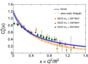
  B

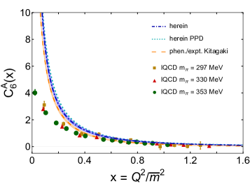
Figure 2: Panel A. $C^{A}_{5}$ calculated herein – blue curve within lighter blue uncertainty band; and empirical result [46, Kitagaki] – dashed orange curve within uncertainty band. Panel B. $C^{A}_{6}$ calculated herein – dot-dashed blue curve within uncertainty band; dotted cyan curve – PPD approximation, Eq. (9), using our prediction for $C^{A}_{5}(x)$; and dashed orange curve within uncertainty band – PPD approximation obtained with empirical result [46] for $C^{A}_{5}(x)$. Both panels: lQCD [23, 24] – hybrid (HYB) [green circles – $m_{\pi}=353$ MeV] and domain wall fermions (DWF) [gold squares – $m_{\pi}=297$ MeV, red triangles – $m_{\pi}=330$ MeV]. (Parametrisations of our form factor predictions are provided in the supplemental material.)

In phenomenology, following Ref. [47], it has been common to represent $C^{A}_{5}$ as follows [46]:

$$C^{A}_{5}(Q^{2})=C^{A}_{5}(0)\frac{[1+a_{5}Q^{2}/(b_{5}+Q^{2})]}{(1+Q^{2}/\tilde{m}_{A}^{2})^{2}}\,,$$ (8)

where $C^{A}_{5}(0)=1.2$, $a_{5}=-1.21$, $b_{5}=2\,$GeV² are parameters discussed in Ref. [47]. The value of $C^{A}_{5}(0)$ is an estimate based on the off-diagonal GT relation – Eq. (6). Using Eq. (8) and the same functional form for $C^{A}_{3,4,6}$, then a fit to $\nu d\to\mu^{-}\Delta^{++}n$ bubble chamber data yielded the value of $\tilde{m}_{A}$ in Table 1.

Table 1: Selected characteristics of $C^{A}_{5}$ compared with combined phenomenology and experiment [46] and other available calculations [23, 24]. ($2\bar{m}=m_{N}+m_{\Delta}$.)

	$C^{A}_{5}(0)$	$\tilde{m}_{A}/\bar{m}$
Herein	$1.16^{+0.09}_{-0.03}$	$1.01(2)$
Phenomenology/Empirical [46]	$1.2$	$1.18(8)$
Phenomenology/Empirical (dipole)	$1.2$	$0.88(4)$
lQCD [23] $m_{\pi}=353$ MeV	$0.90(1)$	$1.32(3)$
lQCD [24] $m_{\pi}=297$ MeV	$0.94(6)$	$1.32(13)$
lQCD [24] $m_{\pi}=330$ MeV	$0.97(3)$	$1.23(5)$

Taken at face value, this result is $1.34(17)$-times that which some phenomenological estimates now associate with the nucleon axial form factor [48]. However, as noted above, such estimates are based on dipole parametrisations. If one recasts Eq. (8) as a dipole, then the empirical fit corresponds to $\tilde{m}_{A}=1.01(5)m_{N}=0.878(41)\bar{m}$ – we have listed this value in Row 3 of Table 1. Using an ${\mathpzc L}_{1}$ measure, then, on the phenomenological fitting domain $Q^{2}\in[0,3]\,$GeV², the curves thus obtained agree with the original parametrisations to within 7.6(1.1)%. This dipole mass scale is $0.70(3)$-times that associated with the nucleon $G_{A}$.

Our prediction for $C^{A}_{5}$ in Fig. 2A is contrasted therein with a phenomenological/empirical result [46] and lQCD computations [23, 24]. Allowing for the constraint imposed on data analysis by working with Eq. (8), the existing phenomenological extraction agrees well with our prediction. Regarding the lQCD results, however, there are significant differences. Compared to our prediction and phenomenology, the lQCD results lie lower on $x\simeq 0$ and are harder – these differences are quantified in Table 1. It seems fair to judge that these discrepancies owe primarily to the larger than physical pion masses which characterise the lattice configurations.

We draw our prediction for $C^{A}_{6}(x)$ in Fig. 2B, wherein it is compared with available lQCD computations. In this case, too, the lQCD results lie low on $x\lesssim 0.4$ and are harder than our prediction.

Since $C^{A}_{6}$ is kindred to the nucleon induced pseudoscalar form factor, $G_{P}$, it is natural to expect that a pion pole dominance (PPD) approximation is also valid for the $N$-$\Delta$ axial transition. Referring to Eq. (5), this off-diagonal PPD approximation is ($\mu_{N}\equiv m_{N}^{2}/\bar{m}^{2}$, $\mu_{\pi}\equiv m_{\pi}^{2}/\bar{m}^{2}$)

$$C^{A}_{6}(x)\approx C^{A}_{5}(x)\mu_{N}/[x+\mu_{\pi}]\,.$$ (9)

Figure 2B reveals it to be a quantitatively reliable association, just as its analogues are for the nucleon and $\Delta$-baryon weak elastic form factors [16, 29]. (Additional information is provided in the supplemental material.)

  A

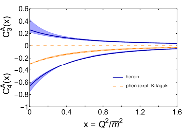
  B

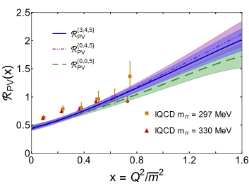
Figure 3: Panel A. Predictions for subdominant transition form factors – blue curves within bracketing uncertainty band: $C^{A}_{4}(x)$, negative curves; and $C^{A}_{3}(x)$, non-negative curves. Both cases: empirical extraction [46, Kitagaki] – dashed orange curve and bracketing band. Panel B. PV ratio, Eq. (10): legend superscript indicates transition form factors retained in the calculation. For comparison, lQCD results [24]: gold squares – $m_{\pi}=297$ MeV, red triangles – $m_{\pi}=330$ MeV.

5. Subdominant $N\to\Delta$ transition form factors —  Our predictions for $C^{A}_{3,4}$ are drawn in Fig. 3A and compared with the phenomenological extractions [46]: the models used therein assume $C^{A}_{3}\equiv 0$ and $C^{A}_{4}=-C^{A}_{5}/4$. Our predictions disagree markedly with those assumptions.

$C^{A}_{3}$ is the weak $N\to\Delta$ analogue of the electric quadrupole ($E2$) form factor in $\gamma N\to\Delta$ transitions [49, 50]. Like the vector $E2$ transition strength, if the nucleon and $\Delta$-baryon are described by SU$(6)$ symmetric (spherical) wave functions, then $C^{A}_{3}\equiv 0$. Evidently, in our Poincaré covariant treatment, $C^{A}_{3}\neq 0$. Indeed, no Poincaré-covariant $N$ or $\Delta$-baryon wave function is simply $\mathsf{S}$-wave in character – see, e.g., the wave functions in Ref. [51]. We find $C^{A}_{3}(x)$ decreases monotonically with increasing $x$ from a maximum value $C^{A}_{3}(0)=0.26^{+0.17}_{-0.04}$.

Considering Fig. 3A, our prediction for $C^{A}_{4}$ exhibits qualitatively similar behaviour to the phenomenological parametrisation. Quantitatively, however, it is uniformly larger in magnitude: we predict $C^{A}_{4}(0)=-0.66^{+0.03}_{-0.10}$, versus $C^{A}_{4}(0)=-0.3$ in the parametrisation.

6. Parity violation asymmetry —  With the construction and use of high-luminosity facilities, spin observables can today be used to probe hadron structure and search for beyond-SM physics – see, e.g., Refs. [52, 53, 54]. One such quantity is the parity-violating asymmetry in electroweak excitation of the $\Delta$-baryon [55]:

$${\mathcal{R}}_{PV}^{\{3,4,5\}}( Q^{2}):=\frac{C^{A}_{5}}{C^{V}_{3}}\bigg{[}1+\frac{m_{\Delta}^{2}-Q^{2}-m_{N}^{2}}{2m_{N}^{2}}\frac{C^{A}_{4}}{C^{A}_{5}}$$

$$-\frac{m_{N}^{2}+Q^{2}+2m_{N}m_{\Delta}-3m_{\Delta}^{2}}{4m_{N}m_{\Delta}}\frac{C^{A}_{3}}{C^{A}_{5}}\bigg{]}\,.$$ (10)

Having calculated the weak $N\to\Delta$ transition form factors, in Fig. 3B we deliver a prediction for this as yet unmeasured ratio. Since $\pi N$ final-state interactions play a material role in understanding the low-$x$ behaviour of $\gamma N\to\Delta$ transition form factors [56] and such effects are difficult to represent reliably – see, e.g., Ref. [31, Sec. 6], we use our predictions for $C_{3,4,5}^{A}$ but construct $C^{V}_{3}$ from the parametrisations presented in Ref. [57, MAID].

Two principal conclusions may be drawn from Fig. 3B: (i) ${\mathcal{R}}_{PV}(0)=0.45(4)>0$, which may be compared with a value of $\approx 0.6$ if one uses the empirical parametrisations from Ref. [46]; and (ii) $C^{A}_{5}$ is dominant on $x\lesssim 0.5$, but $C^{A}_{3,4}$ become increasingly important as $x$ grows.

7. Pseudoscalar transition form factor —  Our prediction for $G_{\pi N\Delta}$ is drawn in Fig. 4. Defined as usual, the $G_{\pi N\Delta}$ radius is $r_{\pi N\Delta}=1.4(1)\,r_{\pi NN}$, where $r_{\pi NN}$ is the $G_{\pi NN}$ analogue [16]. Our prediction is softer than available lQCD results. Notably, owing to a persistent negative contribution from probe seagull couplings to the diquark-quark vertices, we find a zero in $G_{\pi N\Delta}$ at $x=0.84(6)$. (See Fig. 5 and Table 2 in the supplemental material.) Given the large pion masses and poor precision, extant lQCD results cannot test this prediction.

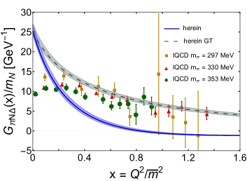
Figure 4: $G_{\pi N\Delta}(x)/m_{N}$ calculated herein – blue curve within uncertainty band; $G^{\prime}_{\pi N\Delta}(x)/m_{N}$ – dashed grey curve and band, where our result for $C^{A}_{5}(x)$ is used on the right in Eq. (12). Comparison: lQCD [23, 24] – hybrid [green circles – $m_{\pi}=353$ MeV] and domain wall fermions [gold squares – $m_{\pi}=297$ MeV, red triangles – $m_{\pi}=330$ MeV]. Our prediction for $G_{\pi N\Delta}(-m_{\pi}^{2})/m_{N}=27.43^{+2.02}_{-0.68}$ is consistent with that obtained using chiral perturbation theory [58].

It is clear from Fig. 4 that the GT relation, Eq. (6), is satisfied: specifically [in $1/$GeV],

$$\frac{G_{\pi N\Delta}(0)}{m_{N}}=25.2^{+1.9}_{-0.7}\;{\rm cf.}\;\frac{2C^{A}_{5}(0)}{f_{\pi}}=25.1^{+1.9}_{-0.6}\,.$$ (11)

As with nucleon and $\Delta$ elastic weak form factors, the GT relation is only valid on $x\simeq 0$. Symmetry guarantees nothing more. We highlight this in Fig. 4 by also plotting

$$G^{\prime}_{\pi N\Delta}(x)/m_{N}:=(2/f_{\pi})C^{A}_{5}(x)\,.$$ (12)

Plainly, $G^{\prime}_{\pi N\Delta}(x)\approx G_{\pi N\Delta}(x)$ only on $x\lesssim 0.1$. (Additional remarks on PCAC are contained in the supplemental material.)

8. Summary —  Using a Poincaré-covariant, symmetry-preserving treatment of the continuum baryon bound-state problem, in which all elements possess an unambiguous link with analogous quantities in QCD, we delivered parameter-free predictions for every form factor associated with $N\to\Delta$ transitions driven by axial or pseudoscalar probes. In doing so, we completed a unified description of, inter alia, all $N$ and/or $\Delta$-baryon axialvector and pseudoscalar currents. Where comparisons with data are available, our predictions are confirmed. Hence, the results herein can serve as a reliable resource for use in analysing existing and anticipated data relevant to worldwide efforts focused on elucidation of $\nu$, $\bar{\nu}$ properties. No material improvement upon our results may be envisaged before the same array of observables can be calculated using either the explicit three-body Poincaré-covariant Faddeev equation approach to $N$, $\Delta$ elastic and transition form factors or numerical simulations of lQCD.

Acknowledgments — We are grateful for constructive communications with K. Graczyk, T.-S. H. Lee, A. Lovato and T. Sato. Work supported by: National Natural Science Foundation of China (grant nos. 12135007, 12247103); and Deutsche Forschungsgemeinschaft (grant no. FI 970/11-1).

Supplemental Material

This material is included with a view to illustrating/exemplifying remarks in the main text, including, in some cases, numerical confirmation of observations inferred from figures, and supplying practicable representations of the form factor predictions.

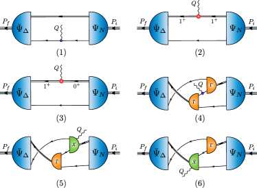
Figure 5: Symmetry-preserving axial/pseudoscalar current for on-shell baryons ($B=N,\Delta$) that are described by the Faddeev amplitudes $\Psi_{B}$ obtained by solving the equation depicted in Fig. 1. Single line – dressed-quark propagator; undulating line – axial/pseudoscalar current; $\Gamma$ – diquark correlation amplitude; double line – diquark propagator; and $\chi$ – seagull terms.

Within the quark + diquark picture of baryons, the axial and pseudoscalar currents, Eqs. (1b) and (4), can both be decomposed into a sum of six terms, depicted in Fig. 5. Evidently, the probe interacts with the dressed-quarks and -diquarks in various ways, each of which is detailed in Ref. [16, Sec. IIIC]. Referring to Fig. 5, in Table 2 we list the relative strength of each diagram’s contribution to $C^{A}_{3,4,5,6}(0)$ and $G_{\pi N\Delta}(0)$.

Table 2: Referring to Fig. 5, separation of the axial-vector form factors $C^{A}_{i}(0)$ $(i=3,4,5,6)$, and the $\pi N\Delta$ form factor $G_{\pi N\Delta}(0)$ into contributions from various diagrams, listed as a fraction of the total $Q^{2}=0$ value. Diagram (1): $\langle J\rangle^{A}_{\rm q}$ – weak- or pseudoscalar-probe strikes dressed-quark with axialvector diquark spectator. Diagram (2): $\langle J\rangle^{AA}_{\rm qq}$ – probe strikes axialvector diquark with dressed-quark spectator. Diagram (3): $\langle J\rangle^{AS}_{\rm qq}$ – probe mediates scalar to axialvector diquark transition, with dressed-quark spectator. Diagram (4): $\langle J\rangle_{\rm ex}$ – probe strikes dressed-quark “in-flight” between one diquark correlation and another. Diagrams (5) and (6): $\langle J\rangle_{\rm sg}$ – probe couples inside the diquark correlation amplitude. The listed uncertainties reflect the impact of $\pm 5$% variations in the diquark masses in Eq. (7), e.g., $-0.11_{6_{\mp}}\Rightarrow-0.11\mp 0.06$.

	$\ \langle J\rangle^{A}_{\rm q}$	$\langle J\rangle^{AA}_{\rm qq}$	$\langle J\rangle^{AS}_{\rm qq}$	$\langle J\rangle_{\rm ex}$	$\ \langle J\rangle_{\rm sg}$
$C^{A}_{5}(0)\$	$\phantom{-}0.48_{9_{\pm}}$	$0.017_{5_{\pm}}$	$0.21_{1_{\pm}}$	$0.29_{10_{\mp}}$	$\phantom{-}0$
$C^{A}_{6}(0)\$	$\phantom{-}0.50_{9_{\pm}}$	$0.016_{5_{\pm}}$	$0.21_{1_{\pm}}$	$0.52_{8_{\mp}}$	$-0.25_{2_{\mp}}$
$C^{A}_{3}(0)\$	$-0.11_{5_{\pm}}$	$0.14_{12_{\pm}}$	$0.37_{10_{\pm}}$	$0.60_{27_{\mp}}$	$\phantom{-}0$
$C^{A}_{4}(0)\$	$\phantom{-}0.44_{8_{\pm}}$	$0.052_{37_{\pm}}$	$0.23_{2_{\pm}}$	$0.28_{10_{\mp}}$	$\phantom{-}0$
$G_{\pi N\Delta}(0)\$	$\phantom{-}0.53_{11_{\pm}}$	$0.020_{4_{\pm}}$	$0.17_{2_{\pm}}$	$0.57_{10_{\mp}}$	$-0.29_{3_{\mp}}$

In order to assist others in employing our predictions for the form factors associated with nucleon–to–$\Delta$ axial and pseudoscalar transition currents, here we present practicable parametrisations, valid as interpolations and useful for extrapolation. We considered a range of options, achieving good results with the following functional forms:

$${\mathscr{F}}(x)=\frac{n^{0}_{\mathscr{F}}+n^{1}_{\mathscr{F}}x/(n^{2}_{\mathscr{F}}+x)^{2}}{(1+d^{1}_{\mathscr{F}}x)^{2}}\,,$$ (13)

for ${\mathscr{F}}=C^{A}_{i=3,4,5}$;

$$C^{A}_{6}(x)=\frac{n^{0}_{C^{A}_{6}}+n^{1}_{C^{A}_{6}}x/(n^{2}_{C^{A}_{6}}+x)^{2}}{(1+d^{1}_{C^{A}_{6}}x)^{2}}\frac{\mu_{N}}{x+\mu_{\pi}}\,,$$ (14)

reflecting PPD, Eq. (9); and

$$G_{\pi N\Delta}/m_{N}=\frac{n^{0}_{G}+n^{1}_{G}x}{1+d^{1}_{G}x+d^{2}_{G}x^{2}+d^{3}_{G}x^{3}}\,.$$ (15)

All interpolation coefficients are listed in Table 3.

Table 3: Interpolation parameters for the $N\to\Delta$ axial and pseudoscalar transition form factors, for use in Eqs. (15), (14). All dimensionless, except $n^{0,1}_{G}$, the numerator coefficients for $G_{\pi\Delta\Delta}/m_{N}$ in Eq. (15), which are listed in GeV^-1.

	$C^{A}_{5}$	$C^{A}_{6}$	$C^{A}_{3}$	$C^{A}_{4}$	$G_{\pi N\Delta}/m_{N}$
$n^{0}\$	$\phantom{-}1.16^{+0.09}_{-0.03}$	$\phantom{-}1.43^{+0.17}_{-0.10}$	$\phantom{-}0.26^{+0.17}_{-0.04}$	$-0.66^{+0.03}_{-0.10}$	$\phantom{-}25.15^{+1.90}_{-0.67}$
$n^{1}\$	$-0.27^{-0.19}_{+0.07}$	$-0.22^{-0.13}_{+0.03}$	$-0.87^{+0.34}_{+0.35}$	$\phantom{-}7.85^{-1.22}_{-0.84}$	$-30.29^{+0.34}_{-1.27}$
$n^{2}\$	$\phantom{-}0.46^{+0.05}_{-0.07}$	$\phantom{-}0.17^{+0.02}_{+0.03}$	$\phantom{-}2.02^{-1.25}_{+0.68}$	$\phantom{-}3.67^{-0.35}_{-0.46}$
$d^{1}\$	$\phantom{-}0.87^{-0.06}_{+0.06}$	$\phantom{-}1.06^{-0.01}_{+0.01}$	$\phantom{-}0.62^{+0.33}_{+0.17}$	$\phantom{-}0.70^{-0.12}_{+0.24}$	$\phantom{-}3.31^{+0.01}_{+0.15}$
$d^{2}\$					$\phantom{-}2.53^{+0.22}_{+0.15}$
$d^{3}\$					$\phantom{-}1.88^{-0.58}_{+0.36}$

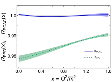
Figure 6: Quantitative verification of the accuracy of the PPD approximation – Eq. (16): dashed green curve within lighter band; and numerical verification of the PCAC relation – Eq. (17): solid blue curve within lighter band.

The off-diagonal PPD approximation is written in Eq. (9). Here we choose to supplement Fig. 2 with additional quantitative information. Consider, therefore, the following ratio

$$R_{PPD}:=\frac{\mu_{N}C^{A}_{5}}{(x+\mu_{\pi})C^{A}_{6}}\,.$$ (16)

The calculated result is depicted in Fig. 6. The $x$-dependence of $R_{PPD}$ is very much like the analogous curves obtained for the nucleon [16, Fig. 8] and the $\Delta(1232)$-baryon [29, Fig. 8]: it lies $<2.5\%$ below unity on $x\simeq 0$ and grows toward unity as $x$ increases. The explanation for the accuracy and behaviour of this approximating formula can be found, e.g., in Ref. [29, Sec. 4.3].

Some corollaries of PCAC were discussed in connection with Eqs. (11), (12). As done separately for the nucleon and $\Delta$-baryon weak elastic form factors [16, 29], they may be extended. Indeed, following Ref. [29, Sec. 4.3], one can prove algebraically that $C^{A}_{5}$, $C^{A}_{6}$, and $G_{\pi N\Delta}$ satisfy the off-diagonal PCAC relation, Eq. (5), as they must in any symmetry preserving treatment of $N\to\Delta$ weak transitions. Thus, the PCAC ratio

$$R_{PCAC}:=\frac{2m_{N}\mu_{N}C^{A}_{5}}{2m_{N}xC^{A}_{6}+\mu_{N}\mu_{\pi}f_{\pi}G_{\pi N\Delta}/(x+\mu_{\pi})}\,,$$ (17)

should be unity. We draw the numerical result for this ratio in Fig. 6: evidently, allowing for numerical accuracy, the curve is indistinguishable from unity. The uncertainty band highlights that the result is parameter-independent.

References

- Fukuda et al. [1998] Y. Fukuda, et al., Evidence for oscillation of atmospheric neutrinos, Phys. Rev. Lett. 81 (1998) 1562–1567.
- Kajita [2016] T. Kajita, Nobel Lecture: Discovery of atmospheric neutrino oscillations, Rev. Mod. Phys. 88 (2016) 030501.
- McDonald [2016] A. B. McDonald, Nobel Lecture: The Sudbury Neutrino Observatory: Observation of flavor change for solar neutrinos, Rev. Mod. Phys. 88 (2016) 030502.
- Alvarez-Ruso et al. [2018] L. Alvarez-Ruso, et al., NuSTEC White Paper: Status and challenges of neutrino–nucleus scattering, Prog. Part. Nucl. Phys. 100 (2018) 1–68.
- Argüelles et al. [2020] C. A. Argüelles, et al., New opportunities at the next-generation neutrino experiments I: BSM neutrino physics and dark matter, Rept. Prog. Phys. 83 (12) (2020) 124201.
- Abi et al. [2020] B. Abi, et al., Long-baseline neutrino oscillation physics potential of the DUNE experiment, Eur. Phys. J. C 80 (10) (2020) 978.
- Formaggio et al. [2021] J. A. Formaggio, A. L. C. de Gouvêa, R. G. H. Robertson, Direct Measurements of Neutrino Mass, Phys. Rept. 914 (2021) 1–54.
- Abusleme et al. [2022] A. Abusleme, et al., JUNO physics and detector, Prog. Part. Nucl. Phys. 123 (2022) 103927.
- Lokhov et al. [2022] A. Lokhov, S. Mertens, D. S. Parno, M. Schlösser, K. Valerius, Probing the Neutrino-Mass Scale with the KATRIN Experiment, Ann. Rev. Nucl. Part. Sci. 72 (2022) 259–282.
- Ruso et al. [2022] L. A. Ruso, et al., Theoretical tools for neutrino scattering: interplay between lattice QCD, EFTs, nuclear physics, phenomenology, and neutrino event generators – arXiv:2203.09030 [hep-ph] .
- Sajjad Athar et al. [2023] M. Sajjad Athar, A. Fatima, S. K. Singh, Neutrinos and their interactions with matter, Prog. Part. Nucl. Phys. 129 (2023) 104019.
- Mosel [2016] U. Mosel, Neutrino Interactions with Nucleons and Nuclei: Importance for Long-Baseline Experiments, Ann. Rev. Nucl. Part. Sci. 66 (2016) 171–195.
- Hill et al. [2018] R. J. Hill, P. Kammel, W. J. Marciano, A. Sirlin, Nucleon Axial Radius and Muonic Hydrogen — A New Analysis and Review, Rept. Prog. Phys. 81 (2018) 096301.
- Gysbers et al. [2019] P. Gysbers, et al., Discrepancy between experimental and theoretical -decay rates resolved from first principles, Nature Phys. 15 (5) (2019) 428–431.
- Lovato et al. [2020] A. Lovato, J. Carlson, S. Gandolfi, N. Rocco, R. Schiavilla, Ab initio study of and inclusive scattering in 12C: confronting the MiniBooNE and T2K CCQE data, Phys. Rev. X 10 (2020) 031068.
- Chen et al. [2022] C. Chen, C. S. Fischer, C. D. Roberts, J. Segovia, Nucleon axial-vector and pseudoscalar form factors and PCAC relations, Phys. Rev. D 105 (9) (2022) 094022.
- Chen and Roberts [2022] C. Chen, C. D. Roberts, Nucleon axial form factor at large momentum transfers, Eur. Phys. J. A 58 (2022) 206.
- Alexandrou et al. [2017] C. Alexandrou, M. Constantinou, K. Hadjiyiannakou, K. Jansen, C. Kallidonis, G. Koutsou, A. Vaquero Aviles-Casco, Nucleon axial form factors using = 2 twisted mass fermions with a physical value of the pion mass, Phys. Rev. D 96 (2017) 054507.
- Jang et al. [2020] Y.-C. Jang, R. Gupta, B. Yoon, T. Bhattacharya, Axial Vector Form Factors from Lattice QCD that Satisfy the PCAC Relation, Phys. Rev. Lett. 124 (2020) 072002.
- Bali et al. [2020] G. S. Bali, L. Barca, S. Collins, M. Gruber, M. Löffler, A. Schäfer, W. Söldner, P. Wein, S. Weishäupl, T. Wurm, Nucleon axial structure from lattice QCD, JHEP 05 (2020) 126 (2020).
- Sato et al. [2003] T. Sato, D. Uno, T. S. H. Lee, Dynamical model of weak pion production reactions, Phys. Rev. C 67 (2003) 065201.
- Simons et al. [2022] D. Simons, N. Steinberg, A. Lovato, Y. Meurice, N. Rocco, M. Wagman, Form factor and model dependence in neutrino-nucleus cross section predictions – arXiv:2210.02455 [hep-ph] .
- Alexandrou et al. [2007] C. Alexandrou, G. Koutsou, T. Leontiou, J. W. Negele, A. Tsapalis, Axial Nucleon and Nucleon to Delta form factors and the Goldberger-Treiman Relations from Lattice QCD, Phys. Rev. D 76 (2007) 094511, [Erratum: Phys. Rev. D 80, 099901 (2009)].
- Alexandrou et al. [2011] C. Alexandrou, G. Koutsou, J. W. Negele, Y. Proestos, A. Tsapalis, Nucleon to Delta transition form factors with domain wall fermions, Phys. Rev. D 83 (2011) 014501.
- Eichmann et al. [2016] G. Eichmann, H. Sanchis-Alepuz, R. Williams, R. Alkofer, C. S. Fischer, Baryons as relativistic three-quark bound states, Prog. Part. Nucl. Phys. 91 (2016) 1–100.
- Barabanov et al. [2021] M. Y. Barabanov, et al., Diquark Correlations in Hadron Physics: Origin, Impact and Evidence, Prog. Part. Nucl. Phys. 116 (2021) 103835.
- Ding et al. [2023] M. Ding, C. D. Roberts, S. M. Schmidt, Emergence of Hadron Mass and Structure, Particles 6 (1) (2023) 57–120.
- Carman et al. [2023] D. S. Carman, R. W. Gothe, V. I. Mokeev, C. D. Roberts, Nucleon Resonance Electroexcitation Amplitudes and Emergent Hadron Mass, Particles 6 (1) (2023) 416–439.
- Yin et al. [2023] P.-L. Yin, C. Chen, C. S. Fischer, C. D. Roberts, -Baryon axialvector and pseudoscalar form factors, and associated PCAC relations, Eur. Phys. J. A 59 (7) (2023) 163.
- Itzykson and Zuber [1980] C. Itzykson, J.-B. Zuber, Quantum Field Theory, McGraw-Hill Inc., New York, 1980.
- Segovia et al. [2014] J. Segovia, I. C. Cloet, C. D. Roberts, S. M. Schmidt, Nucleon and elastic and transition form factors, Few Body Syst. 55 (2014) 1185–1222.
- Adler [1968] S. L. Adler, Photoproduction, electroproduction and weak single pion production in the (3,3) resonance region, Annals Phys. 50 (1968) 189–311.
- Llewellyn Smith [1972] C. H. Llewellyn Smith, Neutrino Reactions at Accelerator Energies, Phys. Rept. 3 (1972) 261–379.
- Workman et al. [2022] R. L. Workman, et al., Review of Particle Physics, PTEP 2022 (2022) 083C01.
- Cui et al. [2020] Z.-F. Cui, J.-L. Zhang, D. Binosi, F. de Soto, C. Mezrag, J. Papavassiliou, C. D. Roberts, J. Rodríguez-Quintero, J. Segovia, S. Zafeiropoulos, Effective charge from lattice QCD, Chin. Phys. C 44 (2020) 083102.
- Deur et al. [2024] A. Deur, S. J. Brodsky, C. D. Roberts, QCD Running Couplings and Effective Charges, Prog. Part. Nucl. Phys. 134 (2024) 104081.
- Cahill et al. [1989] R. T. Cahill, C. D. Roberts, J. Praschifka, Baryon structure and QCD, Austral. J. Phys. 42 (1989) 129–145.
- Reinhardt [1990] H. Reinhardt, Hadronization of Quark Flavor Dynamics, Phys. Lett. B 244 (1990) 316–326.
- Efimov et al. [1990] G. V. Efimov, M. A. Ivanov, V. E. Lyubovitskij, Quark - diquark approximation of the three quark structure of baryons in the quark confinement model, Z. Phys. C 47 (1990) 583–594.
- Roberts et al. [2021] C. D. Roberts, D. G. Richards, T. Horn, L. Chang, Insights into the emergence of mass from studies of pion and kaon structure, Prog. Part. Nucl. Phys. 120 (2021) 103883.
- Binosi [2022] D. Binosi, Emergent Hadron Mass in Strong Dynamics, Few Body Syst. 63 (2) (2022) 42.
- Salmè [2022] G. Salmè, Explaining mass and spin in the visible matter: the next challenge, J. Phys. Conf. Ser. 2340 (1) (2022) 012011.
- de Teramond [2022] G. F. de Teramond, Emergent phenomena in QCD: The holographic perspective – arXiv:2212.14028 [hep-ph], in: 25th Workshop on What Comes Beyond the Standard Models?, 2022.
- Ferreira and Papavassiliou [2023] M. N. Ferreira, J. Papavassiliou, Gauge Sector Dynamics in QCD, Particles 6 (1) (2023) 312–363.
- Krein [2023] G. Krein, Femtoscopy of the Matter Distribution in the Proton, Few Body Syst. 64 (3) (2023) 42.
- Kitagaki et al. [1990] T. Kitagaki, et al., Study of and using the BNL 7-foot deuterium filled bubble chamber, Phys. Rev. D 42 (1990) 1331–1338.
- Schreiner and Von Hippel [1973] P. A. Schreiner, F. Von Hippel, Neutrino production of the Delta (1236), Nucl. Phys. B 58 (1973) 333–362.
- Meyer et al. [2016] A. S. Meyer, M. Betancourt, R. Gran, R. J. Hill, Deuterium target data for precision neutrino-nucleus cross sections, Phys. Rev. D 93 (2016) 113015.
- Liu et al. [1995] J. Liu, N. C. Mukhopadhyay, L.-s. Zhang, Nucleon to delta weak excitation amplitudes in the nonrelativistic quark model, Phys. Rev. C 52 (1995) 1630–1647.
- Barquilla-Cano et al. [2007] D. Barquilla-Cano, A. J. Buchmann, E. Hernandez, Axial and transition form factors, Phys. Rev. C 75 (2007) 065203, [Erratum: Phys.Rev.C 77, 019903 (2008)].
- Liu et al. [2022] L. Liu, C. Chen, Y. Lu, C. D. Roberts, J. Segovia, Composition of low-lying -baryons, Phys. Rev. D 105 (11) (2022) 114047.
- Androic et al. [2011] D. Androic, et al., The G0 Experiment: Apparatus for Parity-Violating Electron Scattering Measurements at Forward and Backward Angles, Nucl. Instrum. Meth. A 646 (2011) 59–86.
- Becker et al. [2018] D. Becker, et al., The P2 experiment, Eur. Phys. J. A 54 (11) (2018) 208.
- Arrington et al. [2023] J. Arrington, et al., The solenoidal large intensity device (SoLID) for JLab 12 GeV, J. Phys. G 50 (11) (2023) 110501.
- Mukhopadhyay et al. [1998] N. C. Mukhopadhyay, M. J. Ramsey-Musolf, S. J. Pollock, J. Liu, H. W. Hammer, Parity violating excitation of the Delta (1232): Hadron structure and new physics, Nucl. Phys. A 633 (1998) 481–518.
- Julia-Diaz et al. [2007] B. Julia-Diaz, T. S. H. Lee, T. Sato, L. C. Smith, Extraction and Interpretation of Form Factors within a Dynamical Model, Phys. Rev. C 75 (2007) 015205.
- Drechsel et al. [2007] D. Drechsel, S. S. Kamalov, L. Tiator, Unitary Isobar Model - MAID2007, Eur. Phys. J. A 34 (2007) 69–97.
- Ünal et al. [2021] Y. Ünal, A. Küçükarslan, S. Scherer, Axial-vector nucleon-to-delta transition form factors using the complex-mass renormalization scheme, Phys. Rev. D 104 (9) (2021) 094014.