Measurements of higher-order cumulants of multiplicity and net-electric charge distributions in inelastic proton-proton interactions by CERN-EP-2023-290 This paper presents the energy dependence of multiplicity and net-electric charge fluctuations in interactions at beam momenta 20, 31, 40, 80, and 158 . Results are corrected for the experimental biases and quantified with the use of cumulants and factorial cumulants. Data are compared with the and FTFP-BERT model predictions.

1 Introduction

This paper presents experimental results on event-by-event fluctuations of multiplicities of all charged, positively, and negatively charged hadrons as well as fluctuations of net-electric charge (so-called net-charge) produced in inelastic proton-proton () interactions at beam momenta 20, 31, 40, 80, and 158 . The corresponding energy per nucleon pair in the center-of-mass system is 6.3, 7.7, 8.8, 12.3, and 17.3 GeV, respectively.

The measurements were performed by the multi-purpose  [1] spectrometer at the CERN Super Proton Synchrotron (SPS) in 2009. They are part of the strong interactions program devoted to studying the properties of the onset of deconfinement and searching for the critical point (CP) of the strongly interacting matter [2].

Fluctuation and correlation analyses may be sensitive to CP [3, 4] due to their connection with correlation length. Other effects may dilute the CP signal, e.g., local and global conservation laws [5]. Thus, establishing the baseline signal is a complex and demanding task. Results on interactions give a unique opportunity to test models of strong interactions which help to understand results on nucleus-nucleus collisions. Rich experimental data in interactions on particle production in full-phase space is already available from bubble-chamber or streamer experiments [6]. It should be underlined that the data statistics of these experiments are considerably smaller than nowadays measurements (see Sec. 4). In case of fluctuations, those measurements and predictions (like KNO-G scaling [7, 8, 9]) are difficult to compare to modern experimental analysis due to different analysis acceptance [10].

Throughout this paper, the rapidity: $y=0.5\ln[(E+cp_{\text{L}})/(E-cp_{\text{L}})]$, is calculated in the collision center-of-mass system by shifting rapidity in the laboratory frame by rapidity of the center-of-mass, assuming proton mass. The $E$, $p_{\text{L}}$, and $c$ are the particle energy (assuming pion mass for a given charged particle), its longitudinal momentum, and the velocity of light, respectively. The transverse component of the momentum is denoted as $p_{\text{T}}$, and the azimuthal angle $\phi$ is the angle between the transverse momentum vector and the horizontal (x) axis. Total momentum in the laboratory system is denoted as $p$. The collision energy per nucleon pair in the center-of-mass system is denoted as $\sqrt{s_{\emph{NN}}}$.

2 Intensive quantities

Net-charge, as well as multiplicity fluctuations, are one of the tools to search for CP in nucleus-nucleus collisions. Although there is great freedom in selecting fluctuation measures, it is reasonable to choose ones sensitive to the desired physical phenomenon and insensitive to other possible sources of fluctuations, e.g., system volume ($V$). As interactions are measured as a reference for nucleus-nucleus collisions, choosing quantities that make comparing systems easier is particularly important.

It is more convenient to present results in terms of cumulants than moments of the multiplicity distribution [11]. Cumulants and moments are proportional to $V$ and called extensive variables ($\sim V$) [11]. If the event quantity $N$ is measured, then the $n$-th order moment of its probability distribution, $P(N)$, is defined by

$$\langle N^{n}\rangle=\sum_{N}N^{n}P(N),$$ (1)

where $\langle\dots\rangle$ denotes averaging over events. Then, the first four cumulants are given by

$$\kappa_{1}[N]=\langle N\rangle,$$ (2)

$$\kappa_{2}[N]=\langle\delta N^{2}\rangle,$$ (3)

$$\kappa_{3}[N]=\langle\delta N^{3}\rangle,$$ (4)

$$\kappa_{4}[N]=\langle\delta N^{4}\rangle-3\langle\delta N^{2}\rangle^{2},$$ (5)

where $\langle\delta N^{n}\rangle=\langle(N-\langle N\rangle)^{n}\rangle$.

A ratio of two extensive quantities is an intensive quantity, e.g., the scaled variance of $N$:

$$\omega[N]=\frac{\kappa_{2}[N]}{\kappa_{1}[N]}.$$ (6)

The scaled variance calculated within a simple model like the ideal Boltzmann gas described in the Grand Canonical Ensemble (GCE) reads [12]:

$$\omega[N]=\omega[N]^{*}+\langle N\rangle/\langle V\rangle\cdot\omega[V],\\$$ (7)

where $\omega[N]^{*}$ stands for the scaled variance at fixed volume $V$. The first component $\omega[N]^{*}$ of Eq. 7 is considered the wanted one, and it is independent of the volume fluctuations. However, the second component is seen as unwanted as it is trivially proportional to the scaled variance of the volume distribution $\omega[V]$.

In GCE, intensive quantity $\omega$ has the following features:

1. it is independent of $V$ (for event ensembles with fixed $V$),

2. it depends on fluctuations of $V$ (even if $\langle V\rangle$ is fixed),

3. for Poisson distribution it is equal to unity.

For third and fourth-order cumulants, one can construct intensive quantities similarly as:

$$\frac{\kappa_{3}[N]}{\kappa_{2}[N]},\quad\frac{\kappa_{4}[N]}{\kappa_{2}[N]}.$$ (8)

These quantities also are intensive so independent of volume but they remain sensitive to the $V$ fluctuations [13, 12, 14].

The Poisson distribution is considered the reference as particles produced in GCE will follow it with the $\lambda$ parameter being equal to the average multiplicity of a given particle type [15, 16]. The sum of charges in the ideal gas model also will follow the Poisson distribution. In the ideal gas model, the net-charge distribution will be the Skellam distribution, which is defined as a difference between two Poisson distributions of positively and negatively charged particles with constants $\langle h^{+}\rangle$ and $\langle h^{-}\rangle$, where $h^{+}$ and $h^{-}$ stand for multiplicities of positively and negatively charged hadrons. The following relation gives the Skellam distribution cumulants: $\kappa_{i}=\langle h^{+}\rangle+(-1)^{i}\langle h^{-}\rangle$, where $i$ is the cumulant order. In such a case, ratios of even and odd cumulants will not keep one as a reference value. The modification of the reference for net-charge, so it remains one and is intensive can be introduced in the following way:

$$\frac{\kappa_{2}[h^{+}-h^{-}]}{\kappa_{1}[h^{+}]+\kappa_{1}[h^{-}]},\quad\frac{\kappa_{3}[h^{+}-h^{-}]}{\kappa_{1}[h^{+}-h^{-}]}.$$ (9)

The use of intensive quantities is crucial in the case of comparisons between and nucleus-nucleus collisions. Cumulants mix information about correlations of different orders; for details of the relation see Ref. [17]. Factorial cumulants are constructed to cancel all lower-order correlations so only a given order of correlations can be studied [17, 18, 19]. They do not keep one as a reference and are defined as:

$$\hat{C}_{2}[N]= -\kappa_{1}[N]+\kappa_{2}[N],$$ (10)

$$\hat{C}_{3}[N]= 2\kappa_{1}[N]-3\kappa_{2}[N]+\kappa_{3}[N],$$ (11)

$$\hat{C}_{4}[N]= -6\kappa_{1}[N]+11\kappa_{2}[N]-6\kappa_{3}[N]+\kappa_{4}[N].$$ (12)

3 Experimental setup

The experiment [1] is a large acceptance hadron spectrometer located in the H2 beam line of the CERN North Area. The schematic layout of the detector components is shown in Fig. 1.

The results presented in this paper were obtained using measurements from the Time Projection Chambers (TPC), the Beam Position Detectors (BPD), and the beam and trigger counters. As many publications concerning are available, we provide only a brief description of the detector system. The detector elements, the proton beam, the liquid hydrogen target, and the data reconstruction procedure are described in detail in Refs. [1, 20, 21].

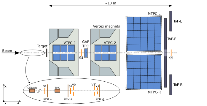
Figure 1: (Color online) The schematic layout of the experiment during data taking in 2009 at the CERN SPS (horizontal cut, not to scale), see text and Ref. [1] for details.

For data taking on interactions, a liquid hydrogen target of 20.29 cm length (2.8% interaction length) and 3 cm diameter was placed 88.4 cm upstream of VTPC-1.

Secondary beams of positively charged hadrons at 20, 31, 40, 80, and 158 were produced from 400 protons extracted from the SPS onto a beryllium target. Protons from the secondary hadron beam were identified by two Cherenkov counters, a CEDAR (either CEDAR-W or CEDAR-N) and a threshold counter (THC). Due to their limited range of operation, two different CEDAR counters were employed, namely for beams at 31, and 40 the CEDAR-W counter and for beams at 80 and 158 the CEDAR-N counter. The threshold counter was used for all beam energies. A selection based on signals from the Cherenkov counters allowed the identification of beam protons with a purity of about 99%. A coincidence of these signals provided the beam trigger $T_{\text{beam}}$.

A set of scintillation, Cherenkov counters, and beam position detectors (BPDs) upstream of the spectrometer provide timing reference, identification, and position measurements of incoming beam particles. Trajectories of individual beam particles were measured in a telescope of beam position detectors placed along the beamline (BPD-1/2/3 in Fig. 1).

Two scintillation counters, S1 and S2, provided beam definition, together with the three veto counters V0, V1 and V1^p with a 1 cm diameter hole. The S1 counter also provided the timing (start time for the gating of all counters). Beam protons were then selected by the coincidence:

$$T_{\text{beam}}=\textrm{S1}\wedge\textrm{S2}\wedge\overline{\textrm{V0}}\wedge\overline{\textrm{V1}}\wedge\overline{\textrm{V1}^{\mathrm{p}}}\wedge\textrm{CEDAR}\wedge\overline{\textrm{THC}}\leavevmode\nobreak\ .$$ (13)

The interaction trigger $T_{\text{int}}$ was provided by the anti-coincidence of the incoming hadron beam and a scintillation counter S4 ($T_{\text{int}}=T_{\text{beam}}\wedge\overline{\textrm{S4}}$). The S4 counter, with a two-centimeter diameter, was placed between the VTPC-1 and VTPC-2 detectors along the beam trajectory at about 3.7 m from the target, see Fig. 1.

The main tracking devices of the spectrometer are four large volume TPCs. Two of them, the vertex TPCs (VTPC-1 and VTPC-2), are located in the magnetic fields of two super-conducting dipole magnets with a maximum combined bending power of 9 Tm, which corresponds to about 1.5 T and 1.1 T fields in the upstream and downstream magnets, respectively. To optimize the acceptance of the detector, the fields in both magnets were set in proportion to the beam momentum. Two large main TPCs (MTPC-L and MTPC-R) are positioned downstream of the magnets symmetrically to the beam line. The fifth small TPC (GAP TPC) is placed between VTPC-1 and VTPC-2 directly on the beam line. The TPCs are filled with Ar:CO₂ gas mixtures in proportion 90:10 for the VTPCs and the GAP TPC, and 95:5 for the MTPCs. The TPCs provide measurements of energy loss ${\text{d}}E\!/\!{\text{d}}x$ of charged particles in the chamber gas along their trajectories. Simultaneous measurements of ${\text{d}}E\!/\!{\text{d}}x$ and $p$ allow extracting information on particle mass, which is used to identify charged particles. In the case of this analysis, ${\text{d}}E\!/\!{\text{d}}x$ is used only for electron contamination removal.

4 Analysis

This section starts with a brief overview of the data analysis procedure and the applied corrections. It also defines which class of particles the final results correspond to.

The final results refer to charged hadrons produced in inelastic interactions by strong interaction processes and electromagnetic decays of produced hadrons. Such hadrons are referred to as primary hadrons obtained within the analysis acceptance [22] (for details, see Sec.4.1). Considered charge combinations are indicated as:

1. $h^{+}+h^{-}$ – all charged hadrons,

2. $h^{+}$ – positively charged hadrons,

3. $h^{-}$ – negatively charged hadrons,

4. $h^{+}-h^{-}$ – net-charge being defined as the difference between positively and negatively charged hadrons in a given event.

The availability of the whole distributions and their cumulants $\kappa_{i}$ should allow the reader to obtain the desired quantity if it is not provided here.

The analysis procedure consists of the following steps:

1. application of event and track selection criteria,

2. determination of all charged, positively, and negatively charged hadron multiplicity distributions as well as the net-charge distributions,

3. evaluation of corrections to the distributions based on experimental data and simulations,

4. calculation of the corrected moments and fluctuation quantities,

5. calculation of statistical and estimation of systematic uncertainties.

Corrections for the following biases were evaluated and applied:

1. contribution of particles other than primary hadrons produced in inelastic interactions,

2. losses of primary hadrons due to measurement inefficiencies,

3. losses of inelastic interactions due to the trigger and the event and track selection criteria employed in the analysis.

The corrections are calculated using the unfolding procedure [23] performed on the distributions of the given charge combination after the event and track selection. The analysis acceptance was taken from Ar+Sc analysis [22] (see Sec. 4.1).

4.1 Analysis acceptance

Fluctuation results can not be corrected for limited analysis acceptance. In Ref. [24], fluctuations of multiplicity and transverse momentum up to second-order moments were analyzed in the entire high-quality phase-space region of the NA61/SHINE detector available for interactions at a given beam momenta [25]. As the results of this analysis are planned to be compared to analysis results in nucleus-nucleus collisions, a different acceptance of the high-quality phase-space region of the NA61/SHINE detector in Ar+Sc interactions was used [22]. Among others cut on upper $p_{\text{T}}<1.5$ and rapidity of the track assuming pion mass $0<y_{\pi}<y_{\text{beam}}$, where $y_{\text{beam}}$ is the rapidity of the beam are included in Ar+Sc acceptance maps. The Figure 2 presents both acceptances in interactions at 158 .

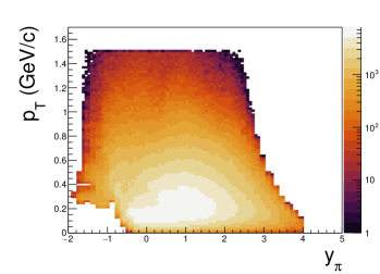
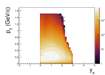
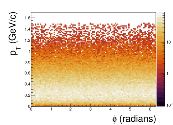
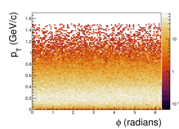
Figure 2: Analysis acceptances in $y_{\pi}-p_{\text{T}}$ and $\phi-p_{\text{T}}$ of charged hadrons in interactions at 158 used in Ref. [24] (left) and analysis acceptance in interactions at 158 common with nucleus-nucleus analysis [22] (right).

Following Ref. [10] we calculate a fraction of accepted particles $x^{i}$ using the  [26, 27] model as:

$$x^{i}=\frac{h_{acc}^{i}}{h^{i}},$$ (14)

where $i$ stands for considered charge combination, $h_{acc}^{i}$ indicates the number of $i$-th particles in the analysis acceptance, and $h^{i}$ is the total number of $i$-th particles. The $x^{i}$ values for interactions in are given in Tab. 1.

$\sqrt{s_{NN}}$ (GeV)	$h^{+}$	$h^{-}$	$h^{+}+h^{-}$	$h^{+}-h^{-}$
6.3	0.24	0.26	0.25	0.23
7.7	0.25	0.28	0.26	0.23
8.8	0.26	0.30	0.27	0.23
12.3	0.30	0.36	0.32	0.24
17.3	0.35	0.43	0.38	0.26

Table 1: Fraction of the accepted charged hadrons and net-charge in interactions within the analysis acceptance [22] based on the model.

4.2 Event and track selection

Analyzed data consists only of events passing the trigger (Trigger in Tab. 2) condition. In the selected events, the trajectory of the beam particle was measured in at least one of BPD-1 or BPD-2 and in the BPD-3 detector (BPD in Tab. 2). To avoid bias from off-time events, an event is accepted only if it does not have the off-time beam particle within $\pm 1$ $\mu$s around the trigger (beam) particle (WFA beam in Tab. 2). The main vertex z-coordinate of the event has to be between $\pm 20$ cm around the center of the liquid hydrogen target (fitted vertex z position in Tab. 2). A small fraction of elastic events that pass the trigger condition (for beam momenta below 158 ) is removed by the removal of events with a single positive track with momentum close to beam momentum ($p\approx p_{\text{beam}}$ in Tab. 2). For details, see Ref. [21]. A summary of the event selection (called standard cuts) is given in the upper part of Table 2. The final number of events selected for the analysis is provided in Table 3.

	standard cuts	loose cuts	tight cuts
Trigger	applied
BPD	applied
WFA beam	$<\pm 1\leavevmode\nobreak\ \mu$s	no cut	$<\pm 5\mu$s
fitted vertex z position	$\pm 20$ cm	no cut	$\pm 10$ cm
$p\approx p_{\text{beam}}$	applied
total points	$\geq 30$	no cut	$\geq 30$
VTPC(GTPC) points	$\geq 15(5)$	$\geq 10(5)$	$\geq 15(5)$
$|b_{\text{x}}|$	$\leq 4$ cm	no cut	$\leq 4$ cm
$|b_{\text{y}}|$	$\leq 2$ cm	no cut	$\leq 2$ cm
$e^{\pm}$	applied
acc map	applied

Table 2: Summary of event and track selection criteria used in the analysis. For details on cut definition, see text.

$\sqrt{s_{NN}}$ (GeV)	6.3	7.7	8.8	12.3	17.3
events	218k	928k	2.98M	1.67M	1.63M

Table 3: Number of selected events after event selection.

The above cuts allow the selection of good-quality inelastic events and the removal of remaining elastic scattering. The losses of inelastic interactions or bias of off-target interactions due to the event selection procedure were corrected for using simulation.

The selection of individual tracks was optimized to select hadrons produced in strong processes and electromagnetic decays. The selection ensured high reconstruction efficiency, proper identification of tracks, reduced contamination of tracks from secondary interactions, weak decays, and off-time interactions. The following track selection criteria (called standard cuts) were applied:

1. the total number of reconstructed points on the track trajectory should be greater or equal 30 (total points in Tab. 2),

2. sum of the number of reconstructed points in VTPC-1 and VTPC-2 should be greater or equal to 15, or the number of reconstructed points in the GAP TPC should be greater or equal to 5 (VTPC(GTPC) points in Tab. 2),

3. distance between the track extrapolated to the interaction plane and the interaction point (track impact parameter) should be smaller or equal 4 cm in the horizontal (bending) plane and 2 cm in the vertical (drift) plane ($|b_{\text{x}}|$ and $|b_{\text{y}}|$ in Tab. 2),

4. mean ionization energy loss measured for a given track does not indicate an electron or positron candidate ($e^{\pm}$ in Tab. 2),

5. a track is measured in the high-efficiency region of the detector common with nucleus-nucleus analysis at a given beam momenta (acc map in Tab. 2).

A summary of track selection criteria can be found in the lower part of Table 2.

4.3 Corrections

Interactions with the target vessel and other materials in the target vicinity may contaminate the selected events. Also, inelastic events may be lost due to the limitations of the reconstruction procedure or detector. In the selected events, there may be contamination of hadrons coming from weak decays. In general, the distributions obtained using selected events and tracks may be affected by:

1. loss of inelastic events due to the online and offline event selection,

2. contribution of elastic events,

3. contribution of off-target interactions,

4. loss of particles due to the detector and reconstruction inefficiency as well as due to track selection,

5. contribution of particles from weak decays and secondary interactions (feed-down).

The unfolding procedure within RooUnfold library [23] is used to correct the biases mentioned above. RooUnfold allows several methods of unfolding the distribution of interest, for example, bin-by-bin or iterative (Bayesian) procedures. The iterative procedure was selected with seven iterations till the moment when the change of cumulant ratios with each step became much smaller than the statistical uncertainty for all considered distributions.

Unfolding requires a description of the detector response, which was provided as a two-dimentional response matrix calculated using $N_{\text{sim}}$ and $N_{\text{rec}}$, where

1. $N_{\text{sim}}$ – $N$ quantity obtained from simulated events and primary hadrons selected in the analysis acceptance,

2. $N_{\text{rec}}$ – $N$ quantity obtained from simulated events and primary hadrons after detector simulation and obtained in the same way as the reconstructed data.

The response matrix is constructed in the FTFP-BERT [28] model and the GEANT4 [29, 30, 31] detector response simulation. It is cross-checked with the response matrix obtained for the  [26, 27] model and GEANT3 [32] detector response simulation. The FTFP-BERT model is included in the GEANT4 framework. This specific solution was selected as it allows simulation of the passage of the beam particle through the target and detector setup. This way, one can address not only losses of inelastic events but also possible gains of elastic and off-target interactions (e.g., at the elements of the detector). The standard data-driven correction for off-target interactions usually applied to NA61/SHINE analysis [21, 24] can not be used here due to limited statistics of removed-target data. The impact of non-target events after event selection in the FTFP-BERT remains below 6$\%$ in the studied reactions for the first moments of studied distributions close to what was estimated based on data-driven correction [21, 24].

Final distributions of the multiplicity of charged, positively, and negatively charged hadrons and net-charge refer to the unfolded ones. One-dimensional unfolding was applied in the case of positively and negatively charged hadron multiplicity distributions. In the case of the multiplicity distribution of all charged hadrons and net-charge distribution, two options were considered:

1. correction of the one-dimensional distribution of $h^{+}\pm h^{-}$, or,

2. correction of the two-dimensional distribution of $h^{+}$ and $h^{-}$.

In general, 2D unfolding considers correlations between positively and negatively charged hadrons. As it involves 2D distributions, it requires larger statistics than 1D. In this analysis, both approaches were tested with models (one model was treated as the data, and the other was used for the unfolding) and with data (comparison of 1D vs. 2D results). Both provided the same results within statistical uncertainties. Thus, for all charged and net-charge, one-dimensional unfolding was used. Multiplicity and net-charge distributions provide natural binning as the number of hadrons is quantized and the bin size is fixed to unity.

4.4 Statistical uncertainty

Intensive quantities are constructed as ratios of cumulants of a distribution. To account for correlations between cumulants, statistical uncertainty was obtained using the bootstrap method [33, 34]. The method requires constructing artificial data sets (S-sets) of the same size as the data. We have constructed 100 bootstrap samples. All analysis steps were performed for each bootstrap sample. Thus, S-sets contain bootstraped data and a response matrix. The final uncertainty is then calculated as the standard deviation of the distribution of a given quantity obtained from all S-sets.

4.5 Systematic uncertainty

Systematic uncertainties originate from the imperfectness of the detector response/reconstruction procedure and uncertainties induced by the description of physical processes implemented in the models. The total systematic uncertainties were obtained by selecting the most significant effect, either detector- or model-related.

The detector-related effects were addressed by varying event and track selections – see Table 2 for the definition of event and track selection variation. So-called tight and loose selections refer to extreme scenarios of loose and tight data selection. The loose set of cuts was defined following Ref. [24]. The tight selection definition differs from the standard selection only in event selection. The tight track selection was kept the same as in the case of standard selection, not to add the change of acceptance bias. Both data sets (loose and tight) were corrected the same way as the standard data.

The model-related uncertainties originate from the imperfectness of the model used to unfold distributions. The uncertainties were estimated using simulations performed within the FTFP-BERT and models. As a check, the simulated data were corrected using corrections based on the FTFP-BERT model and compared to the unbiased FTFP-BERT results. In this check, the unfolding always improved agreement between the obtained results and the true ones. An example of the test of unfolding in the case of net-charge distribution in interactions in the model is shown in Fig. 3.

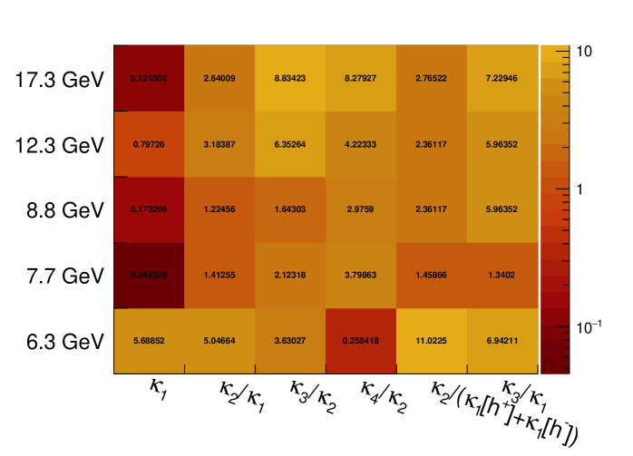
Figure 3: Difference (in $\%$) of unfolded and true values of quantities of the net-charge distribution where a sample from the model was treated as data (with statistics close to the experimental data) and the response matrix was built from FTFP-BERT.

5 Results

This section presents results on multiplicity and net-charge fluctuations of charged primary hadrons in inelastic interactions at $\sqrt{s_{NN}}=6.3,7.7,8.8,12.3$, and 17.3 GeV. In the first subsection, final corrected distributions of the considered charge combinations are presented along with model predictions and raw measured distributions, including detector effects. The second and third subsections present results on intensive quantities, which allow for a direct comparison with nucleus-nucleus collisions, and on factorial cumulants, which allow studying correlations.

5.1 Multiplicity and net-charge distributions

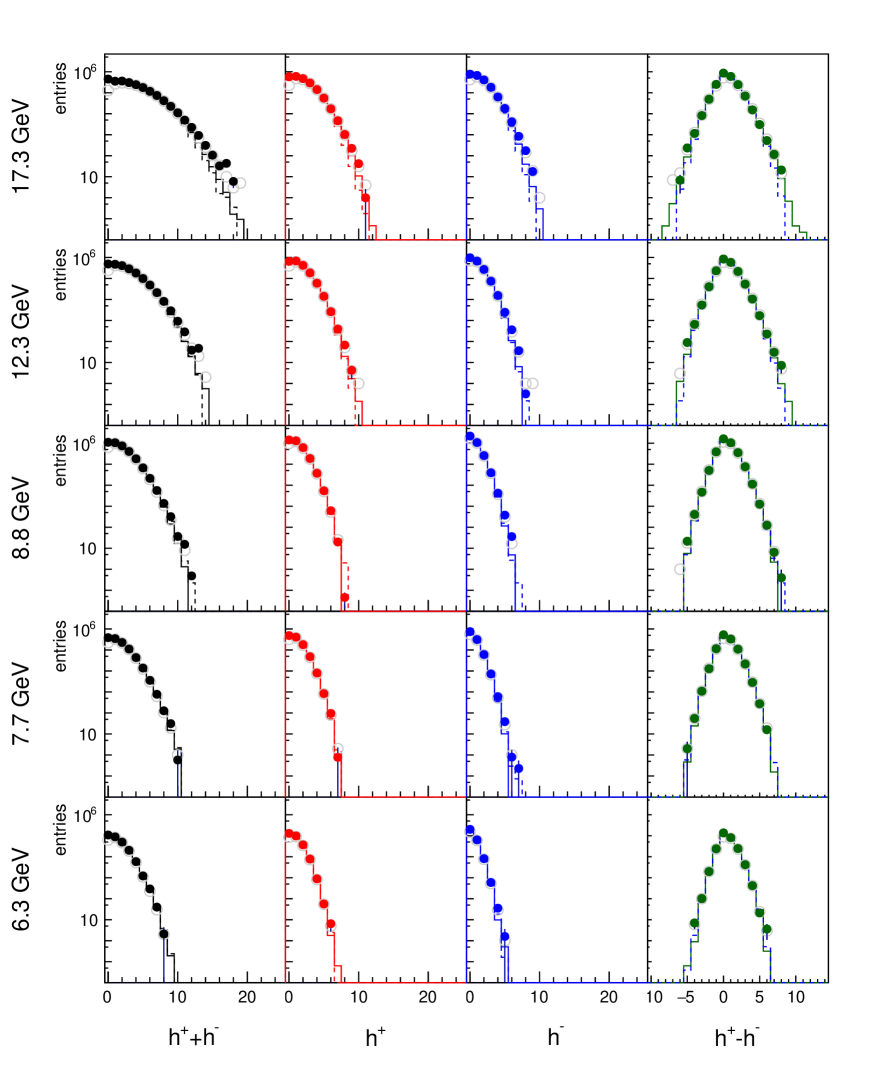
Figure 4: Multiplicity distributions of $h^{+}+h^{-}$, $h^{+}$, $h^{-}$, and $h^{+}-h^{-}$ in interactions at beam momenta 20, 31, 40, 80, and 158 . Open circles indicate raw, uncorrected data, whereas full circles show corrected distributions. Dashed and solid lines represent FTFP-BERT and model predictions, respectively.

Figure 4 shows corrected distributions of $h^{+}+h^{-}$, $h^{+}$, $h^{-}$, and $h^{+}-h^{-}$ (full circles) along with the raw measured distributions (open circles). The experimental results are compared to FTFP-BERT and models predictions (dashed and solid lines). The shape of the distribution is reproduced by the models in the case of positively and negatively charged hadrons. Small deviations from the model description in the tails of the distributions can be observed in the cases of $h^{+}+h^{-}$ and $h^{+}-h^{-}$.

5.2 Intensive quantities

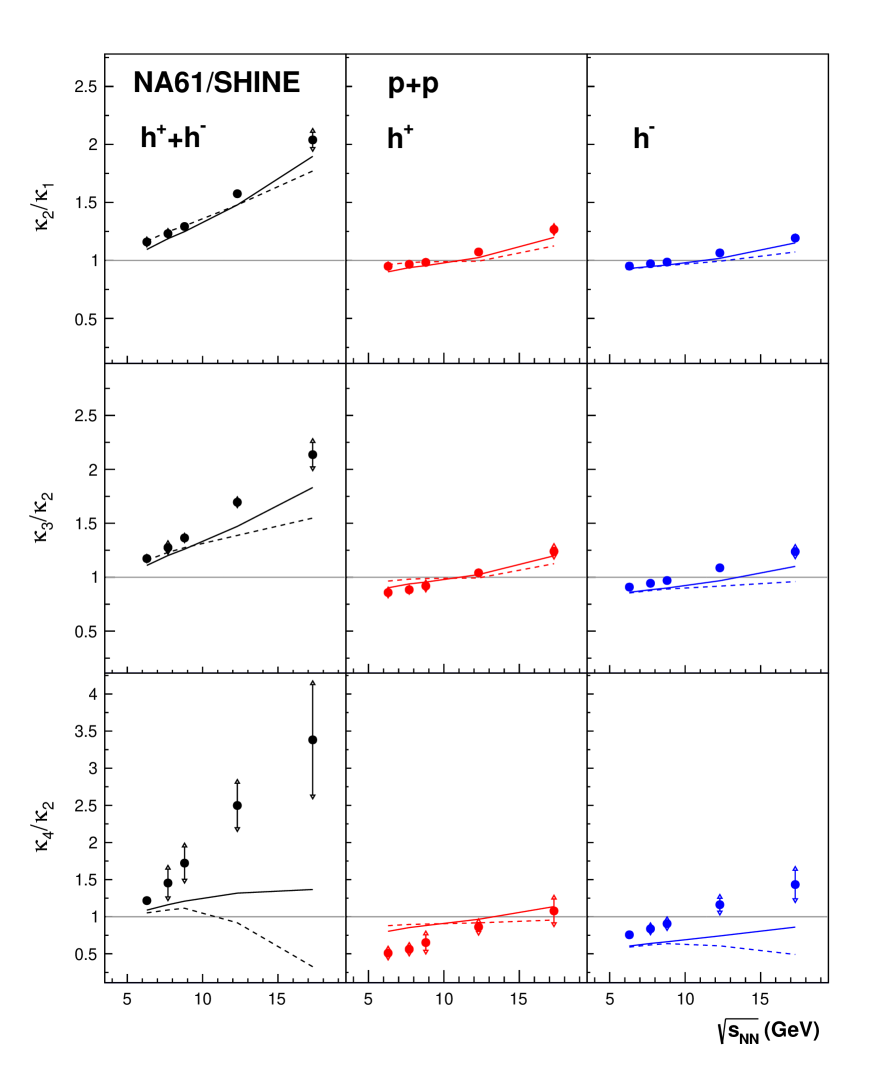
Figure 5: Energy dependence of intensive quantities of multiplicity distributions of $h^{+}+h^{-}$, $h^{+}$, and $h^{-}$ in interactions at at beam momenta 20, 31, 40, 80, and 158 . The statistical uncertainty is indicated with a color bar (often smaller than the marker), and systematic uncertainty is indicated with an arrow bar. Results are compared with (solid line) and FTFP-BERT (dashed line) predictions.

Results on the energy dependence of intensive quantities are presented in Fig. 5. All quantities increase with the interaction energy. The increase is the strongest for the sum of charges. All quantities obtained for summed charged hadrons remain above unity at all considered collision energies. This implies that fluctuations are enhanced with respect to Poisson. The same energy dependence can be observed in the case of positively and negatively charged hadrons, but the increase is much weaker with the signal crossing unity around $\sqrt{s_{NN}}\approx 10$ GeV except $\kappa_{4}/\kappa_{2}[h^{+}]$ where stays close to one for higher energies. The rise with interaction energy stays in agreement with the KNO-G scaling [7, 8, 9] observed in full kinematic acceptance [6]. However, another reason for the increasing strength of the signal is the increase of the analysis acceptance with interaction energy (see Table 1).

The results are compared with and FTFP-BERT models. Both models reproduce the experimental $\kappa_{2}/\kappa_{1}$ ratio but tend to underestimate $\kappa_{3}/\kappa_{2}$ and qualitatively disagree with $\kappa_{4}/\kappa_{2}$ for $h^{+}+h^{-}$ and $h^{-}$. It is unclear why, in the case of FTFP-BERT predictions, there is a maximum close to $\sqrt{s_{NN}}\approx 9$ GeV in the case of all and negatively charged hadrons.

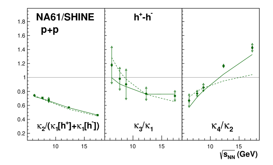
Figure 6: Energy dependence of intensive quantities of net-charge distribution in interactions at at beam momenta 20, 31, 40, 80, and 158 . The statistical uncertainty is indicated with a color bar (often smaller than the marker), and systematic uncertainty is indicated with an arrow bar. Results are compared with Epos (solid line) and FTFP-BERT (dashed line) predictions.

Figure 6 shows the energy dependence of net-charge fluctuations compared with model predictions. Second- and third-order cumulant ratios of $h^{+}-h^{-}$ distribution decrease with collision energy, whereas $\kappa_{4}[h^{+}-h^{-}]/\kappa_{2}[h^{+}-h^{-}]$ increases with collision energy. The measured signal for the majority of collected energies remains below unity. Both model predictions reproduce the observed decrease of $\kappa_{2}[h^{+}-h^{-}]/(\kappa_{1}[h^{+}]+\kappa_{1}[h^{-}])$ and $\kappa_{3}[h^{+}-h^{-}]/\kappa_{1}[h^{+}-h^{-}]$. Only $\kappa_{4}[h^{+}-h^{-}]/\kappa_{2}[h^{+}-h^{-}]$ at the two top energies is higher than unity. The model reproduces this rise with interaction energy whereas FTFP-BERT underestimates its strength.

5.3 Factorial cumulants

Factorial cumulants are quantities that allow extracting the correlation function of a given order (and without lower-order terms) from the measured distribution [19, 35].

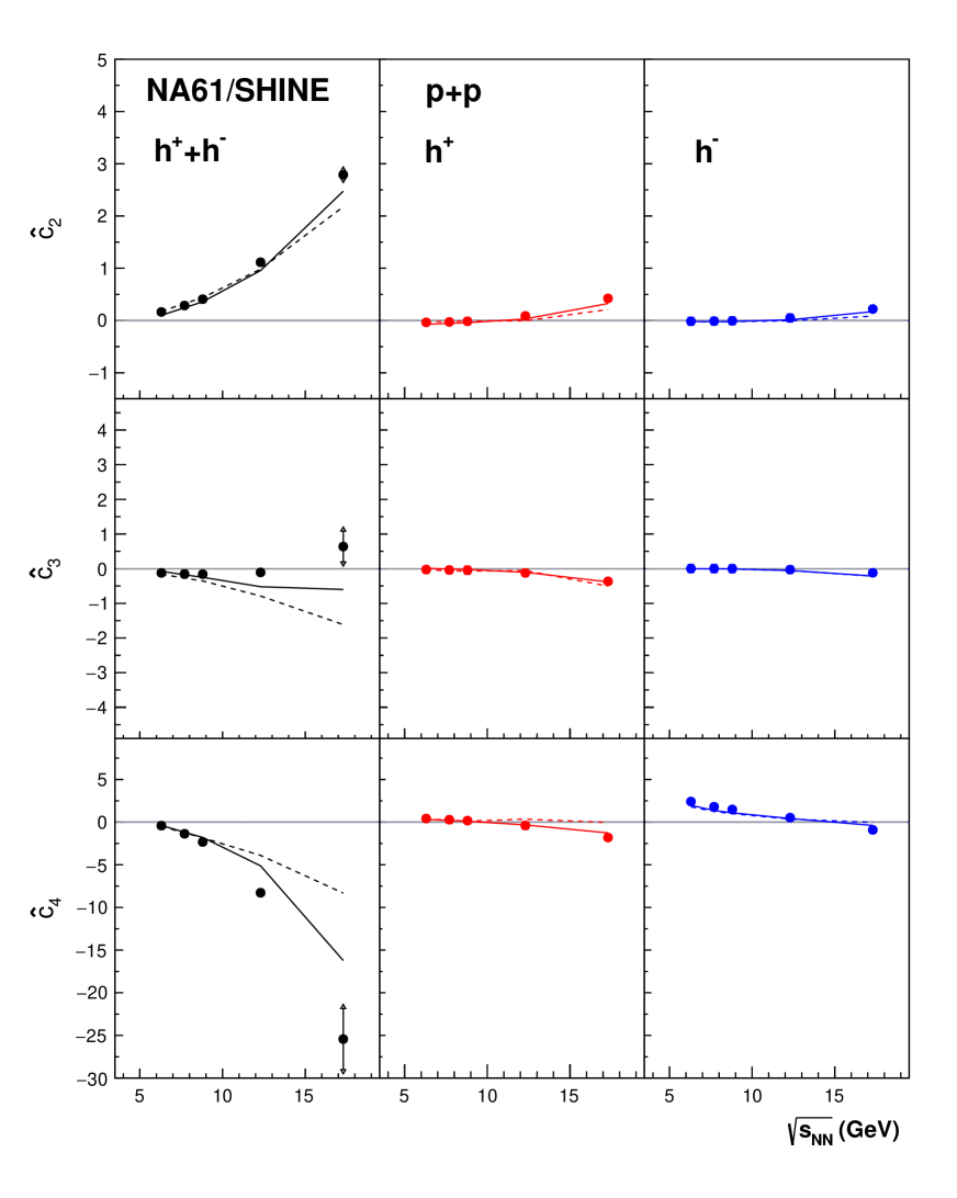
Figure 7: Energy dependence of factorial cumulants of multiplicity distributions of $h^{+}+h^{-}$, $h^{+}$, and $h^{-}$ in interactions at 20, 31, 40, 80, and 158 . The statistical uncertainty is indicated with a color bar (often smaller than the marker), and systematic uncertainty is indicated with an arrow bar. Results are compared with Epos (solid line) and FTFP-BERT (dashed line) predictions.

The energy dependence of factorial cumulants measured in interactions is presented in Fig. 7. Factorial cumulants of second- and third-order of distribution of $h^{+}+h^{-}$ increase with collision energy in contrast to $\hat{C_{4}}$ which decreases with collision energy. The $\hat{C}_{2}$ signal of $h^{+}$ and $h^{-}$ distributions slowly increases from zero to positive values at top energy. In contrast, $\hat{C}_{3}$ of $h^{+}$ and $h^{-}$ dsitributions similarly decreases with interaction energy. The $\hat{C}_{4}$ stays negative at all considered energies for all charged hadrons (separate charges also decrease with energy, but they are close to zero). Both models describe the energy dependence oh $\hat{C_{2}}[h^{+}+h^{-}]$ and qualitatively predict decrease of $\hat{C_{4}}[h^{+}+h^{-}]$. Increase of $\hat{C_{3}}[h^{+}+h^{-}]$ is not predicted by the models. Both models predict a decrease of $\hat{C_{3}}[h^{+}+h^{-}]$ with collision energy. Predictions for separate charges are in much better agreement with the data. and FTFP-BERT predict the observed dependences of factorial cumulants of $h^{+}$ and $h^{-}$ distributions. The FTFP-BERT predictions follow the data in a corser manner than .

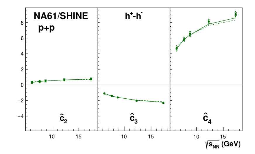
Figure 8: Energy dependence of factorial cumulants of net-charge distribution in interactions at beam momenta 20, 31, 40, 80, and 158 . The statistical uncertainty is indicated with a color bar (often smaller than the marker), and systematic uncertainty is indicated with an arrow bar. Results are compared with (solid line) and FTFP-BERT (dashed line) predictions.

Figure 8 shows the energy dependence of factorial cumulants of net-charge distribution. In all cases, factorial cumulants are far from zero, with $\hat{C}_{2}[h^{+}-h^{-}]$ and $\hat{C}_{4}[h^{+}-h^{-}]$ being positive at all interaction energies. The $\hat{C}_{3}[h^{+}-h^{-}]$ remains negative. Both models (and FTFP-BERT) quantitatively reproduce these dependencies.

6 Comparison with other systems

Quantitative comparison between systems is possible only if they were performed in a similar acceptance [36]. We leave such a comparison for future analysis of nucleus-nucleus collisions from the system-size scan of .

Nevertheless, qualitative comparisons between different experiments may provide useful information. The results on multiplicity fluctuations (studied with $\kappa_{2}/\kappa_{1}$ ratio) were already reported and discussed in Ref. [24]. Higher-order cumulant ratios of multiplicity distributions reported here are the first results provided in interactions for the considered energy range.

Results on the net-charge distribution were compared to results from the NA49 [37] and STAR [38, 39] experiments.

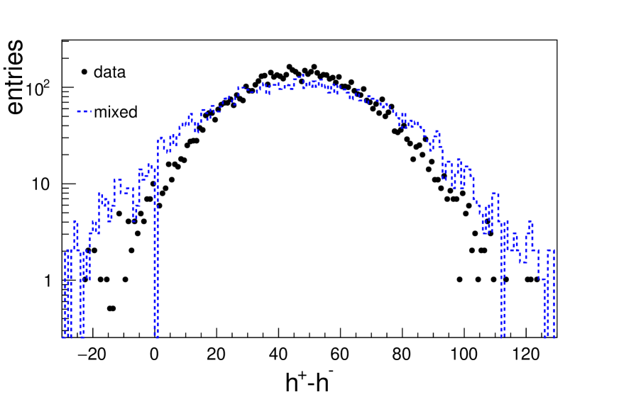
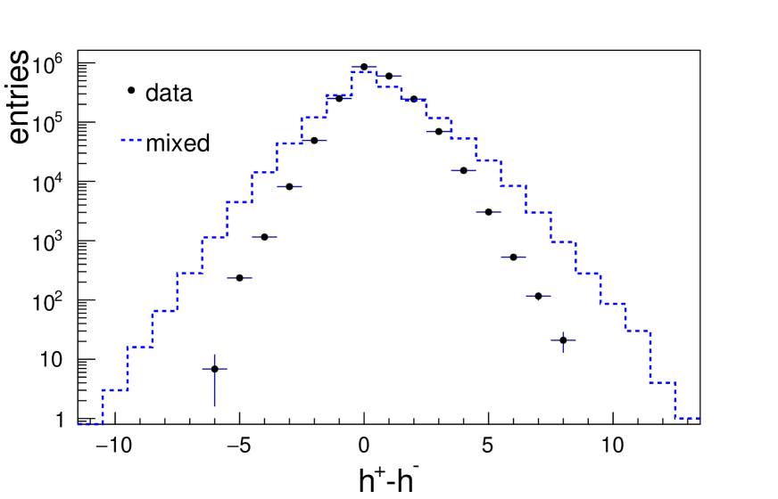
Figure 9: Net-charge distribution in the 10$\%$ most central Pb+Pb interactions at 158$A\,\mbox{Ge\kern-1.00006ptV}\!/\!c$ by NA49 (reproduced from Ref. [37]) (left) and in interactions at 158 by  (right). Both distributions are compared with mixed events (blue line) as defined in Ref. [37].

The left panel of Fig. 9 presents net-charge distribution measured by NA49 [37] in the 10$\%$ most central Pb+Pb interactions at beam momentum 158$A\,\mbox{Ge\kern-1.00006ptV}\!/\!c$. The NA49 analysis acceptance is comparable with the one used in this analysis. The NA49 data distribution (points) is compared with mixed events (blue line), which are constructed by randomly selecting particles from different events according to the multiplicity distribution measured for the data. The set of mixed events was prepared in the same way for interactions (see the right panel in Fig. 9). In both systems, mixed events distribution is wider than the data thus both distributions seem to be dominated by conservation laws. The net-charge distribution (around 7k central Pb+Pb interactions) provided by NA49 allows for estimating values of cumulant ratios for this reaction. Using formulas for statistical uncertainty estimation from Ref. [40], one may try to provide NA49 results with approximate statistical uncertainties. Thus, cumulant ratios in central Pb+Pb interactions at 158$A$ are $\kappa_{2}[h^{+}-h^{-}]/\kappa_{1}[h^{+}-h^{-}]=8.16\pm 0.17$ (stat), $\kappa_{3}[h^{+}-h^{-}]/\kappa_{2}[h^{+}-h^{-}]=0.9\pm 1.6$ (stat), and $\kappa_{4}[h^{+}-h^{-}]/\kappa_{2}[h^{+}-h^{-}]=21\pm 32$ (stat), approximately. The obtained ratios, within large uncertainties, are not too far from results in the 5$\%$ most central Au+Au collisions at $\sqrt{s_{NN}}=$ 19.6 GeV [38], which suggests that a qualitative comparison between STAR results and this analysis is possible.

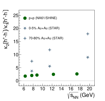
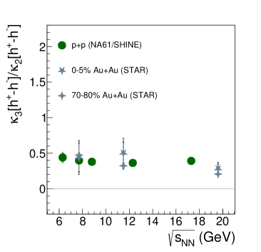
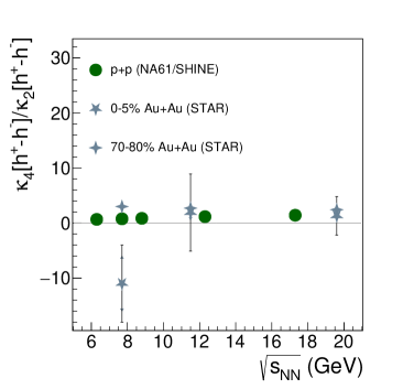
Figure 10: Net-charge cumulant ratios measured in interactions by and in central and pheripheral Au+Au interactions by STAR [38].

The comparison with Au+Au interactions [38] is presented in Fig. 10. It should be underlined that quantities $\kappa_{2}[h^{+}-h^{-}]/\kappa_{1}[h^{+}-h^{-}]$ and $\kappa_{3}[h^{+}-h^{-}]/\kappa_{2}[h^{+}-h^{-}]$ do not keep 0 and 1 as their reference values (see Sec. 2). Instead, for Skellam distribution $\kappa_{2}[h^{+}-h^{-}]/\kappa_{1}[h^{+}-h^{-}]$ should increase and $\kappa_{3}[h^{+}-h^{-}]/\kappa_{2}[h^{+}-h^{-}]$ should decrease with increasing multiplicity. In the case of scaled variance, interactions are well below central and peripheral Au+Au interactions. The difference may be driven mainly by the volume fluctuations, which are unavoidable with wide centrality bins. In GCE, volume fluctuations are modulated by the mean number of particles produced in a fixed $V$. Thus, the scaled variance should increase with increasing collision energy as more particles are produced at higher energies, explaining the observed energy dependence for Au+Au reactions. Such fluctuations are absent in the case of collisions, explaining a weaker increase with interaction energy.

The observed signal of $\kappa_{3}[h^{+}-h^{-}]/\kappa_{2}[h^{+}-h^{-}]$ and $\kappa_{4}[h^{+}-h^{-}]/\kappa_{2}[h^{+}-h^{-}]$ in Au+Au is close to interactions. Although volume fluctuations dependence of higher-order cumulant ratios remains, it is more elaborate (see Ref. [14]) and seems not to dominate the signal.

7 Summary

The experimental results on event-by-event fluctuations of multiplicities of all, positively, and negatively charged hadrons as well as net-electric charge (so-called net-charge) produced in inelastic proton-proton interactions at $\!\sqrt{s_{\mathrm{NN}}}$ = 6.3, 7.7, 8.8, 12.3, and 17.3 GeV are presented. The results were corrected for experimental biases with the unfolding technique. The corrected results were compared with and FTFP-BERT predictions. In general, both models qualitatively describe the measurements. The predictions are closer to the data. The KNO-G scaling and an increase in the analysis acceptance with collision energy probably caused the rise of cumulant ratios with the collision energy for multiplicity distributions ($h^{+}+h^{-}$, $h^{+}$, and $h^{-}$). The qualitative disagreement of FTFP-BERT for higher collision energies in $\kappa_{4}/\kappa_{2}$ can be seen for $h^{+}+h^{-}$ and $h^{-}$.

The most significant deviation of the measured signal to model predictions appears mostly for the sum of charges, indicating possible problems of models with describing correlations between charges, like resonances and conservation laws.

A qualitative comparison with Au+Au interactions does not indicate a significant difference between systems for higher-order cumulant ratios. Future comparisons are expected with precise NA61/SHINE results on nucleus-nucleus collisions.

Appendix A Appendix A

The numerical values of corrected distributions will be provided using the HEP Data [41, 42]. The numerical values of measured quantities are shown in Tabs. 4, 5, 6. The first uncertainty is statistical and the second is systematic. It should be underlined that $\kappa_{1}$ is not equivalent to the values measured by particle yields [21, 43] due to different event and track selections as well as different correction procedures.

$\sqrt{s_{NN}}$ (GeV)	quantity	$h^{+}+h^{-}$	$h^{+}$	$h^{-}$	$h^{+}-h^{-}$
6.3	$\kappa_{1}$	$1.0222\pm 0.0027\pm 0.071$	$0.7242\pm 0.0020\pm 0.038$	$0.3027\pm 0.0012\pm 0.025$	$0.4270\pm 0.0022\pm 0.012$
7.7	$\kappa_{1}$	$1.2381\pm 0.0015\pm 0.055$	$0.8365\pm 0.0011\pm 0.031$	$0.40468\pm 0.00070\pm 0.018$	$0.4325\pm 0.0012\pm 0.011$
8.8	$\kappa_{1}$	$1.3913\pm 0.0010\pm 0.16$	$0.91188\pm 0.00063\pm 0.096$	$0.48169\pm 0.00043\pm 0.057$	$0.43230\pm 0.00068\pm 0.033$
12.3	$\kappa_{1}$	$1.9373\pm 0.0017\pm 0.12$	$1.1922\pm 0.0010\pm 0.066$	$0.75133\pm 0.00077\pm 0.048$	$0.4493\pm 0.0010\pm 0.014$
17.3	$\kappa_{1}$	$2.6839\pm 0.0025\pm 0.11$	$1.5781\pm 0.0014\pm 0.055$	$1.1348\pm 0.0011\pm 0.039$	$0.4758\pm 0.0011\pm 0.0061$
6.3	$\kappa_{2}$	$1.1854\pm 0.0047\pm 0.042$	$0.6879\pm 0.0023\pm 0.014$	$0.2879\pm 0.0014\pm 0.023$	$0.7614\pm 0.0032\pm 0.030$
7.7	$\kappa_{2}$	$1.5250\pm 0.0029\pm 0.033$	$0.8088\pm 0.0013\pm 0.016$	$0.39328\pm 0.00090\pm 0.013$	$0.8777\pm 0.0017\pm 0.024$
8.8	$\kappa_{2}$	$1.7987\pm 0.0019\pm 0.19$	$0.89692\pm 0.00092\pm 0.070$	$0.47492\pm 0.00059\pm 0.053$	$0.9436\pm 0.0010\pm 0.056$
12.3	$\kappa_{2}$	$3.0518\pm 0.0041\pm 0.15$	$1.2795\pm 0.0019\pm 0.049$	$0.8002\pm 0.0013\pm 0.046$	$1.1072\pm 0.0017\pm 0.037$
17.3	$\kappa_{2}$	$5.4738\pm 0.0067\pm 0.15$	$2.0008\pm 0.0027\pm 0.065$	$1.3541\pm 0.0018\pm 0.025$	$1.2476\pm 0.0020\pm 0.041$
6.3	$\kappa_{3}$	$1.391\pm 0.015\pm 0.034$	$0.5903\pm 0.0056\pm 0.024$	$0.2616\pm 0.0028\pm 0.019$	$0.3340\pm 0.0060\pm 0.044$
7.7	$\kappa_{3}$	$1.944\pm 0.010\pm 0.071$	$0.7150\pm 0.0037\pm 0.026$	$0.3712\pm 0.0020\pm 0.010$	$0.3488\pm 0.0039\pm 0.033$
8.8	$\kappa_{3}$	$2.4540\pm 0.0071\pm 0.19$	$0.8241\pm 0.0024\pm 0.021$	$0.4605\pm 0.0014\pm 0.040$	$0.3571\pm 0.0024\pm 0.018$
12.3	$\kappa_{3}$	$5.173\pm 0.021\pm 0.13$	$1.3313\pm 0.0055\pm 0.049$	$0.8699\pm 0.0035\pm 0.028$	$0.4012\pm 0.0047\pm 0.027$
17.3	$\kappa_{3}$	$11.692\pm 0.042\pm 0.85$	$2.480\pm 0.010\pm 0.15$	$1.6751\pm 0.0064\pm 0.072$	$0.4877\pm 0.0064\pm 0.056$
6.3	$\kappa_{4}$	$1.027\pm 0.036\pm 0.059$	$0.742\pm 0.034\pm 0.15$	$2.628\pm 0.080\pm 0.27$	$0.877\pm 0.029\pm 0.17$
7.7	$\kappa_{4}$	$0.953\pm 0.017\pm 0.17$	$0.695\pm 0.016\pm 0.12$	$2.128\pm 0.032\pm 0.28$	$0.877\pm 0.014\pm 0.081$
8.8	$\kappa_{4}$	$0.957\pm 0.010\pm 0.28$	$0.7273\pm 0.0095\pm 0.25$	$1.908\pm 0.018\pm 0.45$	$0.9068\pm 0.0086\pm 0.13$
12.3	$\kappa_{4}$	$0.818\pm 0.013\pm 0.16$	$0.674\pm 0.011\pm 0.11$	$1.452\pm 0.019\pm 0.26$	$1.052\pm 0.012\pm 0.061$
17.3	$\kappa_{4}$	$0.618\pm 0.010\pm 0.14$	$0.539\pm 0.011\pm 0.10$	$1.058\pm 0.014\pm 0.19$	$1.143\pm 0.014\pm 0.078$
6.3	$\kappa_{2}/\kappa_{1}$	$1.1596\pm 0.0040\pm 0.041$	$0.9499\pm 0.0028\pm 0.036$	$0.9511\pm 0.0030\pm 0.0051$	$1.7831\pm 0.0094\pm 0.028$
7.7	$\kappa_{2}/\kappa_{1}$	$1.2317\pm 0.0019\pm 0.042$	$0.9669\pm 0.0014\pm 0.028$	$0.9718\pm 0.0014\pm 0.012$	$2.0295\pm 0.0054\pm 0.011$
8.8	$\kappa_{2}/\kappa_{1}$	$1.2929\pm 0.0011\pm 0.014$	$0.98359\pm 0.00092\pm 0.031$	$0.98596\pm 0.00088\pm 0.010$	$2.1828\pm 0.0036\pm 0.039$
12.3	$\kappa_{2}/\kappa_{1}$	$1.5753\pm 0.0021\pm 0.021$	$1.0732\pm 0.0014\pm 0.019$	$1.0650\pm 0.0013\pm 0.0070$	$2.4641\pm 0.0049\pm 0.067$
17.3	$\kappa_{2}/\kappa_{1}$	$2.0395\pm 0.0027\pm 0.098$	$1.2678\pm 0.0017\pm 0.049$	$1.1933\pm 0.0013\pm 0.032$	$2.6221\pm 0.0062\pm 0.057$
6.3	$\kappa_{3}/\kappa_{2}$	$1.1731\pm 0.0093\pm 0.037$	$0.8582\pm 0.0064\pm 0.048$	$0.9086\pm 0.0068\pm 0.0081$	$0.4387\pm 0.0075\pm 0.077$
7.7	$\kappa_{3}/\kappa_{2}$	$1.2748\pm 0.0048\pm 0.063$	$0.8841\pm 0.0035\pm 0.041$	$0.9438\pm 0.0034\pm 0.026$	$0.3973\pm 0.0043\pm 0.050$
8.8	$\kappa_{3}/\kappa_{2}$	$1.3643\pm 0.0029\pm 0.042$	$0.9189\pm 0.0020\pm 0.054$	$0.9696\pm 0.0020\pm 0.025$	$0.3785\pm 0.0026\pm 0.044$
12.3	$\kappa_{3}/\kappa_{2}$	$1.6952\pm 0.0051\pm 0.049$	$1.0405\pm 0.0032\pm 0.032$	$1.0871\pm 0.0031\pm 0.028$	$0.3624\pm 0.0042\pm 0.028$
17.3	$\kappa_{3}/\kappa_{2}$	$2.1360\pm 0.0061\pm 0.14$	$1.2396\pm 0.0039\pm 0.071$	$1.2371\pm 0.0036\pm 0.065$	$0.3909\pm 0.0051\pm 0.033$
6.3	$\kappa_{4}/\kappa_{2}$	$1.217\pm 0.045\pm 0.023$	$0.510\pm 0.024\pm 0.092$	$0.757\pm 0.024\pm 0.013$	$0.668\pm 0.022\pm 0.098$
7.7	$\kappa_{4}/\kappa_{2}$	$1.454\pm 0.028\pm 0.24$	$0.562\pm 0.013\pm 0.089$	$0.837\pm 0.013\pm 0.079$	$0.769\pm 0.013\pm 0.048$
8.8	$\kappa_{4}/\kappa_{2}$	$1.722\pm 0.019\pm 0.27$	$0.6523\pm 0.0087\pm 0.15$	$0.9064\pm 0.0087\pm 0.090$	$0.8557\pm 0.0082\pm 0.060$
12.3	$\kappa_{4}/\kappa_{2}$	$2.498\pm 0.040\pm 0.35$	$0.862\pm 0.015\pm 0.11$	$1.162\pm 0.015\pm 0.14$	$1.165\pm 0.014\pm 0.027$
17.3	$\kappa_{4}/\kappa_{2}$	$3.382\pm 0.058\pm 0.79$	$1.078\pm 0.022\pm 0.21$	$1.433\pm 0.020\pm 0.24$	$1.426\pm 0.018\pm 0.062$

Table 4: Numerical values of cumulants and cumulant ratios of $h^{+}+h^{-}$, $h^{+}$, $h^{-}$, and $h^{+}-h^{-}$.

$\sqrt{s_{NN}}$ (GeV)	quantity	$h^{+}+h^{-}$	$h^{+}$	$h^{-}$	$h^{+}-h^{-}$
6.3	$\hat{C_{2}}$	$0.1631\pm 0.0040\pm 0.029$	$-0.0363\pm 0.0021\pm 0.027$	$-0.01481\pm 0.00090\pm 0.0026$	$0.3344\pm 0.0033\pm 0.020$
7.7	$\hat{C_{2}}$	$0.2869\pm 0.0024\pm 0.037$	$-0.0277\pm 0.0012\pm 0.024$	$-0.01140\pm 0.00056\pm 0.0051$	$0.4452\pm 0.0017\pm 0.014$
8.8	$\hat{C_{2}}$	$0.4074\pm 0.0016\pm 0.029$	$-0.01496\pm 0.00084\pm 0.027$	$-0.00676\pm 0.00042\pm 0.0049$	$0.5113\pm 0.0011\pm 0.023$
12.3	$\hat{C_{2}}$	$1.1145\pm 0.0038\pm 0.038$	$0.0873\pm 0.0017\pm 0.018$	$0.0489\pm 0.0010\pm 0.0017$	$0.6579\pm 0.0016\pm 0.030$
17.3	$\hat{C_{2}}$	$2.7899\pm 0.0064\pm 0.15$	$0.4226\pm 0.0026\pm 0.060$	$0.2194\pm 0.0015\pm 0.027$	$0.7718\pm 0.0021\pm 0.035$
6.3	$\hat{C_{3}}$	$-0.1211\pm 0.0066\pm 0.024$	$-0.0249\pm 0.0028\pm 0.020$	$0.00331\pm 0.00075\pm 0.0011$	$-1.0962\pm 0.0096\pm 0.11$
7.7	$\hat{C_{3}}$	$-0.1547\pm 0.0050\pm 0.014$	$-0.0384\pm 0.0018\pm 0.014$	$0.00069\pm 0.00072\pm 0.00024$	$-1.4194\pm 0.0057\pm 0.085$
8.8	$\hat{C_{3}}$	$-0.1596\pm 0.0040\pm 0.057$	$-0.0429\pm 0.0013\pm 0.0031$	$-0.00089\pm 0.00051\pm 0.0026$	$-1.6091\pm 0.0035\pm 0.12$
12.3	$\hat{C_{3}}$	$-0.108\pm 0.012\pm 0.10$	$-0.1228\pm 0.0028\pm 0.021$	$-0.0280\pm 0.0017\pm 0.014$	$-2.0217\pm 0.0062\pm 0.099$
17.3	$\hat{C_{3}}$	$0.639\pm 0.029\pm 0.56$	$-0.3658\pm 0.0056\pm 0.059$	$-0.1177\pm 0.0033\pm 0.030$	$-2.3036\pm 0.0087\pm 0.099$
6.3	$\hat{C_{4}}$	$-0.411\pm 0.025\pm 0.067$	$0.421\pm 0.017\pm 0.12$	$2.410\pm 0.073\pm 0.28$	$4.686\pm 0.046\pm 0.36$
7.7	$\hat{C_{4}}$	$-1.365\pm 0.024\pm 0.12$	$0.2824\pm 0.0052\pm 0.069$	$1.799\pm 0.026\pm 0.26$	$5.844\pm 0.026\pm 0.32$
8.8	$\hat{C_{4}}$	$-2.329\pm 0.021\pm 0.30$	$0.1773\pm 0.0032\pm 0.18$	$1.479\pm 0.014\pm 0.46$	$6.550\pm 0.017\pm 0.40$
12.3	$\hat{C_{4}}$	$-8.275\pm 0.080\pm 0.19$	$-0.393\pm 0.010\pm 0.033$	$0.5268\pm 0.0085\pm 0.21$	$8.128\pm 0.030\pm 0.36$
17.3	$\hat{C_{4}}$	$-25.43\pm 0.19\pm 4.1$	$-1.803\pm 0.030\pm 0.40$	$-0.905\pm 0.013\pm 0.14$	$9.086\pm 0.041\pm 0.36$

Table 5: Numerical values of factorial cumulants of $h^{+}+h^{-}$, $h^{+}$, $h^{-}$, and $h^{+}-h^{-}$.

$\sqrt{s_{NN}}$ (GeV)	quantity	$h^{+}-h^{-}$
6.3	$\kappa_{2}[h^{+}-h^{-}]/(\kappa_{1}[h^{+}]+\kappa_{1}[h^{-}])$	$0.7431\pm 0.0032\pm 0.017$
7.7	$\kappa_{2}[h^{+}-h^{-}]/(\kappa_{1}[h^{+}]+\kappa_{1}[h^{-}])$	$0.7072\pm 0.0017\pm 0.0088$
8.8	$\kappa_{2}[h^{+}-h^{-}]/(\kappa_{1}[h^{+}]+\kappa_{1}[h^{-}])$	$0.6771\pm 0.0010\pm 0.039$
12.3	$\kappa_{2}[h^{+}-h^{-}]/(\kappa_{1}[h^{+}]+\kappa_{1}[h^{-}])$	$0.5697\pm 0.0017\pm 0.014$
17.3	$\kappa_{2}[h^{+}-h^{-}]/(\kappa_{1}[h^{+}]+\kappa_{1}[h^{-}])$	$0.4599\pm 0.0020\pm 0.010$
6.3	$\kappa_{3}[h^{+}-h^{-}]/\kappa_{1}[h^{+}-h^{-}]$	$1.177\pm 0.020\pm 0.27$
7.7	$\kappa_{3}[h^{+}-h^{-}]/\kappa_{1}[h^{+}-h^{-}]$	$0.981\pm 0.011\pm 0.17$
8.8	$\kappa_{3}[h^{+}-h^{-}]/\kappa_{1}[h^{+}-h^{-}]$	$0.9012\pm 0.0064\pm 0.22$
12.3	$\kappa_{3}[h^{+}-h^{-}]/\kappa_{1}[h^{+}-h^{-}]$	$0.7665\pm 0.0091\pm 0.098$
17.3	$\kappa_{3}[h^{+}-h^{-}]/\kappa_{1}[h^{+}-h^{-}]$	$0.735\pm 0.010\pm 0.078$

Table 6: Numerical values of cumulant ratio combinations which are intensive for net-charge.

The Collaboration

H. Adhikary ¹¹, P. Adrich ¹³, K.K. Allison ²⁴, N. Amin ⁴, E.V. Andronov ²⁰, I.-C. Arsene ¹⁰, M. Bajda ¹⁴, Y. Balkova ¹⁶, D. Battaglia ²³, A. Bazgir ¹¹, S. Bhosale ¹², M. Bielewicz ¹³, A. Blondel ³, M. Bogomilov ², Y. Bondar ¹¹, A. Borucka¹⁹, A. Brandin²⁰, W. Bryliński ¹⁹, J. Brzychczyk ¹⁴, M. Buryakov ²⁰, A.F. Camino²⁶, M. Ćirković ²¹, M. Csanád ⁶, J. Cybowska ¹⁹, T. Czopowicz ¹¹, C. Dalmazzone ³, N. Davis ¹², A. Dmitriev ²⁰, P. von Doetinchem ²⁵, W. Dominik ¹⁷, J. Dumarchez ³, R. Engel ⁴, G.A. Feofilov ²⁰, L. Fields ²³, Z. Fodor ^5,18, M. Friend ⁷, M. Gaździcki ¹¹, O. Golosov ²⁰, V. Golovatyuk ²⁰, M. Golubeva ²⁰, K. Grebieszkow ¹⁹, F. Guber ²⁰, S.N. Igolkin²⁰, S. Ilieva ², A. Ivashkin ²⁰, A. Izvestnyy ²⁰, N. Kargin²⁰, N. Karpushkin ²⁰, E. Kashirin ²⁰, M. Kiełbowicz ¹², V.A. Kireyeu ²⁰, R. Kolesnikov ²⁰, D. Kolev ², Y. Koshio⁸, V.N. Kovalenko ²⁰, S. Kowalski ¹⁶, B. Kozłowski ¹⁹, A. Krasnoperov ²⁰, W. Kucewicz ¹⁵, M. Kuchowicz ¹⁸, M. Kuich ¹⁷, A. Kurepin ²⁰, A. László ⁵, M. Lewicki ¹⁸, G. Lykasov ²⁰, V.V. Lyubushkin ²⁰, M. Maćkowiak-Pawłowska ¹⁹, Z. Majka ¹⁴, A. Makhnev ²⁰, B. Maksiak ¹³, A.I. Malakhov ²⁰, A. Marcinek ¹², A.D. Marino ²⁴, H.-J. Mathes ⁴, T. Matulewicz ¹⁷, V. Matveev ²⁰, G.L. Melkumov ²⁰, A. Merzlaya ¹⁰, Ł. Mik ¹⁵, S. Morozov ²⁰, Y. Nagai ⁶, T. Nakadaira ⁷, M. Naskręt ¹⁸, S. Nishimori ⁷, A. Olivier ²³, V. Ozvenchuk ¹², O. Panova ¹¹, V. Paolone ²⁶, O. Petukhov ²⁰, I. Pidhurskyi ¹¹, R. Płaneta ¹⁴, P. Podlaski ¹⁷, B.A. Popov ^20,3, B. Pórfy ^5,6, D.S. Prokhorova ²⁰, D. Pszczel ¹³, S. Puławski ¹⁶, J. Puzović^21†, R. Renfordt ¹⁶, L. Ren ²⁴, V.Z. Reyna Ortiz ¹¹, D. Röhrich⁹, E. Rondio ¹³, M. Roth ⁴, Ł. Rozpłochowski ¹², B.T. Rumberger ²⁴, M. Rumyantsev ²⁰, A. Rustamov ¹, M. Rybczynski ¹¹, A. Rybicki ¹², D. Rybka¹³, K. Sakashita ⁷, K. Schmidt ¹⁶, A.Yu. Seryakov ²⁰, P. Seyboth ¹¹, U.A. Shah ¹¹, Y. Shiraishi⁸, A. Shukla ²⁵, M. Słodkowski ¹⁹, P. Staszel ¹⁴, G. Stefanek ¹¹, J. Stepaniak ¹³, M. Strikhanov²⁰, Ł. Świderski ¹³, J. Szewiński ¹³, R. Szukiewicz ¹⁸, A. Taranenko ²⁰, A. Tefelska ¹⁹, D. Tefelski ¹⁹, V. Tereshchenko²⁰, R. Tsenov ², L. Turko ¹⁸, T.S. Tveter ¹⁰, M. Unger ⁴, M. Urbaniak ¹⁶, F.F. Valiev ²⁰, D. Veberič ⁴, V.V. Vechernin ²⁰, O. Vitiuk ¹⁸, V. Volkov ²⁰, A. Wickremasinghe ²², K. Witek ¹⁵, K. Wójcik ¹⁶, O. Wyszyński ¹¹, A. Zaitsev ²⁰, E. Zherebtsova ¹⁸, E.D. Zimmerman ²⁴, A. Zviagina ²⁰, and R. Zwaska ^22
 
† deceased

¹ National Nuclear Research Center, Baku, Azerbaijan
² Faculty of Physics, University of Sofia, Sofia, Bulgaria
³ LPNHE, Sorbonne University, CNRS/IN2P3, Paris, France
⁴ Karlsruhe Institute of Technology, Karlsruhe, Germany
⁵ HUN-REN Wigner Research Centre for Physics, Budapest, Hungary
⁶ Eötvös Loránd University, Budapest, Hungary
⁷ Institute for Particle and Nuclear Studies, Tsukuba, Japan
⁸ Okayama University, Japan
⁹ University of Bergen, Bergen, Norway
¹⁰ University of Oslo, Oslo, Norway
¹¹ Jan Kochanowski University, Kielce, Poland
¹² Institute of Nuclear Physics, Polish Academy of Sciences, Cracow, Poland
¹³ National Centre for Nuclear Research, Warsaw, Poland
¹⁴ Jagiellonian University, Cracow, Poland
¹⁵ AGH - University of Science and Technology, Cracow, Poland
¹⁶ University of Silesia, Katowice, Poland
¹⁷ University of Warsaw, Warsaw, Poland
¹⁸ University of Wrocław, Wrocław, Poland
¹⁹ Warsaw University of Technology, Warsaw, Poland
²⁰ Affiliated with an institution covered by a cooperation agreement with CERN
²¹ University of Belgrade, Belgrade, Serbia
²² Fermilab, Batavia, USA
²³ University of Notre Dame, Notre Dame, USA
²⁴ University of Colorado, Boulder, USA
²⁵ University of Hawaii at Manoa, Honolulu, USA
²⁶ University of Pittsburgh, Pittsburgh, USA

References

- [1] N. Abgrall et al., [NA61/SHINE Collab.] JINST 9 (2014) P06005.
- [2] A. Aduszkiewicz, [NA61/SHINE Collab.], “Report from the NA61/SHINE experiment at the CERN SPS,” Tech. Rep. CERN-SPSC-2018-029. SPSC-SR-239, CERN, 2018. https://cds.cern.ch/record/2642286.
- [3] M. A. Stephanov, K. Rajagopal, and E. V. Shuryak Phys.Rev. D60 (1999) 114028, arXiv:hep-ph/9903292 [hep-ph].
- [4] E. V. Shuryak and M. A. Stephanov Phys.Rev. C63 (2001) 064903, arXiv:hep-ph/0010100 [hep-ph].
- [5] P. Braun-Munzinger, B. Friman, K. Redlich, A. Rustamov, and J. Stachel Nuclear Physics A 1008 (2021) 122141.
- [6] H. Heiselberg Phys. Rept. 351 (2001) 161.
- [7] Z. Koba, H. B. Nielsen, and P. Olesen Nucl. Phys. B40 (1972) 317–334.
- [8] A. Golokhvastov Phys. Atom. Nucl. 64 (2001) 1841–1855.
- [9] A. Golokhvastov Phys. Atom. Nucl. 64 (2001) 84–97.
- [10] O. Savchuk, R. V. Poberezhnyuk, V. Vovchenko, and M. I. Gorenstein Phys. Rev. C 101 no. 2, (2020) 024917, arXiv:1911.03426 [hep-ph].
- [11] M. Asakawa and M. Kitazawa Prog. Part. Nucl. Phys. 90 (2016) 299–342, arXiv:1512.05038 [nucl-th].
- [12] M. Gorenstein and M. Gazdzicki Phys. Rev. C84 (2011) 014904.
- [13] A. Bialas, M. Bleszynski, and W. Czyz Nucl. Phys. B111 (1976) 461.
- [14] V. Begun arXiv:1606.05358 [nucl-th].
- [15] M. I. Gorenstein J.Phys. G35 (2008) 125102, arXiv:0806.2804 [nucl-th].
- [16] V. Begun, M. I. Gorenstein, M. Hauer, V. Konchakovski, and O. Zozulya Phys.Rev. C74 (2006) 044903, arXiv:nucl-th/0606036 [nucl-th].
- [17] A. Bzdak, S. Esumi, V. Koch, J. Liao, M. Stephanov, and N. Xu Phys. Rept. 853 (2020) 1–87, arXiv:1906.00936 [nucl-th].
- [18] B. Ling and M. A. Stephanov Phys. Rev. C 93 no. 3, (2016) 034915, arXiv:1512.09125 [nucl-th].
- [19] A. Bzdak, V. Koch, and N. Strodthoff Phys. Rev. C 95 no. 5, (2017) 054906, arXiv:1607.07375 [nucl-th].
- [20] N. Abgrall et al., [NA61/SHINE Collab.] Eur. Phys. J. C74 (2014) 2794.
- [21] A. Aduszkiewicz et al., [NA61/SHINE Collab.] Eur. Phys. J. C77 no. 10, (2017) 671.
- [22] NA61/SHINE common system-size analysis region https://edms.cern.ch/document/2487456.
- [23] T. Adye Proceedings of the PHYSTAT 2011 Workshop on Statistical Issues Related to Discovery Claims in Search Experiments and Unfolding, CERN, Geneva, Switzerland, CERN-2011-006 (2011) 313–318. http://hepunx.rl.ac.uk/~adye/software/unfold/RooUnfold.html.
- [24] A. Aduszkiewicz et al., [NA61/SHINE Collab.] Eur. Phys. J. C76 (2016) 635.
- [25] NA61/SHINE acceptance for \ppanalysis https://edms.cern.ch/document/2228711/1.
- [26] K. Werner Nucl. Phys. Proc. Suppl. 175-176 (2008) 81–87.
- [27] T. Pierog and K. Werner Nucl.Phys.Proc.Suppl. 196 (2009) 102–105, arXiv:0905.1198 [hep-ph].
- [28] J. Allison et al., [GEANT4 Collab.] Nuclear Instruments and Methods in Physics Research Section A: Accelerators, Spectrometers, Detectors and Associated Equipment 835 (2016) 186–225. https://www.sciencedirect.com/science/article/pii/S0168900216306957.
- [29] S. Agostinelli et al., [GEANT4 Collab.] Nucl. Instrum. Meth. A506 (2003) 250.
- [30] J. Allison et al., [GEANT4 Collab.] IEEE Trans.Nucl.Sci. 53 (2006) 270.
- [31] J. Allison et al. Nucl. Instrum. Meth. A 835 (2016) 186–225.
- [32] C. F. Brun R., “Geant detector description and simulation tool, cern program library long writeup w5013,” 1993. http://wwwasdoc.web.cern.ch/wwwasdoc/geant/geantall.html.
- [33] B. Efron The Annals of Statistics 7 (1979) 1–26.
- [34] T. C. Hesterberg, D. S. Moore, S. Monaghan, A. Clipson, and R. Epstein, “Bootstrap methods and permutation tests,” 2005. http://bcs.whfreeman.com/ips5e/content/cat_080/pdf/moore14.pdf.
- [35] M. Kitazawa and X. Luo Phys. Rev. C 96 no. 2, (2017) 024910, arXiv:1704.04909 [nucl-th].
- [36] V. Vovchenko, O. Savchuk, R. V. Poberezhnyuk, M. I. Gorenstein, and V. Koch Phys. Lett. B 811 (2020) 135868, arXiv:2003.13905 [hep-ph].
- [37] C. Alt et al., [NA49 Collab.] Phys. Rev. C 70 (2004) 064903, arXiv:nucl-ex/0406013.
- [38] L. Adamczyk et al., [STAR Collab.] Phys. Rev. Lett. 113 (2014) 092301, arXiv:1402.1558 [nucl-ex].
- [39] A. Pandav, [STAR Collab.] Nucl. Phys. A 1005 (2021) 121936, arXiv:2003.12503 [nucl-ex].
- [40] X. Luo J. Phys. G 39 (2012) 025008, arXiv:1109.0593 [physics.data-an].
- [41] E. Maguire, L. Heinrich, and G. Watt J. Phys. Conf. Ser. 898 no. 10, (2017) 102006, arXiv:1704.05473 [hep-ex].
- [42] HEPData repository, https://www.hepdata.net.
- [43] N. Abgrall et al., [NA61/SHINE Collab.] Eur. Phys. J. C 74 no. 3, (2014) 2794, arXiv:1310.2417 [hep-ex].
The \NASixtyOneCollaboration