New Convergence Analysis of GMRES with
Weighted Norms, Preconditioning and Deflation,
Leading to a New Deflation Space

Abstract

New convergence bounds are presented for weighted, preconditioned, and deflated GMRES for the solution of large, sparse, nonsymmetric linear systems, where it is assumed that the symmetric part of the coefficient matrix is positive definite. The new bounds are sufficiently explicit to indicate how to choose the preconditioner and the deflation space to accelerate the convergence. One such choice of deflating space is presented, and numerical experiments illustrate the effectiveness of such space.

Keywords: linear solver, convergence analysis, domain decomposition, deflation space, preconditioning, deflation

AMS Subject Classification: 65F10, 65Y05, 68W40

1 Introduction

Our aim in this paper is to study effective solutions of linear systems of the form

$$\mathbf{A}\mathbf{x}=\mathbf{b},\quad\mathbf{A}\in\mathbb{K}^{n\times n},$$ (1)

where $\mathbb{K}=\mathbb{R}$ or $\mathbb{C}$ and $\mathbf{A}$ is a large sparse nonsingular matrix. Particular emphasis will be on the cases where $\mathbf{A}$ has a positive definite Hermitian part. We refer to such matrices $\mathbf{A}$ as positive definite matrices.

We are interested in studying effective approaches to accelerate the convergence of the well-known and widely used GMRES method [19] for the solution of linear systems. There are essentially three components for a successful strategy for this accelerations, which can be used alone or be combined:

• preconditioning,

• weighting,

• deflating.

Standard references for preconditioning include [2, 18, 20]; for weighted GMRES [8, 10, 14]; and for deflation [4, 6, 9, 12], and more recently [11]. Here, we denote the weighted preconditioned and deflated GMRES algorithm as WPD-GMRES, and corresponds to the case where all three acceleration tools are used.

Our objective in this paper is to propose a new convergence bound for WPD-GMRES that is sufficiently explicit to indicate how to choose the preconditioner, weight matrix, and especially deflation spaces. The new results generalize those in [22] where deflation was not considered. Here also, special emphasis is on Hermitian preconditioning and on applying WPD-GMRES in the preconditioner norm, an idea already present in [5, 25].

In particular, in Section 6, we present a result explicitly giving conditions on the preconditioner and the deflation spaces so as to assure fast convergence. Then, in Section 7, we propose a new deflation space which is inspired by this new bound. Numerical experiments in Section 8 illustrate the new results with the choice of new space, and show its effectiveness.

In part inspired by the success of the GenEO coarse space [23, 24], and as already mentioned, by the new bounds we obtain, we use as a deflation space, appropriately chosen eigenvectors of the generalized eigenvalue problem $\mathbf{N}\mathbf{z}=\lambda\mathbf{M}\mathbf{z}$, where $\mathbf{M}$ is the Hermitian part of $\mathbf{A}$, which is assumed to be positive definite, and $\mathbf{N}$ is the skew-Hermitian part of $\mathbf{A}$.

2 Preliminaries

We begin by stating some results for weighted GMRES for singular systems. As we describe in the next section, deflating produces a consistent singular system and thus, analyzing the singular case will be useful for our analysis of deflated GMRES.

Weighted GMRES is the version of GMRES in which a general inner product $\langle\cdot,\cdot\rangle_{\mathbf{W}}$ replaces the Euclidean inner product [10]. The Hermitian positive definite (hpd) matrix $\mathbf{W}$ such that $\langle\mathbf{x},\mathbf{y}\rangle_{\mathbf{W}}=\langle\mathbf{W}\mathbf{x},\mathbf{y}\rangle$ will be referred to as the weight matrix. The user inputs an initial vector $\mathbf{x}_{0}\in\mathbb{K}^{n}$. The approximate solution at iteration $i$ is then characterized by

$$\|\mathbf{r}_{i}\|_{\mathbf{W}}=\operatorname{min}\left\{\|\mathbf{b}-\mathbf{A}\mathbf{x}\|_{\mathbf{W}};\,{\mathbf{x}\in\mathbf{x}_{0}+\mathcal{K}_{i}}\right\},$$ (2)

where $\mathcal{K}_{i}$ is the Krylov subspace

$$\mathcal{K}_{i}=\mathcal{K}_{i}(\mathbf{r}_{0},\mathbf{A})=\operatorname{span}\{\mathbf{r}_{0},\mathbf{A}\mathbf{r}_{0},\dots,\mathbf{A}^{i-1}\mathbf{r}_{0}\};\quad\mathbf{r}_{0}=\mathbf{b}-\mathbf{A}\mathbf{x}_{0}.$$ (3)

GMRES for singular systems is studied in [3] and [15] (where GCR is also considered). A very useful result is recalled in Theorem 1 with a straightforward generalization to weighted GMRES. The proof of [3, Theorem 2.6] applies here with the change of inner product.

Theorem 1.

Suppose that $\operatorname{range}(\mathbf{A})\cap\operatorname{ker}(\mathbf{A})=\{0\}$. If $\mathbf{A}\mathbf{x}=\mathbf{b}$ is consistent, i.e., if it admits a solution, then weighted GMRES determines a solution without breakdown at some step and breaks down at the next step through degeneracy of the Krylov subspace.

The takeaway from the theorem is that for consistent linear systems, under the condition that $\operatorname{range}(\mathbf{A})\cap\operatorname{ker}(\mathbf{A})=\{\mathbf{0}\}$, we can proceed through the iterations in the same manner as with nonsingular systems. In exact arithmetic, the characterization (2) of the iterate $\mathbf{x}_{i}$ remains valid until the algorithm breaks down, at which point the exact solution has been found.

We continue in this preliminaries section by reviewing properties of the generalized eigenvalue problem we use for our new deflation space.

Lemma 1.

Let us assume that $\mathbf{M}$ and $\mathbf{N}$ are two order $n$ matrices with the further assumption that $\mathbf{M}$ is hpd and $\mathbf{N}$ is skew-Hermitian. Consider the generalized eigenvalue problem for matrix pencil $(\mathbf{N},\mathbf{M})$: find $\lambda_{j}\in\mathbb{C}$ and $\mathbf{z}^{(j)}\in\mathbb{C}^{n}\setminus\{\mathbf{0}\}$ such that

$$\mathbf{N}\mathbf{z}^{(j)}=\lambda_{j}\mathbf{M}\mathbf{z}^{(j)}.$$ (4)

Then, the eigenvectors $\mathbf{z}^{(j)}$ can be chosen to form an $\mathbf{M}$-orthonormal basis of $\mathbb{C}^{n}$, and the eigenvalues $\lambda_{j}$ are either $0$ or purely imaginary.

Proof.

We first prove that the eigenvectors can be chosen to form an $\mathbf{M}$-orthonormal basis of $\mathbb{C}^{n}$. Let $(\lambda_{j},\mathbf{z}^{(j)})$ denote an eigenpair of the generalized eigenvalue problem (4). It is immediate to observe that an equivalent eigenvalue problem is

$$\mathbf{M}^{-1/2}\mathbf{N}\mathbf{M}^{-1/2}\tilde{}\mathbf{z}^{(j)}=\lambda_{j}\tilde{}\mathbf{z}^{(j)};\quad\tilde{}\mathbf{z}^{(j)}=\mathbf{M}^{1/2}\mathbf{z}^{(j)},$$

where $\mathbf{M}^{1/2}$ denotes the matrix square root of $\mathbf{M}$.

Matrix $\mathbf{M}^{-1/2}\mathbf{N}\mathbf{M}^{-1/2}$ is skew-symmetric: $(\mathbf{M}^{-1/2}\mathbf{N}\mathbf{M}^{-1/2})^{*}=(\mathbf{M}^{-1/2})^{*}\mathbf{N}^{*}(\mathbf{M}^{-1/2})^{*}=-\mathbf{M}^{-1/2}\mathbf{N}\mathbf{M}^{-1/2}$. Consequently $\mathbf{M}^{-1/2}\mathbf{N}\mathbf{M}^{-1/2}$ is normal and the spectral theorem states that it is unitarily diagonalizable:

$$\mathbf{M}^{-1/2}\mathbf{N}\mathbf{M}^{-1/2}=\mathbf{U}\mathbf{D}\mathbf{U}^{*},\mathbf{D}\text{ diagonal},\,\mathbf{U}\text{ unitary}\text{ ({i.e.}, }\mathbf{U}^{*}\mathbf{U}=\mathbf{{I}}).$$

It immediately follows, by setting $\mathbf{V}=\mathbf{M}^{-1/2}\mathbf{U}$ that

$$\mathbf{V}^{*}\mathbf{N}\mathbf{V}=\mathbf{D},\,\mathbf{D}\text{ diagonal},\,\mathbf{V}\text{ satisfies }\mathbf{V}^{*}\mathbf{M}\mathbf{V}=\mathbf{{I}},\mbox{\rm~{}and that~{}}\mathbf{N}\mathbf{V}=\mathbf{M}\mathbf{V}\mathbf{D},$$

which is equivalent to

$$\mathbf{N}\mathbf{z}^{(j)}=\lambda_{j}\mathbf{M}\mathbf{z}^{(j)},\,\forall j,j=1,\ldots,n\,\text{ where }\mathbf{z}^{(j)},\text{ is the $j$-th column of }\mathbf{V}\text{ and }\lambda^{(j)}=D_{jj}.$$

Thus, the eigenvectors in generalized eigenvalue problem (4) can be chosen to form an $\mathbf{M}$-orthonormal basis of $\mathbb{C}^{n}$.

Next we prove that the non-zero eigenvalues are purely imaginary. Let $(\lambda_{k},\mathbf{z}^{(k)})$ denote any eigenpair of the generalized eigenvalue problem (4) then

$$\langle\mathbf{N}\mathbf{z}^{(k)},\mathbf{z}^{(k)}\rangle=\lambda_{k}\langle\mathbf{M}\mathbf{z}^{(k)},\mathbf{z}^{(k)}\rangle=\langle\mathbf{z}^{(k)},\mathbf{N}^{*}\mathbf{z}^{(k)}\rangle=-\langle\mathbf{z}^{(k)},\mathbf{N}\mathbf{z}^{(k)}\rangle=-{\lambda_{k}}^{*}\langle\mathbf{M}\mathbf{z}^{(k)},\mathbf{z}^{(k)}\rangle.$$

Since $\mathbf{z}^{(k)}$ is an eigenvector, $\mathbf{z}^{(k)}$ is non-zero. Consequently $\lambda_{k}\langle\mathbf{M}\mathbf{z}^{(k)},\mathbf{z}^{(k)}\rangle=-{\lambda_{k}}^{*}\langle\mathbf{M}\mathbf{z}^{(k)},\mathbf{z}^{(k)}\rangle$ implies that $\lambda_{k}+{\lambda_{k}}^{*}=0=2\Re(\lambda_{k})$. ∎

Next we set $\mathbf{M}$ and $\mathbf{N}$ to be respectively the Hermitian and skew-Hermitian parts of $\mathbf{A}$:

$$\mathbf{A}=\mathbf{M}+\mathbf{N},\,\mathbf{M}=\frac{\mathbf{A}+\mathbf{A}^{*}}{2}\text{ and } \mathbf{N}=\frac{\mathbf{A}-\mathbf{A}^{*}}{2}\cdot$$ (5)

We prove a few straightforward properties of the eigenpairs. If $(\lambda_{k},\mathbf{z}^{(k)})$ denotes an eigenpair of the generalized eigenvalue problem (4) then

$$\mathbf{A}\mathbf{z}^{(k)}=(\mathbf{M}+\mathbf{N})\mathbf{z}^{(k)}=(1+\lambda_{k})\mathbf{M}\mathbf{z}^{(k)},$$

where $(1+\lambda_{k})\neq 0$ because $\Re(\lambda^{(k)})=0$. Similarly, $\mathbf{A}^{*}\mathbf{z}^{(k)}=(1-\lambda_{k})\mathbf{M}\mathbf{z}^{(k)}$ with $(1-\lambda_{k})\neq 0$. A consequence is that

$$\operatorname{span}(\mathbf{A}\mathbf{z}^{(k)})=\operatorname{span}(\mathbf{M}\mathbf{z}^{(k)})=\operatorname{span}(\mathbf{A}^{*}\mathbf{z}^{(k)}).$$

Since $\mathbf{M}$ is invertible it also holds that

$$\mathbf{M}^{-1}\mathbf{N}\mathbf{z}^{(k)}=\lambda_{k}\mathbf{z}^{(k)};\quad(\mathbf{{I}}+\mathbf{M}^{-1}\mathbf{N})\mathbf{z}^{(k)}=(1+\lambda_{k})\mathbf{z}^{(k)};\quad(\mathbf{{I}}+\mathbf{M}^{-1}\mathbf{N})^{-1}\mathbf{z}^{(k)}=(1+\lambda_{k})^{-1}\mathbf{z}^{(k)}.$$

3 Weighted and Deflated GMRES

The purpose of deflation is to replace the linear system (1) by a projected linear system that is easier to solve iteratively. The deflation operators are introduced next.

Definition 1.

Let $\mathbf{Y},\mathbf{Z}\in\mathbb{K}^{n\times m}$ be two full rank matrices. Under the assumption that $\ker(\mathbf{Y}^{*})\cap\operatorname{range}(\mathbf{A}\mathbf{Z})=\{\mathbf{0}\}$, let

$$\mathbf{P}_{D}:=\mathbf{{I}}-\mathbf{A}\mathbf{Z}(\mathbf{Y}^{*}\mathbf{A}\mathbf{Z})^{-1}\mathbf{Y}^{*}\text{ and }\mathbf{Q}_{D}:=\mathbf{{I}}-\mathbf{Z}(\mathbf{Y}^{*}\mathbf{A}\mathbf{Z})^{-1}\mathbf{Y}^{*}\mathbf{A}.$$

These are projection operators called the deflation operators.

The following lemma gives some simple but useful properties of the deflation operators.

Lemma 2.

The deflation operators satisfy

$$\mathbf{P}_{D}\mathbf{A}=\mathbf{A}\mathbf{Q}_{D}=\mathbf{P}_{D}\mathbf{A}\mathbf{Q}_{D},$$

and

$$\operatorname{ker}(\mathbf{P}_{D})=\operatorname{range}(\mathbf{A}\mathbf{Z}), \operatorname{range}(\mathbf{P}_{D})=(\operatorname{ker}(\mathbf{P}_{D}^{*}))^{\perp}=\operatorname{ker}(\mathbf{Y}^{*}),$$

$$\operatorname{ker}(\mathbf{P}_{D}^{*})=\operatorname{range}(\mathbf{Y}), \operatorname{range}(\mathbf{P}_{D}^{*})=(\operatorname{ker}(\mathbf{P}_{D}))^{\perp}=\operatorname{ker}(\mathbf{Z}^{*}\mathbf{A}^{*}),$$

$$\operatorname{ker}(\mathbf{Q}_{D})=\operatorname{range}(\mathbf{Z}), \operatorname{range}(\mathbf{Q}_{D})=(\operatorname{ker}(\mathbf{Q}_{D}^{*}))^{\perp}=\operatorname{ker}(\mathbf{Y}^{*}\mathbf{A}),$$

$$\operatorname{ker}(\mathbf{Q}_{D}^{*})=\operatorname{range}(\mathbf{A}^{*}\mathbf{Y}), \operatorname{range}(\mathbf{Q}_{D}^{*})=(\operatorname{ker}(\mathbf{Q}_{D}))^{\perp}=\operatorname{ker}(\mathbf{Z}^{*}).$$

Let $\mathbf{x}_{*}$ be the solution of (1). We write $\mathbf{x}_{*}=\mathbf{Q}_{D}\mathbf{x}_{*}+(\mathbf{I}-\mathbf{Q}_{D})\mathbf{x}_{*}$, and we rewrite the linear system (1) as two independent linear systems for each of the two components as follows,

$$\mathbf{A}\mathbf{x}_{*}=\mathbf{b} \Leftrightarrow\left\{\mathbf{P}_{D}\mathbf{A}\mathbf{x}_{*}=\mathbf{P}_{D}\mathbf{b}\text{ and }(\mathbf{I}-\mathbf{P}_{D})\mathbf{A}\mathbf{x}_{*}=(\mathbf{I}-\mathbf{P}_{D})\mathbf{b}\right\}$$

$$\Leftrightarrow\left\{\mathbf{A}\mathbf{Q}_{D}\mathbf{x}_{*}=\mathbf{P}_{D}\mathbf{b}\text{ and }\mathbf{A}(\mathbf{I}-\mathbf{Q}_{D})\mathbf{x}_{*}=(\mathbf{I}-\mathbf{P}_{D})\mathbf{b}\right\}.$$

Each of the two linear systems can be solved by a different linear solver. On one hand,

$$(\mathbf{{I}}-\mathbf{Q}_{D})\mathbf{x}_{*}=\mathbf{Z}(\mathbf{Y}^{*}\mathbf{A}\mathbf{Z})^{-1}\mathbf{Y}^{*}\mathbf{b}$$ (6)

is computed with a direct solver. On the other hand, $\mathbf{Q}_{D}\mathbf{x}_{*}$ is computed by applying (preconditioned) weighted GMRES to the consistent, so called deflated linear system

$$\mathbf{P}_{D}\mathbf{A}\tilde{}\mathbf{x}=\mathbf{P}_{D}\mathbf{b}$$ (7)

and setting $\mathbf{Q}_{D}\mathbf{x}_{*}=\mathbf{Q}_{D}\tilde{}\mathbf{x}$. This is justified by [11, Lemma 3.2] or by the following one-line proof,

$$\mathbf{A}\mathbf{Q}_{D}\tilde{}\mathbf{x}=\mathbf{P}_{D}\mathbf{A}\tilde{}\mathbf{x}=\mathbf{P}_{D}\mathbf{b}=\mathbf{P}_{D}\mathbf{A}\mathbf{x}_{*}=\mathbf{A}\mathbf{Q}_{D}\mathbf{x}_{*}\Leftrightarrow\mathbf{Q}_{D}\tilde{}\mathbf{x}=\mathbf{Q}_{D}\mathbf{x}_{*},$$

since $\mathbf{A}$ is nonsingular; see further [11, 27] for more details on deflated GMRES.

In those references, and in this paper, it is implicitly assumed that the number of columns $m$ of $\mathbf{Y}$ and $\mathbf{Z}$ is not too large so that the solution of the solution of a linear system with the $m\times m$ coefficient matrix $\mathbf{Y}^{*}\mathbf{A}\mathbf{Z}$ is not too expensive. Such solutions are needed when computing $(\mathbf{{I}}-\mathbf{Q}_{D})\mathbf{x}_{*}$ as in (6), and at every application of $\mathbf{P}_{D}$ and $\mathbf{Q}_{D}$.

We now focus on solving (7). If weighted GMRES is applied directly to this projected system, Theorem 1 tells us that weighted GMRES converges to the solution as long as $\ker(\mathbf{P}_{D}\mathbf{A})\cap\operatorname{range}(\mathbf{P}_{D}\mathbf{A})=\{\mathbf{0}\}$, or by Lemma 2, if $\operatorname{range}(\mathbf{Z})\cap\ker(\mathbf{Y}^{*})=\{\mathbf{0}\}$. For the iterative solution of this system (7), we consider the use of a preconditioner, as we discuss next.

4 Weighted and Deflated right-preconditioned GMRES

Let $\mathbf{H}$ be a non singular matrix in $\mathbb{K}^{n\times n}$. We will call it the preconditioner. We precondition the deflated system on the right, which means that we solve the following system,

$$\mathbf{P}_{D}\mathbf{A}\mathbf{H}\mathbf{u}=\mathbf{P}_{D}\mathbf{b};\text{ and then set }\tilde{}\mathbf{x}=\mathbf{H}\mathbf{u}.$$ (8)

In practice the algorithm is implemented in the $\tilde{}\mathbf{x}$ variable rather than in the $\mathbf{u}$ variable. This is trivial since the $i$-th residual is $\mathbf{P}_{D}\mathbf{b}-\mathbf{P}_{D}\mathbf{A}\mathbf{H}\tilde{}\mathbf{u}_{i}=\mathbf{P}_{D}\mathbf{b}-\mathbf{P}_{D}\mathbf{A}\tilde{}\mathbf{x}_{i}$. The algorithm produces approximate solutions for $\tilde{}\mathbf{x}$ that we will denote by $\mathbf{x}_{i}$ and that satisfy $\mathbf{x}_{i}=\mathbf{H}\mathbf{u}_{i}$.

Equation (8) is a consistent linear system with a singular coefficient matrix $\mathbf{P}_{D}\mathbf{A}\mathbf{H}$. By Theorem 1 (see also [11, Theorem 3.4]), weighted and deflated preconditioned GMRES converges for every starting vector if

$$\operatorname{range}(\mathbf{P}_{D}\mathbf{A}\mathbf{H})\cap\operatorname{ker}(\mathbf{P}_{D}\mathbf{A}\mathbf{H})=\{\mathbf{0}\}\,\Leftrightarrow\,\operatorname{range}(\mathbf{P}_{D})\cap\operatorname{ker}(\mathbf{Q}_{D}\mathbf{H})=\{\mathbf{0}\},$$

since $\mathbf{P}_{D}\mathbf{A}=\mathbf{A}\mathbf{Q}_{D}$. By Lemma 2, the condition can be rewritten as

$$\operatorname{ker}(\mathbf{Y}^{*})\cap\operatorname{range}(\mathbf{H}^{-1}\mathbf{Z})=\{\mathbf{0}\}.$$

Remark 1.

This is the same condition as in [11, Theorem 3.5] where left preconditioning is considered. Indeed, the Krylov subspaces ${\mathcal{K}_{i}}(\mathbf{P}_{D}\mathbf{A}\mathbf{H},\mathbf{P}_{D}\mathbf{b}-\mathbf{P}_{D}\mathbf{A}\mathbf{H}\mathbf{u}_{0})$ with $\mathbf{u}_{0}=\mathbf{H}\mathbf{x}_{0}$ and ${\mathcal{K}_{i}}(\mathbf{H}\mathbf{P}_{D}\mathbf{A},\mathbf{H}\mathbf{P}_{D}\mathbf{b}-\mathbf{H}\mathbf{P}_{D}\mathbf{A}\mathbf{x}_{0})$ stop growing at the same iteration, i.e., the coefficient matrices have the same grades in the sense of [18, Section 6.2]. Indeed, ${\mathcal{K}_{i}}(\mathbf{H}\mathbf{P}_{D}\mathbf{A},\mathbf{H}\mathbf{P}_{D}\mathbf{b}-\mathbf{H}\mathbf{P}_{D}\mathbf{A}\mathbf{x}_{0})=\mathbf{H}{\mathcal{K}_{i}}(\mathbf{P}_{D}\mathbf{A}\mathbf{H},\mathbf{P}_{D}\mathbf{b}-\mathbf{P}_{D}\mathbf{A}\mathbf{H}\mathbf{u}_{0})$ with $\mathbf{x}_{0}=\mathbf{H}\mathbf{u}_{0}$.

The following theorem summarizes the two fundamental conditions that we have just identified.

Theorem 2.

The deflation operators are well defined and weighted GMRES does not break down when solving the deflated and preconditioned linear system (8) if

$$\ker(\mathbf{Y}^{*})\cap\operatorname{range}(\mathbf{A}\mathbf{Z})=\{\mathbf{0}\}\text{ and }\operatorname{ker}(\mathbf{Y}^{*})\cap\operatorname{range}(\mathbf{H}^{-1}\mathbf{Z})=\{\mathbf{0}\}.$$

Two cases stand out that will be useful further on in the article.

Lemma 3.

If $\mathbf{H}$ is hpd and $\mathbf{Y}=\mathbf{H}\mathbf{A}\mathbf{Z}$, then the projection operator $\mathbf{P}_{D}$ is orthogonal in the $\mathbf{H}$ inner product. Moreover the condition $\operatorname{ker}(\mathbf{Y}^{*})\cap\operatorname{range}(\mathbf{A}\mathbf{Z})=\{\mathbf{0}\}$ in Theorem 2 is automatically satisfied.

Proof.

Let us assume that $\mathbf{H}$ is hpd, then

$$\mathbf{P}_{D} \mathbf{H} \Leftrightarrow \ker(\mathbf{P}_{D})\perp^{\mathbf{H}}\operatorname{range}(\mathbf{P}_{D})$$ is -orthogonal

$$\Leftrightarrow \operatorname{range}(\mathbf{A}\mathbf{Z})\perp^{\mathbf{H}}\ker(\mathbf{Y}^{*})$$

$$\Leftrightarrow \operatorname{range}(\mathbf{H}\mathbf{A}\mathbf{Z})=\operatorname{range}(\mathbf{Y}),$$

a condition that is of obviously satisfied if $\mathbf{H}\mathbf{A}\mathbf{Z}=\mathbf{Y}$. It also follows from the assumptions that

$$\ker(\mathbf{Y}^{*})=\ker((\mathbf{H}\mathbf{A}\mathbf{Z})^{*})=(\operatorname{range}(\mathbf{H}\mathbf{A}\mathbf{Z}))^{\perp}=(\operatorname{range}(\mathbf{A}\mathbf{Z}))^{\perp^{\mathbf{H}}}\text{ so }\ker(\mathbf{Y}^{*})\cap\operatorname{range}(\mathbf{A}\mathbf{Z})=\{\mathbf{0}\}.$$

∎

The following result gives a condition relating the preconditioner $\mathbf{H}$ and the choice of the deflating subspace represented by $\mathbf{Y}$.

Lemma 4.

If $\mathbf{Y}$ is an invariant subset of $\mathbf{H}^{*}\mathbf{A}^{*}$, then $\mathbf{Q}_{D}\mathbf{H}\mathbf{P}_{D}=\mathbf{H}\mathbf{P}_{D}$. Moreover, the two conditions in Theorem 2 are equivalent.

Proof.

Let $\mathbf{Y}$ be an invariant subset of $\mathbf{H}^{*}\mathbf{A}^{*}$. Since $\mathbf{Q}_{D}$ is a projection, $\mathbf{Q}_{D}\mathbf{H}\mathbf{P}_{D}=\mathbf{H}\mathbf{P}_{D}$ if $\operatorname{range}(\mathbf{H}\mathbf{P}_{D})=\operatorname{range}(\mathbf{Q}_{D})$ or equivalently $\ker(\mathbf{Y}^{*}\mathbf{H}^{-1})=\ker(\mathbf{Y}^{*}\mathbf{A})$ or, again equivalently $\operatorname{range}(\mathbf{A}^{*}\mathbf{Y})=\operatorname{range}(\mathbf{H}^{-*}\mathbf{Y})$. The condition holds if $\mathbf{Y}$ is an invariant subset of $\mathbf{H}^{*}\mathbf{A}^{*}$. Moreover the conditions in Theorem 2 can be equivalently rewritten as

$$\ker(\mathbf{Y}^{*}\mathbf{A})\cap\operatorname{range}(\mathbf{Z})=\{\mathbf{0}\}\text{ and }\operatorname{ker}(\mathbf{Y}^{*}\mathbf{H}^{-1})\cap\operatorname{range}(\mathbf{Z})=\{\mathbf{0}\},$$

showing that they are equivalent when $\mathbf{Y}$ is an invariant subset of $\mathbf{H}^{*}\mathbf{A}^{*}$. ∎

Remark 2.

The projection operators $\mathbf{P}_{D}$ and $\mathbf{Q}_{D}$ are entirely defined through their range and their kernel. This means that, $\mathbf{Y}$ and $\mathbf{Z}$ need only be defined up to their ranges, not necessarily for the particular choice of their columns.

5 Convergence of WPD-GMRES

Theorem 3.

Assume that the two conditions from Theorem 2 are satisfied. Let $\theta(\mathbf{A},\mathbf{H},\mathbf{W},\mathbf{Y},\mathbf{Z})$, indexed by the operator $\mathbf{A}$, the preconditioner $\mathbf{H}$, the weight matrix $\mathbf{W}$ as well as the deflation spaces represented by $\mathbf{Y}$ and $\mathbf{Z}$, be defined by

$$\theta(\mathbf{A},\mathbf{H},\mathbf{W},\mathbf{Y},\mathbf{Z}):=\operatorname{inf}\limits_{\mathbf{y}\in\operatorname{range}(\mathbf{P}_{D})\setminus\{\mathbf{0}\}}\frac{|\langle{\mathbf{P}_{D}\mathbf{A}\mathbf{H}\mathbf{y}},\mathbf{y}\rangle_{\mathbf{W}}|^{2}}{\|\mathbf{P}_{D}\mathbf{A}\mathbf{H}\mathbf{y}\|_{\mathbf{W}}^{2}\|\mathbf{y}\|_{\mathbf{W}}^{2}}\cdot$$ (9)

Then, at any iteration of WPD-GMRES (i.e., weighted GMRES applied to (8)) the relative residual norm satisfies

$$\frac{\|\mathbf{r}_{i}\|_{\mathbf{W}}^{2}}{\|\mathbf{r}_{i-1}\|_{\mathbf{W}}^{2}}\leq 1-\theta(\mathbf{A},\mathbf{H},\mathbf{W},\mathbf{Y},\mathbf{Z}),$$

where $\mathbf{r}_{i}=\mathbf{P}_{D}\mathbf{b}-\mathbf{P}_{D}\mathbf{A}\mathbf{x}_{i}=\mathbf{P}_{D}\mathbf{b}-\mathbf{P}_{D}\mathbf{A}\mathbf{H}\mathbf{u}_{i}.$

Proof.

By Theorem 2, there is no breakdown until convergence has been achieved. So at iteration $i$ of weighted GMRES applied to (8) it holds that

$$\|\mathbf{r}_{i}\|_{\mathbf{W}}=\operatorname{min}\left\{\|\mathbf{P}_{D}\mathbf{b}-\mathbf{P}_{D}\mathbf{A}\mathbf{H}\mathbf{u}\|_{\mathbf{W}};\,{\mathbf{u}\in\mathbf{u}_{0}+\operatorname{span}\{\mathbf{r}_{0},\mathbf{P}_{D}\mathbf{A}\mathbf{H}\mathbf{r}_{0},\dots,(\mathbf{P}_{D}\mathbf{A}\mathbf{H})^{i-1}\mathbf{r}_{0}\}}\right\},$$

where $\mathbf{r}_{0}=\mathbf{P}_{D}\mathbf{b}-\mathbf{P}_{D}\mathbf{A}\mathbf{H}\mathbf{u}_{0}=\mathbf{P}_{D}\mathbf{b}-\mathbf{P}_{D}\mathbf{A}\mathbf{x}_{0}$.Written in the $\mathbf{x}$ variable, the minimization result is

$$\|\mathbf{r}_{i}\|_{\mathbf{W}}=\operatorname{min}\left\{\|\mathbf{P}_{D}\mathbf{b}-\mathbf{P}_{D}\mathbf{A}\mathbf{x}\|_{\mathbf{W}};\,{\mathbf{x}\in\mathbf{x}_{0}+\operatorname{span}\{\mathbf{H}\mathbf{r}_{0},\mathbf{H}\mathbf{P}_{D}\mathbf{A}\mathbf{H}\mathbf{r}_{0},\dots,(\mathbf{H}\mathbf{P}_{D}\mathbf{A})^{i-1}\mathbf{H}\mathbf{r}_{0}\}}\right\}.$$

It can be seen that $\mathbf{x}_{i-1}+\operatorname{span}(\mathbf{H}\mathbf{r}_{i-1})\subset\mathbf{x}_{0}+\operatorname{span}\{\mathbf{H}\mathbf{r}_{0},\mathbf{H}\mathbf{P}_{D}\mathbf{A}\mathbf{H}\mathbf{r}_{0},\dots,(\mathbf{H}\mathbf{P}_{D}\mathbf{A})^{i-1}\mathbf{H}\mathbf{r}_{0}\}$ and thus by taking the minimum over a smaller set, the minimum is no smaller, therefore,

$$\|\mathbf{r}_{i}\|_{\mathbf{W}} \leq\operatorname{min}\left\{\|\mathbf{P}_{D}\mathbf{b}-\mathbf{P}_{D}\mathbf{A}\mathbf{x}\|_{\mathbf{W}};\,{\mathbf{x}\in\mathbf{x}_{i-1}+\operatorname{span}(\mathbf{H}\mathbf{r}_{i-1})}\right\}$$

$$=\operatorname{min}\left\{\|\mathbf{r}_{i-1}-\mathbf{P}_{D}\mathbf{A}\mathbf{y}\|_{\mathbf{W}};\,{\mathbf{y}\in\operatorname{span}(\mathbf{H}\mathbf{r}_{i-1})}\right\}$$

$$=\|\mathbf{r}_{i-1}-\alpha_{i-1}\mathbf{P}_{D}\mathbf{A}\mathbf{H}\mathbf{r}_{i-1}\|_{\mathbf{W}}\text{ with }\alpha_{i-1}=\frac{\langle{\mathbf{P}_{D}\mathbf{A}\mathbf{H}\mathbf{r}_{i-1}},\mathbf{r}_{i-1}\rangle_{\mathbf{W}}}{\|\mathbf{P}_{D}\mathbf{A}\mathbf{H}\mathbf{r}_{i-1}\|_{\mathbf{W}}^{2}}\cdot$$

The value of $\alpha_{i-1}$ comes from projecting $\mathbf{r}_{i-1}$ $\mathbf{W}$-orthogonally onto $\operatorname{span}(\mathbf{P}_{D}\mathbf{A}\mathbf{H}\mathbf{r}_{i-1})$. It now holds that $(\mathbf{r}_{i-1}-\alpha_{i-1}\mathbf{P}_{D}\mathbf{A}\mathbf{H}\mathbf{r}_{i-1})\perp^{\mathbf{W}}\mathbf{P}_{D}\mathbf{A}\mathbf{H}\mathbf{r}_{i-1}$ and

$$\|\mathbf{r}_{i}\|_{\mathbf{W}}^{2}\leq\|\mathbf{r}_{i-1}-\alpha_{i-1}\mathbf{P}_{D}\mathbf{A}\mathbf{H}\mathbf{r}_{i-1}\|_{\mathbf{W}}^{2}=\|\mathbf{r}_{i-1}\|_{\mathbf{W}}^{2}-|\alpha_{i-1}|^{2}\|\mathbf{P}_{D}\mathbf{A}\mathbf{H}\mathbf{r}_{i-1} \|_{\mathbf{W}}^{2}~{}.$$

The result follows by dividing by $\|\mathbf{r}_{i-1}\|_{\mathbf{W}}^{2}$ and recalling that $\mathbf{r}_{i-1}\in\operatorname{range}(\mathbf{P}_{D})$. ∎

Remark 3.

The convergence bound in Theorem 3 is pessimistic for GMRES. Indeed, it is derived from $\|\mathbf{r}_{i}\|_{\mathbf{W}}\leq\operatorname{min}\left\{\|\mathbf{P}_{D}\mathbf{b}-\mathbf{P}_{D}\mathbf{A}\mathbf{x}\|_{\mathbf{W}};\,{\mathbf{x}\in\mathbf{x}_{i-1}+\operatorname{span}(\mathbf{H}\mathbf{r}_{i-1})}\right\}$ where the global minimization property of GMRES has been deteriorated to minimizing over a one-dimensional space. For this reason, the bound in Theorem 3 holds also for all restarted and truncated versions of GMRES and even for the minimal residual algorithm. The remark carries over to all convergence results in the article since they are essentially bounds for $\theta(\mathbf{A},\mathbf{H},\mathbf{W},\mathbf{Y},\mathbf{Z})$.

For left preconditioning, the same bound holds with the norms on the left hand side replaced by the norms of the preconditioned residuals.

6 Hpd preconditioning for $\mathbf{A}$ positive definite

In the remainder of this article we make the following three assumptions, which are somehow natural to consider.

• the coefficient matrix $\mathbf{A}$ is positive definite (in the sense that it has positive definite Hermitian part),

• the preconditioner $\mathbf{H}$ is hpd,

• WPD-GMRES is applied using the inner product induced by the preconditioner, i.e., $\mathbf{W}=\mathbf{H}$.

The quantity in the convergence bound of Theorem 3 can now be rewritten as

$$\theta(\mathbf{A},\mathbf{H},\mathbf{H},\mathbf{Y},\mathbf{Z}) =\operatorname{inf}\limits_{\mathbf{y}\in\operatorname{range}(\mathbf{P}_{D})\setminus\{\mathbf{0}\}}\frac{|\langle\mathbf{H}\mathbf{P}_{D}\mathbf{A}\mathbf{H}\mathbf{y},\mathbf{y}\rangle|^{2}}{\|\mathbf{P}_{D}\mathbf{A}\mathbf{H}\mathbf{y}\|_{\mathbf{H}}^{2}\|\mathbf{y}\|_{\mathbf{H}}^{2}}$$ (10)

$$=\operatorname{inf}\limits_{\mathbf{y}\in\operatorname{range}(\mathbf{H}\mathbf{P}_{D})\setminus\{\mathbf{0}\}}\frac{|\langle\mathbf{P}_{D}\mathbf{A}\mathbf{y},\mathbf{y}\rangle|^{2}}{\|\mathbf{P}_{D}\mathbf{A}\mathbf{y}\|_{\mathbf{H}}^{2}\|\mathbf{y}\|_{\mathbf{H}^{-1}}^{2}}\cdot$$

From here, two cases are considered that differ by the constraint imposed on the deflation spaces. In each case, the objective is to make explicit a condition that must be satisfied by $\mathbf{H}$, $\mathbf{Y}$ and $\mathbf{Z}$ in order to ensure fast convergence. The results are summed up in the next theorem

Theorem 4.

Let us assume that $\mathbf{A}$ is positive definite, $\mathbf{H}$ is hpd and $\mathbf{W}=\mathbf{H}$. Let

$$\mathbf{M}=\frac{\mathbf{A}+\mathbf{A}^{*}}{2}$$

denote the Hermitian part of $\mathbf{A}$, and $\lambda_{\min}(\mathbf{H}\mathbf{M})$ and $\lambda_{\max}(\mathbf{H}\mathbf{M})$ denote the extreme eigenvalues of $\mathbf{H}\mathbf{M}$. The quantity $\theta$ in the convergence result of WPD-GMRES (Theorem 3) can be bounded as follows.

1. If $\mathbf{Y}=\mathbf{H}\mathbf{A}\mathbf{Z}$, i.e., $\mathbf{P}_{D}$ is $\mathbf{H}$-orthogonal then

   $$\theta(\mathbf{A},\mathbf{H},\mathbf{H},\mathbf{Y},\mathbf{Z})\geq\frac{\lambda_{\min}(\mathbf{H}\mathbf{M})}{\lambda_{\max}(\mathbf{H}\mathbf{M})}\times\operatorname{inf}\limits_{\mathbf{y}\in\ker(\mathbf{Z}^{*}\mathbf{A}^{*}\mathbf{A}^{-1})\setminus\{\mathbf{0}\}}\frac{|\langle\mathbf{A}^{-1}\mathbf{y},\mathbf{y}\rangle|}{\langle\mathbf{y},{\mathbf{M}^{-1}}\mathbf{y}\rangle}\cdot$$

2. If $\mathbf{Y}$ is an invariant subset of $\mathbf{H}\mathbf{A}^{*}$ and $\operatorname{ker}({\mathbf{Y}}^{*})\cap\operatorname{range}(\mathbf{H}^{-1}\mathbf{Z})=\{\mathbf{0}\}$, then

   $$\theta(\mathbf{A},\mathbf{H},\mathbf{H},\mathbf{Y},\mathbf{Z})\geq\frac{\lambda_{\min}(\mathbf{H}\mathbf{M})}{\lambda_{\max}(\mathbf{H}\mathbf{M})}\times\operatorname{inf}\limits_{\mathbf{y}\in\ker({\mathbf{Y}}^{*})\setminus\{\mathbf{0}\}}\frac{|\langle\mathbf{A}^{-1}\mathbf{y},\mathbf{y}\rangle|}{\langle\mathbf{M}^{-1}\mathbf{y},\mathbf{y}\rangle}\cdot$$

Before we give the proof of the theorem, we observe that since the matrices $\mathbf{H}$ and $\mathbf{M}$ are hpd, the eigenvalues of $\mathbf{H}\mathbf{M}$ are real and positive.

Proof of Theorem 4.

1. This case corresponds to Lemma 3 where it is proved that only the condition $\operatorname{ker}(\mathbf{Y}^{*})\cap\operatorname{range}(\mathbf{H}^{-1}\mathbf{Z})=\{\mathbf{0}\}$ is necessary in order to ensure that WPD-GMRES does not break down. Here, that condition is equivalent to $\operatorname{ker}(\mathbf{Z}^{*}\mathbf{A}^{*})\cap\operatorname{range}(\mathbf{Z})=\{\mathbf{0}\}$. Let’s take a vector $\mathbf{Z}\mathbf{z}$ in that intersection: $\mathbf{Z}^{*}\mathbf{A}^{*}\mathbf{Z}\mathbf{z}=0$ implies that

   $$0=\langle\mathbf{Z}^{*}\mathbf{A}^{*}\mathbf{Z}\mathbf{z},\mathbf{z}\rangle=\underbrace{\langle\mathbf{Z}^{*}\mathbf{M}\mathbf{Z}\mathbf{z},\mathbf{z}\rangle}_{\in\mathbb{R}}-\underbrace{\langle\mathbf{Z}^{*}(\mathbf{A}^{*}-\mathbf{M})\mathbf{Z}\mathbf{z},\mathbf{z}\rangle}_{\in\mathbb{I}},$$

   where $\mathbb{I}$ stands for the imaginary axis. The positive definiteness of $\mathbf{A}$ allows us to conclude that $\mathbf{z}=\mathbf{0}$ and that $\operatorname{ker}(\mathbf{Z}^{*}\mathbf{A}^{*})\cap\operatorname{range}(\mathbf{Z})=\{\mathbf{0}\}$.

   Letting $\mathbf{y}\in\operatorname{range}(\mathbf{P}_{D})$, i.e., $\mathbf{y}=\mathbf{P}_{D}\mathbf{y}$, and using the fact that $\mathbf{H}\mathbf{P}_{D}=\mathbf{P}_{D}^{*}\mathbf{H}$, the numerator in (10) satisfies

   $$|\langle\mathbf{H}\mathbf{P}_{D}\mathbf{A}\mathbf{H}\mathbf{y},\mathbf{y}\rangle|^{2}=|\langle\mathbf{P}_{D}^{*}\mathbf{H}\mathbf{A}\mathbf{H}\mathbf{y},\mathbf{y}\rangle|^{2}=|\langle\mathbf{H}\mathbf{A}\mathbf{H}\mathbf{y},\mathbf{P}_{D}\mathbf{y}\rangle|^{2}=|\langle\mathbf{H}\mathbf{A}\mathbf{H}\mathbf{y},\mathbf{y}\rangle|^{2}.$$

   The first term in the denominator satisfies

   $$\|\mathbf{P}_{D}\mathbf{A}\mathbf{H}\mathbf{y}\|_{\mathbf{H}}^{2}\leq\|\mathbf{A}\mathbf{H}\mathbf{y}\|_{\mathbf{H}}^{2}~{}\cdot$$

   Thus,

   $$\theta(\mathbf{A},\mathbf{H},\mathbf{H},\mathbf{H}\mathbf{A}\mathbf{Z},\mathbf{Z}) \geq\operatorname{inf}\limits_{\mathbf{y}\in\operatorname{range}(\mathbf{P}_{D})\setminus\{\mathbf{0}\}}\frac{|\langle\mathbf{H}\mathbf{A}\mathbf{H}\mathbf{y},\mathbf{y}\rangle|^{2}}{\|\mathbf{A}\mathbf{H}\mathbf{y}\|_{\mathbf{H}}\langle\mathbf{H}\mathbf{y},\mathbf{y}\rangle}$$

   $$=\operatorname{inf}\limits_{\mathbf{y}\in\operatorname{range}(\mathbf{H}\mathbf{P}_{D})\setminus\{\mathbf{0}\}}\frac{|\langle\mathbf{A}\mathbf{y},\mathbf{y}\rangle|^{2}}{\|\mathbf{A}\mathbf{y}\|_{\mathbf{H}}^{2}\|\mathbf{y}\|_{\mathbf{H}^{-1}}^{2}}$$

   $$\geq\operatorname{inf}\limits_{\mathbf{y}\in\operatorname{range}(\mathbf{A}\mathbf{H}\mathbf{P}_{D})\setminus\{\mathbf{0}\}}\frac{|\langle\mathbf{A}^{-1}\mathbf{y},\mathbf{y}\rangle|}{\langle\mathbf{y},\mathbf{H}\mathbf{y}\rangle}\times\operatorname{inf}\limits_{\mathbf{y}\in\operatorname{range}(\mathbf{H}\mathbf{P}_{D})\setminus\{\mathbf{0}\}}\frac{|\langle\mathbf{A}\mathbf{y},\mathbf{y}\rangle|}{\langle\mathbf{H}^{-1}\mathbf{y},\mathbf{y}\rangle}$$

   $$\geq\operatorname{inf}\limits_{\mathbf{y}\in\operatorname{range}(\mathbf{A}\mathbf{H}\mathbf{P}_{D})\setminus\{\mathbf{0}\}}\frac{|\langle\mathbf{A}^{-1}\mathbf{y},\mathbf{y}\rangle|}{\langle\mathbf{y},{\color[rgb]{0,0.65,0}\mathbf{M}^{-1}}\mathbf{y}\rangle}\times\operatorname{inf}\limits_{\mathbf{y}\in\operatorname{range}(\mathbf{A}\mathbf{H}\mathbf{P}_{D})\setminus\{\mathbf{0}\}}\frac{\langle{\color[rgb]{0,0.65,0}\mathbf{M}^{-1}}\mathbf{y},\mathbf{y}\rangle}{\langle\mathbf{y},\mathbf{H}\mathbf{y}\rangle}$$

   $$\quad\quad\times\operatorname{inf}\limits_{\mathbf{y}\in\operatorname{range}(\mathbf{H}\mathbf{P}_{D})\setminus\{\mathbf{0}\}}\frac{\langle\mathbf{M}\mathbf{y},\mathbf{y}\rangle}{\langle\mathbf{H}^{-1}\mathbf{y},\mathbf{y}\rangle}$$

   $$\geq\operatorname{inf}\limits_{\mathbf{y}\in\operatorname{range}(\mathbf{A}\mathbf{H}\mathbf{P}_{D})\setminus\{\mathbf{0}\}}\frac{|\langle\mathbf{A}^{-1}\mathbf{y},\mathbf{y}\rangle|}{\langle\mathbf{y},{\color[rgb]{0,0.65,0}\mathbf{M}^{-1}}\mathbf{y}\rangle}\times\operatorname{inf}\limits_{\mathbf{y}\in\operatorname{range}\mathbb{K}^{n}\setminus\{\mathbf{0}\}}\frac{\langle{\color[rgb]{0,0.65,0}\mathbf{M}^{-1}}\mathbf{y},\mathbf{y}\rangle}{\langle\mathbf{y},\mathbf{H}\mathbf{y}\rangle}$$

   $$\quad\quad\times\operatorname{inf}\limits_{\mathbf{y}\in\mathbb{K}^{n}\setminus\{\mathbf{0}\}}\frac{\langle\mathbf{M}\mathbf{y},\mathbf{y}\rangle}{\langle\mathbf{H}^{-1}\mathbf{y},\mathbf{y}\rangle}\cdot$$

   In the fourth line it was used that $\langle\mathbf{M}\mathbf{y},\mathbf{y}\rangle\leq|\langle\mathbf{A}\mathbf{y},\mathbf{y}\rangle|$. The result in the theorem is proved by recognizing that the two last terms are Rayleigh quotients for the preconditioned operator $\mathbf{H}\mathbf{M}$, and recalling that $\operatorname{range}(\mathbf{P}_{D})=\ker(\mathbf{Y}^{*})=\ker(\mathbf{Z}^{*}\mathbf{A}^{*}\mathbf{H})$ (Lemma 2) so that $\operatorname{range}(\mathbf{A}\mathbf{H}\mathbf{P}_{D})=\ker(\mathbf{Z}^{*}\mathbf{A}^{*}\mathbf{A}^{-1})$.

2. This case corresponds to Lemma 4 where it is proved that GMRES does not break down as long as one of the conditions from Theorem 2 is verified, e.g., $\operatorname{ker}(\mathbf{Y}^{*})\cap\operatorname{range}(\mathbf{H}^{-1}\mathbf{Z})=\{\mathbf{0}\}$. Taking from the lemma that $\mathbf{Q}_{D}\mathbf{H}\mathbf{P}_{D}=\mathbf{H}\mathbf{P}_{D}$, using that $\mathbf{P}_{D}\mathbf{A}=\mathbf{A}\mathbf{Q}_{D}$, and from the fact that $\mathbf{y}\in\operatorname{range}(\mathbf{Q}_{D})$ implies $\mathbf{y}=\mathbf{Q}_{D}\mathbf{y}$, we obtain

   $$\theta(\mathbf{A},\mathbf{H},\mathbf{H},\tilde{}\mathbf{Y},\mathbf{Z}) =\operatorname{inf}\limits_{\mathbf{y}\in\operatorname{range}(\mathbf{Q}_{D})\setminus\{\mathbf{0}\}}\frac{|\langle\mathbf{A}\mathbf{y},\mathbf{y}\rangle|^{2}}{\langle\mathbf{H}\mathbf{A}\mathbf{y},\mathbf{A}\mathbf{y}\rangle\langle\mathbf{H}^{-1}\mathbf{y},\mathbf{y}\rangle}$$

   $$\geq\operatorname{inf}\limits_{\mathbf{y}\in\operatorname{range}(\mathbf{Q}_{D})\setminus\{\mathbf{0}\}}\frac{|\langle\mathbf{A}\mathbf{y},\mathbf{y}\rangle|}{\langle\mathbf{H}\mathbf{A}\mathbf{y},\mathbf{A}\mathbf{y}\rangle}\times\operatorname{inf}\limits_{\mathbf{y}\in\operatorname{range}(\mathbf{Q}_{D})\setminus\{\mathbf{0}\}}\frac{|\langle\mathbf{A}\mathbf{y},\mathbf{y}\rangle|}{\langle\mathbf{H}^{-1}\mathbf{y},\mathbf{y}\rangle}$$

   $$\geq\operatorname{inf}\limits_{\mathbf{y}\in\operatorname{range}(\mathbf{A}\mathbf{Q}_{D})\setminus\{\mathbf{0}\}}\frac{|\langle\mathbf{A}^{-1}\mathbf{y},\mathbf{y}\rangle|}{\langle\mathbf{H}\mathbf{y},\mathbf{y}\rangle}\times\operatorname{inf}\limits_{\mathbf{y}\in\operatorname{range}(\mathbf{Q}_{D})\setminus\{\mathbf{0}\}}\frac{\langle\mathbf{M}\mathbf{y},\mathbf{y}\rangle}{\langle\mathbf{H}^{-1}\mathbf{y},\mathbf{y}\rangle}$$

   $$\geq\operatorname{inf}\limits_{\mathbf{y}\in\operatorname{range}(\mathbf{A}\mathbf{Q}_{D})\setminus\{\mathbf{0}\}}\frac{|\langle\mathbf{A}^{-1}\mathbf{y},\mathbf{y}\rangle|}{\langle{\color[rgb]{0,0.65,0}\mathbf{M}^{-1}}\mathbf{y},\mathbf{y}\rangle}\times\operatorname{inf}\limits_{\mathbf{y}\in\operatorname{range}(\mathbf{A}\mathbf{Q}_{D})\setminus\{\mathbf{0}\}}\frac{\langle{\color[rgb]{0,0.65,0}\mathbf{M}^{-1}}\mathbf{y},\mathbf{y}\rangle}{\langle\mathbf{H}\mathbf{y},\mathbf{y}\rangle}$$

   $$\quad\quad\times\operatorname{inf}\limits_{\mathbf{y}\in\operatorname{range}(\mathbf{Q}_{D})\setminus\{\mathbf{0}\}}\frac{\langle\mathbf{M}\mathbf{y},\mathbf{y}\rangle}{\langle\mathbf{H}^{-1}\mathbf{y},\mathbf{y}\rangle}$$

   $$\geq\operatorname{inf}\limits_{\mathbf{y}\in\operatorname{range}(\mathbf{A}\mathbf{Q}_{D})\setminus\{\mathbf{0}\}}\frac{|\langle\mathbf{A}^{-1}\mathbf{y},\mathbf{y}\rangle|}{\langle{\color[rgb]{0,0.65,0}\mathbf{M}^{-1}}\mathbf{y},\mathbf{y}\rangle}\times\operatorname{inf}\limits_{\mathbf{y}\in\mathbb{K}^{n}\setminus\{\mathbf{0}\}}\frac{\langle{\color[rgb]{0,0.65,0}\mathbf{M}^{-1}}\mathbf{y},\mathbf{y}\rangle}{\langle\mathbf{H}\mathbf{y},\mathbf{y}\rangle}$$

   $$\quad\quad\times\operatorname{inf}\limits_{\mathbf{y}\in\mathbb{K}^{n}\setminus\{\mathbf{0}\}}\frac{\langle\mathbf{M}\mathbf{y},\mathbf{y}\rangle}{\langle\mathbf{H}^{-1}\mathbf{y},\mathbf{y}\rangle}\cdot$$

   The result in the theorem is proved by recognizing that the two last terms are Rayleigh quotients for the preconditioned operator $\mathbf{H}\mathbf{M}$, and recalling that, from Lemma 2, $\operatorname{range}(\mathbf{Q}_{D})=\ker(\mathbf{Y}^{*}\mathbf{A}^{-1})$ so $\operatorname{range}(\mathbf{A}\mathbf{Q}_{D})=\ker(\mathbf{Y}^{*})$.         

Remark 4.

In the proof of Theorem 6, in each case, the two matrices ${\color[rgb]{0,0.65,0}\mathbf{M}^{-1}}$ can be replaced by any hpd matrix, and the thesis of the theorem changed appropriately.

In the case that $\mathbf{Y}=\mathbf{Z}$ the two non-breakdown conditions are automatically verified if $\mathbf{A}$ is positive definite and $\mathbf{H}$ is hpd. For this reason the choice $\mathbf{Y}=\mathbf{Z}$ is quite natural. However, there is no natural new lower bound of the convergence factor $\theta$ in this special case. What it does hold is that if $\mathbf{Y}=\mathbf{Z}$ then we can choose $\mathbf{Y}$ as an invariant subset of $\mathbf{H}\mathbf{A}$; see also Remark 5 below.

7 A new spectral deflation space

In this section our objective is to compute $\mathbf{Y}$ and $\mathbf{Z}$ in such a way that the convergence of WPD-GMRES is bounded explicitly. More precisely, following the results in Theorem 6 we aim to find a subset of vectors that satisfy

$$\frac{|\langle\mathbf{A}^{-1}\mathbf{y},\mathbf{y}\rangle|}{\langle\mathbf{y},{\mathbf{M}^{-1}}\mathbf{y}\rangle}\geq\gamma$$

for some choice of $\gamma$. We will show that this can be done by computing eigenvectors of a particular generalized eigenvalue problem. Then we connect them to our WPD-GMRES bound by making explicit our choice of $\mathbf{Y}$ and $\mathbf{Z}$.

7.1 Choice of deflation space and convergence of WPD-GMRES

Definition 2 (Deflation Space).

Given a pd matrix $\mathbf{A}$, let $(\lambda_{j},\mathbf{z}^{(j)})_{j=1,\dots n}$ denote the eigenpairs of generalized eigenvalue problem (4), i.e., $\mathbf{N}\mathbf{z}^{(j)}=\lambda_{j}\mathbf{M}\mathbf{z}^{(j)}$, with $\mathbf{M}$ and $\mathbf{N}$ the Hermitian and skew-Hermitian parts of $\mathbf{A}$ as in (5). Let $\tau>0$. Consider the space

$$\mathcal{Z}=\operatorname{span}\{\mathbf{z}^{(k)};|\lambda_{k}|>\tau\}.$$

Theorem 5.

Let $\mathcal{Z}$ be as in Definition 2. Its orthogonal complement is the space $\mathcal{Z}^{\perp}=\{\mathbf{M}\mathbf{z}^{(k)};|\lambda_{k}|\leq\tau\}.$ Moreover, any $\mathbf{y}\in\mathcal{Z}^{\perp}\setminus\{\mathbf{0}\}$ satisfies

$$\frac{|\langle\mathbf{A}^{-1}\mathbf{y},\mathbf{y}\rangle|}{\langle\mathbf{M}^{-1}\mathbf{y},\mathbf{y}\rangle}\geq\frac{1}{{1+\tau^{2}}}\cdot$$

Proof.

Let $\mathbf{y}\in\mathbb{K}^{n}$. By Lemma 1, a set of $n$ eigenvectors $\mathbf{z}^{(k)}$ can be chosen to form an $\mathbf{M}$-orthonormal basis of $\mathbb{C}^{n}$ so that

$$\mathbf{y}=\sum_{k=1}^{n}\beta_{k}\mathbf{M}\mathbf{z}^{(k)}\text{ with }\beta_{k}=\langle\mathbf{y},\mathbf{z}^{(k)}\rangle\in\mathbb{C}.$$

The characterization of $\mathcal{Z}^{\perp}$ comes from

$$\mathbf{y}\in\mathcal{Z}^{\perp}\Leftrightarrow\left(\mathbf{y}\perp\mathbf{z}^{(k)}\text{ if }|\lambda_{k}|>\tau\right)\Leftrightarrow\left(\beta_{k}=0\text{ if }|\lambda_{k}|>\tau\right)\Leftrightarrow\mathbf{y}\in\operatorname{span}\{\mathbf{M}\mathbf{z}^{(k)};|\lambda_{k}|\leq\tau\}.$$

Now, take any $\mathbf{y}=\sum_{k;|\lambda_{k}|\leq\tau}\beta_{k}\mathbf{M}\mathbf{z}^{(k)}\in\mathcal{Z}^{\perp}$ (with $\beta_{k}=\langle\mathbf{y},\mathbf{z}^{(k)}\rangle$). By the factorization $\mathbf{A}=\mathbf{M}(\mathbf{{I}}+\mathbf{M}^{-1} \mathbf{N})$, we obtain

$$\mathbf{A}^{-1}\mathbf{y}=(\mathbf{{I}}+\mathbf{M}^{-1}\mathbf{N})^{-1}\mathbf{M}^{-1}\mathbf{y}=\sum_{k;|\lambda_{k}|\leq\tau}\beta_{k}(\mathbf{{I}}+\mathbf{M}^{-1}\mathbf{N})^{-1}\mathbf{z}^{(k)}=\sum_{k;|\lambda_{k}|\leq\tau}\frac{\beta_{k}}{1+\lambda_{k}}\mathbf{z}^{(k)}$$

and

$$\langle\mathbf{A}^{-1}\mathbf{y},\mathbf{y}\rangle=\left\langle\sum_{k;|\lambda_{k}|\leq\tau}\frac{\beta_{k}}{1+\lambda_{k}}\mathbf{z}^{(k)},\sum_{k;|\lambda_{k}|\leq\tau}\beta_{k}\mathbf{M}\mathbf{z}^{(k)}\right\rangle=\sum_{k;|\lambda_{k}|\leq\tau}\frac{\overline{\beta}_{k}\beta_{k}}{1+\lambda_{k}}\cdot$$

Thus, the term in the numerator is

$$|\langle\mathbf{A}^{-1}\mathbf{y},\mathbf{y}\rangle|=\left|\sum_{k;|\lambda_{k}|\leq\tau}\frac{\overline{\beta}_{k}\beta_{k}(1-\lambda_{k})}{(1-\lambda_{k})(1+\lambda_{k})}\right|=\left|\sum_{k;|\lambda_{k}|\leq\tau}\frac{\overline{\beta}_{k}\beta_{k}(1-\lambda_{k})}{1+|\lambda_{k}|^{2}}\right|\cdot$$

Using that $\lambda_{k}=\pm i|\lambda_{k}|$ and that $|\langle\mathbf{A}^{-1}\mathbf{y},\mathbf{y}\rangle|\geq\max(|\Re(\langle\mathbf{A}^{-1}\mathbf{y},\mathbf{y}\rangle)|,|\Im(\langle\mathbf{A}^{-1}\mathbf{y},\mathbf{y}\rangle)|)$ we can bound this term as follows,

$$|\langle\mathbf{A}^{-1}\mathbf{y},\mathbf{y}\rangle|\geq\max\left(\sum_{k;|\lambda_{k}|\leq\tau}\frac{\overline{\beta}_{k}\beta_{k}}{1+|\lambda_{k}|^{2}},\left|\sum_{k;|\lambda_{k}|\leq\tau}\frac{\lambda_{k}\overline{\beta}_{k}\beta_{k}}{1+|\lambda_{k}|^{2}}\right|\right)\geq\frac{1}{1+\tau^{2}}\sum_{k;|\lambda_{k}|\leq\tau}\overline{\beta}_{k}\beta_{k}.$$

On the other hand, the denominator can be rewritten as

$$\langle\mathbf{M}^{-1}\mathbf{y},\mathbf{y}\rangle=\langle\sum_{k;|\lambda_{k}|\leq\tau}\beta_{k}\mathbf{z}^{(k)},\sum_{k;|\lambda_{k}|\leq\tau}\mathbf{M}\beta_{k}\mathbf{z}^{(k)}\rangle=\sum_{k;|\lambda_{k}|\leq\tau}\overline{\beta}_{k}\beta_{k}.$$

We finally obtain the result by division and simplification by $\sum_{k;|\lambda_{k}|\leq\tau}\overline{\beta}_{k}\beta_{k}$ (which is not $0$ unless $\mathbf{y}=\mathbf{0}$). ∎

Theorem 6.

Let us assume that $\mathbf{A}$ is positive definite, $\mathbf{H}$ is hpd, and $\mathbf{W}=\mathbf{H}$. With $\mathcal{Z}$ as introduced in Definition 2, the quantity $\theta$ in the convergence result of WPD-GMRES (Theorem 3) can be bounded as follows. If either

1. $\operatorname{range}(\mathbf{Z})=\mathcal{Z}$ and $\mathbf{Y}=\mathbf{H}\mathbf{A}\mathbf{Z}$, i.e., $\mathbf{P}_{D}$ is $\mathbf{H}$-orthogonal, or

2. $\operatorname{range}(\mathbf{Y})=\mathcal{Z}$, $\mathbf{Y}$ is an invariant subset of $\mathbf{H}\mathbf{A}^{*}$, and $\operatorname{ker}(\mathbf{Y}^{*})\cap\operatorname{range}(\mathbf{H}^{-1}\mathbf{Z})=\{\mathbf{0}\}$.

Then

$$\theta(\mathbf{A},\mathbf{H},\mathbf{H},\mathbf{Y},\mathbf{Z})\geq\frac{\lambda_{\min}(\mathbf{H}\mathbf{M})}{\lambda_{\max}(\mathbf{H}\mathbf{M})}\times\frac{1}{{1+\tau^{2}}}\cdot$$

Proof. In order to combine the results from Theorem 3 and Theorem 5, it only remains to prove one identity in each case.

1. $\ker(\mathbf{Z}^{*}\mathbf{A}^{*}\mathbf{A}^{-1})=\operatorname{range}(\mathbf{A}^{-*}\mathbf{A}\mathbf{Z})^{\perp}=\mathcal{Z}^{\perp}=\operatorname{range}(\mathbf{Z})^{\perp}$. Indeed,

   $$\mathbf{A}\mathbf{z}^{(k)}=(1+\lambda_{k})\mathbf{M}\mathbf{z}^{(k)}\text{ and }\mathbf{A}^{*}\mathbf{z}^{(k)}=(1-\lambda_{k})\mathbf{M}\mathbf{z}^{(k)}$$

   so $\frac{1}{1+\lambda_{k}}\mathbf{A}\mathbf{z}^{(k)}=\frac{1}{1-\lambda_{k}}\mathbf{A}^{*}\mathbf{z}^{(k)}$, i.e.,

   $$\mathbf{A}^{-*}\mathbf{A}\mathbf{z}^{(k)}=\frac{1+\lambda_{k}}{1-\lambda_{k}}\mathbf{z}^{(k)}\text{ with }1+\lambda_{k}\neq 0\text{ and }1-\lambda_{k}\neq 0.$$

2. $\ker(\mathbf{Y}^{*})=\operatorname{range}{\mathbf{Y}}^{\perp}=\mathcal{Z}^{\perp}$.                                                                                       

Remark 5.

It must be noted that, in the case labeled 2, the two first assumptions are in general not compatible: $\mathcal{Z}$ is not necessarily an invariant subset of $\mathbf{H}\mathbf{A}^{*}$. An exception is the case where $\mathbf{H}=\mathbf{M}^{-1}$, i.e., the problem is preconditioned by the inverse of the Hermitian part of $\mathbf{A}$. Then $\mathbf{H}\mathbf{A}^{*}\mathcal{Z}=\mathcal{Z}$ since, for any eigenvector $\mathbf{z}^{(k)}$, we have

$$\mathbf{H}\mathbf{A}^{*}\mathbf{z}^{(k)}=\mathbf{H}(1-\lambda^{(k)})\mathbf{M}\mathbf{z}^{(k)}=\mathbf{M}^{-1}(1-\lambda^{(k)})\mathbf{M}\mathbf{z}^{(k)}=(1-\lambda^{(k)})\mathbf{z}^{(k)}.$$

The convergence result then holds for any $\mathbf{Z}$ such that $\operatorname{ker}(\mathbf{Y}^{*})\cap\operatorname{range}(\mathbf{H}^{-1}\mathbf{Z})=\{\mathbf{0}\}$ , e.g., $\mathbf{Z}=\mathbf{Y}$ or $\mathbf{Z}=\mathbf{M}\mathbf{Y}$ or $\mathbf{Z}=\mathbf{M}^{-1}\mathbf{Y}$.

Remark 6.

The case where no vectors are deflated corresponds to setting $\tau=\rho(\mathbf{M}^{-1}\mathbf{N})$ (the spectral radius). In that case, the estimate in Theorem 6 is exactly the estimate in [22, Corollary 4.4].

7.2 Real-valued Case

We consider now the case where $\mathbf{A}$ and $\mathbf{b}$ are real-valued. The solution will also be real-valued and the iterative solver should be applied in $\mathbb{R}$. In this case, the next theorem proposes an alternate basis for the deflation space from Definition 2, for which the deflation operators $\mathbf{P}_{D}$ and $\mathbf{Q}_{D}$ are real.

Theorem 7 (Deflation Space (Real-valued case)).

Given a pd real matrix $\mathbf{A}$, let $(\lambda_{j},\mathbf{z}^{(j)})_{j=1,\dots n}$ denote the eigenpairs of generalized eigenvalue problem (4), i.e., $\mathbf{N}\mathbf{z}^{(j)}=\lambda_{j}\mathbf{M}\mathbf{z}^{(j)}$, with $\mathbf{M}$ and $\mathbf{N}$ the Hermitian and skew-Hermitian parts of $\mathbf{A}$ as in (5). Let $\tau>0$. The deflation space $\mathcal{Z}$ from Definition 2 can also be written as

$$\mathcal{Z}=\operatorname{span}\{\{\Re(\mathbf{z}^{(k)}),\Im(\mathbf{z}^{(k)})\};|\lambda_{k}|>\tau\}.$$

Since $\lambda_{k}=\pm i\mu$, there are two eigenvectors with $|\lambda_{k}|=\mu$. Therefore, it suffices to choose the real and imaginary part of one of them to span the same subspace.

Proof.

If $\mathbf{A}$ is real, the non-zero eigenvalues come in complex conjugate pairs. Indeed, let $(\lambda,\mathbf{z})$ denote an eigenpair of the generalized eigenvalue problem (4) with $\lambda\neq 0$. Then $\lambda=i\mu$ where $\mu\in\mathbb{R}$, and it follows by taking the complex conjugate of (4) that

$$\overline{\mathbf{N}\mathbf{z}}=\overline{i\mu\mathbf{M}\mathbf{z}}\Leftrightarrow\mathbf{N}\overline{}\mathbf{z}=-i\mu\mathbf{M}\overline{}\mathbf{z}.$$

So the complex-conjugate $\overline{}\mathbf{z}$ is an eigenvector corresponding to eigenvalue $-i\mu=-\lambda$. We conclude by noticing that the space spanned by $\mathbf{z}$ and $\overline{\mathbf{z}}$ is the same as the space spanned by $\Re(\mathbf{z})$ and $\Im(\mathbf{z})$. ∎

In other words, we choose as our deflation space, the real vectors which are the real and imaginary parts of the eigenvectors of the generalized problem (4) corresponding to eigenvalues larger than $\tau$ in modulus.

8 Numerical Illustration: Convection-Diffusion-Reaction

In this section, the problem considered is the convection-diffusion-reaction problem posed in $\Omega=[-1,1]^{2}$. It is a real-valued problem ($\mathbb{K}=\mathbb{R}$), so Hermitian means symmetric. The strong formulation of the problem is:

$$c_{0}u+\operatorname{div}(\mathbf{a}u)-\operatorname{div}(\nu\nabla u) =f\text{ in }\Omega,$$

$$u =0\text{ on }\partial\Omega.$$

The variational formulation is: Find $u\in H^{1}_{0}(\Omega)$ such that

$$\underbrace{\int_{\Omega}\left(\left(c_{0}+\frac{1}{2}\operatorname{div}\mathbf{a}\right)uv+\nu\nabla u\cdot\nabla v\right)}_{\text{symmetric part}}+\underbrace{\int_{\Omega}\left(\frac{1}{2}\mathbf{a}\cdot\nabla uv-\frac{1}{2}\mathbf{a}\cdot\nabla vu\right)}_{\text{skew-symmetric part}}=\int_{\Omega}fv,$$

for all $v\in H^{1}_{0}(\Omega)$. The reaction coefficient $c_{0}>0$ and viscosity $\nu>0$ are assumed to be constant over $\Omega$.

The right hand side is chosen as

$$f(x,y)=\operatorname{exp}(-2.5(x^{2}+(y+0.8)^{2})).$$

The convection field is parametrized by a constant $\eta\in\mathbb{R}$ and takes the values

$$\mathbf{a}(x,y)=\eta\pi\begin{pmatrix}-y-0.8\\ x\end{pmatrix}.$$

It can be remarked that $\operatorname{div}\mathbf{a}=0$.

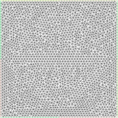
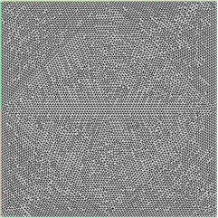
Figure 1: Example meshes. Left: 2373 vertices and 4568 triangles. Right: 8643 vertices and 16948 triangles.

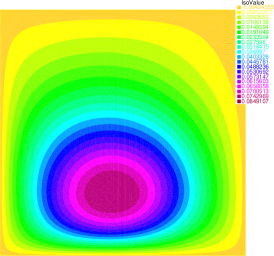
Figure 2: Left: Solution. Right: Partition into 16 subdomains for $\mathbf{H}_{\text{DD}}$

The problem is discretized by Lagrange $\mathbb{P}_{1}$ finite elements on a triangular mesh. Two example meshes are shown in Figure 1 with different levels of refinement. They are good representatives of the meshes used throughout our numerical testing. We have deliberately not chosen a regular mesh since this assumption is not required by our theory. The solution is shown in Figure 2 (left). The WPD-GMRES algorithm is implemented in Octave while the finite element matrices are assembled by FreeFem++ [16]. All iteration counts for WPD-GMRES correspond to the number of iterations needed to reach $\|\mathbf{r}_{i}\|_{\mathbf{H}}<10^{-10}\|\mathbf{b}\|_{\mathbf{H}}$ starting from a zero initial vector. The Dirichlet boundary condition has been enforced by elimination. Let $(\phi_{i})_{1\leq i\leq n}$ denote the $\mathbb{P}_{1}$ finite element basis corresponding to the mesh. The problem matrix splits into

$$\mathbf{A}=\mathbf{M}+\eta\tilde{}\mathbf{N},\text{ with }\mathbf{M}\text{ spd and }\tilde{}\mathbf{N}\text{ skew-symmetric},$$

where the entries of $\mathbf{M}$ and $\tilde{}\mathbf{N}$ are

$$\mathbf{M}_{ij}=\int_{\Omega}\left(c_{0}\phi_{i}\phi_{j}+\nu\nabla\phi_{i}\cdot\nabla\phi_{j}\right),$$

and

$$\tilde{}\mathbf{N}_{ij}=\int_{\Omega}\left(\frac{1}{2}\mathbf{\underline{a}}\cdot\nabla\phi_{i}\phi_{j}-\frac{1}{2}\mathbf{\underline{a}}\cdot\nabla\phi_{j}\phi_{i}\right),\text{ with } \mathbf{\underline{a}}(x,y)=2\pi\begin{pmatrix}0.1-y\\ x-0.5\end{pmatrix}.$$

The positive definiteness of $\mathbf{M}$ is guaranteed by the assumption that $c_{0}$ and $\nu$ are positive.

Choice of preconditioners.

For our numerical study, three preconditioners are considered:

• $\mathbf{H}=\mathbf{{I}}$ the identity matrix,

• $\mathbf{H}={{\mathbf{M}}^{-1}}$ the inverse of $\mathbf{M}$, the symmetric part of $\mathbf{A}$, and

• $\mathbf{H}=\mathbf{H}_{\text{DD}}$, a domain decomposition (DD) preconditioner based on a partition of the mesh into $N=16$ subdomains (as shown in Figure 2–Right).

The choice of $\mathbf{H}={{\mathbf{M}}^{-1}}$ was used, e.g., in [1]. It is also a fundamental feature of the CGW method [7, 26, 28], and was successfully used recently for the solution of Port-Hamiltonian systems [13].

For $\mathbf{H}=\mathbf{H}_{\text{DD}}$, The condition number of the resulting preconditioned operator is bounded by

$$\kappa(\mathbf{H}_{\text{DD}}\mathbf{M})\leq k_{0}\left(1+\frac{k_{0}}{\tau^{\prime}}\right),$$

where $k_{0}$ denotes the maximal number of subdomains that each mesh element belongs to [21, Theorem 4.40] and $\tau^{\prime}$ is a parameter that has been set to $0.15$. The constant in the bound does not depend on the total number $N$ of subdomains or the mesh parameter $h$.

In detail, $\mathbf{H}_{\text{DD}}$ is the Additive Schwarz domain decomposition method with the GenEO coarse space [23, 24]. The partition of $\Omega$ into $N$ subdomains $\Omega_{s}$ is computed automatically by Metis. One layer of overlap is added to each $\Omega_{s}$. Letting ${\mathbf{R}_{s}}^{\top}$ ($s=1,\dots,N$) denote the prolongation by zero of local finite element functions (in $\Omega_{s}$) to the whole of $\Omega$, the preconditioner can be written as

$$\mathbf{H}_{\text{DD}}=\boldsymbol{\Pi}\sum\limits_{s=1}^{N}\mathbf{R}_{s}^{\top}\underbrace{(\mathbf{R}_{s}\mathbf{M}\mathbf{R}_{s}^{\top})^{-1}}_{\text{local solves}}\mathbf{R}_{s}\boldsymbol{\Pi}^{\top}+\mathbf{R}_{0}^{\top}\underbrace{(\mathbf{R}_{0}\mathbf{M}\mathbf{R}_{0}^{\top})^{-1}}_{\text{coarse solve}}\mathbf{R}_{0},$$

where $\boldsymbol{\Pi}=\mathbf{{I}}-\mathbf{R}_{0}^{\top}(\mathbf{R}_{0}\mathbf{M}\mathbf{R}_{0}^{\top})^{-1}\mathbf{R}_{0}\mathbf{M}$ is the coarse projector (also known as a deflation operator) and the vectors in $\mathbf{R}_{0}^{\top}$ span the coarse space (or deflation space). The particularity of GenEO is that the coarse vectors are constructed by solving the low frequency eigenmodes for a generalized eigenvalue problem in each subdomain.

Deflation Operator.

We aim to illustrate the convergence result in Theorem 6. Once $\mathbf{M}$ and $\mathbf{N}$ have been assembled by FreeFem++, they are imported into Octave. The generalized eigenvalue problem (4) (i.e., $\mathbf{N}\mathbf{z}^{(j)}=\lambda_{j}\mathbf{M}\mathbf{z}^{(j)}$) is partially solved by eigs: the eigenpairs corresponding to the eigenvalues of largest magnitude are approximated. The eigenpairs are ordered in decreasing order of magnitude of $\lambda_{j}$. Since our problem is real-valued, the eigenvectors can be grouped into complex conjugate pairs and we apply the strategy from Theorem 7 to obtain real-valued deflation operators. The Octave command is $\mathbf{Z}$ = [real($\mathbf{V}$(:,1:2:m)), imag($\mathbf{V}$(:,1:2:m))], where the columns of $\mathbf{V}$ are the sorted eigenvectors and m is the (even) number of vectors that should form the deflation space. Finally, we set $\mathbf{Y}=\mathbf{H}\mathbf{A}\mathbf{Z}$ and compute the deflation operators as in Definition 1.

Remark 7.

When $\mathbf{H}=\mathbf{H}_{\text{DD}}$ is applied, the preconditioner already contains a deflation operator $\boldsymbol{\Pi}$ which corresponds to a deflation space formed by eigenvectors of frequency less than a chosen $\tau^{\prime}$ of well chosen eigenproblems in the subdomains. The presence of a deflation operator and deflation space in $\mathbf{H}_{\text{DD}}$ does not interfere with the computation of a deflation space and deflation operator following the definition in Definition 2.

Quantities of interest.

We report the number of iterations needed for WPD-GMRES to achieve convergence from a zero initial vector, with the preconditioners and deflation operators introduced above, and the weight matrix $\mathbf{W}=\mathbf{H}$. The stopping criterion is $\|\mathbf{r}_{i}\|_{\mathbf{H}}<10^{-10}\|\mathbf{b}\|_{\mathbf{H}}$. We also report the upper bound for $\theta$ predicted by Theorem 6 (case 1) as well as the corresponding experimental value

$$\theta_{th}=\frac{1}{\kappa(\mathbf{H}\mathbf{M})}\times\frac{1}{{1+|\lambda_{m+1}|^{2}}}\text{ and }\theta_{exp}=\min\limits_{i}\left\{1-\frac{\|\mathbf{r}_{i+1}\|_{\mathbf{H}}^{2}}{\|\mathbf{r}_{i}\|_{\mathbf{H}}^{2}}\right\}.$$

The threshold $\tau$ in the theoretical bound has been substituted for $|\lambda_{m+1}|$, the modulus of the largest eigenvalue not used for the deflation space. In order to compute $\theta_{th}$, $\kappa(\mathbf{H}\mathbf{M})$ is approximated by solving a linear system for matrix $\mathbf{M}$ preconditioned by $\mathbf{H}$ with PCG and taking the ratio of the Ritz values. The theorem guarantees that $\theta_{th}\leq\theta_{exp}$ and this has indeed been the case for every single one of our numerical experiments.

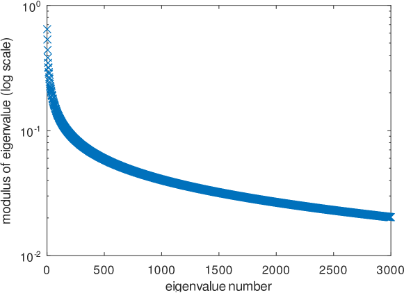
Figure 3: $|\lambda_{1}|$ to $|\lambda_{3000}|$ in log scale (solution of (4))

m	0	10	50	100	200	500	1000
$|\lambda_{\text{m}+1}|$	0.65	0.32	0.18	0.13	0.09	0.06	0.04
$\theta_{th}$ for $\mathbf{H}={{\mathbf{M}}^{-1}}$	0.71	0.91	0.97	0.98	0.991	0.997	0.998
$\theta_{th}$ for $\mathbf{H}=\mathbf{H}_{\text{DD}}$	0.043	0.056	0.0597	0.0605	0.0610	0.0614	0.0615
$\theta_{th}$ for $\mathbf{H}=\mathbf{{I}}$	7.1e-05	9.2e-05	9.8e-05	9.9e-05	1.001e-04	1.007e-04	1.009e-04

Table 1: If m is the rank of the deflation space, the second line is the modulus of the first eigenvalue not included in the deflation space, and the next three lines correspond to the theoretical bound $\theta_{th}$ for out three choices of preconditioner.

Results for $\eta=1$.

For this test case, we use a mesh with 63658 triangles and 32158 vertices. Once the homogeneous Dirichlet boundary condition has been treated by elimination, the problem has 31502 degrees of freedom. The parameter in the convection field is $\eta=1$ so that $\mathbf{A}=\mathbf{M}+\mathbf{N}$, with $\mathbf{N}=\tilde{}\mathbf{N}$. We first solve generalized eigenproblem (4). The spectrum is represented in Figure 3 where the magnitudes of the 3000 largest (purely imaginary) eigenvalues are represented. It is slightly disappointing that the distribution of eigenvalues does not consist in a cluster of large eigenvalues and a tail of eigenvalues tightly clustered around 0. This would indeed have been ideal for selecting a value of $\tau$ to compute the deflation space with the formula in Definition 2. Table 1 gives the value of $|\lambda_{\text{m}+1}|$ for a few choices of m as well as the resulting bounds for $\theta$. In these bounds we have injected the approximate condition number $\kappa(\mathbf{H}\mathbf{M})$ which takes the following values

$$\kappa(\mathbf{{I}}\mathbf{M})=9896.4,\quad\kappa(\mathbf{H}_{\text{DD}}\mathbf{M})=16.241,\quad\text{and }\kappa({{\mathbf{M}}^{-1}}\mathbf{M})=1.$$

We now solve the problem with all three preconditioners and varying ranks m of the deflation spaces. The case $\text{m}=0$ corresponds to weighted and preconditioned GMRES with no deflation. The largest deflation space has rank $1000$ which corresponds to 3.2% of the total number of degrees of freedom (dofs). The convergence curves are shown in Figure 4. We observe that our choice of deflation space indeed improves convergence: when the deflation space gets larger, the number of iterations is reduced. Since the case is only mildly nonsymmetric ($\rho(\mathbf{M}^{-1}\mathbf{N})=0.65$), the two good preconditioners for $\mathbf{M}$ also give good results for the full problem even with $\text{m}=0$. For $\mathbf{H}=\mathbf{{I}}$, though, the effect of deflation is welcome: deflating $10$ vectors reduces the iteration count from 671 to 543 and deflating 50 vectors reduces the iteration count from 671 to 440.

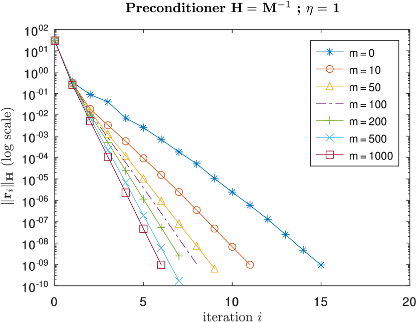
m	iter	$\theta_{th}$	$\theta_{exp}$
0	15	7.059e-01	7.956e-01
10	11	9.071e-01	9.685e-01
50	9	9.697e-01	9.912e-01
100	8	9.835e-01	9.951e-01
200	7	9.914e-01	9.975e-01
500	7	9.965e-01	9.990e-01
1000	6	9.984e-01	9.995e-01

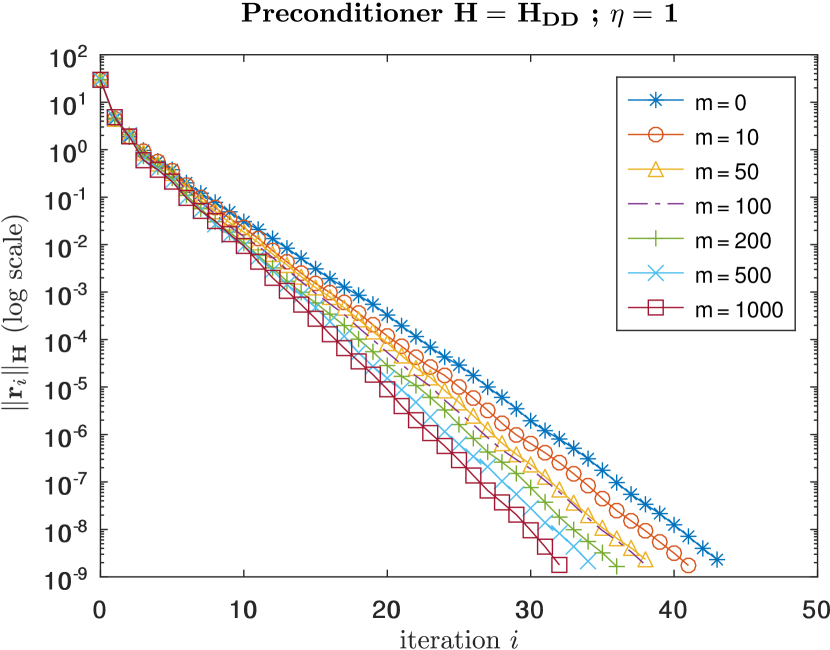
m	iter	$\theta_{th}$	$\theta_{exp}$
0	43	4.346e-02	5.314e-01
10	41	5.585e-02	5.539e-01
50	38	5.970e-02	5.977e-01
100	38	6.055e-02	5.978e-01
200	36	6.104e-02	5.834e-01
500	34	6.136e-02	6.183e-01
1000	32	6.147e-02	6.017e-01

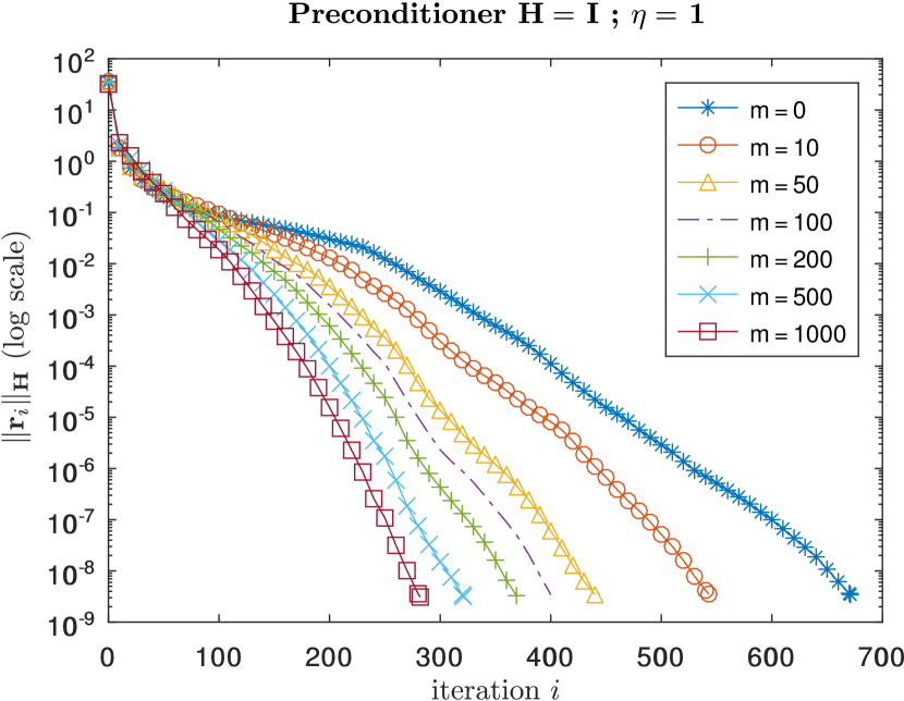
m	iter	$\theta_{th}$	$\theta_{exp}$
0	671	7.133e-05	1.658e-02
10	543	9.166e-05	2.998e-02
50	440	9.798e-05	4.152e-02
100	400	9.938e-05	4.772e-02
200	369	1.002e-04	5.229e-02
500	321	1.007e-04	6.847e-02
1000	282	1.009e-04	8.047e-02

Figure 4: Convergence curves when $\eta=1$ with varying preconditioner and rank of deflation space

Results for $\eta=100$.

Next we change the value of $\eta$ to $100$. The global matrix is now $\mathbf{A}=\mathbf{M}+\mathbf{N}$ with $\mathbf{N}=100\tilde{}\mathbf{N}$, and the problem is much more nonsymmetric. The eigenvalues arising from (4) get multiplied by $100$ which has the effect of seriously deteriorating the bounds for $\theta$. Figure 5 shows the convergence curves in this case. Again, we confirm that applying a preconditioner tailored for the symmetric part is a good idea (with 341 or 352 iterations instead of 1276). In the non-preconditioned case, it occurs that the non-deflated problem converges the fastest. This is surprising but does not contradict the theory. Figure 6 shows the first 1000 residuals in this case for m$=0$ and m$=100$. It can be observed that deflation initially accelerates convergence, particularly where it is slowest. However, after roughly 500 iterations, the non-deflated algorithm is faster. For $\mathbf{H}=\mathbf{H}_{\text{DD}}$ or ${{\mathbf{M}}^{-1}}$, convergence improves when more vectors are added to the deflation space. With $\mathbf{H}={{\mathbf{M}}^{-1}}$, deflating 10 vectors reduces the iteration count from 341 to 331 and deflating 100 vectors reduces it further to 259. With $\mathbf{H}=\mathbf{H}_{\text{DD}}$, deflating 10 vectors reduces the iteration count from 352 to 343 and deflating 100 vectors reduces it further to 275.

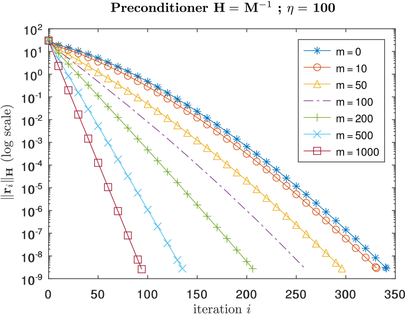
m	iter	$\theta_{th}$	$\theta_{exp}$
0	341	2.399e-04	3.144e-03
10	331	9.756e-04	4.517e-02
50	296	3.186e-03	8.368e-02
100	259	5.918e-03	1.040e-01
200	206	1.139e-02	1.376e-01
500	135	2.796e-02	2.101e-01
1000	94	5.767e-02	2.943e-01

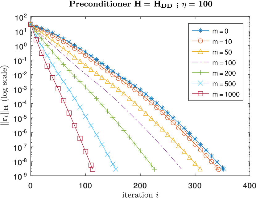
m	iter	$\theta_{th}$	$\theta_{exp}$
0	352	1.477e-05	7.453e-03
10	343	6.007e-05	1.794e-02
50	309	1.962e-04	4.418e-02
100	275	3.644e-04	6.712e-02
200	226	7.016e-04	1.029e-01
500	155	1.721e-03	1.947e-01
1000	113	3.551e-03	2.901e-01

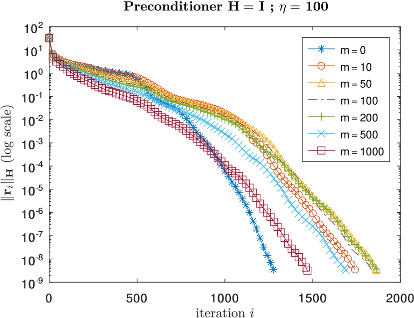
m	iter	$\theta_{th}$	$\theta_{exp}$
0	1276	2.424e-08	4.447e-03
10	1740	9.858e-08	3.898e-03
50	1863	3.219e-07	4.036e-03
100	1835	5.980e-07	4.058e-03
200	1865	1.151e-06	5.914e-03
500	1688	2.825e-06	7.266e-03
1000	1470	5.828e-06	9.225e-03

Figure 5: Convergence curves when $\eta=100$ with varying preconditioner and rank of deflation space

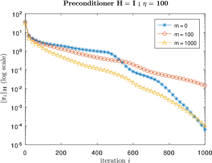
Figure 6: Zoom on the first 1000 iterations in the case $\mathbf{H}=\mathbf{{I}}$ and $\eta=100$.

Influence of the mesh.

We consider the case where $\eta=100$ and $\mathbf{H}=\mathbf{H}_{\text{DD}}$ with varying mesh size. The stopping criterion is as before, $\|\mathbf{r}_{i}\|_{\mathbf{H}}/\|\mathbf{r}_{0}\|_{\mathbf{H}}=\|\mathbf{r}_{i}\|_{\mathbf{H}}/\|\mathbf{b}\|_{\mathbf{H}}<10^{-10}$. The three considered meshes are the $32158$ vertex mesh that was used in the tests above as well as the two less refined meshes represented in Figure 1 (2373 and 8643 vertices). After elimination of the degrees of freedom on the boundary, the resulting linear systems have respectively 31502, 8307 and 2197 dofs. The problem is solved by WPD-GMRES without deflation ($\text{m}=0$ and with deflation of $\text{m}=100$ vectors). The results are presented in Table 2. We notice that the iteration counts increase weakly with the mesh size. For example, from 236 for 2,197 dofs to 275 for 32,502 dofs in the case where 100 vectors are deflated. We also report on the quantities that appear in the convergence bounds: $\kappa(\mathbf{H}_{\text{DD}}\mathbf{M})$, $|\lambda_{1}|=\rho(\mathbf{M}^{-1}\mathbf{N})$ and $|\lambda_{101}|$. We know from the theory in [24] that $\kappa(\mathbf{H}_{\text{DD}}\mathbf{M})$ is bounded independently of the mesh size and we indeed notice that it does not depend very much on the mesh. In [22, Section 5], it was proved that for this particular PDE, $|\lambda_{1}|=\rho(\mathbf{M}^{-1}\mathbf{N})$ is also bounded independently of the mesh size by

$$\rho(\mathbf{M}(\mathbf{A})^{-1}\mathbf{N}(\mathbf{A}))\leq\frac{1}{2}\frac{\|\mathbf{a}\|_{L^{\infty}(\Omega)}}{\sqrt{\inf(\nu)\inf(c_{0}+\frac{1}{2}\operatorname{div}(\mathbf{a}))}}=3.23\eta=323.$$ (11)

The bound is satisfied here and $\rho(\mathbf{M}^{-1}\mathbf{N})$ does not depend on the mesh. For $|\lambda_{101}|$, we have no theoretical results (except of course that $|\lambda_{101}|\leq\rho(\mathbf{M}(\mathbf{A})^{-1}\mathbf{N}(\mathbf{A}))$) and we observe a small increase when the number of dofs increases.

$\#$ dofs	Iter		$\kappa(\mathbf{H}_{\text{DD}}\mathbf{M})$	$|\lambda_{1}|=\rho(\mathbf{M}^{-1}\mathbf{N})$	$|\lambda_{101}|$
	$\text{m}=0$	$\text{m}=100$
2,197	316	236	14.4	64.4	11.5
8,307	343	267	14.2	64.5	12.7
32,502	352	275	13.0	64.6	13.0

Table 2: For $\eta=100$ and $\mathbf{H}=\mathbf{H}_{\text{DD}}$, three mesh sizes are considered

Comparison with left preconditioned and deflated GMRES.

As a final test we examine whether GMRES with the same preconditioner (applied on the left) and deflation operator but without the change of inner product exhibits the same convergence behavior as WPD-GMRES (i.e., preconditioned and deflated GMRES in the $\mathbf{H}$-inner product). To this end we solve the same problem twice: once with WPD-GMRES and once with preconditioned and deflated GMRES. In both cases the stopping criterion is set to $\|\mathbf{H}\mathbf{r}_{i}\|/\|\mathbf{H}\mathbf{r}_{0}\|=\|\mathbf{H}\mathbf{r}_{i}\|/\|\mathbf{H}\mathbf{b}\|<10^{-10}$ where $\|\cdot\|$ is the Euclidean norm. As an illustration, we choose the problem with 8,307 dofs and set $\mathbf{H}=\mathbf{H}_{\text{DD}}$. Problems with ($\eta\in\{0.1,1,10,100\}$) are solved without deflation and with deflation of $100$ vectors. The iteration counts can be found in Table 3. The fact that the number of iterations is nearly identical in the weighted and unweighted cases is remarkable. The iteration count for the unweighted method is always the smallest. This is due to the fact that the chosen stopping criterion is precisely the norm that is minimized by the unweighted method. In Figure 7 we plot the history of residual $\|\mathbf{H}\mathbf{r}_{i}\|/\|\mathbf{H}\mathbf{r}_{0}\|$ for $\eta=100$. Again, we observe a strong similarity and the minimization property of GMRES ensures that in this norm, the residual for $\mathbf{W}=\mathbf{{I}}$ will always be below the residual for $\mathbf{W}=\mathbf{H}$.

$\eta$	$\text{m}=0$		$\text{m}=100$
	$\mathbf{W}=\mathbf{{I}}$	$\mathbf{W}$= $\mathbf{H}$	$\mathbf{W}=\mathbf{{I}}$	$\mathbf{W}$= $\mathbf{H}$
0.1	36	37	33	33
1	40	40	33	34
10	89	90	54	54
100	327	329	253	255

Table 3: Iteration counts for weighted and unweighted algorithms. Both algorithms use the stopping criterion coming from the unweighted algorithm

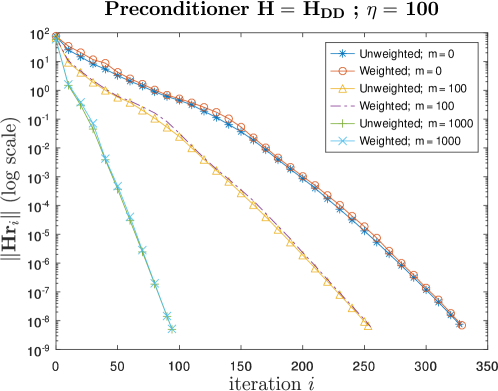
Figure 7: Comparison of weighted and unweighted algorithms, without deflation and with deflation of $100$ vectors. The chosen norm is the one that is minimized by the unweighted algorithm

9 Conclusions

We present a very general convergence bound for preconditioned GMRES when any inner product is used, and when it is deflated. We consider bounds for several generic cases for the deflation space. These bounds inspired us to produce an effective deflation space, namely, the eigenvectors of the generalized eigenvalue problem $\mathbf{N}\mathbf{z}=\lambda\mathbf{M}\mathbf{z}$, where $\mathbf{M}$ is the Hermitian part of $\mathbf{A}$, which is assumed to be positive definite, and $\mathbf{N}$ is the skew-Hermitian part of $\mathbf{A}$. Only eigenvectors corresponding to eigenvalues with muduli above a given threshold are selected. Numerical experiments illustrate the potential for these ideas. Deflating indeed reduces the number of iterations, and so do the preconditioners combined with the deflation. On the other hand, while our theory applies to any inner product, our experiments do not show an improvement with our choices of the weights.

References

- [1] Z. Bai, J. Yin, and Y. Su. A shift-splitting preconditioner for non-Hermitian positive definite matrices. J. Comput. Math., 24:539–552, 2006.
- [2] M. Benzi. Preconditioning techniques for large linear systems: A survey. J. Comp. Phys., 182:418–477, 2002.
- [3] P. N. Brown and H. F. Walker. GMRES on (nearly) singular systems. SIAM J. Matrix Anal. Appl., 18:37–51, 1997.
- [4] K. Burrage, J. Erhel, B. Pohl, and A. Williams. A deflation technique for linear systems of equations. SIAM J. Sci. Comput., 19:1245–1260, 1998.
- [5] T. F. Chan, E. Chow, Y. Saad, and M. C. Yeung. Preserving symmetry in preconditioned Krylov subspace methods. SIAM J. Sci. Comput., 20:568–581, 1999.
- [6] A. Chapman and Y. Saad. Deflated and augmented Krylov subspace techniques. Numer. Linear Algebra Appl., 4:43–66, 1997.
- [7] P. Concus and G. H. Golub. A generalized conjugate gradient method for nonsymmetric systems of linear equations. In R. Glowinski and J.-L. Lions, editors, Computing methods in applied sciences and engineering (Second Internat. Sympos., Versailles, 1975), Part 1, volume 134 of Lecture Notes in Econom. and Math. Systems, pages 56–65. Springer, Berlin, 1976.
- [8] M. Embree, R. B. Morgan, and H. V. Nguyen. Weighted inner products for GMRES and GMRES-DR. SIAM J. Sci. Comput., 39:S610–S632, 2017.
- [9] Y. A. Erlangga and R. Nabben. Deflation and balancing preconditioners for Krylov subspace methods applied to nonsymmetric matrices. SIAM J. Matrix Anal. Appl., 30:684–699, 2008.
- [10] A. Essai. Weighted FOM and GMRES for solving nonsymmetric linear systems. Numer. Algorithms, 18:277–292, 1998.
- [11] L. García Ramos, R. Kehl, and R. Nabben. Projections, deflation, and multigrid for nonsymmetric matrices. SIAM J. Matrix Anal. Appl., 41:83–105, 2020.
- [12] A. Gaul, M. H. Gutknecht, J. Liesen, and R. Nabben. A framework for deflated and augmented Krylov subspace methods. SIAM J. Matrix Anal. Appl., 34:495–518, 2013.
- [13] C. Güdücü, J. Liesen, V. Mehrmann, and D. B. Szyld. On non-Hermitian positive (semi)definite linear algebraic systems arising from dissipative Hamiltonian DAEs. SIAM J. Sci. Computing, 44:A2871–A2894, 2022.
- [14] S. Güttel and J. Pestana. Some observations on weighted GMRES. Numer. Algorithms, 67:733–752, 2014.
- [15] K. Hayami and M. Sugihara. A geometric view of Krylov subspace methods on singular systems. Numer. Linear Algebra Appl., 18:449–469, 2011.
- [16] F. Hecht. New development in FreeFem++. J. Numer. Math., 20(3-4):251–265, 2012.
- [17] R. A. Horn and C. R. Johnson. Matrix Analysis. Cambridge University Press, Cambridge, 1985.
- [18] Y. Saad. Iterative methods for sparse linear systems. Philadelphia, PA: SIAM Society for Industrial and Applied Mathematics, 2nd ed. edition, 2003.
- [19] Y. Saad and M. H. Schultz. GMRES: A generalized minimal residual algorithm for solving nonsymmetric linear systems. SIAM J. Sci. Stat. Comput., 7:856–869, 1986.
- [20] V. Simoncini and D. B. Szyld. Recent computational developments in Krylov subspace methods for linear systems. Numer. Linear Algebra Appl., 14:1–59, 2007.
- [21] N. Spillane. Robust domain decomposition methods for symmetric positive definite problems. PhD thesis, UPMC, 2014.
-
[22]
N. Spillane.
Hermitian preconditioning for a class of non-Hermitian linear
systems, 2023.
Available at the arXiv:2304.03546, and also at
https://hal.science/hal-04028590. To appear in SIAM J. Sci. Stat. Comput. - [23] N. Spillane, V. Dolean, P. Hauret, F. Nataf, C. Pechstein, and R. Scheichl. A robust two-level domain decomposition preconditioner for systems of PDEs. C. R. Math. Acad. Sci. Paris, 349(23-24):1255–1259, 2011.
- [24] N. Spillane, V. Dolean, P. Hauret, F. Nataf, C. Pechstein, and R. Scheichl. Abstract robust coarse spaces for systems of PDEs via generalized eigenproblems in the overlaps. Numer. Math., 126(4):741–770, 2014.
- [25] G. Starke. Field-of-values analysis of preconditioned iterative methods for nonsymmetric elliptic problems. Numer. Math., 78:103–117, 1997.
- [26] D. B. Szyld and O. B. Widlund. Variational analysis of some conjugate gradient methods. East-West J. Numer. Math., 1:51–74, 1993.
- [27] J. M. Tang, R. Nabben, C. Vuik, and Y. A. Erlangga. Comparison of two-level preconditioners derived from deflation, domain decomposition and multigrid methods. J. Sci. Comput., 39:340–370, 2009.
- [28] O. Widlund. A Lanczos method for a class of nonsymmetric systems of linear equations. SIAM J. Numer. Anal., 15:801–812, 1978.