Generalized system-bath entanglement theorem for Gaussian environments

Abstract

A system-bath entanglement theorem (SBET) with Gaussian environments was established previously in J. Chem. Phys. 152, 034102 (2020) in terms of linear response functions. This theorem connects the system-bath entanglement responses to the local system and bare bath ones. In this work, we generalize it to correlation functions. Key steps in derivation are the generalized Langevin dynamics for the hybridizing bath modes as in the previous work, together with the Bogoliubov transformation mapping the original finite-temperature canonical reservoir to an effective zero-temperature vacuum via an auxiliary bath. With the theorem, the system-bath entangled correlations and the bath modes correlations in the full composite space can be evaluated as long as the bare-bath statistical properties are known and the reduced system correlations are obtained. Numerical demonstrations are carried out for the evaluation of the solvation free energy of an electron transfer system with a certain intramolecular vibrational modes.

I Introduction

Many fields of modern research inevitably encounter the system–plus–environments hybridized effects which can be crucial.[1] Various developments of quantum dissipation methods are mainly based on Gaussian properties of environments (thermal baths) being composed of non-interacting harmonic oscillators coupled linearly to the system.[2, 3] Methods cover from perturbative master equation approaches,[4, 5, 6, 7, 8] stochastic approaches,[9, 10, 11, 12, 13, 14, 15, 16] the multilayer multiconfiguration time-dependent Hartree method (ML-MCTDH),[17] to Feynman–Vernon influence functional path integral[18] and its executable propagators,[19, 20, 21] together with its differential equivalence, the hierarchical–equations–of–motion (HEOM) formalism.[22, 23, 24, 25]

Most of these methods primarily focus on the reduced system dynamics under the influence of thermal environments. On the other hand, the system-bath entanglement can take essential effect in, for example, Fano resonances,[26, 27, 28] vibronic spectroscopies,[29] and thermal transports.[30] To this end, a dissipaton equation of motion (DEOM) approach has been systematically developed in recent years, as an exact, quasi-particle theory for system–environment hybridized dynamics.[31, 32, 33, 34] For the dynamics of the reduced system, the DEOM recovers the HEOM.

A system-bath entanglement theorem (SBET) for Gaussian environments was established in our previous work.[35] This theorem connects the entangled system-bath linear response functions in the total system–plus–bath space to the local responses of associated system variables and the bath responses of the hybridizing modes in the bare–bath space. Thus the theorem enables those quantum dissipation methods which only evaluate the system responses to obtain the system-bath entangled properties as well.

The SBET[35] was constructed independent of concrete ensembles. The key step in establishing it is the generalized Langevin dynamics for the hybridizing bath modes. It leads to the SBET existing for any steady state of the composites. On the other hand, due to the less information of response functions with respect to correlation functions, it would be inconvenient to further derive the relation between correlations from the original SBET.[35]

In this work, we establish a generalized SBET for the connection of correlation functions among system-bath entangled, local system, and bare bath ones. It is achieved via the Bogoliubov transformation[36] mapping the original finite-temperature canonical reservoir to an effective zero-temperature vacuum by adding an auxiliary bath. The original SBET[35] can be recovered straightforwardly from the generalized one here. Like the original one, the generalized SBET here is also established for steady states. It is shown to satisfy the detailed–balance relation in the condition of the canonical ensemble thermal equilibrium. The evaluation on expectation values of entangled system-bath properties would just be the special case of correlation functions.

For numerical demonstrations we apply the theorem to evaluate the solvation free energy of an electron transfer (ET) system involved with several intramolecular vibrational normal modes and embedded into a Gaussian solvent. Particularly, based on the generalized SBET, a multi-scale approach is provided to investigate the solvation effects. The SBET connects different dynamical scales in a rigorous way, preserving all the important information such as environmental memory and cross–scale correlations. As a result, in order to obtain the hybridization free energy for the mixing between solvent and solute molecule which includes both electronic and nuclear degrees of freedom, we only need to carry out the calculation on the electronic subsystem. This largely reduces computing cost. The rest of paper is organized as follows. The generalized SBET is constructed in Sec. II with more derivation details given in Appendix A and the detailed–balance proof for the canonical ensemble given in Appendix B. Numerical demonstrations are presented and discussed in Sec. III. The paper is finally summarized in Sec. IV.

II Generalized system-bath entanglement theorem

II.1 Prelude

Let us start with the total system–plus–bath composite Hamiltonian reading[35]

$$H_{\mbox{\tiny T}}=H_{\mbox{\tiny S}}+h_{\mbox{\tiny B}}+H_{\mbox{\tiny SB}}\equiv H_{\mbox{\tiny S}}+h_{\mbox{\tiny B}}+\sum_{u}\hat{Q}_{u}\hat{F}_{u}.$$ (1)

Here, the system Hamiltonian $H_{\mbox{\tiny S}}$ and dimensionless dissipative modes $\{\hat{Q}_{u}\}$ are arbitrary and Hermitian. The Gaussian environment scenario requires

$$h_{\mbox{\tiny B}}=\sum_{j}\hbar\omega_{j}\hat{a}_{j}^{\dagger}\hat{a}_{j}\quad\text{and}\quad\hat{F}_{u}=\frac{1}{\sqrt{2}}\sum_{j}\hbar c_{uj}(\hat{a}_{j}^{\dagger}+\hat{a}_{j}),$$ (2)

where $\{\hat{a}^{\dagger}_{j}\}$ and $\{\hat{a}_{j}\}$ are the creation and annihilation operators of bath oscillators. For the generalized SBET to be established, we consider the averages of variables under the following steady state

$$\rho_{\rm st}\equiv\lim_{t_{0}\to-\infty}e^{iH_{\mbox{\tiny T}}t_{0}/\hbar}\rho_{\mbox{\tiny T}}(t_{0})e^{-iH_{\mbox{\tiny T}}t_{0}/\hbar},$$ (3)

satisfying $[H_{\mbox{\tiny T}},\rho_{\rm st}]=0$. The total composites are initialized at $t_{0}$ with

$$\rho_{\mbox{\tiny T}}(t_{0})=\rho_{\mbox{\tiny S}}(t_{0})\rho_{\mbox{\tiny B}}^{\rm eq}\equiv\rho_{\mbox{\tiny S}}(t_{0})e^{-\beta h_{\mbox{\tiny B}}}/{\rm tr}_{\mbox{\tiny B}}e^{-\beta h_{\mbox{\tiny B}}}.$$ (4)

Here $\beta=1/(k_{B}T)$ with $k_{B}$ being the Boltzmann constant and $T$ the temperature. Correspondingly, denote operators in Heisenberg picture by

$$\hat{O}(t)\equiv e^{iH_{\mbox{\tiny T}}(t-t_{0})/\hbar}\hat{O}e^{-iH_{\mbox{\tiny T}}(t-t_{0})/\hbar},$$ (5)

and the correlation functions

$$\langle\hat{A}(t) \hat{B}(0)\rangle\equiv{\rm Tr}\big{(}e^{iH_{\mbox{\tiny T}}t/\hbar}\hat{A}e^{-iH_{\mbox{\tiny T}}t/\hbar}\hat{B}\rho_{\rm st}\big{)}$$

$$=\lim_{t_{0}\to-\infty}{\rm Tr}\big{[}e^{iH_{\mbox{\tiny T}}(t-t_{0})/\hbar}\hat{A}e^{-iH_{\mbox{\tiny T}}(t-t_{0})/\hbar}$$

$$\qquad\qquad\quad\times e^{-iH_{\mbox{\tiny T}}t_{0}/\hbar}\hat{B}e^{iH_{\mbox{\tiny T}}t_{0}/\hbar}\rho_{\mbox{\tiny T}}(t_{0})\big{]}$$

$$=\langle\hat{B}(-t)\hat{A}(0)\rangle^{\ast},$$ (6)

where $\hat{A}$ and $\hat{B}$ are Hermitian operators. The second equality shows the equivalence between the $\rho_{0}$ and $\rho_{\rm st}$ descriptions for correlation functions.

The Gaussian bath property is fully characterized via its bare–bath correlation function, namely,

$$c_{uv}(t)\equiv\langle\hat{F}^{\mbox{\tiny B}}_{u}(t)\hat{F}^{\mbox{\tiny B}}_{v}(0)\rangle_{\mbox{\tiny B}}=c^{\ast}_{vu}(-t)$$ (7)

where $\hat{F}^{\mbox{\tiny B}}_{u}(t)\equiv e^{ih_{\mbox{\tiny B}}(t-t_{0})/\hbar}\hat{F}_{u}e^{-ih_{\mbox{\tiny B}}(t-t_{0})/\hbar}$ and $\langle(\cdots)\rangle_{\mbox{\tiny B}}\equiv{\rm tr}_{\mbox{\tiny B}}[(\cdots)\rho^{\rm eq}_{\mbox{\tiny B}}]$ with $\rho^{\rm eq}_{\mbox{\tiny B}}\equiv e^{-\beta h_{\mbox{\tiny B}}}/{\rm Tr}(e^{-\beta h_{\mbox{\tiny B}}})\equiv e^{-\beta h_{\mbox{\tiny B}}}/Z_{\mbox{\tiny B}}$. The fluctuation–dissipation theorem (FDT) gives[1]

$$c_{uv}(t)=\frac{\hbar}{\pi}\int_{-\infty}^{\infty}\!\!{\mathrm{d}}\omega\,e^{-i\omega t}\frac{J_{uv}(\omega)}{1-e^{-\beta\hbar\omega}},$$ (8)

with the interacting bath spectral density being

$$J_{uv}(\omega)\equiv\frac{1}{2i}\int_{-\infty}^{\infty}\!\!{\mathrm{d}}t\,e^{i\omega t}\phi_{uv}(t)$$ (9)

and the bare–bath response function

$$\phi_{uv}(t)\equiv\frac{i}{\hbar}\langle[\hat{F}^{\mbox{\tiny B}}_{u}(t),\hat{F}^{\mbox{\tiny B}}_{v}(0)]\rangle_{\mbox{\tiny B}}=-\frac{2}{\hbar}{\rm Im}[c_{uv}(t)].$$ (10)

For the Gaussian bath scenario, Eq. (2), we can easily obtain

$${\phi}_{uv}(t)=\hbar\sum_{j}c_{uj}c_{vj}\sin(\omega_{j}t),$$ (11)

$$J_{uv}(\omega)=\frac{\pi}{2}\hbar\sum_{j}c_{uj}c_{vj}[\delta(\omega-\omega_{j})-\delta(\omega+\omega_{j})],$$ (12)

and

$$c_{uv}(t)=\frac{\hbar^{2}}{2}\sum_{j}c_{uj}c_{vj}\left[\bar{n}_{j}e^{i\omega_{j}t}+(\bar{n}_{j}+1)e^{-i\omega_{j}t}\right],$$ (13)

with $\bar{n}_{j}\equiv(e^{\beta\hbar\omega_{j}}-1)^{-1}$ the average occupation number. For later use, we define

$$c^{-}_{uv}(t)\equiv c_{uv}(t)\quad{\rm and}\quad c^{+}_{uv}(t)\equiv[c^{-}_{uv}(t)]^{\ast}.$$ (14)

II.2 Thermofield decomposition and Langevin dynamics

For the convenient derivation to obtain the SBET in terms of correlation functions defined in Eq. (II.1), we can apply the Bogoliubov transformation[36] by adding an auxiliary bath $h_{\mbox{\tiny B}}^{\prime}=-\sum_{j}\hbar\omega_{j}\hat{a}_{j}^{\prime\dagger}\hat{a}^{\prime}_{j}$ to purify $\rho_{\mbox{\tiny B}}^{\rm eq}$ into a vacuum state of the effective bath, $\tilde{h}_{\mbox{\tiny B}}\equiv h_{\mbox{\tiny B}}+h_{\mbox{\tiny B}}^{\prime}$. Details are given in Appendix A. After the Bogoliubov transformation, let us adopt the thermofield decomposition,[36]

$$\hat{F}_{u}=\hat{F}^{+}_{u}+\hat{F}^{-}_{u},$$ (15)

with

$$\hat{F}^{-}_{u}=\frac{1}{\sqrt{2}}\sum_{j}\hbar{c_{uj}}\big{(}\sqrt{\bar{n}_{j}}\hat{d}_{j}+\sqrt{\bar{n}_{j}+1}\hat{d}^{\prime}_{j}\big{)}$$ (16)

and $\hat{F}^{+}_{u}=(\hat{F}^{-}_{u})^{\dagger}$. Here, $\hat{d}_{j}\equiv\sqrt{\bar{n}_{j}+1}\hat{a}^{\prime}_{j}-\sqrt{\bar{n}_{j}}\hat{a}^{\dagger}_{j}$ and $\hat{d}^{\prime}_{j}\equiv\sqrt{\bar{n}_{j}+1}\hat{a}_{j}-\sqrt{\bar{n}_{j}}\hat{a}^{\prime\dagger}_{j}$, as defined in Eq. (57).

For the effective total Hamiltonian, $\widetilde{H}_{\mbox{\tiny T}}=H_{\mbox{\tiny S}}+\tilde{h}_{\mbox{\tiny B}}+\sum_{u}\hat{Q}_{u}\hat{F}_{u}$, the Heisenberg equation of motion gives $\dot{\hat{a}}^{\prime}_{j}(t)=i\omega_{j}\hat{a}^{\prime}_{j}(t)$, $\dot{\hat{a}}^{\prime\dagger}_{j}(t)=-i\omega_{j}\hat{a}^{\prime\dagger}_{j}(t)$, and

$$\dot{\hat{a}}^{\dagger}_{j}(t) =i\omega_{j}\hat{a}_{j}^{\dagger}(t)+\frac{i}{\sqrt{2}}\sum_{v}{c_{vj}}\hat{Q}_{v}(t),$$ (17a)

$$\dot{\hat{a}}_{j}(t) =-i\omega_{j}\hat{a}_{j}(t)-\frac{i}{\sqrt{2}}\sum_{v}{c_{vj}}\hat{Q}_{v}(t).$$ (17b)

The formal solutions to the above equations are ${\hat{a}}^{\prime}_{j}(t)=e^{i\omega_{j}(t-t_{0})}{\hat{a}}^{\prime}_{j}$, ${\hat{a}}^{\prime\dagger}_{j}(t)=e^{-i\omega_{j}(t-t_{0})}{\hat{a}}^{\prime\dagger}_{j}$, and

$$\hat{a}^{\dagger}_{j}(t) =e^{i\omega_{j}(t-t_{0})}\hat{a}^{\dagger}_{j}+\frac{i}{\sqrt{2}}\sum_{v}{c_{vj}}\int_{t_{0}}^{t}\!\!{\rm d}\tau\,e^{i\omega_{j}(t-\tau)}\hat{Q}_{v}(\tau),$$ (18a)

$$\hat{a}_{j}(t) =e^{-i\omega_{j}(t-t_{0})}\hat{a}_{j}-\frac{i}{\sqrt{2}}\sum_{v}{c_{vj}}\int_{t_{0}}^{t}\!\!{\rm d}\tau\,e^{-i\omega_{j}(t-\tau)}\hat{Q}_{v}(\tau).$$ (18b)

Therefore we can obtain

$$\hat{F}_{u}^{\pm}(t)=\hat{F}^{\pm;\mbox{\tiny B}}_{u}(t)\pm\frac{i}{\hbar}\sum_{v}\int_{t_{0}}^{t}\!{\mathrm{d}}\tau\,c^{\pm}_{uv}(t-\tau)\hat{Q}_{v}(\tau),$$ (19)

with

$$\hat{F}^{\pm;\mbox{\tiny B}}_{u}(t)\equiv e^{i\tilde{h}_{\mbox{\tiny B}}(t-t_{0})/\hbar}\hat{F}^{\pm}_{u}e^{-i\tilde{h}_{\mbox{\tiny B}}(t-t_{0})/\hbar}\,.$$ (20)

Apparently, $\hat{F}^{+}_{u}(t)=[\hat{F}^{-}_{u}(t)]^{\dagger}$. It is easy to verify that Eqs. (15) and (19) lead to

$$\hat{F}_{u}(t)=\hat{F}^{\mbox{\tiny B}}_{u}(t)-\sum_{v}\int_{t_{0}}^{t}\!\!{\rm d}\tau\,\phi_{uv}(t-\tau)\hat{Q}_{v}(\tau).$$ (21)

This is just the Eq.(7) in Ref. 35, i.e. the equation of Langevin dynamics for the hybridizing bath modes, which serves as the starting point to the establishment of SBET.

II.3 Derivation to the generalized SBET

We are now ready to derive the SBET for correlation functions. By Eq. (62), the second identity of Eq. (II.1) can now be recast as

$$\langle\hat{A}(t)\hat{B}(0)\rangle=\lim_{t_{0}\to-\infty}{\widetilde{\rm Tr}}\big{[} e^{i\widetilde{H}_{\mbox{\tiny T}}(t-t_{0})/\hbar}\hat{A}e^{-i\widetilde{H}_{\mbox{\tiny T}}(t-t_{0})/\hbar}$$

$$\times e^{-i\widetilde{H}_{\mbox{\tiny T}}t_{0}/\hbar}\hat{B}e^{i\widetilde{H}_{\mbox{\tiny T}}t_{0}/\hbar}\rho_{\mbox{\tiny S}}(t_{0})|\xi\rangle\langle\xi|\big{]}.$$ (22)

Here, $\widetilde{\rm Tr}(\cdots)={\rm Tr}[{\rm tr}_{\mbox{\tiny B}}^{\prime}(\cdots)]$ is the trace over the entire space of $\widetilde{H}_{\mbox{\tiny T}}=H_{\mbox{\tiny T}}+h_{\mbox{\tiny B}}^{\prime}$, i.e. the total composite plus the auxiliary bath. $|\xi\rangle$ is denoted as the vacuum state of the effective bath $\tilde{h}_{\mbox{\tiny B}}$, which is specified in Eq. (61) and proved afterwards.

First of all, the correlations between system operators are

$$C^{\mbox{\tiny SS}}_{uv}(t)\equiv\langle\hat{Q}_{u}(t)\hat{Q}_{v}(0)\rangle=[C^{\mbox{\tiny SS}}_{vu}(-t)]^{\ast},$$ (23)

which can usually be evaluated by various quantum dissipation methods on the reduced system. The challenges are the system–bath entangled correlation functions,

$$C^{\mbox{\tiny BS}}_{uv}(t)\equiv\langle\hat{F}_{u}(t)\hat{Q}_{v}(0)\rangle,$$ (24)

which give also

$$C^{\mbox{\tiny SB}}_{uv}(t)\equiv\langle\hat{Q}_{u}(t)\hat{F}_{v}(0)\rangle=[C^{\mbox{\tiny BS}}_{vu}(-t)]^{\ast},$$ (25)

and the bath modes correlations in the full space,

$$C^{\mbox{\tiny BB}}_{uv}(t)\equiv\langle\hat{F}_{u}(t)\hat{F}_{v}(0)\rangle.$$ (26)

In the evaluation of Eq. (24) or Eq. (26), the difficulty lies in the $\hat{F}^{\mbox{\tiny B}}_{u}(t)$–related average in the full space [cf. Eq. (21)]. This can be overcome by noting that, for any time $t$,

$$\hat{F}^{-;\mbox{\tiny B}}_{u}(t)|\xi\rangle\langle\xi|=|\xi\rangle\langle\xi|\hat{F}^{+;\mbox{\tiny B}}_{u}(t)=0,$$ (27)

and

$$[\hat{F}^{-;\mbox{\tiny B}}_{u}(t),\hat{Q}_{v}]=[\hat{F}^{+;\mbox{\tiny B}}_{u}(t),\hat{Q}_{v}]=0.$$ (28)

Hence the thermofield decomposition, Eq. (15), together with the corresponding equation of Langevin dynamics, Eq. (19), are adopted as the key steps in the derivation of generalized SBET.

To go on, we separate Eq. (24) or Eq. (26) into two terms by

$$\langle\hat{F}_{u}(t)\hat{O}(0)\rangle =\langle\hat{F}^{+}_{u}(t)\hat{O}(0)\rangle+\langle\hat{F}^{-}_{u}(t)\hat{O}(0)\rangle$$

$$=2{\rm Re}\langle\hat{F}^{+}_{u}(t)\hat{O}(0)\rangle+\langle[\hat{F}^{-}_{u}(t),\hat{O}(0)]\rangle\,.$$ (29)

The first term in the second identity of Eq. (II.3) can be evaluated via Eq. (II.3) by substituting Eq. (19) into it with $t_{0}\to-\infty$ and using Eq. (27), while the second term can be evaluated via the first identity of Eq. (II.1) then substituting Eq. (19) with $t_{0}=0$. Thus we obtain

$$C^{\mbox{\tiny BS}}_{uv}(t) =-\frac{2}{\hbar}{\rm Im}\bigg{[}\!\sum_{u^{\prime}}\int_{0}^{\infty}\!\!{\mathrm{d}}\tau\,c^{+}_{uu^{\prime}}(t+\tau)C_{u^{\prime}v}^{\mbox{\tiny SS}}(-\tau)\bigg{]}$$

$$\quad-\frac{2}{\hbar}{\rm Im}\!\bigg{[}\sum_{u^{\prime}}\int_{0}^{t}\!{\mathrm{d}}\tau\,c^{+}_{uu^{\prime}}(t-\tau)C_{u^{\prime}v}^{\mbox{\tiny SS}}(\tau)\bigg{]}$$

$$\quad-\frac{i}{\hbar}\sum_{u^{\prime}}\int_{0}^{t}\!{\mathrm{d}}\tau\,c^{-}_{uu^{\prime}}(t-\tau)[C_{u^{\prime}v}^{\mbox{\tiny SS}}(\tau)-C_{vu^{\prime}}^{\mbox{\tiny SS}}(-\tau)],$$ (30a)

$$C^{\mbox{\tiny BB}}_{uv}(t) =-\frac{2}{\hbar}{\rm Im}\!\bigg{[}\sum_{u^{\prime}}\int_{0}^{\infty}\!\!{\mathrm{d}}\tau\,c^{+}_{uu^{\prime}}(t+\tau)C_{u^{\prime}v}^{\mbox{\tiny SB}}(-\tau)\bigg{]}$$

$$\quad-\frac{2}{\hbar}{\rm Im}\!\bigg{[}\sum_{u^{\prime}}\int_{0}^{t}\!{\mathrm{d}}\tau\,c^{+}_{uu^{\prime}}(t-\tau)C_{u^{\prime}v}^{\mbox{\tiny SB}}(\tau)\bigg{]}+\langle[\hat{F}^{-}_{u}(t),\hat{F}_{v}(0)]\rangle$$

$$\quad-\frac{2}{\hbar}\sum_{u^{\prime}}\int_{0}^{t}\!{\mathrm{d}}\tau\,c^{-}_{uu^{\prime}}(t-\tau)[C_{u^{\prime}v}^{\mbox{\tiny SB}}(\tau)-C_{vu^{\prime}}^{\mbox{\tiny BS}}(-\tau)].$$ (30b)

After some elementary algebraic steps, the final expressions can be recast as

$$C^{\mbox{\tiny BS}}_{uv}(t) =\frac{2}{\hbar}{\rm Im}\bigg{[}\!\sum_{u^{\prime}}\int_{t}^{\infty}\!\!{\mathrm{d}}\tau\,c_{uu^{\prime}}(\tau)C_{vu^{\prime}}^{\mbox{\tiny SS}}(\tau-t)\bigg{]}$$

$$\quad-\sum_{u^{\prime}}\int_{0}^{t}\!{\mathrm{d}}\tau\,\phi_{uu^{\prime}}(\tau)C_{u^{\prime}v}^{\mbox{\tiny SS}}(t-\tau),$$ (31a)

$$C^{\mbox{\tiny BB}}_{uv}(t) =c_{uv}(t)+\frac{2}{\hbar}{\rm Im}\bigg{[}\!\sum_{u^{\prime}}\int_{t}^{\infty}\!\!{\mathrm{d}}\tau\,c_{uu^{\prime}}(\tau)C_{vu^{\prime}}^{\mbox{\tiny BS}}(\tau-t)\bigg{]}$$

$$\quad-\sum_{u^{\prime}}\int_{0}^{t}\!{\mathrm{d}}\tau\,\phi_{uu^{\prime}}(\tau)C_{u^{\prime}v}^{\mbox{\tiny SB}}(t-\tau).$$ (31b)

This is the generalized SBET for correlation functions. It can be easily found to recover the original SBET in Ref. 35, the Eqs.(12) and (14) there, in terms of response functions. As long as the bare–bath statistical properties, for example, the spectral densities $\{J_{uv}(\omega)\}$ [cf. Eqs. (8)–(13)], are known and the reduced system correlations are obtained via certain quantum dissipation method, the system-bath entangled correlations and the bath-bath correlations in the full composite space can be evaluated via Eq. (31). Like the original SBET,[35] the generalized SBET here is also valid for steady states. In this way it does not show the fluctuation–dissipation theorem or the detailed–balance relation satisfied in the condition of the canonical ensemble thermodynamic equilibrium, explicitly. The proof of the detailed–balance fulfillment is given in Appendix B. Finally we note that for the steady state average ${\rm Tr}(\hat{A}\hat{B}\rho_{\rm st})=\langle\hat{A}(0)\hat{B}(0)\rangle\equiv\langle\hat{A}\hat{B}\rangle$, Eq. (31) leads to

$$\langle\hat{F}_{u}\hat{Q}_{v}\rangle =\frac{2}{\hbar}{\rm Im}\!\sum_{u^{\prime}}\int_{0}^{\infty}\!\!{\mathrm{d}}\tau\,c_{uu^{\prime}}(\tau)C_{vu^{\prime}}^{\mbox{\tiny SS}}(\tau),$$ (32a)

$$\langle\hat{F}_{u}\hat{F}_{v}\rangle =c_{uv}(0)+\frac{2}{\hbar}{\rm Im}\!\sum_{u^{\prime}}\int_{0}^{\infty}\!\!{\mathrm{d}}\tau\,c_{uu^{\prime}}(\tau)C_{vu^{\prime}}^{\mbox{\tiny BS}}(\tau),$$ (32b)

where $\hat{F}_{u}$ and $\hat{Q}_{v}$ are Hermitian operators. Note that as long as the system correlations $\{C_{uv}^{\mbox{\tiny SS}}(t)\}$ are obtained, the entangled system-bath correlations $\{C_{uv}^{\mbox{\tiny BS}}(t)\}$ in Eq. (32b) can then be evaluated via Eq. (30) or Eq. (31). For any non-Hermitian operator $\hat{O}$ if involved, we can separate it into $\hat{O}=\hat{O}^{(+)}+i\hat{O}^{(-)}$ where

$$\hat{O}^{(+)}\equiv(\hat{O}+\hat{O}^{\dagger})/2\quad{\rm and}\quad\hat{O}^{(-)}\equiv(\hat{O}-\hat{O}^{\dagger})/(2i),$$ (33)

to apply the SBET.

III Numerical demonstrations

Demonstrations of the applications of Eq. (31) to spectroscopic simulations would be similar to Ref. 35. Hence in this work, we consider another application on the evaluation of thermodynamic properties. Concretely, this will be achieved by using Eq. (31) together with Eq. (32). Consider an electron transfer (ET) system, where $|a\rangle$ and $|b\rangle$ are the two electronic states of the molecule. The states are coupled to vibrational normal modes. Electronic states and vibrational modes both interact further with the solvent composed of harmonic oscillators. We will see in this section that we can obtain the solvation free energy for the mixing between solvent and solute molecule which includes both electronic and nuclear degrees of freedom, by only calculating the two–level electronic subsystem dynamics together with using the generalized SBET. This approach largely reduces computing cost, without any loss of important informations.

III.1 Thermodynamic integral formalism

Consider a system-bath mixing (hybridization) process. As a result of the second law, the Helmholtz free-energy change in an isotherm process amounts to the reversible work, i.e.

$$A_{\mbox{\tiny hyb}}=\int_{ini}^{final}\delta w_{\rm rev}\quad{\rm where}\quad\delta w_{\rm rev}={\rm Tr}[({\mathrm{d}}H_{\mbox{\tiny T}})\rho_{\rm eq}],$$ (34)

and

$$\rho_{\rm eq}\equiv e^{-\beta H_{\mbox{\tiny T}}}/{\rm Tr}(e^{-\beta H_{\mbox{\tiny T}}})\equiv e^{-\beta H_{\mbox{\tiny T}}}/Z_{\mbox{\tiny T}}.$$ (35)

For the simulation on a realistic system, we may recast Eq. (1) to explicitly include the reorganization term

$$H_{\mbox{\tiny T}}=H_{\mbox{\tiny S}0}+h_{\mbox{\tiny B}}+\sum_{u}\hat{Q}_{u}\hat{F}_{u}+\sum_{uv}E^{\mbox{\tiny re}}_{uv}\hat{Q}_{u}\hat{Q}_{v},$$ (36)

where $H_{\mbox{\tiny S}0}=H_{\mbox{\tiny S}}-\sum_{uv}E^{\mbox{\tiny re}}_{uv}\hat{Q}_{u}\hat{Q}_{v}$ and $h_{\mbox{\tiny B}}$ are the isolated system and bath Hamiltonians, respectively. To perform Eq. (34), let us introduce a hybridization parameter $\lambda$-augmented total Hamiltonian,[37, 38]

$$H_{\mbox{\tiny T}}(\lambda)=H_{\mbox{\tiny S}0}+h_{\mbox{\tiny B}}+\lambda\sum_{u}\hat{Q}_{u}\hat{F}_{u}+\lambda^{2}\sum_{uv}E^{\mbox{\tiny re}}_{uv}\hat{Q}_{u}\hat{Q}_{v}.$$ (37)

The reversible process can then be described with varying the hybridization parameter $\lambda$ from 0 to 1 gradually. Note that the reorganization term is of a quadratic order. For the convenience of implementation, let us denote

$$\langle H_{\mbox{\tiny SB}}\rangle_{1} \equiv\sum_{u}{\rm Tr}[\lambda\hat{Q}_{u}\hat{F}_{u}\rho_{\rm eq}(\lambda)],$$ (38a)

$$\langle H_{\mbox{\tiny re}}\rangle_{2} \equiv\sum_{uv}{\rm Tr}[\lambda^{2}E^{\mbox{\tiny re}}_{uv}\hat{Q}_{u}\hat{Q}_{v}\rho_{\rm eq}(\lambda)].$$ (38b)

With respect to Eq. (34), we have

$$A_{\mbox{\tiny hyb}}=\int_{0}^{1}\!\!\frac{{\mathrm{d}}\lambda}{\lambda}\langle H_{\mbox{\tiny SB}}\rangle_{1}+2\int_{0}^{1}\!\!\frac{{\mathrm{d}}\lambda}{\lambda}\langle H_{\mbox{\tiny re}}\rangle_{2}\equiv A_{\mbox{\tiny hyb}}^{(1)}+A_{\mbox{\tiny hyb}}^{(2)}.$$ (39)

More details and discussions can refer to Refs. 37 and 38. It is also easy to find that Eq. (39) is equivalent to the Kirkwood’s thermodynamic integration formalism.[38, 39, 40, 41] The $\langle H_{\mbox{\tiny re}}\rangle_{2}$ in Eq. (38b) is the average of reduced system operators, while the $\langle H_{\mbox{\tiny SB}}\rangle_{1}$ in Eq. (38a) is a system–bath entangled property. In our previous work,[37, 38] their evaluations are carried out via the DEOM approach, which is exact but would be time-consuming for large systems. Now we can apply SBET to calculate them more efficiently. Numerical results in the FIG. 1 of Ref. 37 have been repeated. In the next subsection, we demonstrate the solvation free energy evaluation for an electron-transfer (ET) system with a certain intramolecular vibrational modes. We will see that not only Eq. (32) but also Eq. (31) play the key roles during the evaluation.

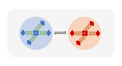
Figure 1: Schematic diagram of the model for numerical demonstrations. The $|a\rangle$ and $|b\rangle$ are the two electronic states of the molecule. Included are also the vibrational normal modes. They all interact with the solvent composed of harmonic oscillators. When the state transits between $|a\rangle$ and $|b\rangle$, the normal modes and the solvent oscillators are all displaced and reorganized.

III.2 Model of ET system

We set $\hbar=1$ in the following part of this section. Consider an ET system with the total Hamiltonian being

$$H_{\mbox{\tiny T}}=H_{a}|a\rangle\langle a|+(H_{b}+E^{\circ})|b\rangle\langle b|+V(|a\rangle\langle b|+|b\rangle\langle a|).$$ (40)

Here, $E^{\circ}$ is the reaction endothermicity and $V$ is the transfer coupling strength. $H_{a}$ and $H_{b}$ are the nuclei–solvent Hamiltonians for the ET system in the donor and acceptor states, respectively. They are assumed of the Caldeira–Leggett’s model,[1, 2] i.e.

$$H_{a} =\sum_{n=1}^{N_{\mbox{\tiny vib}}}\frac{\Omega_{n}}{2}(\hat{p}_{n}^{2}+\hat{q}_{n}^{2})+\sum_{k=1}^{N_{\mbox{\tiny sol}}}\frac{\omega_{k}}{2}\Bigg{\{}\tilde{p}^{2}_{k}+\bigg{[}\tilde{x}_{k}-\bigg{(}\sum_{n=1}^{N_{\mbox{\tiny vib}}}\frac{c_{nk}}{\omega_{k}}\hat{q}_{n}\bigg{)}\bigg{]}^{2}\Bigg{\}},$$ (41)

and $H_{b}$ is similar to $H_{a}$ but with linearly displaced $\{q^{\prime}_{n}=q_{n}-D_{n}\}$ and $\{x^{\prime}_{k}=x_{k}-d_{k}\}$. The first term in Eq. (41) is the Hamiltonian of the involved intramolecular vibrational normal modes, denoted as $H_{\mbox{\tiny vib}}$ afterwards. The solvent Hamiltonian is

$$h_{\mbox{\tiny sol}}=\frac{1}{2}\sum_{k=1}^{N_{\mbox{\tiny sol}}}\omega_{k}(\tilde{p}^{2}_{k}+\tilde{x}^{2}_{k}).$$ (42)

$N_{\mbox{\tiny vib}}$ and $N_{\mbox{\tiny sol}}$ are the numbers of the degrees of freedom of the intramolecular normal modes and the solvent, respectively. See the schematic diagram of this model in Fig. 1.

Before going on, let us introduce the solvent force operators

$$\hat{X}_{n}=\sum_{k}c_{nk}\tilde{x}_{k}\quad{\rm and}\quad\hat{Y}=\sum_{k}\omega_{k}d_{k}\tilde{x}_{k}.$$ (43)

Their participation in the total Hamiltonian [Eq. (40)] will be seen soon later. Denote the involving solvent response functions as

$$\varphi^{xx}_{mn}(t) \equiv i\langle[\hat{X}^{\mbox{\tiny sol}}_{m}(t),\hat{X}_{n}]\rangle_{\mbox{\tiny sol}}=\sum_{k}c_{mk}c_{nk}\sin(\omega_{k}t)$$

$$=i\langle[\hat{X}^{\mbox{\tiny sol}}_{n}(t),\hat{X}_{m}]\rangle_{\mbox{\tiny sol}}=\varphi^{xx}_{nm}(t),$$ (44a)

$$\varphi^{xy}_{n}(t) \equiv i\langle[\hat{X}^{\mbox{\tiny sol}}_{n}(t),\hat{Y}]\rangle_{\mbox{\tiny sol}}=\sum_{k}\omega_{k}d_{k}c_{nk}\sin(\omega_{k}t)$$

$$=i\langle[\hat{Y}^{\mbox{\tiny sol}}(t),\hat{X}_{n}]\rangle_{\mbox{\tiny sol}},$$ (44b)

$$\varphi^{yy}(t) \equiv i\langle[\hat{Y}^{\mbox{\tiny sol}}(t),\hat{Y}]\rangle_{\mbox{\tiny sol}}=\sum_{k}\omega^{2}_{k}d^{2}_{k}\sin(\omega_{k}t),$$ (44c)

and for any function $f(t)$ the frequency resolution, $\tilde{f}(\omega)\equiv\int^{\infty}_{0}\!\!{\rm d}t\,e^{i\omega t}f(t)$. Here, $\hat{O}^{\mbox{\tiny sol}}(t)=e^{ih_{\mbox{\tiny sol}}t}\hat{O}e^{-ih_{\mbox{\tiny sol}}t}$ and $\langle\cdots\rangle_{\mbox{\tiny sol}}={\rm tr}_{\mbox{\tiny sol}}(\cdots e^{-\beta h_{\mbox{\tiny sol}}})/{\rm tr}_{\mbox{\tiny sol}}e^{-\beta h_{\mbox{\tiny sol}}}$.

Note that $|a\rangle\langle a|+|b\rangle\langle b|=1$ and the Huang–Rhys factor $S_{n}=D_{n}^{2}/2$. Denote also ${\hat{\sigma}_{b}}\equiv|b\rangle\langle b|$ and $\hat{V}_{\mbox{\tiny ET}}\equiv V(|a\rangle\langle b|+|b\rangle\langle a|)$. The total Hamiltonian of Eq. (40) can be recast in terms of Eq. (36) with $h_{\mbox{\tiny B}}=h_{\mbox{\tiny sol}}$,

$$H_{\mbox{\tiny S}0}=H_{\mbox{\tiny vib}}+\hat{V}_{\mbox{\tiny ET}}+\Big{[}E^{\circ}+\sum_{n=1}^{N_{\mbox{\tiny vib}}}{\Omega_{n}}(S_{n}-D_{n}\hat{q}_{n})\Big{]}{\hat{\sigma}_{b}},$$ (45)

the multi-dissipative-mode system-bath interaction term,

$$\sum_{u}\hat{Q}_{u}\hat{F}_{u}={\hat{\sigma}_{b}}\bigg{(}\sum_{n=1}^{N_{\mbox{\tiny vib}}}D_{n}\hat{X}_{n}-\hat{Y}\bigg{)}-\sum_{n=1}^{N_{\mbox{\tiny vib}}}\hat{q}_{n}\hat{X}_{n}\,,$$ (46)

and the multi-mode reorganization term,

$$\sum_{uv}E^{\mbox{\tiny re}}_{uv}\hat{Q}_{u}\hat{Q}_{v}=E^{\mbox{\tiny re}}_{bb}{\hat{\sigma}_{b}}+\sum_{n}E^{\mbox{\tiny re}}_{nb}\hat{q}_{n}{\hat{\sigma}_{b}}+\sum_{mn}E^{\mbox{\tiny re}}_{mn}\hat{q}_{m}\hat{q}_{n}\,,$$ (47)

where

$$\begin{split}E^{\mbox{\tiny re}}_{bb}&=\frac{1}{2}\Big{[}\sum_{mn}\tilde{\varphi}^{xx}_{mn}(0)D_{m}D_{n}-2\sum_{n}\tilde{\varphi}^{xy}_{n}(0)D_{n}+\tilde{\varphi}^{yy}(0)\Big{]},\\ E^{\mbox{\tiny re}}_{nb}&=\tilde{\varphi}^{xy}_{n}(0)-\sum_{m}\tilde{\varphi}^{xx}_{mn}(0)D_{m}\,,\qquad E^{\mbox{\tiny re}}_{mn}=\frac{1}{2}\tilde{\varphi}^{xx}_{mn}(0).\end{split}$$ (48)

Thus in the calculation of $A_{\mbox{\tiny hyb}}$ via Eq. (39) for the process of the ET molecule embedded into the solvent, the involved intermediate quantities in the integrands of Eq. (39) are $\{\langle\hat{X}_{n}{\hat{\sigma}_{b}}\rangle_{1}\}$, $\langle\hat{Y}{\hat{\sigma}_{b}}\rangle_{1}$, $\{\langle\hat{X}_{n}\hat{q}_{n}\rangle_{1}\}$, $\langle{\hat{\sigma}_{b}}\rangle_{2}$, $\{\langle\hat{q}_{n}{\hat{\sigma}_{b}}\rangle_{2}\}$, $\{\langle\hat{q}_{m}\hat{q}_{n}\rangle_{2}\}$. Here $\langle\cdots\rangle_{1}$ and $\langle\cdots\rangle_{2}$ are similar to Eq. (38a) and Eq. (38b), respectively. To obtain them, the DEOM approach[37, 38] for the above model [Eqs. (45)–(47)] will be very time-consuming. This can be overcome via the SBET developed in Sec. II as below.

III.3 Model to two-state system

Equation (40) can also be recast as

$$H_{\mbox{\tiny T}}=\Big{(}E^{\circ}+E^{\mbox{\tiny re}}_{bb}+\sum_{n}\Omega_{n}S_{n}\Big{)}{\hat{\sigma}_{b}}+\hat{V}_{\mbox{\tiny ET}}+{\hat{\sigma}_{b}}\hat{F}+H_{a}\,.$$ (49)

The induced overall vibration-plus-solvent force to the two–electronic–state system is

$$\hat{F}=\sum_{n}D_{n}\hat{X}_{n}-\hat{Y}+\sum_{n}\big{(}E^{\mbox{\tiny re}}_{nb}-\Omega_{n}D_{n}\big{)}\hat{q}_{n}\,.$$ (50)

The overall force-force response function is

$$\Phi(t)\equiv i\langle[\hat{F}^{(a)}(t),\hat{F}]\rangle_{a}\equiv i\langle[e^{iH_{a}t}\hat{F}e^{-iH_{a}t},\hat{F}]\rangle_{a}\,,$$ (51)

where $\langle\cdots\rangle_{a}\equiv{\rm Tr}_{a}(\cdots e^{-\beta H_{a}})/{\rm Tr}_{a}e^{-\beta H_{a}}$. Equations (49)–(50) constitute the multi-vibrational-mode generalization of the single-mode exciton system in Ref. 29. The overall response function can be obtained following the similar derivation there,[29] via its frequency resolution, $\widetilde{\Phi}(\omega)$. Assume the solvent effects on different vibrational normal modes are un-correlated, i.e. $\varphi^{xx}_{mn}(t)=\delta_{mn}\varphi^{xx}_{nn}(t)$, leading to also $E^{\mbox{\tiny re}}_{nb}=\tilde{\varphi}^{xy}_{n}(0)-\tilde{\varphi}^{xx}_{nn}(0)D_{n}$. Denote $\bar{D}_{n}\equiv E^{\mbox{\tiny re}}_{nb}-\Omega_{n}D_{n}$. We can obtain[29, 35]

$$\widetilde{\Phi}(\omega) =\sum_{n}[D_{n}^{2}\tilde{\varphi}^{xx}_{nn}(\omega)-2D_{n}\tilde{\varphi}^{xy}_{n}(\omega)]+\tilde{\varphi}^{yy}(\omega)$$

$$\quad+\sum_{n}[\bar{D}_{n}+D_{n}\tilde{\varphi}^{xx}_{nn}(\omega)-\tilde{\varphi}^{xy}_{n}(\omega)]^{2}\tilde{\phi}^{qq}_{nn}(\omega),$$ (52)

where[29, 1]

$$\tilde{\phi}^{qq}_{nn}(\omega)=\frac{\Omega_{n}}{\Omega_{n}^{2}-\omega^{2}-\Omega_{n}[\tilde{\varphi}^{xx}_{nn}(\omega)-\tilde{\varphi}^{xx}_{nn}(0)]}\,.$$ (53)

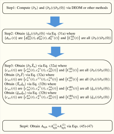
Figure 2: Flowchart for the calculation of the hybridization free energy. Step 1 only involves the calculation on a two-level system. In Steps 2 and 3, we first obtain $\phi_{nn}^{qx}(t)$, $\phi_{n}^{qy}(t)$, $\phi_{nn}^{xx}(t)$, $\phi_{n}^{xy}(t)$, and $\phi^{yy}(t)$ via SBET in Ref. 35. The first two use the Eq. (17) and the last three use the Eq. (18) of Ref. 35. The corresponding $c_{nn}^{qx}(t)$, $c_{n}^{qy}(t)$, $c_{nn}^{xx}(t)$, $c_{n}^{xy}(t)$, and $c^{yy}(t)$ are obtained via the FDT, Eq. (8).

Turn to the solvation free energy $A_{\mbox{\tiny hyb}}$ evaluation. As just mentioned, the key quantities to be calculated are $\{\langle\hat{X}_{n}{\hat{\sigma}_{b}}\rangle_{1}\}$, $\langle\hat{Y}{\hat{\sigma}_{b}}\rangle_{1}$, $\{\langle\hat{X}_{n}\hat{q}_{n}\rangle_{1}\}$, $\langle{\hat{\sigma}_{b}}\rangle_{2}$, $\{\langle\hat{q}_{n}{\hat{\sigma}_{b}}\rangle_{2}\}$, $\{\langle\hat{q}_{m}\hat{q}_{n}\rangle_{2}\}$. Given conditions are the solvent response functions [Eq. (44)] in terms of their frequency-domain resolutions, from which $\{\tilde{\phi}^{qq}_{nn}(\omega)\}$ and $\widetilde{\Phi}(\omega)$ are also determined. For each selected $\lambda$, the flowchart is shown in Fig. 2. The procedure repeats for $\lambda$ varying from 0 to 1 until the integrals in Eq. (39) are converged.

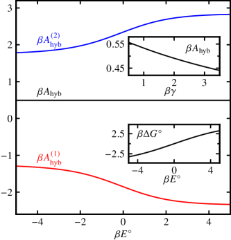
Figure 3: The hybridization free energy $A_{\mbox{\tiny hyb}}$ (in black), together with $A_{\mbox{\tiny hyb}}^{(1)}$ (in red) and $A_{\mbox{\tiny hyb}}^{(2)}$ (in blue), with respective to $E^{\circ}$. The temperature is $300$K. The main panel adopts $\beta\gamma=2$. See other parameters in the main text. The hybridization free energy (black line) changes very little with $E^{\circ}$, but more explicitly with $\gamma$ (upper inset). Depicted in the lower inset is $\beta\Delta G^{\circ}=-\ln K$ with $K$ being the equilibrium constant.

Figure 3 exhibits the obtained hybridization free energy $A_{\mbox{\tiny hyb}}$ with different values of the reaction endothermicity $E^{\circ}$. We choose $N_{\mbox{\tiny vib}}=2$. The temperature is $300$K. In the demonstration, we adopt

$$\begin{split}\tilde{\varphi}^{xx}_{nn}(\omega)=\frac{2\eta_{n}^{xx}\gamma}{\gamma-i\omega},\\ \tilde{\varphi}^{xy}_{n}(\omega)=\frac{2\eta_{n}^{xy}\gamma}{\gamma-i\omega},\\ \tilde{\varphi}^{yy}(\omega)=\frac{2\eta^{yy}\gamma}{\gamma-i\omega}.\end{split}$$ (54)

Parameters for the main panel of Fig. 3 are selected as $\beta V=1$, $\beta\Omega_{1}=4$, $\beta\Omega_{2}=1$, $D_{1}=D_{2}=0.5$, and $\beta\gamma=\beta\eta^{xx}_{11}=\beta\eta^{xx}_{22}=2$. We choose $\eta_{n}^{xy}=D_{n}\eta_{nn}^{xx}$ and $\eta^{yy}=\sum_{n}D_{n}^{2}\eta_{nn}^{xx}$ which constitutes the Brownian vibration condition.[29] In Fig. 3, it is observed that the total $A_{\mbox{\tiny hyb}}$ changes little with $E^{\circ}$, but changes more explicitly with the solvent friction $\gamma$ (upper inset). Depicted in the lower inset is $\beta\Delta G^{\circ}=-\ln K$ with $K$ being the equilibrium constant obtained from the computed equilibrium populations. The contribution of $A_{\mbox{\tiny hyb}}^{(1)}$ due to the solvent–solute interaction is negative, while that of $A_{\mbox{\tiny hyb}}^{(2)}$ due to the solvent reorganization is positive. They altogether amount to a positive $A_{\mbox{\tiny hyb}}$ which implies that external work is necessary for the reversible solute–solvent mixing. The absolute values of $A^{(1)}_{\mbox{\tiny hyb}}$ and $A^{(2)}_{\mbox{\tiny hyb}}$ share a similar behaviour with $\Delta G^{\circ}$, indicating their relevance with the extent of reaction. Note in our model for the molecule at the electronic state $a$ or $b$, its interaction with the solvent is actually of the same effect. Thus $A_{\rm hyb}$ is nearly unchanged in the reaction system $a\rightleftharpoons b$ with different system endothermicity $E^{\circ}$.

IV Summary

To summarize, this work generalizes the system–bath entanglement theorem (SBET), previously established for response functions,[35] to correlation functions. The derivation involves the use of generalized Langevin dynamics for the hybridizing bath modes and the Bogoliubov transformation. The latter maps the finite–temperature canonical reservoir to an effective zero–temperature vacuum. As a result, the generalized SBET connects the system–bath entanglement correlations to the local system and bare bath ones. It facilitates the evaluation of system–bath entangled correlations and bath mode correlations in the full composite space.

The demonstrations are carried out on computing the solvation free energy of an electron transfer system with specific intramolecular vibrational modes, exhibiting the practical utility of the generalized SBET. Particularly, based on the SBET, we develop a multi-scale approach to investigate the solvation effects, by only computing the electronic subsystem. In this approach, we separate different dynamical scales into electronic, vibrational and solvent parts. The SBET connects different scales rigorously and largely reduces computing cost, without any loss of important information such as environmental memory and cross–scale correlations. This provides an approach to investigate the large scale effects by only computing the small center system.

Appendix A Bogoliubov transformation

In order to perform the Bogoliubov transformation,[36] we shall first double the bath degrees of freedom by adopting an auxiliary bath as

$$h_{\mbox{\tiny B}}^{\prime}=-\sum_{j}\hbar\omega_{j}\hat{a}_{j}^{\prime\dagger}\hat{a}^{\prime}_{j}.$$ (55)

We will see later that the effective bath Hamiltonian [cf. Eq. (2)]

$$\tilde{h}_{\mbox{\tiny B}}\equiv h_{\mbox{\tiny B}}+h_{\mbox{\tiny B}}^{\prime}$$ (56)

retain the same form as $h_{\mbox{\tiny B}}+h_{\mbox{\tiny B}}^{\prime}=\sum_{j}\hbar\omega_{j}(\hat{a}_{j}^{\dagger}\hat{a}_{j}-\hat{a}_{j}^{\prime\dagger}\hat{a}^{\prime}_{j})$ after the transformation [Eq. (60)]. Define the Bogoliubov transformation,

$$\hat{d}_{j} \equiv\sqrt{\bar{n}_{j}+1}\hat{a}^{\prime}_{j}-\sqrt{\bar{n}_{j}}\hat{a}^{\dagger}_{j},$$ (57a)

$$\hat{d}^{\prime}_{j} \equiv\sqrt{\bar{n}_{j}+1}\hat{a}_{j}-\sqrt{\bar{n}_{j}}\hat{a}^{\prime\dagger}_{j}.$$ (57b)

The inverse transformation reads

$$\hat{a}_{j} =\sqrt{\bar{n}_{j}+1}\hat{d}^{\prime}_{j}+\sqrt{\bar{n}_{j}}\hat{d}_{j}^{\dagger},$$ (58a)

$$\hat{a}^{\prime}_{j} =\sqrt{\bar{n}_{j}+1}\hat{d}_{j}+\sqrt{\bar{n}_{j}}\hat{d}_{j}^{\prime\dagger}.$$ (58b)

It is easy to verify the transformation conserve the canonical commutators,

$$\begin{split}&[\hat{d}^{\prime}_{j},\hat{d}^{\prime}_{k}]=[\hat{d}^{\prime}_{j},\hat{d}_{k}]=[\hat{d}^{\prime}_{j},\hat{d}^{\dagger}_{k}]=[\hat{d}_{j},\hat{d}_{k}]=0,\\ &[\hat{d}^{\prime}_{j},\hat{d}_{k}^{\prime\dagger}]=[\hat{d}_{j},\hat{d}_{k}^{\dagger}]=\delta_{jk}.\end{split}$$ (59)

After the Bogoliubov transformation, we have that

$$h_{\mbox{\tiny B}}+h_{\mbox{\tiny B}}^{\prime}=\sum_{j}\hbar\omega_{j}(\hat{d}^{\prime\dagger}_{j}\hat{d}^{\prime}_{j}-\hat{d}^{\dagger}_{j}\hat{d}_{j}).$$ (60)

Now consider the state

$$|\xi\rangle\equiv\prod_{j}|\xi_{j}\rangle\ \ {\rm with}\ \ |\xi_{j}\rangle=\frac{1}{\sqrt{Z_{j}}}\sum_{n_{j}=0}^{\infty}e^{-n_{j}\beta\hbar\omega_{j}/2}|n_{j}\rangle|n_{j}\rangle^{\prime}.$$ (61)

Here, we introduce the phonon’s number states $|n_{j}\rangle\equiv\frac{1}{\sqrt{n_{j}!}}(\hat{a}^{\dagger}_{j})^{n_{j}}|{\bf 0}\rangle_{\mbox{\tiny B}}$ and $|n_{j}\rangle^{\prime}\equiv\frac{1}{\sqrt{n_{j}!}}(\hat{a}^{\prime\dagger}_{j})^{n_{j}}|{\bf 0}\rangle_{\mbox{\tiny B}}^{\prime}$, for the original bath $h_{\mbox{\tiny B}}$ and the auxiliary bath $h_{\mbox{\tiny B}}^{\prime}$, respectively. $Z_{j}\equiv(1-e^{-\beta\hbar\omega_{j}})^{-1}$ is the partition function for the harmonic mode of frequency $\omega_{j}$. It is easy to see that for the $\rho_{\mbox{\tiny B}}^{\rm eq}=e^{-\beta h_{\mbox{\tiny B}}}/{\rm tr}_{\mbox{\tiny B}}e^{-\beta h_{\mbox{\tiny B}}}$ as in Eq. (4), there is

$$\rho_{\mbox{\tiny B}}^{\rm eq}={\rm tr}_{\mbox{\tiny B}}^{\prime}\left(|\xi\rangle\langle\xi|\right),$$ (62)

where ${\rm tr}^{\prime}_{\mbox{\tiny B}}$ is the partial trace over the auxiliary bath space. Furthermore we have

$$\sqrt{Z_{j}}\hat{d}^{\prime}_{j}|\xi_{j}\rangle= \sum_{n_{j}=0}^{\infty}\!\!e^{-n_{j}\beta\hbar\omega_{j}/2}\big{(}\sqrt{\bar{n}_{j}+1}\hat{a}_{j}-\sqrt{\bar{n}_{j}}\hat{a}_{j}^{\prime\dagger}\big{)}|n_{j}\rangle|n_{j}\rangle^{\prime}$$

$$= \sum_{n_{j}=1}^{\infty}e^{-n_{j}\beta\hbar\omega_{j}/2}\sqrt{\bar{n}_{j}+1}\sqrt{n_{j}}|n_{j}-1\rangle|n_{j}\rangle^{\prime}$$

$$-\sum_{n_{j}=0}^{\infty}e^{-n_{j}\beta\hbar\omega_{j}/2}\sqrt{\bar{n}_{j}}\sqrt{n_{j}+1}|n_{j}\rangle|n_{j}+1\rangle^{\prime},$$

$$= \sum_{n_{j}=0}^{\infty}e^{-(n_{j}+1)\beta\hbar\omega_{j}/2}\sqrt{1+\bar{n}_{j}}\sqrt{n_{j}+1}|n_{j}\rangle|n_{j}+1\rangle^{\prime}$$

$$-\sum_{n_{j}=0}^{\infty}e^{-n_{j}\beta\hbar\omega_{j}/2}\sqrt{\bar{n}_{j}}\sqrt{n_{j}+1}|n_{j}\rangle|n_{j}+1\rangle^{\prime},$$

$$= \sum_{n_{j}=0}^{\infty}\!\!e^{-n_{j}\beta\hbar\omega_{j}/2}\big{(}e^{-\beta\hbar\omega_{j}/2}\sqrt{\bar{n}_{j}+1}-\sqrt{\bar{n}_{j}}\big{)}$$

$$\times\sqrt{n_{j}+1}|n_{j}\rangle|n_{j}+1\rangle^{\prime}=0.$$

In the last step, we have used the relation $e^{-\beta\hbar\omega_{j}}={\bar{n}_{j}}/(\bar{n}_{j}+1)$. Similarly, we can obtain also $\hat{d}_{j}|\xi_{j}\rangle=0$. It is thus proved that the state, $|\xi\rangle$, is actually the vacuum state of the effective bath $\tilde{h}_{\mbox{\tiny B}}$.

Appendix B Detailed–balance relation

In the canonical thermodynamic equilibrium condition, there is

$$\langle\hat{A}(t) \hat{B}(0)\rangle_{\rm eq}={\rm Tr}\big{(}e^{iH_{\mbox{\tiny T}}t/\hbar}\hat{A}e^{-iH_{\mbox{\tiny T}}t/\hbar}\hat{B}\rho_{\rm eq}\big{)},$$ (63)

with $\rho_{\rm eq}$ defined in Eq. (35). The detailed–balance relation reads

$$\langle\hat{A}(t)\hat{B}(0)\rangle^{\ast}_{\rm eq}=\langle\hat{A}(t-i\beta\hbar)\hat{B}(0)\rangle_{\rm eq}\,.$$ (64)

To prove Eq. (31) satisfy Eq. (64) in the condition of $\rho_{\rm st}=\rho_{\rm eq}$, we recast the main terms involved in Eq. (31) in a unified form as [cf. Eqs. (10), (23) and (25) together with some variables’ changes of the involved integrals]

$${\cal C}(t) \equiv{\rm Im}\bigg{[}\int_{0}^{\infty}\!\!{\mathrm{d}}\tau\,c_{uu^{\prime}}(t+\tau)C_{OO^{\prime}}(\tau)\bigg{]}$$

$$\quad+\int_{0}^{t}\!{\mathrm{d}}\tau\,{\rm Im}[c_{uu^{\prime}}(t-\tau)]C_{O^{\prime}O}(\tau).$$ (65)

Here, $\hat{O}$ and $\hat{O}^{\prime}$ are arbitrary Hermitian operators of the system or bath. We need to prove ${\cal C}^{\ast}(t)={\cal C}(t-i\beta\hbar)$. To do that we further expand Eq. (B) into four terms as

$${\cal C}(t) =\frac{i}{2}\int_{0}^{\infty}\!\!{\mathrm{d}}\tau\,c^{\ast}_{uu^{\prime}}(t+\tau)C^{\ast}_{OO^{\prime}}(\tau)$$

$$\quad-\frac{i}{2}\int_{0}^{\infty}\!\!{\mathrm{d}}\tau\,c_{uu^{\prime}}(t+\tau)C_{OO^{\prime}}(\tau)$$

$$\quad+\frac{i}{2}\int_{0}^{t}\!{\mathrm{d}}\tau\,c^{\ast}_{uu^{\prime}}(t-\tau)C_{O^{\prime}O}(\tau)$$

$$\quad-\frac{i}{2}\int_{0}^{t}\!{\mathrm{d}}\tau\,c_{uu^{\prime}}(t-\tau)C_{O^{\prime}O}(\tau)$$

$$\equiv\frac{\hbar}{2}\big{[}{\cal C}_{1}(t)+{\cal C}_{2}(t)+{\cal C}_{3}(t)+{\cal C}_{4}(t)\big{]}.$$ (66)

Let us denote the eigenstate and eigenenergy of the bath Hamiltonian $h_{\mbox{\tiny B}}$ as $|m\rangle$ and $\varepsilon_{m}$, i.e. $h_{\mbox{\tiny B}}|m\rangle=\varepsilon_{m}|m\rangle$. Denote the eigenstate and eigenenergy of the total Hamiltonian $H_{\mbox{\tiny T}}$ as $|\alpha\rangle$ and $E_{\alpha}$, i.e. $H_{\mbox{\tiny T}}|\alpha\rangle=E_{\alpha}|\alpha\rangle$. We can then recast $c_{uu^{\prime}}(t)$ [Eq. (7)] and $C_{OO^{\prime}}(t)$ [Eq. (63) or Eq. (II.1) with $\rho_{\rm st}=\rho_{\rm eq}$] as the following expressions, respectively,

$$c_{uu^{\prime}}(t) =\frac{1}{Z_{\mbox{\tiny B}}}\sum_{m,m^{\prime}}e^{i(\varepsilon_{m}-\varepsilon_{m^{\prime}})t/\hbar}e^{-\beta\varepsilon_{m}}F_{u;mm^{\prime}}F_{u^{\prime};m^{\prime}m}\,,$$ (67)

and

$$C_{OO^{\prime}}(t)=\frac{1}{Z_{\mbox{\tiny T}}}\sum_{\alpha,\alpha^{\prime}}e^{i(E_{\alpha}-E_{\alpha^{\prime}})t/\hbar}e^{-\beta E_{\alpha}}O_{\alpha\alpha^{\prime}}O^{\prime}_{\alpha^{\prime}\alpha}\,.$$ (68)

Substituting into Eq. (B), we obtain

$${\cal C}_{1}(t) =\frac{1}{Z_{\mbox{\tiny B}}Z_{\mbox{\tiny T}}}\sum_{m,m^{\prime}}\sum_{\alpha,\alpha^{\prime}}e^{i(\varepsilon_{m}-\varepsilon_{m^{\prime}})t/\hbar}e^{-\beta(\varepsilon_{m^{\prime}}+E_{\alpha^{\prime}})}$$

$$\quad\times F_{u;mm^{\prime}}F_{u^{\prime};m^{\prime}m}O_{\alpha\alpha^{\prime}}O^{\prime}_{\alpha^{\prime}\alpha}$$

$$\quad\times\bigg{[}-\frac{1}{(\varepsilon_{m}-\varepsilon_{m^{\prime}})+(E_{\alpha}-E_{\alpha^{\prime}})}$$

$$\qquad\ \ \,+i\pi\delta(\varepsilon_{m}-\varepsilon_{m^{\prime}}+E_{\alpha}-E_{\alpha^{\prime}})\bigg{]},$$

$${\cal C}_{2}(t) =\frac{1}{Z_{\mbox{\tiny B}}Z_{\mbox{\tiny T}}}\sum_{m,m^{\prime}}\sum_{\alpha,\alpha^{\prime}}e^{i(\varepsilon_{m}-\varepsilon_{m^{\prime}})t/\hbar}e^{-\beta(\varepsilon_{m}+E_{\alpha})}$$

$$\quad\times F_{u;mm^{\prime}}F_{u^{\prime};m^{\prime}m}O_{\alpha\alpha^{\prime}}O^{\prime}_{\alpha^{\prime}\alpha}$$

$$\quad\times\bigg{[}\frac{1}{(\varepsilon_{m}-\varepsilon_{m^{\prime}})+(E_{\alpha}-E_{\alpha^{\prime}})}$$

$$\qquad\ \ \,-i\pi\delta(\varepsilon_{m}-\varepsilon_{m^{\prime}}+E_{\alpha}-E_{\alpha^{\prime}})\bigg{]},$$

$${\cal C}_{3}(t) =\frac{1}{Z_{\mbox{\tiny B}}Z_{\mbox{\tiny T}}}\sum_{m,m^{\prime}}\sum_{\alpha,\alpha^{\prime}}e^{-\beta(\varepsilon_{m^{\prime}}+E_{\alpha^{\prime}})}F_{u;mm^{\prime}}F_{u^{\prime};m^{\prime}m}O_{\alpha\alpha^{\prime}}O^{\prime}_{\alpha^{\prime}\alpha}$$

$$\quad\times\frac{e^{i(\varepsilon_{m}-\varepsilon_{m^{\prime}})t/\hbar}-e^{-i(E_{\alpha}-E_{\alpha^{\prime}})t/\hbar}}{(\varepsilon_{m}-\varepsilon_{m^{\prime}})+(E_{\alpha}-E_{\alpha^{\prime}})}\,,$$

$${\cal C}_{4}(t) =\frac{1}{Z_{\mbox{\tiny B}}Z_{\mbox{\tiny T}}}\sum_{m,m^{\prime}}\sum_{\alpha,\alpha^{\prime}}e^{-\beta(\varepsilon_{m}+E_{\alpha^{\prime}})}F_{u;mm^{\prime}}F_{u^{\prime};m^{\prime}m}O_{\alpha\alpha^{\prime}}O^{\prime}_{\alpha^{\prime}\alpha}$$

$$\quad\times\frac{e^{-i(E_{\alpha}-E_{\alpha^{\prime}})t/\hbar}-e^{i(\varepsilon_{m}-\varepsilon_{m^{\prime}})t/\hbar}}{(\varepsilon_{m}-\varepsilon_{m^{\prime}})+(E_{\alpha}-E_{\alpha^{\prime}})}\,.$$

Altogether, we have

$${\cal C}(t) =\frac{\hbar}{2Z_{\mbox{\tiny B}}Z_{\mbox{\tiny T}}}\sum_{m,m^{\prime}}\sum_{\alpha,\alpha^{\prime}}\frac{F_{u;mm^{\prime}}F_{u^{\prime};m^{\prime}m}O_{\alpha\alpha^{\prime}}O^{\prime}_{\alpha^{\prime}\alpha}}{(\varepsilon_{m}-\varepsilon_{m^{\prime}})+(E_{\alpha}-E_{\alpha^{\prime}})}$$

$$\quad\times\Big{\{}e^{-i(E_{\alpha}-E_{\alpha^{\prime}})t/\hbar}\big{[}{e^{-\beta(\varepsilon_{m}+E_{\alpha^{\prime}})}-e^{-\beta(\varepsilon_{m^{\prime}}+E_{\alpha^{\prime}})}}\big{]}$$

$$\qquad\ +e^{i(\varepsilon_{m}-\varepsilon_{m^{\prime}})t/\hbar}\big{[}e^{-\beta(\varepsilon_{m}+E_{\alpha})}-e^{-\beta(\varepsilon_{m}+E_{\alpha^{\prime}})}\big{]}\Big{\}}\,.$$ (69)

We can thus easily find ${\cal C}^{\ast}(t)={\cal C}(t-i\beta\hbar)$ by Eq. (B). It is then straightforward to finish the proof that the SBET [Eq. (31)], established in general for steady states, satisfies the detailed–balance relation at the condition of the thermal canonical equilibrium.

References

- [1] U. Weiss, Quantum Dissipative Systems, World Scientific, Singapore, 2021, 5th ed.
- [2] A. O. Caldeira and A. J. Leggett, “Path integral approach to quantum Brownian motion,” Physica A 121, 587 (1983).
- [3] H. Grabert, P. Schramm, and G. L. Ingold, “Quantum Brownian motion: The functional integral approach,” Phys. Rep. 168, 115 (1988).
- [4] G. Lindblad, “Brownian motion of a quantum harmonic oscillator,” Rep. Math. Phys. 10, 393 (1976).
- [5] R. K. Wangsness and F. Bloch, “The dynamical theory of nuclear induction,” Phys. Rev. 89, 728 (1953).
- [6] F. Bloch, “Generalized theory of relaxation,” Phys. Rev. 105, 1206 (1957).
- [7] A. G. Redfield, “The theory of relaxation processes,” Adv. Magn. Reson. 1, 1 (1965).
- [8] Y. J. Yan, F. Shuang, R. X. Xu, J. X. Cheng, X. Q. Li, C. Yang, and H. Y. Zhang, “Unified approach to the Bloch-Redfield theory and quantum Fokker-Planck equations,” J. Chem. Phys. 113, 2068 (2000).
- [9] L. Diósi and W. T. Strunz, “The non-Markovian stochastic Schrödinger equation for open systems,” Phys. Lett. A 235, 569 (1997).
- [10] J. T. Stockburger and C. H. Mak, “Stochastic Liouvillian algorithm to simulate dissipative quantum dynamics with arbitrary precision,” J. Chem. Phys. 110, 4983 (1999).
- [11] J. S. Shao, “Decoupling quantum dissipation interaction via stochastic fields,” J. Chem. Phys. 120, 5053 (2004).
- [12] C.-Y. Hsieh and J. S. Cao, “A unified stochastic formulation of dissipative quantum dynamics. I. Generalized hierarchical equations,” J. Chem. Phys. 148, 014103 (2018).
- [13] C.-Y. Hsieh and J. S. Cao, “A unified stochastic formulation of dissipative quantum dynamics. II. Beyond linear response of spin baths,” J. Chem. Phys. 148, 014104 (2018).
- [14] Y. C. Wang, Y. L. Ke, and Y. Zhao, “The hierarchical and perturbative forms of stochastic Schrödinger equations and their applications to carrier dynamics in organic materials,” WIREs Comput. Mol. Sci. 9, e1375 (2019).
- [15] Y. A. Yan, “Stochastic simulation of anharmonic dissipation. II. Harmonic bath potentials with quadratic couplings,” J. Chem. Phys. 150, 074106 (2019).
- [16] Z. H. Chen, Y. Wang, R. X. Xu, and Y. J. Yan, “Quantum dissipation with nonlinear environment couplings: Stochastic fields dressed dissipaton equation of motion approach,” J. Chem. Phys. 155, 174111 (2021).
- [17] H. B. Wang and M. Thoss, “Multilayer formulation of the multiconfiguration time-dependent Hartree theory,” J. Chem. Phys. 119, 1289 (2003).
- [18] R. P. Feynman and F. L. Vernon, Jr., “The theory of a general quantum system interacting with a linear dissipative system,” Ann. Phys. 24, 118 (1963).
- [19] N. Makri, “Improved Feynman propagators on a grid and non-adiabatic corrections within the path integral framework,” Chem. Phys. Lett. 193, 435 (1992).
- [20] N. Makri and D. E. Makarov, “Tensor propagator for iterative quantum time evolution of reduced density matrices. I. Theory,” J. Chem. Phys. 102, 4600 (1995).
- [21] N. Makri and D. E. Makarov, “Tensor propagator for iterative quantum time evolution of reduced density matrices. II. Numerical methodology,” J. Chem. Phys. 102, 4611 (1995).
- [22] Y. Tanimura, “Nonperturbative expansion method for a quantum system coupled to a harmonic-oscillator bath,” Phys. Rev. A 41, 6676 (1990).
- [23] Y. A. Yan, F. Yang, Y. Liu, and J. S. Shao, “Hierarchical approach based on stochastic decoupling to dissipative systems,” Chem. Phys. Lett. 395, 216 (2004).
- [24] R. X. Xu, P. Cui, X. Q. Li, Y. Mo, and Y. J. Yan, “Exact quantum master equation via the calculus on path integrals,” J. Chem. Phys. 122, 041103 (2005).
- [25] Y. Tanimura, “Numerically “exact” approach to open quantum dynamics: The hierarchical equations of motion (HEOM),” J. Chem. Phys 153, 020901 (2020).
- [26] U. Fano, “Effects of configuration interaction on intensities and phase shifts,” Phys. Rev. 124, 1866 (1961).
- [27] Y. Zhang, T.-T. Tang, C. Girit, Z. Hao, M. C. Martin, A. Zettl, M. F. Crommie, Y. R. Shen, and F. Wang, “Direct observation of a widely tunable bandgap in bilayer graphene,” Nature 459, 820 (2009).
- [28] A. E. Miroshnichenko, S. Flach, and Y. S. Kivshar, “Fano resonances in nanoscale structures,” Rev. Mod. Phys. 82, 2257 (2010).
- [29] Z. H. Chen, Y. Wang, R. X. Xu, and Y. J. Yan, “Correlated vibration-solvent effects on the non-Condon exciton spectroscopy,” J. Chem. Phys. 154, 244105 (2021).
- [30] Y. Wang, Z. H. Chen, R. X. Xu, X. Zheng, and Y. J. Yan, “A statistical quasi–particles thermofield theory with Gaussian environments: System–bath entanglement theorem for nonequilibrium correlation functions,” J. Chem. Phys. 157, 044012 (2022).
- [31] Y. J. Yan, “Theory of open quantum systems with bath of electrons and phonons and spins: Many-dissipaton density matrixes approach,” J. Chem. Phys. 140, 054105 (2014).
- [32] H. D. Zhang, R. X. Xu, X. Zheng, and Y. J. Yan, “Nonperturbative spin-boson and spin-spin dynamics and nonlinear Fano interferences: A unified dissipaton theory based study,” J. Chem. Phys. 142, 024112 (2015).
- [33] R. X. Xu, H. D. Zhang, X. Zheng, and Y. J. Yan, “Dissipaton equation of motion for system-and-bath interference dynamics,” Sci. China Chem. 58, 1816 (2015), Special Issue: Lemin Li Festschrift.
- [34] Y. Wang and Y. J. Yan, “Quantum mechanics of open systems: Dissipaton theories,” J. Chem. Phys. 157, 170901 (2022).
- [35] P. L. Du, Y. Wang, R. X. Xu, H. D. Zhang, and Y. J. Yan, “System-bath entanglement theorem with Gaussian environments,” J. Chem. Phys. 152, 034102 (2020).
- [36] H. Umezawa, Advanced Field Theory: Micro, Macro, and Thermal Physics, Springer, New York, 1995.
- [37] H. Gong, Y. Wang, H. D. Zhang, Q. Qiao, R. X. Xu, X. Zheng, and Y. J. Yan, “Equilibrium and transient thermodynamics: A unified dissipaton–space approach,” J. Chem. Phys. 153, 154111 (2020).
- [38] H. Gong, Y. Wang, H. D. Zhang, R. X. Xu, X. Zheng, and Y. J. Yan, “Thermodynamic free–energy spectrum theory for open quantum systems,” J. Chem. Phys. 153, 214115 (2020).
- [39] J. G. Kirkwood, “Statistical mechanics of fluid mixtures,” J. Chem. Phys. 3, 300 (1935).
- [40] R. van Zon, L. Hernández de la Peña, G. H. Peslherbe, and J. Schofield, “Quantum free-energy differences from nonequilibrium path integrals. I. Methods and numerical application,” Phys. Rev. E 78, 041103 (2008).
- [41] R. van Zon, L. Hernández de la Peña, G. H. Peslherbe, and J. Schofield, “Quantum free-energy differences from nonequilibrium path integrals. II. Convergence properties for the harmonic oscillator,” Phys. Rev. E 78, 041104 (2008).