Structure-Aware Path Inference
for Neural Finite State Transducers

Abstract

Neural finite-state transducers (NFSTs) form an expressive family of neurosymbolic sequence transduction models. An NFST models each string pair as having been generated by a latent path in a finite-state transducer. As they are deep generative models, both training and inference of NFSTs require inference networks that approximate posterior distributions over such latent variables. In this paper, we focus on the resulting challenge of imputing the latent alignment path that explains a given pair of input and output strings (e.g., during training). We train three autoregressive approximate models for amortized inference of the path, which can then be used as proposal distributions for importance sampling. All three models perform lookahead. Our most sophisticated (and novel) model leverages the FST structure to consider the graph of future paths; unfortunately, we find that it loses out to the simpler approaches—except on an artificial task that we concocted to confuse the simpler approaches.

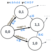
Figure 1: Marked finite-state transducer, all of whose paths generate input $\bm{x}$ and output $\bm{y}$. We show the transitions from the initial state, with their input:output symbols and marks. The same example appears in Fig. 3 without the marks shown.

1 Introduction

Recent advances in applied deep learning have typically applied end-to-end training to homogeneous architectures such as recurrent neural nets (RNNs) [rnn], convolutional neural networks [convnet], or Transformers [transformer]. For small-data settings, however, end-to-end training can benefit from inductive bias through domain-specific constraints and featurization [rastogi-etal-2016-weighting]. In the case of sequence-to-sequence problems—e.g., grapheme-to-phoneme [knight-graehl-1998-machine] or speech-to-text [mohri2008speech]—one technique is to use finite-state transducers (FSTs), which were widely used in NLP, speech recognition, and text processing before the deep learning revolution [mohri-1997, EFSML-1999, allauzen2007openfst, mohri2008speech]. An FST’s topology can be manually designed based on the task of interest. In this paper, we design and compare inference networks for use with “neuralized” FSTs.

Neuralized FSTs (NFSTs) [lin-etal-2019-neural] abandon the Markov property to become more expressive than standard arc-weighted FSTs [eisner-2002-parameter]. A path’s weight is computed by some arbitrary neural model from the ordered string of marks encountered along the path. The marks on each arc provide features of the transduction operation carried out by that arc (as illustrated in Fig. 1).

However, the expressiveness of NFSTs comes at the cost of training efficiency. Modeling joint or conditional probabilities on observed string pairs $(\bm{x},\bm{y})$ requires imputing the latent NFST path $\bm{z}$ that aligns each observed input string $\bm{x}$ with its output string $\bm{y}$, as we review in § 2. Summing over these paths is expensive because NFSTs give up the Markov property that enables dynamic programming on traditional weighted FSTs [mohri2002]. We must fall back on importance sampling. To this end, lin-etal-2019-neural built an autoregressive proposal distribution for these latent paths.

Their proposal distribution—basically the SWS method described in § 3.2 below—sampled a path through the NSFT from left to right. At each step, the choice of the next arc was influenced by the prefix path sampled so far and by the suffixes of $\bm{x}$ and $\bm{y}$ that have yet to be aligned. In this paper, we extend this idea (§ 3.3) to consider the graph of possible alignments of those suffixes (Fig. 3), as determined by the NFST topology. We evaluated the quality of the proposal distributions on three tasks:

• (tr) reverse transliteration of Urdu words from the Roman alphabet to the Urdu alphabet

• (scan) compositional navigation commands paired with the corresponding action sequences

• (cipher) synthetic dataset created by enciphering the input text with certain patterns

Task examples are shown in LABEL:table::dataset, and more descriptions are available in LABEL:app::dataset. We compared our novel proposal distribution (§ 3.3) to the approach of [lin-etal-2019-neural] (§ 3.2) and to an even simpler baseline (§ 3.1). Overall, it was difficult to get our novel method to work. In the tr and scan tasks, it is apparently possible to choose the next arc well enough by the existing method of looking ahead to the unaligned suffixes. Perhaps the existing method learns to compare their lengths or their unordered bags of symbols. We designed the cipher task to frustrate such heuristics, and there our novel method really was necessary, benefiting from its domain knowledge of possible alignments (the given FST). But for the tr and scan tasks, our novel proposal distribution did considerably worse—perhaps our architecture was unnecessarily complicated and harder to train. This raises questions about the necessity and wisdom of explicitly considering the graph of possible alignments for real-world tasks.

2 Preliminaries: Neuralized Finite-State Transducers

2.1 Marked FSTs

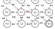
Figure 2: Directed graph constructed by composing an edit-distance MFST ${\cal T}$ with input $\bm{x}=abc$ and output $\bm{y}=cd$. The marks are suppressed here, but see Fig. 1.

A marked FST, or MSFT, is a directed graph in which some states are designated as initial and/or final, and each arc is labeled with an input substring, an output substring, and a mark substring. An generating path in the MFST is any path $\bm{z}$ from an initial state to a final state. It is said to generate the pair $(\bm{x},\bm{y})$ with mark string $\bm{\omega}$ if $\bm{x},\bm{y},\bm{\omega}$ respectively are the concatenations of the input, output, and mark substrings of $\bm{z}$’s arcs.

The mark string on a generating path of $\cal T$ provides domain-specific information about the path. It may record information about the states along the path, the symbols being generated (for example, their phonetic or orthographic properties), how the path aligns input and output symbols (that is, which symbols or properties are being edited), and the contexts of these aligned symbols (for example, whether they fall in the onset, nucleus, or coda of a linguistic syllable). We may compose the MFST ${\cal T}$ with strings $\bm{x},\bm{y}$ to obtain a restricted FST $\bm{x}\circ\mathcal{T}\circ\bm{y}$ whose generating paths correspond exactly to the paths in ${\cal T}$ that generate $(\bm{x},\bm{y})$, with the same marks. A standard simple example is shown in Fig. 2: input "abc" and output "cd" have been composed with a 1-state MFST whose arcs (which are self-loops) allow symbol insertions, deletions, and substitutions. The generating paths are the paths from $(0,0)$ to $(3,2)$. The red path in Fig. 2 transforms "abc" to "cd" by deleting the second symbol of "abc" and substituting for the others.

2.2 Neuralized FSTs

A neuralized finite-state transducer (NFST) is an MFST ${\cal T}$ paired with some parametric scoring function $\tilde{p}_{\theta}$ that maps any generating path’s mark string to a non-negative weight. Given an appropriate ${\cal T}$, this defines an unnormalized probability distribution $\tilde{p}_{\theta}$ over the paths. See LABEL:app::NFST_def for a formal definition.

In practice, we will estimate $\tilde{p}_{\theta}$ by estimating its parameters $\theta$. The unnormalized probability of a string pair is obtained by summing over the paths $\bm{z}$ that might have generated that string:

$$\tilde{p}_{\theta}({\bm{x}},{\bm{y}})\mathrel{\stackrel{{\scriptstyle\textnormal{\tiny def}}}{{=}}}\textstyle\sum_{{\bm{z}}\in\bm{x}\circ\mathcal{T}\circ\bm{y}}\tilde{p}_{\theta}(\bm{z})$$ (1)

Given the pair $(\bm{x},\bm{y})$, the posterior distribution over the latent generating path $\bm{z}\in\bm{x}\circ\mathcal{T}\circ\bm{y}$ is $p_{\theta}(\bm{z}\mid\bm{x},\bm{y})\mathrel{\stackrel{{\scriptstyle\textnormal{\tiny def}}}{{=}}}\tilde{p}_{\theta}({\bm{z}})/\tilde{p}_{\theta}({\bm{x}},{\bm{y}})$. We emphasize that $\tilde{p}_{\theta}(\bm{z})$ depends on $\bm{z}$ only through its mark string.

Computing the quantity $\log\tilde{p}_{\theta}({\bm{x}},{\bm{y}})$ is crucial for training $\theta$. However, equation 1’s marginalization over mark strings $\bm{z}$ is in general intractable. We resort to using a Monte Carlo variational lower bound, which imputes $\bm{z}\sim p_{\theta}(\cdot\mid\bm{x},\bm{y})$ by importance sampling using a neural proposal distribution $q_{\phi}(\bm{z}\mid\bm{x},\bm{y})\approx p_{\theta}(\bm{z}\mid\bm{x},\bm{y})$. In LABEL:app::NFST_train we describe a procedure for jointly training $p_{\theta}$ and $q_{\phi}$, making use of the importance weighting estimator [iwae] and making certain assumptions about $\cal T$ and $p_{\theta}$.

Our focus in this paper is to consider different parametric forms for the distribution $q_{\phi}$ over paths that generate $(\bm{x},\bm{y})$. To simplify our study, we assume that $\theta$ is given, and only train $\phi$ to minimize the divergence $\text{KL}(p_{\theta}\mathrel{\|}q_{\phi})=\underset{\bm{z}\sim p(\cdot\mid\bm{x},\bm{y})}{\mathbb{E}}[-\log q_{\phi}(\bm{z}\mid\bm{x},\bm{y})]$ by following its gradient (or rather, the biased estimate of its gradient that we obtain by normalized importance sampling, sample size 16).

3 Three Proposal Distributions

We explore three distribution families $q_{\phi}(\bm{z}\mid\bm{x},\bm{y})$, sketched in Fig. 3. Like $p_{\theta}$ itself, each $q_{\phi}$ family is insensitive to the specific topology and labeling of $\cal T$. Any MFST that was equivalent to $\cal T$ in the sense of generating the same set of $(\bm{x},\bm{y},\bm{\omega})$ triples—that is, the same regular 3-way relation—would give the same parametric proposal distribution $q_{\phi}$. Sampling from $q_{\phi}$ in each case is done by sampling a mark string $\bm{\omega}$ and using it to identify a path $\bm{z}$ in $\cal T$. To make this identification possible, we henceforth assume that distinct paths in $\cal T$ with the same $\bm{x},\bm{y}$ always have distinct mark strings. (A stronger assumption is already needed for the particular model $\tilde{p}_{\theta}$ that we spell out in LABEL:app::NFST_train.)

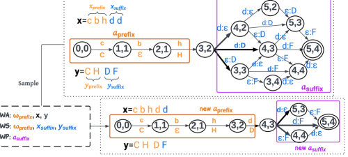
Figure 3: Choosing a generating path $\bm{a}$ in $\mathcal{T}_{\bm{x},\bm{y}}$ with mark string $\bm{\omega}$. (Note that $\bm{a}$ ranges over paths in $\mathcal{T}_{\bm{x},\bm{y}}$, whereas $\bm{z}$ ranges over paths in $\cal T$. Marks are not shown.) The top graph shows that after choosing the first 3 arcs $\bm{a}_{\text{prefix}}=a_{1}a_{2}a_{3}$, reaching state $(3,2)$, the sampler must choose a suffix path through the subgraph $\bm{a}_{\text{suffix}}$ of $\mathcal{T}_{\bm{x},\bm{y}}$ that is reachable from $(3,2)$. Its choices for $a_{4}$ are the three thick out-arcs from $(3,2)$; choosing the arc to $(4,3)$ yields the reduced graph of possible paths $\bm{a}$ at the bottom. To make its stochastic choice, the sampler (SWA, SWS, or SWP) conditions on certain properties of the top graph, shown in the dashed box at the left. Here $\bm{x}_{\text{prefix}},\bm{y}_{\text{prefix}},\bm{\omega}_{\text{prefix}}$ refer to the labels on $\bm{a}_{\text{prefix}}$, while $\bm{x}_{\text{suffix}},\bm{y}_{\text{suffix}}$ are the remaining portions of $\bm{x},\bm{y}$. SWP’s choice is determined by a global backward pass on $\mathcal{T}_{\bm{x},\bm{y}}$ in which the probabilities of the out-arcs depend only on $\bm{a}_{\text{suffix}}$.

Let $\mathcal{T}_{\bm{x},\bm{y}}$ be a version of $\bm{x}\circ\mathcal{T}\circ\bm{y}$ that has been determinized with respect to the mark tape and then minimized. Then $\mathcal{T}_{\bm{x},\bm{y}}$ is a canonical MFST that expresses the same relation as $\bm{x}\circ\mathcal{T}\circ\bm{y}$, while guaranteeing that (a) each arc’s mark substring has length 1, (b) the out-arcs from a state are labeled with different marks, and (c) every choice of out-arc can lead to a final state.

It follows that we can sample a mark string $\bm{\omega}$ by autoregressively sampling a generating path $\bm{a}$ in $\mathcal{T}_{\bm{x},\bm{y}}$, at each step requiring only a distribution over the out-arcs from the current state, or equivalently, over their distinct marks. We abuse notation and write $q_{\phi}$ for $q_{\phi}(\bm{a}\mid\mathcal{T}_{\bm{x},\bm{y}})$, $q_{\phi}(\bm{\omega}\mid\mathcal{T}_{\bm{x},\bm{y}})$, and $q_{\phi}(\bm{z}\mid\bm{x},\bm{y})$.

Since we use the standard minimization construction, $\mathcal{T}_{\bm{x},\bm{y}}$ is reduced, meaning that the input and output symbols on a path appear “as soon as possible” [reutenauer-1990]. This standardizes how the symbols are distributed along the path, ensuring that $\bm{x}_{\text{suffix}},\bm{y}_{\text{suffix}}$ are well-defined in the SWS sampler (§ 3.2).

3.1 Sampler with Attention (SWA)

The SWA sampler proposes the next mark $\omega_{t}$ in $\bm{\omega}$ by considering (1) the marks $\bm{\omega}_{<t}=\omega_{1}\cdots\omega_{t-1}$ already chosen and (2) an assessment of which marks might be chosen in future. For (1), we use a recurrent neural network to encode $\bm{\omega}_{<t}$ into a vector ${\bm{\mathbf{h}}}_{t-1}$. For (2), an attention mechanism is employed to mine information from the raw strings $(\bm{x},\bm{y})$. More formally, SWA samples from

$$q_{\phi}(\omega_{t}\mid\bm{\omega}_{<t},\mathcal{T}_{\bm{x},\bm{y}}) \propto\exp(W\,[1;{\bm{\mathbf{h}}}_{t-1};\text{Att}({\bm{\mathbf{h}}}_{t-1},\text{enc}(\bm{x},\bm{y}))])$$ (2)

meaning a softmax distribution over just the marks $\omega_{t}$ that $\mathcal{T}_{\bm{x},\bm{y}}$ allows to follow $\bm{\omega}_{<t}$. Equation 2 applies the learned matrix $W$ to the concatenation of the state ${\bm{\mathbf{h}}}_{t-1}$, which encodes $\bm{\omega}_{\text{prefix}}$, and $\text{Att}(\cdots)$ which uses ${\bm{\mathbf{h}}}_{t-1}$ to attend to $(\bm{x},\bm{y})$ (not necessarily just $\bm{x}_{\text{suffix}},\bm{y}_{\text{suffix}}$ in Fig. 3 We compute ${\bm{\mathbf{h}}}_{t-1}\in\mathbb{R}^{d}$ with a left-to-right GRU [gru], as in lin-eisner-2018-neural. We compute $\text{enc}(\bm{x},\bm{y})\in\mathbb{R}^{n\times d}$ by applying a separate bidirectional GRU to the concatenation $\bm{x}\#\bm{y}^{R}$, whose length we denote by $n$. We then use ${\bm{\mathbf{h}}}_{t-1}$ as a softmax-attention query over the $n$ encoded tokens of $\bm{x}\#\bm{y}^{R}$:

$$\text{Att}({\bm{\mathbf{h}}}_{t-1},\text{enc}(\bm{x},\bm{y}))=\sum_{i=1}^{n}a_{i}\,\text{enc}_{i}(\bm{x},\bm{y}),\text{\ \ \ \ where }a_{i}=\frac{\exp({\bm{\mathbf{h}}}_{t-1}\cdot\text{enc}_{i}(\bm{x},\bm{y}))}{\sum_{j=1}^{n}\exp({\bm{\mathbf{h}}}_{t-1}\cdot\text{enc}_{j}(\bm{x},\bm{y}))}$$ (3)

3.2 Sampler with State Tracking (SWS)

The SWS sampler is simpler than SWA (no attention), but it takes care to consider only the suffixes of $\bm{x}$ and $\bm{y}$ that remain to be aligned. The prefix path of $\mathcal{T}_{\bm{x},\bm{y}}$ marked with $\bm{\omega}_{<t}$ has generated aligned input and output strings $\bm{x}_{<t},\bm{y}_{<t}$ (which may not have length $t$). Let $\bm{x}_{\geq t}$ and $\bm{y}_{\geq t}$ denote the unaligned suffixes of $\bm{x},\bm{y}$, and encode them into vectors by $\text{enc}_{\text{x}}$ and $\text{enc}_{\text{y}}$, which are separate right-to-left GRUs. SWS samples from

$$q_{\phi}(\omega_{t}\mid\bm{\omega}_{<t},\mathcal{T}_{\bm{x},\bm{y}}) \propto\exp(W\,[1;{\bm{\mathbf{h}}}_{t-1};\text{enc}_{\text{x}}(\bm{x}_{\geq t});\text{enc}_{\text{y}}(\bm{y}_{\geq t})])$$ (4)

As before, this is a softmax over choices of $\omega_{t}$ that are legal under $\mathcal{T}_{\bm{x},\bm{y}}$; other marks have probability 0.

The SWS method is directly inspired by [lin-etal-2019-neural]. It is a relatively weak model, as the three information sources $\bm{\omega}_{<t}$, $\bm{x}_{\geq t}$, and $\bm{y}_{\geq t}$ contribute independent summands to the logits of the possible marks. There is no additional feed-forward layer that allows these sources to interact. In contrast, SWA mixed all three sources by having an encoding of $\bm{\omega}_{<t}$ attend to a joint encoding of $\bm{x}\#\bm{y}^{R}$.

3.3 Sampler with Path Structures (SWP)

The main contribution of this work is the SWP sampler. It assigns embeddings and weights to the arcs of $\mathcal{T}_{\bm{x},\bm{y}}$ and uses this to define a distribution over its paths $\bm{a}$, yielding a distribution over mark strings $\bm{\omega}$. So it samples $\bm{a}\in\mathcal{T}_{\bm{x},\bm{y}}$ and then returns the $(\bm{x},\bm{y})$-generating path $\bm{z}\in\cal T$ with the same marks.

SWP’s proposal distribution assigns weights to the arcs of $\mathcal{T}_{\bm{x},\bm{y}}$ and treats it as a weighted FST (WFST). Recall that in the NFST $\cal T$, paths are scored globally using $\tilde{p}_{\theta}(\bm{z})$. A WFST is simpler: each arc $s\to s^{\prime}$ has a fixed weight $w_{s\to s^{\prime}}$, and the weight of a path $\bm{a}$ is the product of its arc weights. This makes exact path sampling tractable: if the path $\bm{a}_{<t}=a_{1}\cdots a_{t-1}=\bm{$}endsatstate$s$,thentheautoregressiveprobabilityofchoosing$a_t$tobethearc$s →s’$dependsonlyon$s$(aMarkovproperty):\begin{equation}q_{\phi}(s\to s^{\prime}\mid\bm{a}_{<t},\mathcal{T}_{\bm{x},\bm{y}})=q_{\phi}(s\to s^{\prime}\mid s)=w_{s\to s^{\prime}}\beta(s^{\prime})\,/\,\beta(s)\end{equation}where$β(s)$denotesthe``backwardweight^{\prime\prime}---thetotalweightofallpathsfrom$s$toafinalstate.\par The$β(s)$valuesarethesolutiontothesystemoflinearequations$β(s) = (∑_s’ w_s→s’β(s’)) + I(s is final)$.If$T_x,y$isacyclic,thisisanacyclicrecurrencethatcanbesolvedinlineartimebythebackwardalgorithm\cite[cite]{[\@@bibref{Number}{baum-welch-1970,rabiner-1989}{}{}]}.\par ButwheredotheWFSTarcweights$w_s→s’$comefrom?Wewillassume$T_x,y$isacyclicanduseasimilarrecurrencetodefinearcembeddings$e_s→s’$andstateembeddings$e_s$thatyieldthearcweights$w_s→s’$.\lx@cref{creftypecap~refnum}{alg::beta}computesthesealongwith$β(s)$and$q_ϕ(s →s’ ∣s, T_x,y)$,allinasinglepass.\par Thestateembedding$e_s$isaLatticeRNN-likeembedding\cite[cite]{[\@@bibref{Number}{sperber-etal-2017-neural}{}{}]}thatattemptstosummarizethemarkstringsofallsuffixpathsfrom$s$.Agraphofsuchpathsisshownas$a_suffix$in\lx@cref{creftype~refnum}{fig:method}.SuffixpathswithhigherWFSTweightwillhavemoreinfluenceonthesummary,thankstotheweightedaverageat\lx@cref{creftype~refnum}{line:stateemb}.Similarly,thearcembedding$e_s→s’$attemptstosummarizeallsuffixpathsoftheform$s →s’ →⋯$.Putanotherway,itencodesthemarkon$s→s’$inawaythatconsidersitspossiblerightcontexts..\text{Algorithm 11AlgorithmAlgorithmAlgorithmsAlgorithms1Algorithm 11ConstructingWFSTarcweightsw,backwardweightsβ,}$