Topology Learning for Heterogeneous Decentralized Federated Learning over Unreliable D2D Networks

Abstract

With the proliferation of intelligent mobile devices in wireless device-to-device (D2D) networks, decentralized federated learning (DFL) has attracted significant interest. Compared to centralized federated learning (CFL), DFL mitigates the risk of central server failures due to communication bottlenecks. However, DFL faces several challenges, such as the severe heterogeneity of data distributions in diverse environments, and the transmission outages and package errors caused by the adoption of the User Datagram Protocol (UDP) in D2D networks. These challenges often degrade the convergence of training DFL models. To address these challenges, we conduct a thorough theoretical convergence analysis for DFL and derive a convergence bound. By defining a novel quantity named unreliable links-aware neighborhood discrepancy in this convergence bound, we formulate a tractable optimization objective, and develop a novel Topology Learning method considering the Representation Discrepancy and Unreliable Links in DFL, named ToLRDUL. Intensive experiments under both feature skew and label skew settings have validated the effectiveness of our proposed method, demonstrating improved convergence speed and test accuracy, consistent with our theoretical findings.

I Introduction

With the growth of mobile devices in wireless networks, federated learning (FL) has emerged as a promising solution of distributed edge learning, as it ensures user privacy [1, 2]. This paper specifically focuses on the decentralized federated learning (DFL) system deployed on device-to-device (D2D) networks. In this system, devices solely exchange parameters with neighboring nodes based on a specific communication topology to facilitate collaborative training, eliminating the need for a central server. Therefore, DFL mitigates the risk of system vulnerability to failures caused by communication bottlenecks at the server [3, 4].

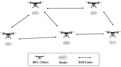
Figure 1: An illustration of DFL systems deployed in wireless D2D networks.

However, DFL encounters several challenges in the training of models. One key issue in DFL is to tackle with data heterogeneity since edge devices often collect data from distinct areas, leading to serious variations in data distributions [5, 6]. Another serious challenge in DFL is the transmission outages caused by the User Datagram Protocol (UDP) widely used in D2D networks. Usually, DFL deployed in D2D networks faces the bottleneck of limited communication resources [7], often relying on the lightweight UDP [3, 4]. However, the use of UDP compromises reliability, resulting in transmission outages and package errors in inter-device communication [3, 4, 8]. Consequently, parameters shared by DFL clients are affected by both data heterogeneity and unreliable D2D links, further deteriorating the convergence and performance of DFL.

Numerous studies have been dedicated to addressing these issues. Some have proposed device scheduling methods [1, 2, 5] to alleviate the impact of data heterogeneity. However, these approaches are tailored to CFL with reliable links. In a study outlined in [3], the DFL system deployed in unreliable D2D networks was optimized by adjusting mixing weights to enhance performance. Nevertheless, this approach overlooked the influence of data heterogeneity. Additionally, the authors of [6] optimized the topology based on their proposed quantity termed neighborhood heterogeneity to enhance the training of DFL models. However, their focus was limited to scenarios with label distribution shift and the deployment of DFL in ideal D2D networks without unreliable links. In summary, existing research has overlooked the theoretical convergence analysis of DFL considering both arbitrary data heterogeneity and unreliable D2D links, thus neglecting the enhancement of DFL training based on these crucial factors.

The main contributions of this paper are as follows: (1) We provide a theoretical analysis of the convergence of DFL with data heterogeneity over unreliable D2D networks. Based on this analysis, we investigate the impact of a new quantity named unreliable links-aware neighborhood discrepancy on the convergence bound of DFL. (2) Motivated by the insights from our theoretical analysis, we develop a novel Topology Learning method considering the Representation Discrepancy and Unreliable Links in DFL, named ToLRDUL, which can enhance the DFL training by minimizing the proposed quantity, further dealing with arbitrary data heterogeneity and unreliable links in DFL. (3) Extensive experiments under feature skew and label skew settings have verified that ToLRDUL outperforms other baselines in both convergence and test accuracy, which is matched with our theoretical findings.

II System Model

In this section, we introduce the details of the considered DFL system. We begin by presenting the decentralized optimization over unreliable D2D networks and then outline the corresponding transmission model. Consistent with [3, 4, 8], we apply the lightweight yet unreliable UDP protocol for DFL, which implies the absence of reliable transmission mechanisms. Consequently, clients discard received packages if they detect errors in packages using error detection codes.

II-A Decentralized optimization over unreliable D2D networks

In this work, we consider the following decentralized optimization objective over an unreliable D2D network of $N$ clients.

$$\min_{\mathbf{w}\in\mathbb{R}^{d}}[f(\mathbf{w}):=\frac{1}{N}\sum_{i=1}^{N}f_{i}(\mathbf{w})],$$ (1)

where $f_{i}(\mathbf{w}):=\mathbb{E}_{Z\sim P^{i}_{Z}}[F(\mathbf{w},Z)]$. $\mathbf{w}\in\mathbb{R}^{d}$ is the model and $F$ is the loss function. $Z=(X,Y)$ is a random variable, where $X$ is the feature and $Y$ is the label. The data heterogeneity is considered, i.e., $P^{i}_{Z}\neq P^{j}_{Z},\forall i\neq j,i,j\in[N]$ and we hypothesize that clients collect data independently.

In the considered DFL system, each client maintains its local models $\mathbf{w}^{i}_{t}$ and shares the local stochastic gradient $\nabla F_{i}(\mathbf{w}^{i}_{t}):=\nabla F(\mathbf{w}^{i}_{t},Z^{i}_{t})\in\mathbb{R}^{d}$ calculated by data $Z^{i}_{t}$ sampled in round $t$ with neighbouring clients based on a specific communication topology over D2D networks to update models. Due to the unreliability of the UDP protocol used in D2D networks, packages may be dropped randomly when received by clients. Following the modeling of [3, 4], the aggregation process is affected by the stochastic reception. Specifically, the reception of gradients is modeled using a Bernoulli random vector $\mathbf{m}_{t}^{i,j}\in\mathbb{R}^{d}$ with its components $\mathbf{m}_{t}^{i,j}(k)\overset{\text{ i.i.d. }}{\sim}Bernoulli(p^{i,j}_{t}),\forall k\in[d]$. Here, $\mathbf{m}_{t}^{i,j}(k)=1$ if the $k$-th component of gradients transmitted by client $j$ is successfully received at client $i$, and $\mathbf{m}_{t}^{i,j}(k)=0$ otherwise. $p^{i,j}_{t}$ thus corresponds to the successful transmission probability from client $j$ to client $i$ in the $t$-th round. Consequently, the update rule of the $i$-th local model follows:

$$\mathbf{w}_{t+1}^{i} =\mathbf{w}_{t}^{i}-\eta_{t}\sum_{j=1}^{N}\theta_{t}^{i,j}\nabla F_{j}(\mathbf{w}^{j}_{t})\odot\mathbf{m}_{t}^{i,j},$$ (2)

where $\eta_{t}$ denotes the learning rate and $\odot$ denotes the element-wise multiplication. The mixing matrix $\boldsymbol{\Theta}_{t}\in\mathbb{R}^{N\times N}=[\theta^{i,j}_{t}]_{N\times N}$ of the topology is a doubly-stochastic matrix, i.e., $\boldsymbol{\Theta}_{t}^{T}=\boldsymbol{\Theta}_{t},\boldsymbol{\Theta}_{t}\mathbf{1}=\mathbf{1}$, where $\mathbf{1}\in\mathbb{R}^{N}$ is an all-ones vector, and $\theta_{t}^{i,j}\neq 0$ only if client $i$ and client $j$ are neighbours.

II-B Transmission model of unreliable D2D networks

In the subsequent analysis, we examine the aforementioned successful transmission probability and the one-round latency for DFL based on the transmission model of the considered D2D network. For our analysis, we assume orthogonal resource allocation among D2D links [9], and thus define the Signal-to-Noise Ratio (SNR) between two connected D2D clients as $\mbox{SNR}_{i,j}(t):=(P_{tx}h^{i,j}_{t}|d^{i,j}_{t}|^{-2})/\sigma^{2}$. Here, $P_{tx}$ is the transmit power and $\sigma^{2}$ is the power of noise. $h^{i,j}_{t}$ denotes the Rayleigh fading, modeled as an independent random variable $h^{i,j}_{t}\sim\exp(1)$ across links and rounds [4]. $|d^{i,j}_{t}|$ indicates the distance between client $i$ and client $j$. Based on this modeling, we define the successful transmission probability as:

$$p^{i,j}_{t} =\mathbb{P}[\mbox{SNR}_{i,j}(t)>\gamma_{th}]=\exp(-\frac{\gamma_{th}\sigma^{2}}{P_{tx}|d_{t}^{i,j}|^{-2}})$$ (3)

where $\gamma_{th}$ denotes the decoding threshold.

In this paper, we focus on the synchronous implementation of DFL and define the transmission latency in one round as:

$$l_{t}:=\max_{i,j\in[N]}\Big{[}\frac{Q}{B\log(1+\frac{P_{tx}h^{i,j}_{t}|d^{i,j}_{t}|^{-2}}{\sigma^{2}})}\Big{]},i\neq j,\theta_{t}^{i,j}\neq 0,$$ (4)

where $Q$ denotes the size of transmitted packages and $B$ is the bandwidth of each link.

III Convergence Analysis

In this section, we conduct the convergence analysis of the average model $\bar{\mathbf{w}}_{t}=\frac{1}{N}\sum_{i=1}^{N}\mathbf{w}^{i}_{t}$ in each round of DFL. Besides, we present a novel neighborhood discrepancy and explore its impact on the derived convergence bound. Our analysis is built upon the following assumptions.

Assumption 1 ($\beta$-smoothness)

There exists a constant $\beta>0$ such that for any $Z$, $\forall\mathbf{w}_{1},\mathbf{w}_{2}$, we have $\big{\|}\nabla F(\mathbf{w}_{1},Z)-\nabla F(\mathbf{w}_{2},Z)\big{\|}\leq\beta\big{\|}\mathbf{w}_{1}-\mathbf{w}_{2}\big{\|}$.

Assumption 2 (Bounded variance)

For any $\mathbf{w}$, the variance of the stochastic gradient is bounded by $\xi$, i.e., $\mathbb{E}_{Z\sim P_{Z}^{i}}\big{\|}\nabla F(\mathbf{w},Z)-\nabla f_{i}(\mathbf{w})\big{\|}^{2}\leq\xi^{2},\forall i\in[N]$.

These assumptions are widely considered in DFL [3, 6, 7]. Next, we introduce a new quantity named unreliable links-aware neighborhood discrepancy and utilize it to derive the convergence bound. Specifically, given $\boldsymbol{\Theta}_{t}$ and $\mathbf{m}_{t}^{i,j},\forall i,j\in[N]$, $\bar{H}$ measuring the average expected distance between the oracle average gradient and the aggregated gradients affected by unreliable links is assumed to be bounded as follows.

Assumption 3 (Bounded unreliable links-aware neighborhood discrepancy)

There exists a constant $\tau>0$, such that for any $[\mathbf{w}_{t}^{i}]_{i\in[N]}$:

$$\bar{H}=\frac{1}{N}\sum_{i=1}^{N}\mathbb{E}\|\sum_{j=1}^{N}\big{(}\theta_{t}^{i,j}\nabla F_{j}(\mathbf{w}^{j}_{t})\odot\mathbf{m}_{t}^{i,j}-\frac{1}{N}\nabla F_{j}(\mathbf{w}^{j}_{t})\big{)}\|^{2}\leq\tau.$$ (5)

Remark 1

Notice that $\bar{H}$ can be further bounded by $\frac{1}{N}\sum_{i=1}^{N}\mathbb{E}\|\frac{1}{N}\sum_{j=1}^{N}\nabla F_{j}(\mathbf{w}^{j}_{t})-\sum_{j=1}^{N}\theta_{t}^{i,j}\nabla F_{j}(\mathbf{w}^{j}_{t})\|^{2}+\frac{1}{N}\sum_{i=1}^{N}\mathbb{E}\|\sum_{j=1}^{N}\big{(}\theta_{t}^{i,j}\nabla F_{j}(\mathbf{w}^{j}_{t})\odot\mathbf{m}_{t}^{i,j}-\theta_{t}^{i,j}\nabla F_{j}(\mathbf{w}^{j}_{t})\big{)}\|^{2}$. The first term measures the neighborhood discrepancy by disregarding the influence of unreliable links, which is commonly assumed to be bounded [6]. Hence, our paper further focuses on scenarios where the second term, which captures the effect of transmission outages on aggregated gradients, remains bounded to support this assumption.

Based on these assumptions, we provide the convergence bound of DFL below and prove it in the appendix.

Theorem 1

Let Assumption 1, 2 and 3 hold. We select the stepsize satisfying $\eta_{t}=\frac{\eta}{\sqrt{T}}\leq\frac{1}{\beta}$, and we have:

$$\min_{0\leq t\leq T}\big{\|}\nabla f(\bar{\mathbf{w}}_{t})\big{\|}^{2} \leq\frac{2(f(\bar{\mathbf{w}}_{0})-f^{*})}{\eta(\sqrt{T}-\beta\eta)}+\frac{\beta\eta+\sqrt{T}}{\sqrt{T}-\beta\eta}\xi^{2}$$ (6)

$$\quad+\frac{(1+\beta^{2}\eta^{2})(\beta\eta+\sqrt{T})}{(\sqrt{T}-\beta\eta)}\tau$$

where $\eta$ is a constant and $f^{*}$ denotes the minimal value of $f$.

Remark 2

Theorem 1 demonstrates that as the upper bound $\tau$ of $\bar{H}$ decreases, the convergence of DFL accelerates, which motivates us to develop a method to learn the topology $\boldsymbol{\Theta}_{t}$ of DFL to approximately minimize $\bar{H}$ for improving the training.

IV Topology Learning

In this section, we derive an upper bound for $\bar{H}$ and formulate a tractable optimization objective for topology learning based on it. Firstly, we introduce another assumption that is widely used in FL [5, 9] to derive this bound.

Assumption 4 (Bounded stochastic gradient)

The expected norm of stochastic gradients is uniformly bounded by a constant $L$, i.e., $\mathbb{E}\|\nabla F_{i}(\mathbf{w}^{i}_{t})\|^{2}\leq L^{2},\forall i\in[N].$

Theorem 2

Let Assumption 4 hold, $\bar{H}$ can be further bounded as follows.

$$\bar{H} \leq\frac{1}{N}\sum_{i=1}^{N}\mathbb{E}\|\sum_{j=1}^{N}\big{(}\theta_{t}^{i,j}\nabla F_{j}(\mathbf{w}^{j}_{t})\odot\mathbf{p}_{t}^{i,j}-\frac{1}{N}\nabla F_{j}(\mathbf{w}^{j}_{t})\big{)}\|^{2}$$ (7)

$$\quad+\frac{dL^{2}}{N}\sum_{i=1}^{N}\sum_{j=1}^{N}(\theta_{t}^{i,j})^{2}p_{i,j}^{t}(1-p_{i,j}^{t}).$$

where $\mathbf{p}_{t}^{i,j}=(p^{i,j}_{t},p^{i,j}_{t},...,p^{i,j}_{t})^{T}\in\mathbb{R}^{d}$. The proof of this theorem is deferred to the appendix.

We now present a viable method to approximate the local gradients in Eq. (7) for formulating a tractable optimization objective. Similar to [10], we employ a probabilistic network to generate the representation $\phi\in\mathbb{R}^{m}(m\ll d)$, with its components $\phi(k)\sim P_{\phi|Z,W}(k),\forall k\in[m]$, to approximate gradients in Eq. (7). Utilizing representations (hidden features) produced by models to approximate the associated stochastic gradients is a proper method, as representations encapsulate essential information about training samples [11]. The representation distributions $\{P^{i}_{\phi|Z,W}\}_{i=1}^{N}$ are modeled as Gaussian distributions in this paper. Specifically, for the $i$-th local model, each component $\phi^{i}(k)$ of the representation $\phi^{i}$ used for label prediction is sampled from a Gaussian distribution $\mathcal{N}\big{(}\phi^{i}(k);\mu^{i}_{t}(k),\sigma^{i}_{t}(k)\big{)}$, where $\mu^{i}_{t}(k)$ and $\sigma^{i}_{t}(k)$ are the corresponding parameters output by the layer preceding the prediction head. For approximating the first term on the right-hand side of Eq. (7), we first define the component-wise average relative entropy for each component $\{\phi^{i}_{t}(k)\}_{i=1}^{N},\forall k\in[m]$ of representations $\{\phi^{i}_{t}\}_{i=1}^{N}$ as follows.

$$\hat{H}^{k}_{t}(\boldsymbol{\Theta}):=\frac{1}{N}\sum_{i=1}^{N}D_{kl}\big{(}\sum_{j=1}^{N}\theta^{i,j}_{t}p_{t}^{i,j}\phi^{j}_{t}(k)\big{\|}\frac{1}{N}\sum_{j=1}^{N}\phi^{j}_{t}(k)\big{)}$$ (8)

With the modeling of Gaussian distributions, we can thus analytically calculate $\hat{H}^{k}_{t}(\boldsymbol{\Theta})$ using the below expression:

$$\hat{H}_{t}^{k}(\boldsymbol{\Theta}) =\frac{1}{N}\sum_{i=1}^{N}\Big{[}\log\frac{\tilde{\sigma}_{t}^{i}(k)}{\bar{\sigma}_{t}(k)}+\frac{\frac{1}{N^{2}}\sum_{j=1}^{N}(\sigma^{j}_{t}(k))^{2}}{2\sum_{j=1}^{N}(\theta^{i,j}p_{t}^{i,j})^{2}(\sigma^{j}_{t}(k))^{2}}$$ (9)

$$\quad+\frac{(\bar{\mu}_{t}(k)-\tilde{\mu}^{i}_{t}(k))^{2}}{2\sum_{j=1}^{N}(\theta^{i,j}p_{t}^{i,j})^{2}(\sigma^{j}_{t}(k))^{2}}-\frac{1}{2}\Big{]}$$

where $\bar{\mu}_{t}(k)=\frac{1}{N}\sum_{j=1}^{N}\mu^{j}_{t}(k)$, $\tilde{\mu}^{i}_{t}(k)=\sum_{j=1}^{N}{\theta}^{i,j}p_{t}^{i,j}\mu^{j}_{t}(k)$, $\bar{\sigma}_{t}(k)=\frac{1}{N}\sum_{j=1}^{N}\sigma^{j}_{t}(k)$, $\tilde{\sigma}_{t}^{i}(k)=\sum_{j=1}^{N}\theta^{i,j}p_{t}^{i,j}\sigma^{j}_{t}(k)$. Referring to [10], we perform the calculation in Eq. (9) for each dimension of representations, and sum them across $m$ dimensions. The sum of $\{\hat{H}_{t}^{k}(\boldsymbol{\Theta})\}_{k=1}^{m}$ serves as an approximation for the term $\frac{1}{N}\sum_{i=1}^{N}\mathbb{E}\|\sum_{j=1}^{N}\big{(}\theta_{t}^{i,j}\nabla F_{j}(\mathbf{w}^{j}_{t})\odot\mathbf{p}_{t}^{i,j}-\frac{1}{N}\nabla F_{j}(\mathbf{w}^{j}_{t})\big{)}\|^{2}$ in Eq. (7), which is justified since relative entropy is well-suited for measuring distribution discrepancy.

Given that the value of $L$ is unknown in practical scenarios, we replace the term $L^{2}$ in Eq. (7) with a hyperparameter $\lambda>0$. Based on the aforementioned results, we formulate the optimization objective for topology learning as follows:

$$\min_{\boldsymbol{\Theta}\in\mathcal{S}}\Big{\{}g(\boldsymbol{\Theta}):=\sum_{k=1}^{m}\hat{H}^{k}_{t}(\boldsymbol{\Theta})+\frac{d\lambda}{N}\sum_{i,j=1}^{N}(\theta^{i,j})^{2}p_{t}^{i,j}(1-p_{t}^{i,j})\Big{\}},$$ (10)

where $\mathcal{S}$ is a set of doubly-stochastic matrix. The underlying idea of this optimization objective is to learn a topology both enabling aggregated representations affected by outages to approximate the oracle average representation, and mitigating the influence from the variance of unreliable links.

Input: Initialization $\boldsymbol{\Theta}_{0}=\mathbf{I}$ and hyperparameters $\lambda\geq 0,K<T,K\in\mathbb{N}^{+}$.

1 for round $t\in[T]$  do

2      

3      for client $i\in[N]$ in parallel do

4             $\boldsymbol{\Theta}_{t}=\boldsymbol{\Theta}_{t-1}$;

5             if $t$ mod $K$=0 then

6                   Exchange encrypted information to attain $(\boldsymbol{\mu}_{t},\boldsymbol{\sigma}_{t})$ and $\mathbf{P}_{t}$ via all-reduce;

7                   $\boldsymbol{\hat{\Theta}}\leftarrow\mbox{Frank-Wolfe}\big{(}g(\boldsymbol{\Theta}_{t},(\boldsymbol{\mu}_{t},\boldsymbol{\sigma}_{t}),\mathbf{P}_{t},\lambda)\big{)}$;

8                   $\boldsymbol{\Theta}_{t}=\boldsymbol{\hat{\Theta}}$;

9                  

10             end if

11            

12            $\mathbf{w}_{t+1}^{i}=\mathbf{w}_{t}^{i}-\eta_{t}\sum_{j=1}^{N}\theta_{t}^{i,j}\nabla F(\mathbf{w}_{t}^{j},Z_{t}^{j})\odot\mathbf{m}_{t}^{i,j}$;

13            

14       end for

15      

16 end for

Algorithm 1 Topology Learning considering the Representation Discrepancy and Unreliable Links for DFL

Drawing from the method outlined in [6], we adopt the Frank-Wolfe (FW) algorithm to find the approximate solution of Eq. (10), which is well-suited for learning a sparse parameter over convex hulls of finite set of atoms [6]. In our context, $\mathcal{S}$ corresponds to the convex hull of the set of all permutation matrices [6], enabling our approach to learn a sparse topology including both edges and their associated mixing weights. To execute this approach, clients encrypt and exchange packages every $K$ round. These packages encompass locations used for calculating $\mathbf{P}_{t}=[p_{t}^{i,j}]_{N\times N}$, as well as $(\boldsymbol{\mu}_{t},\boldsymbol{\sigma}_{t})$ denoting the parameters of all the Gaussian distributions. This scheme incurs low communication costs since the lower dimension of representations compared to gradients and lower communication frequency. Clients can thus utilize reliable protocols to exchange these packages without experiencing outages. The detailed workflow of this method is described in Algorithm 1.

V Numerical Results

In this section, we conduct numerical experiments to evaluate the effectiveness of the proposed ToLRDUL. We provide the details of the transmission model used in the considered D2D networks below. The bandwidth is set to $5$MHz, the transmission power $P_{tx}$ is set to $10$dBm and the noise power $\sigma^{2}$ is set to $-169$dBm. The decoding threshold $\gamma_{th}$ is set to $0$dB. We deploy the D2D network in a region of $1000\times 1000$ $m^{2}$ with $100$ randomly distributed clients participating in DFL. The size of transmitted packages is set to $1.2$MB.

We utilize CNN as the backbone model. Clients perform SGD with a mini-batch size of $128$ and a learning rate of $0.1$. We employ two widely used variants of the CIFAR-10 dataset: Dirichlet CIFAR-10 and Rotated CIFAR-10 [12]. These two variants are chosen to model label skew and feature skew settings respectively. For Dirichlet CIFAR-10, we set the parameter of Dirichlet distribution to $0.1$. For Rotated CIFAR-10, we rotate images clockwise by $3.6^{\circ}$ for each time and distribute them to $100$ clients one by one. We test the average model $\bar{\mathbf{w}}_{t}$ on the global test set following the same distribution as that of all the clients. We compare our method with STL-FW proposed in [6], which only leverages the label distribution shift to learn the topology. Besides, we set the random $r$-regular graph [6] and fully-connected graph as baselines, with uniform weights for all activated links. The hyperparameter $\lambda$ and $K$ of ToLRDUL are set to $0.001$ and $3$ respectively.

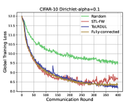
(a) Training loss

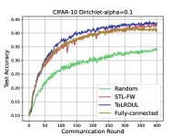
(b) Test accuracy

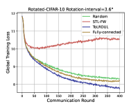
(c) Training loss

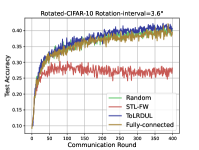
(d) Test accuracy

Figure 2: Convergence analysis of DFL with ToLRDUL and other baselines on label-skew and feature skew CIFAR-10.

We begin by analyzing the convergence of ToLRDUL and other baselines. We fix the degree $r$ of nodes to be $2$ in this analysis. As shown in Fig. 2 (a) and (b), ToLRDUL demonstrates faster and more stable convergence, achieving the highest test accuracy on Dirichlet CIFAR-10 after $400$ rounds. On the contrary, STL-FW neglects the impact of unreliable links, resulting in unstable convergence. Furthermore, the fully-connected graph performs worse than ToLRDUL due to an excessive number of unreliable links among connected clients. This leads to frequent transmission outages, which hinder the training of the model. Next, we turn our attention to the convergence analysis on Rotated CIFAR-10 in Fig. 2 (c) and (d). Similarly, ToLRDUL outperforms baselines in both convergence and test accuracy. Notably, STL-FW performs even worse than the random $r$-regular graph on Rotated CIFAR-10 since it fails to employ the feature distribution discrepancy to learn the topology when confronted with the challenge of feature distribution skew.

TABLE I: Dirichlet CIFAR-10 after $300$ communication rounds

Method Test accuracy Transmission latency $r$=2 $r$=4 $r$=10 $r$=2 $r$=4 $r$=10 ToLRDUL (ours) 43.42% 43.43% 43.77% 44.88s 56.46s 65.73s STL-FW 41.10% 42.88% 41.92% 62.38s 74.45s 85.70s Random 33.16% 42.61% 41.77% 61.83s 73.62s 85.30s Fully-connected 41.61% 41.61% 41.61% 92.13s 92.13s 92.13s

TABLE II: Rotated CIFAR-10 after $300$ communication rounds

Method Test accuracy Transmission latency $r$=2 $r$=4 $r$=10 $r$=2 $r$=4 $r$=10 ToLRDUL (ours) 41.40% 41.70% 41.50% 45.23s 56.69s 66.22s STL-FW 30.30% 31.70% 40.60% 59.80s 71.80s 82.34s Random 40.20% 41.20% 40.50% 60.81s 72.52s 83.34s Fully-connected 39.10% 39.10% 39.10% 90.50s 90.50s 90.50s

Then we investigate the effect of the degree $r$ of nodes on two variants of CIFAR-10. The results are summarized in Table I and Table II. We find that increasing the value of $r$ leads to an enlargement of the transmission latency $l_{t}$ since activating more links may result in a higher number of unreliable links. Denser topologies result in larger values of $l_{t}$, aligning with our intuition. Besides, an excess of activated links in fully-connected graph cause severe package errors and thus degrade the test accuracy. Notice that ToLRDUL achieves the lowest latency and the highest test accuracy under all three settings since it utilizes both data heterogeneity and channel conditions to learn the topology for performing DFL better.

VI Conclusion

In this paper, we present a theoretical convergence analysis for DFL with data heterogeneity over unreliable D2D networks. Furthermore, we introduce a novel quantity called unreliable links-aware neighborhood discrepancy and show its influence on the derived convergence bound. Building upon this observation, we develop a topology learning method named ToLRDUL to approximately minimize the proposed quantity for improving the convergence and performance of DFL. To validate the effectiveness of our approach, we conduct extensive experiments that confirm its superiority over other baselines, in accordance with our theoretical findings.

-A Proof of Theorem 1

Proof 1

According to Assumption 1, we have:

$$f(\bar{\mathbf{w}}_{t+1}) \leq f(\bar{\mathbf{w}}_{t})\underbrace{-\mathbb{E}\big{<}\nabla f(\bar{\mathbf{w}}_{t}),\sum_{i,j=1}^{N}\frac{\eta_{t}\theta^{i,j}_{t}}{N}\nabla F_{j}(\mathbf{w}_{t}^{j})\odot\mathbf{m}_{t}^{i,j}\big{>}}_{T_{1}}$$ (11)

$$\quad+\underbrace{\frac{\beta}{2}\mathbb{E}\big{\|}\frac{\eta_{t}}{N}\sum_{i,j=1}^{N}\theta^{i,j}_{t}\nabla F_{j}(\mathbf{w}_{t}^{j})\odot\mathbf{m}_{t}^{i,j}\big{\|}^{2}}_{T_{2}}.$$

Next, we proceed to add and subtract the term $\eta_{t}\nabla f(\bar{\mathbf{w}}_{t})$ in $T_{1}$, and we can thus convert $T_{1}$ into: $-\eta_{t}\big{\|}\nabla f(\bar{\mathbf{w}}_{t})\big{\|}^{2}+\frac{\eta_{t}}{N}\mathbb{E}\sum_{i=1}^{N}\big{<}\nabla f(\bar{\mathbf{w}}_{t}),\nabla f(\bar{\mathbf{w}}_{t})-\sum_{j=1}^{N}\theta^{i,j}_{t}\nabla F_{j}(\mathbf{w}_{t}^{j})\odot\mathbf{m}_{t}^{i,j}\big{>}$.

We then upper-bound this term for bounding $T_{1}$:

$$T_{1} \leq-\frac{\eta_{t}}{2}\big{\|}\nabla f(\bar{\mathbf{w}}_{t})\big{\|}^{2}+\frac{\eta_{t}}{2N}\sum_{i=1}^{N}\mathbb{E}\big{\|}\nabla f(\bar{\mathbf{w}}_{t})$$ (12)

$$+\frac{1}{N}\sum_{j=1}^{N}\big{(}\nabla f_{j}(\mathbf{w}_{t}^{j})-\nabla f_{j}(\mathbf{w}_{t}^{j})-\nabla F_{j}(\mathbf{w}_{t}^{j})\big{)}\big{\|}^{2}$$

$$+\frac{\eta_{t}}{2N}\sum_{i=1}^{N}\mathbb{E}\big{\|}\sum_{j=1}^{N}\big{(}\frac{1}{N}\nabla F_{j}(\mathbf{w}_{t}^{j})-\theta^{i,j}_{t}\nabla F_{j}(\mathbf{w}_{t}^{j})\odot\mathbf{m}_{t}^{i,j}\big{)}\big{\|}^{2}$$

$$\leq-\frac{\eta_{t}}{2}\big{\|}\nabla f(\bar{\mathbf{w}}_{t})\big{\|}^{2}+\frac{\eta_{t}\beta^{2}}{2N}\sum_{i=1}^{N}\big{\|}\bar{\mathbf{w}}_{t}-\mathbf{w}_{t}^{i}\big{\|}^{2}+\frac{\eta_{t}(\xi^{2}+\tau)}{2},$$

where $\nabla f(\mathbf{\bar{W}}_{t})=[\nabla f(\bar{\mathbf{w}}_{t}),\nabla f(\bar{\mathbf{w}}_{t}),...,\nabla f(\bar{\mathbf{w}}_{t})]\in\mathbb{R}^{d\times N}$. The last inequality holds since Assumption 1, 2 and 3.

Then we concentrate on bounding $T_{2}$.

$$T_{2} \leq\frac{\beta\eta_{t}^{2}}{2N}\sum_{i=1}^{N}\mathbb{E}\big{\|}\sum_{j=1}^{N}\big{(}\theta^{i,j}_{t}\nabla F_{j}(\mathbf{w}_{t}^{j})\odot\mathbf{m}_{t}^{i,j}-\frac{1}{N}\nabla F_{j}(\mathbf{w}_{t}^{j})\big{)}$$ (13)

$$\quad+\frac{1}{N}\sum_{j=1}^{N}\big{(}\nabla F_{j}(\mathbf{w}_{t}^{j})-\nabla f_{j}(\mathbf{w}_{t}^{j})+\nabla f_{j}(\mathbf{w}_{t}^{j})$$

$$\quad\quad-\nabla f_{j}(\bar{\mathbf{w}}_{t})+\nabla f_{j}(\bar{\mathbf{w}}_{t})\big{)}\big{\|}^{2}$$

$$\leq\frac{\beta\eta_{t}^{2}}{2}(\tau+\xi^{2}+\big{\|}\nabla f(\bar{\mathbf{w}}_{t})\big{\|}^{2})+\frac{\beta^{3}\eta_{t}^{2}}{2N}\sum_{i=1}^{N}\big{\|}\bar{\mathbf{w}}_{t}-\mathbf{w}_{t}^{i}\big{\|}^{2}.$$

The term $T_{3}:=\frac{1}{N}\sum_{i=1}^{N}\mathbb{E}\big{\|}\bar{\mathbf{w}}_{t}-\mathbf{w}_{t}^{i}\big{\|}^{2}$ can be bounded as:

$$T_{3} \leq\frac{1}{N}\sum_{i=1}^{N}\mathbb{E}\big{\|}\bar{\mathbf{w}}_{t-1}-\mathbf{w}_{t-1}^{i}\big{\|}^{2}+\frac{\eta_{t-1}^{2}}{N}\sum_{i=1}^{N}\big{[}(1+\frac{1}{N})$$ (14)

$$\mathbb{E}\big{\|}\sum_{j=1}^{N}\big{(}\frac{1}{N}\nabla F_{j}(\mathbf{w}_{t-1}^{j})-\theta_{t-1}^{i,j}\nabla F_{j}(\mathbf{w}_{t-1}^{j})\odot\mathbf{m}^{i,j}_{t-1}\big{)}\big{\|}^{2}\big{]}$$

$$\leq\frac{1}{N}\sum_{i=1}^{N}\mathbb{E}\big{\|}\bar{\mathbf{w}}_{t-1}-\mathbf{w}_{t-1}^{i}\big{\|}^{2}+2\eta_{t-1}^{2}\tau$$

$$\leq\frac{1}{N}\sum_{i=1}^{N}\mathbb{E}\big{\|}\bar{\mathbf{w}}_{0}-\mathbf{w}_{0}^{i}\big{\|}^{2}+2\tau\sum_{l=1}^{t}\eta_{l-1}^{2}.$$

Notice that $\bar{\mathbf{w}}_{0}=\mathbf{w}_{0}^{i},\forall i\in[N]$, the term $\frac{1}{N}\sum_{i=1}^{N}\mathbb{E}\big{\|}\bar{\mathbf{w}}_{t}-\mathbf{w}_{t}^{i}\big{\|}^{2}$ can thus be bounded by $2\tau\sum_{l=1}^{t}\eta_{l-1}^{2}$.

To incorporate the above results and select the stepsize satisfying $\eta_{t}=\frac{\eta}{\sqrt{T}}\leq\frac{1}{\beta}$, we can immediately derive the below convergence bound of the considered DFL:

$$\min_{0\leq t\leq T}\big{\|}\nabla f(\bar{\mathbf{w}}_{t})\big{\|}^{2} \leq\frac{2(f_{0}-f^{*})}{\eta(\sqrt{T}-\beta\eta)}+\frac{\beta\eta+\sqrt{T}}{\sqrt{T}-\beta\eta}\xi^{2}$$ (15)

$$\quad+\frac{(1+\beta^{2}\eta^{2})(\beta\eta+\sqrt{T})}{(\sqrt{T}-\beta\eta)}\tau.$$

-B Proof of Theorem 2

Proof 2

Based on Assumption 4, $\bar{H}$ can be bounded as:

$$\bar{H} \leq\frac{1}{N}\sum_{i=1}^{N}\mathbb{E}\|\sum_{j=1}^{N}\big{(}\theta_{t}^{i,j}\nabla F_{j}(\mathbf{w}^{j}_{t})\odot\mathbf{p}_{t}^{i,j}-\frac{1}{N}\nabla F_{j}(\mathbf{w}^{j}_{t})\big{)}\|^{2}$$ (16)

$$\quad+\frac{1}{N}\sum_{i=1}^{N}\mathbb{E}\|\sum_{j=1}^{N}\theta_{t}^{i,j}\nabla F_{j}(\mathbf{w}^{j}_{t})\odot(\mathbf{p}_{t}^{i,j}-\mathbf{m}_{t}^{i,j})\|^{2}$$

$$\leq\frac{1}{N}\sum_{i=1}^{N}\mathbb{E}\|\sum_{j=1}^{N}\big{(}\theta_{t}^{i,j}\nabla F_{j}(\mathbf{w}^{j}_{t})\odot\mathbf{p}_{t}^{i,j}-\frac{1}{N}\nabla F_{j}(\mathbf{w}^{j}_{t})\big{)}\|^{2}$$

$$\quad+\frac{dL^{2}}{N}\sum_{i=1}^{N}\sum_{j=1}^{N}(\theta_{t}^{i,j})^{2}p_{i,j}^{t}(1-p_{i,j}^{t}),$$

where the last inequality holds since the expected square norm $\mathbb{E}\|\mathbf{p}_{t}^{i,j}-\mathbf{m}_{t}^{i,j}\|^{2}=dp_{i,j}^{t}(1-p_{i,j}^{t})$.

References

• [1] T. Yin, L. Li, W. Lin, T. Ni, Y. Liu, H. Xu, and Z. Han, “Joint client scheduling and wireless resource allocation for heterogeneous federated edge learning with non-iid data,” IEEE Transactions on Vehicular Technology, pp. 1–13, 2023.
• [2] H. Zhu, J. Kuang, M. Yang, and H. Qian, “Client selection with staleness compensation in asynchronous federated learning,” IEEE Transactions on Vehicular Technology, vol. 72, no. 3, pp. 4124–4129, 2023.
• [3] H. Ye, L. Liang, and G. Y. Li, “Decentralized federated learning with unreliable communications,” IEEE J. Sel. Top. Signal Process., vol. 16, no. 3, pp. 487–500, 2022.
• [4] Z. Wu, X. Wu, and Y. Long, “Joint scheduling and robust aggregation for federated localization over unreliable wireless d2d networks,” IEEE Transactions on Network and Service Management, 2022.
• [5] Z. Chen, W. Yi, and A. Nallanathan, “Exploring representativity in device scheduling for wireless federated learning,” IEEE Transactions on Wireless Communications, 2023.
• [6] B. L. Bars, A. Bellet, M. Tommasi, E. Lavoie, and A. Kermarrec, “Refined convergence and topology learning for decentralized SGD with heterogeneous data,” in AISTATS, vol. 206 of Proceedings of Machine Learning Research, pp. 1672–1702, PMLR, 2023.
• [7] W. Liu, L. Chen, and W. Zhang, “Decentralized federated learning: Balancing communication and computing costs,” IEEE Trans. Signal Inf. Process. over Networks, vol. 8, pp. 131–143, 2022.
• [8] Z. Yan and D. Li, “Performance analysis for resource constrained decentralized federated learning over wireless networks,” arXiv preprint arXiv:2308.06496, 2023.
• [9] C. Hu, Z. Chen, and E. G. Larsson, “Scheduling and aggregation design for asynchronous federated learning over wireless networks,” IEEE J. Sel. Areas Commun., vol. 41, no. 4, pp. 874–886, 2023.
• [10] A. T. Nguyen, P. H. S. Torr, and S. N. Lim, “Fedsr: A simple and effective domain generalization method for federated learning,” in NeurIPS, 2022.
• [11] D. A. Roberts, S. Yaida, and B. Hanin, The principles of deep learning theory. Cambridge University Press Cambridge, MA, USA, 2022.
• [12] A. B. de Luca, G. Zhang, X. Chen, and Y. Yu, “Mitigating data heterogeneity in federated learning with data augmentation,” arXiv preprint arXiv:2206.09979, 2022.