Thermodynamic topology of 4D Euler-Heisenberg-AdS black hole in different ensembles

Abstract

We study the thermodynamic topology of 4D Euler-Heisenberg-AdS (EHAdS) black hole and higher-order QED corrected Euler-Heisenberg-AdS black hole in different ensembles using generalized off-shell free energy. In this approach, black holes are viewed as defects in the thermodynamic space. We work in two ensembles: canonical ensemble in which the charge is kept fixed and grand canonical ensemble in which the conjugate potential $\phi_{e}$ is kept fixed. In each case, the local and global topology of the thermodynamic space is investigated via the computation of winding numbers at the defects. For 4D Euler-Heisenberg-AdS black hole in canonical ensemble, the topological class is found to be different depending on the Euler-Heisenberg (EH) parameter $a$. The topological numbers for $a<0$ and $a>0$ cases are found to be $W=+1$ and $W=0$ respectively. The topological number is found to be independent of the variation in pressure $P$ and charge $Q$ of the black hole. With the introduction of higher order QED correction, the difference in the topological class of 4D EHAdS black hole with the sign of $a$ is observed to go away.The topological number in this case is found to be $W=+1$ irrespective of the values of $a$, $P$ and $Q$. In the grand canonical ensemble, the topological number for both EHAdS and higher order QED corrected EHAdS black hole is found to be $W=0$, independent of the values of $P$, $\phi_{e}$ and $a$. Therefore, we infer that the topological class of both 4D EHAdS black hole and higher order QED corrected EHAdS black hole is ensemble dependent. Moreover, in the canonical ensemble, higher order QED correction alters the topological class of the black hole for positive values of EH parameter $a$. In the grand canonical ensemble, the higher order corrections do not change the thermodynamic topology of the black hole.

Naba Jyoti Gogoi¹ Prabwal Phukon^1,2

I Introduction

Since the realization of black holes as thermodynamic systems, it has been a very active area of research in physics producing many foundational and interesting results [1, 2, 3, 4, 5, 6, 7, 8, 9, 10, 11, 12, 13, 14, 15]. Of late, black hole thermodynamics has been rigorously studied in the extended thermodynamic space where the cosmological constant $\Lambda$ is incorporated in the Smarr formula as pressure $P$ [16, 18, 17, 19]. The thermodynamics and phase transition of various anti-de Sitter (AdS) black holes have been studied in this space [20, 21, 22, 23, 24, 25, 26, 27, 28, 29, 30, 31, 32, 33].

Another important contribution to this area of research is the topological approach of black hole thermodynamics. The idea was proposed in [34] which is a simple and straightforward method adopted from Duan’s topological $\phi$-mapping theory[35]. Two formerly unknown critical points: novel and conventional, are proposed and are endowed with topological charges $+1$ and $-1$ respectively. The conventional critical point is related to the first-order phase transition of a black hole system. Following this, another important concept is proposed in [36] where, using the generalized off-shell free energy, the black hole systems are viewed as thermodynamic defects in the parameter space. In this approach, the generalized free energy expression is used which is given as

$$\mathcal{F}=E-\frac{S}{\tau},$$ (1)

where, $E$ and $S$ are the energy and entropy of the black hole. Also, $\tau$ is the inverse of temperature. The vector function is calculated as $\phi=(\partial_{r_{+}}\mathcal{F},-\cot\Theta\csc\Theta)$. The $\Theta$ parameter is added for convenience. The condition $\Theta=\pi/2$ gives the zero points of $\phi$. Around each zero point contour $C$ parametrized by $\vartheta\in(0,2\pi)$ is drawn which is defined as [34]:

$$\begin{cases}&r_{+}=a\cos\vartheta+r_{0},\\ &\theta=b\sin\vartheta+\frac{\pi}{2}.\end{cases}$$ (2)

The winding numbers are calculated by $w=\frac{1}{2\pi}\Omega(2\pi)$ where the deflection of vector field $n$ along the contour $C$ is

$$\Omega(\vartheta)=\int_{0}^{\vartheta}\epsilon_{ab}n^{a}\partial_{\vartheta}n^{b}d\vartheta.$$ (3)

The winding numbers reveal the local topological behaviour at the defects and the topological number $W$, which is the sum of the winding numbers, provides information about the global topological behaviour. The study of thermodynamic topology by now has been extended to a number of black hole systems [37, 38, 39, 40, 41, 42, 43, 44, 45, 46, 47, 48, 49, 50, 51, 52, 53, 54, 55, 56, 57, 58, 59, 60, 61, 62].

Recently, an alternative method of calculating the winding numbers is proposed by Fang, Jiang and Zhang which uses the concept of residue theorem [63]. This method suggest a complex function $\mathcal{R}(z)$ which is defined as

$$\mathcal{R}(z)\equiv\frac{1}{\tau-\mathcal{G}(z)}.$$ (4)

Here, $\tau=\mathcal{G}(r_{+})$ is calculated from the generalized free energy using the condition $\partial_{r_{+}}\mathcal{F}=0$. Then, the event horizon radius $r_{+}$ is replaced by a complex variable $z$. With such consideration, the defect points can be represented by the isolated singular points $z_{i}$ of $\mathcal{R}(z)$ on the complex plane $\mathbb{C}$ defined by complex variable $z=x+iy$ with $x,y\in\mathbb{R}$. Contour $C_{i}$ can be drawn enclosing each real singular point $z_{i}=z_{1},z_{2},...,z_{m}$. The complex function $\mathcal{R}(z)$ is then analytic on and within the contour except for these singular points. Using the Residue theorem, integral of $\mathcal{R}(z)$ is calculated along each contour $C_{i}$

$$\oint_{C}\frac{\mathcal{R}(z)}{2\pi i}dz=\sum_{k=1}^{m}\text{Res}[\mathcal{R}(z_{k})].$$ (5)

Then, the winding number can be calculated as

$$w_{i}=\frac{\text{Res}\mathcal{R}(z_{i})}{|\text{Res}\mathcal{R}(z_{i})}|=\text{Sgn}[\text{Res}\mathcal{R}(z_{i})],$$ (6)

where, $\text{Sgn}(x)$ is the sign function which is zero for $x=0$ and for any real $x$, returns its sign. From the Cauchy-Goursat theorem, it is possible to calculate the integral of $\mathcal{R}(z)$ along an exterior contour which is over the interior contours that enclose the singular points. Mathematically,

$$\oint_{C}\mathcal{R}(z)dz=\sum_{i}\oint_{C_{i}}\mathcal{R}(z)dz.$$ (7)

This permits the calculation of the topological number as

$$W=\sum_{i}w_{i}.$$ (8)

Various black hole systems have been studied using this approach [64, 65]. The results are found to be consistent with the results obtained by the topological current method [63].

In this work, we study the thermodynamic topology of 4D Euler-Heisenberg-AdS black hole using the generalized off-shell free energy. The winding number as well as the topological numbers are calculated to analyse the local and global topological properties. We mainly focus on how different parameters of aforementioned black hole system affects the thermodynamic topology. Then, we extend our work to the higher-order QED corrected Euler-Heisenberg-AdS black hole and study the impact on the higher order correction in the thermodynamic topology. We perform our analysis in two ensembles: fixed charged (canonical) and fixed potential (grand canonical) ensemble.

It is to be noted that the thermodynamic topology of 4D Euler-Heisenberg AdS black hole in fixed charged ensemble has been previously studied in [71] using Duan’s topological $\phi$-mapping theory. In this work, we have used a different method namely the generalized off-shell free energy method. Moreover, we conduct our study in not only the fixed charged ensemble but also the fixed potential ensemble. By doing this, we want to see how a change of ensemble affects the thermodynamic topology of this black hole. In addition to this, we also consider higher order QED corrected version of 4D EHAdS black hole. Our aim is to understand whether the higher order QED corrections changes the thermodynamic topology of the black hole or not.

This paper is organized as follows. We begin with the study of 4D Euler-Heisenberg-AdS black hole in canonical ensemble in section II. This is followed by, section III in which we study the higher-order QED corrected Euler-Heisenberg-AdS black hole in canonical ensemble. Next, in section IV and section V, we study the Euler-Heisenberg-AdS black hole and the higher-order QED corrected Euler-Heisenberg-AdS black hole in the grand canonical ensemble respectively. Finally, we summarized our results in the section VI.

II 4D Euler-Heisenberg-AdS black hole in canonical ensemble

The 4D Euler-Heisenberg-AdS (EHAdS) black hole is a solution of the Einstein-Maxwell equations which has a negative cosmological constant and a nonlinear electromagnetic field [66, 67] The nonlinear electrodynamic field arises from quantum electrodynamics corrections to the Maxwell theory and it is described by the Euler-Heisenberg Lagrangian. The metric of a static and spherically symmetric 4D EHAdS black hole is given by

$$ds^{2}=-f(r)dt^{2}+\frac{dr^{2}}{f(r)}+r^{2}d\Omega^{2}.$$ (9)

Here,

$$f(r)=1-\frac{2M}{r}+\frac{Q^{2}}{r^{2}}-\frac{\Lambda r^{2}}{3}-\frac{aQ^{4}}{20r^{6}},$$ (10)

where $M$ is the mass, $Q$ is the electric charge, $\Lambda$ is the cosmological constant, and $a$ is the Euler-Heisenberg (EH) parameter. The parameter $a$ is proportional to the square of the fine structure constant $\alpha$ and inversely proportional to the fourth power of the electron mass $m$:

$$a=\frac{8\alpha^{2}}{45m^{4}},$$ (11)

where we choose $c=\hbar=1$. The EH parameter measures the strength of the quantum electrodynamics (QED) correction to the Maxwell field.

The thermodynamics and phase transitions of this black hole have already been studied in a number of remarkable works [67, 68]. It has been found that the EH parameter $a$ affects the thermodynamics and phase transition of the Euler-Heisenberg-AdS black hole. Depending on the value of a, the black hole can exhibit interesting phase transition behaviors. Such as, for $a<0$, the black hole can undergo a first-order phase transition between small and large black holes, similar to the van der Waals system. For $0\leq a\leq\frac{32}{7}Q^{2}$, there is reentrant phase transition. For $a>\frac{32}{7}Q^{2}$, there is no phase transition [69].

The cosmological constant can be represented in terms of pressure as $\Lambda=-8\pi P$. With this definition of pressure the relevant thermodynamic parameters such as entropy, energy and temperature of the black hole are respectively given as

$$S=\pi r_{+}^{2},$$ (12)

$$E=M=\frac{r_{+}}{2}+\frac{4}{3}\pi Pr_{+}^{3}+\frac{Q^{2}}{2r_{+}}-\frac{aQ^{4}}{40r_{+}^{5}},$$ (13)

and

$$T=\frac{aQ^{4}+32\pi Pr_{+}^{8}-4Q^{2}r_{+}^{4}+4r_{+}^{6}}{16\pi r_{+}^{7}}.$$ (14)

The generalized free energy is given as

$$\mathcal{F} =E-\frac{S}{\tau}$$ (15)

$$=\frac{4}{3}\pi Pr_{+}^{3}+\frac{Q^{2}}{2r_{+}}-\frac{aQ^{4}}{40r_{+}^{5}}-\frac{\pi r_{+}^{2}}{\tau}+\frac{r_{+}}{2},$$

where, $\tau$ is the inverse of temperature. For the Duan’s $\phi$ mapping theory, the vector field is defind as

$$\phi=(\partial_{r_{+}}\mathcal{F},-\cot\Theta\csc\Theta),$$ (16)

where, $\Theta$ is added here for convenience and $0\leq\Theta\leq\pi$. Using $\partial_{r_{+}}\mathcal{F}=0$, we calculate the curve of zero points of $\phi$:

$$\tau=\frac{16\pi r_{+}^{7}}{aQ^{4}+32\pi Pr_{+}^{8}-4Q^{2}r_{+}^{4}+4r_{+}^{6}}.$$ (17)

Now, from (4), we define the complex function as

$$\mathcal{R}_{EH}(z)=\frac{aQ^{4}+32\pi Pz^{8}-4Q^{2}z^{4}+4z^{6}}{aQ^{4}\tau+32\pi P\tau z^{8}-4Q^{2}\tau z^{4}+4\tau z^{6}-16\pi z^{7}}.$$ (18)

We take the denominator of the equation and define a polynomial function $\mathcal{A}(z)$ as

$$\mathcal{A}(z)=aQ^{4}\tau+32\pi P\tau z^{8}-4Q^{2}\tau z^{4}+4\tau z^{6}-16\pi z^{7}.$$ (19)

Using $\mathcal{A}(z)$, we can calculate the poles of $\mathcal{R}(z)_{EH}$.

II.1 For negative $a$

We first consider the case of the negative EH parameter $(a<0)$. For such a case, variations of $\tau(r_{+})$ for different parameters are shown in Figure 1.

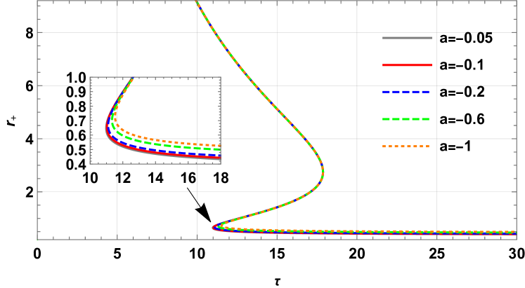
(a) Zero points of $\phi$ for different negative values of $a$. Here $P=0.005$ and $Q=0.36$.

(b) Zero points of $\phi$ for different values of $Q$. Here $a=-0.1$ and $P=0.005$

(c) Zero points of $\phi$ for different values of $P$. Here $a=-0.1$ and $Q=0.36$

Figure 1: Zero points of $\phi$ in $r_{+}$ vs $\tau$ plane with different parameter variations for EHAdS black hole in canonical ensemble (for negative $a$).

For a set of parameters $(a,P,Q)=(-0.1,0.005,0.36)$, we proceed to calculate the poles of (18) by substituting these values in the polynomial function (19). This provides

$$\mathcal{A}(z)=-0.00167962\tau+0.502655\tau z^{8}+4\tau z^{6}-0.5184\tau z^{4}-16\pi z^{7}.$$ (20)

A graphical representation in Figure 2 shows the roots of the polynomial function $\mathcal{A}(z)$ for different values of $\tau$. For example, with $\tau=15$, we have three positive real roots of $\mathcal{A}(z)$ which are $z_{1}=0.466388,~{}z_{2}=1.41858,~{}z_{3}=5.12015$.

Figure 2: Plot of the polynomial function $\mathcal{A}(z)$ for $\tau=10,~{}15,\text{and}~{}25$. The black dots represents the roots for $\tau=15$.

Using residue theorem we can calculate the winding numbers. For $z_{1},~{}z_{2}$ and $z_{3}$ the winding numbers are

$$w_{1}=+1,\quad w_{2}=-1,\quad w_{3}=+1.$$ (21)

The topological number is hence $W=w_{1}+w_{2}+w_{3}=+1$. In the same parameter configuration, for $\tau=10$ and $\tau=25$ we find $w=+1$ for each value of $\tau$. This imply that the topological number, $W$, is also $+1$. We also calculate the winding number as well as the topological number for different variations of parameters and the results are shown in Table 1. The results shows that the topological number $W=+1$ is independent of the parameter variation.

EHAdS black hole
Parameters			$\tau$	Winding number	Topological number
P	Q	a
0.005	0.36	-0.1	10	$w_{1}=+1$	$W=+1$
			15	$w_{1}=+1$ $w_{2}=-1$ $w_{3}=+1$	$W=+1$
			25	$w_{1}=+1$	$W=+1$
0.005	0.36	-0.6	10	$w_{1}=+1$	$W=+1$
			15	$w_{1}=+1$ $w_{2}=-1$ $w_{3}=+1$	$W=+1$
			25	$w_{1}=+1$	$W=+1$
0.005	0.1	-0.1	5	$w_{1}=+1$ $w_{2}=-1$ $w_{3}=+1$	$W=+1$
			10	$w_{1}=+1$ $w_{2}=-1$ $w_{3}=+1$	$W=+1$
			15	$w_{1}=+1$ $w_{2}=-1$ $w_{3}=+1$	$W=+1$
0.005	0.9	-0.1	10	$w_{1}=+1$	$W=+1$
			15	$w_{1}=+1$	$W=+1$
			20	$w_{1}=+1$	$W=+1$
0.2	0.36	-0.1	4	$w_{1}=+1$	$W=+1$
			8	$w_{1}=+1$	$W=+1$
			12	$w_{1}=+1$	$W=+1$

Table 1: Winding numbers and Topological numbers for EHAdS black hole in canonical ensemble for negative $a$

II.2 For positive $a$

Here, we consider the EH parameter $a$ to be positive, i.e., $a>0$. For this case, the zero points of $\phi$ are shown in Figure 3 for a range different constant parameters. The figures are plotted using (17). From the figure we observe either $2$ or $4$ different branches of the $\tau(r_{+})$ curve.

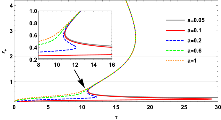
(a) Zero points of $\phi$ for different positive values of $a$. Here $P=0.005$ and $Q=0.36$.

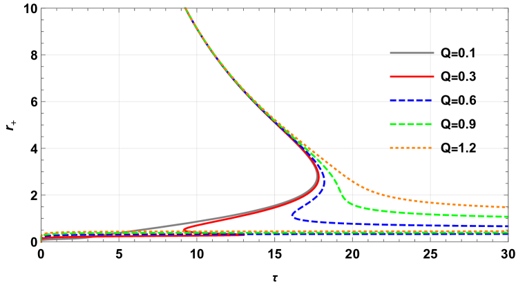
(b) Zero points of $\phi$ for different values of $Q$. Here $a=0.1$ and $P=0.005$

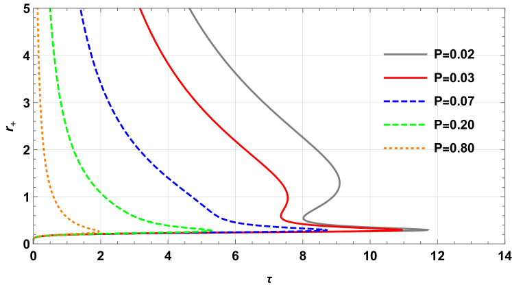
(c) Zero points of $\phi$ for different values of $P$. Here $a=0.1$ and $Q=0.36$

Figure 3: Zero points of $\phi$ in $r_{+}$ vs $\tau$ plane with different parameter variations for EHAdS black hole in canonical ensemble (positive $a$).

Now, we choose a parameter combination $(a,P,Q)=(0.1,0.005,0.36)$ such that

$$\mathcal{A}(z)=0.00167962\tau+0.502655\tau z^{8}+4\tau z^{6}-0.5184\tau z^{4}-16\pi z^{7}.$$ (22)

The plot of $\mathcal{A}(z)$ is shown in Figure 4.

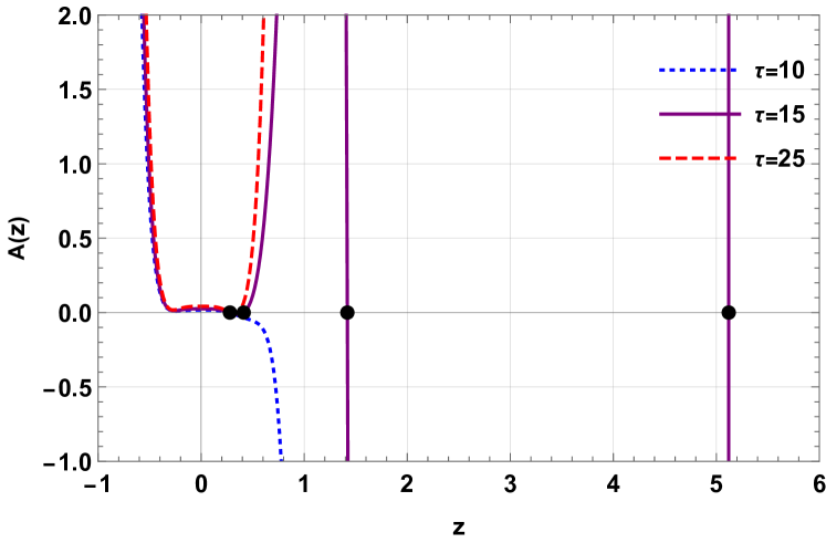
(a) All four roots of $\mathcal{A}(z)$ for $\tau=15$

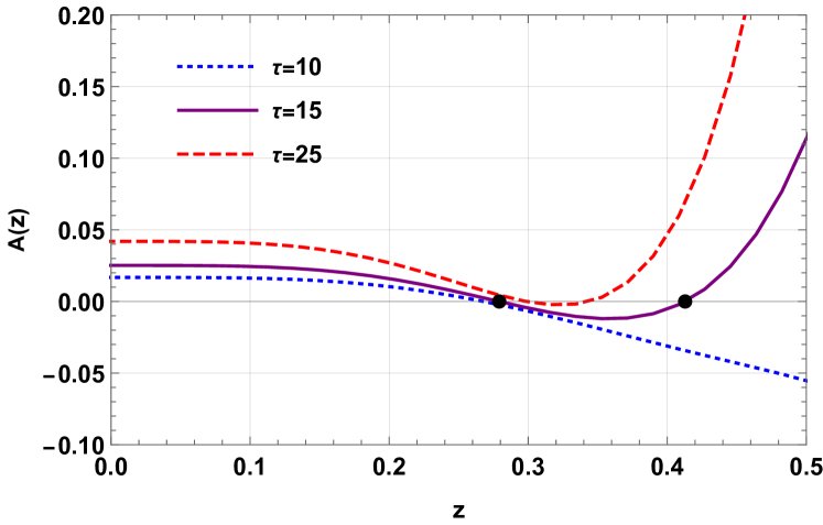
(b) Enlarged view of the two smaller positive roots of $\mathcal{A}(z)$ for $\tau=15$

Figure 4: Plot of the polynomial function $\mathcal{A}(z)$ for $\tau=10,~{}15,\text{and}~{}25$. The black dots represents the roots for $\tau=15$.

Using (22) we can calculate the roots for fixed $\tau$. For $\tau=15$ the roots are shown in Figure 4 as black dots which are are $z_{1}=0.279175,~{}z_{2}=0.412857,~{}z_{3}=1.41885,~{}\text{and}~{}z_{4}=5.12015$. Now using (18) and following the Residue theorem, for each positive real roots, we calculate the winding numbers

$$w_{1}=-1,~{}w_{2}=+1,~{}w_{3}=-1,~{}\text{and}~{}w_{4}=+1.$$ (23)

Clearly, here the topological number is $W=w_{1}+w_{2}+w_{3}+w_{4}=-1+1-1+1=0$. To understand the impact of different parameters in the winding numbers and the topological number, we perform our study for a variety of parameter values. The results are summarized in the Table 2.

EHAdS black hole
Parameters			$\tau$	Winding number	Topological number
P	Q	a
0.005	0.36	0.1	10	$w_{1}=-1$ $w_{2}=+1$	$W=0$
			15	$w_{1}=-1$ $w_{2}=+1$ $w_{3}=-1$ $w_{4}=+1$	$W=0$
			25	$w_{1}=-1$ $w_{2}=+1$	$W=0$
0.005	0.36	0.6	10	$w_{1}=-1$ $w_{2}=+1$	$W=0$
			15	$w_{1}=-1$ $w_{2}=+1$	$W=0$
0.005	0.1	0.1	5	$w_{1}=-1$ $w_{2}=+1$	$W=0$
			10	$w_{1}=-1$ $w_{2}=+1$	$W=0$
			15	$w_{1}=-1$ $w_{2}=+1$	$W=0$
0.005	0.9	0.1	5	$w_{1}=-1$ $w_{2}=+1$	$W=0$
			10	$w_{1}=-1$ $w_{2}=+1$	$W=0$
			15	$w_{1}=-1$ $w_{2}=+1$	$W=0$
			20	$w_{1}=-1$ $w_{2}=+1$	$W=0$
0.2	0.36	0.1	1	$w_{1}=-1$ $w_{2}=+1$	$W=0$
			3	$w_{1}=-1$ $w_{2}=+1$	$W=0$
			5	$w_{1}=-1$ $w_{2}=+1$	$W=0$

Table 2: Winding numbers and Topological numbers for EHAdS black hole in canonical ensemble for positive $a$

III Higher-order QED corrected Euler-Heisenberg-AdS black hole in canonical ensemble

In this section we extend our work to the higher-order QED corrected Euler-Heisenberg-AdS black hole [69, 70]. We study the system by treating it as thermodynamic topological defects and study its topological properties. The higher-order Euler-Heisenberg-AdS black hole is obtained by the higher order QED correction of the EHAdS black hole. In this higher order correction, the metric potential, mass, temperature are modified as

$$f^{\prime}(r)=f(r)+\frac{\beta a^{2}Q^{2}}{36r^{10}},$$ (24)

$$M^{\prime}=M+\frac{\beta a^{2}Q^{6}}{72r_{+}^{9}},$$ (25)

$$T^{\prime}=T-\frac{\beta a^{2}Q^{6}}{16\pi r_{+}^{11}},$$ (26)

where, $f(r)$, $M$ and $T$ are given in (10), (13) and (14). Here, we have an additional parameter $\beta$ which appears as a consequence of the higher order QED correction. The equations (24), (25), and (26) reduces to its corresponding EHAdS black hole thermodynamic parameters when $\beta\rightarrow 0$. Now, the generalized free energy is given as

$$\mathcal{F}=\frac{a^{2}\beta Q^{6}}{72r_{+}^{9}}+\frac{-3aQ^{4}+160\pi Pr_{+}^{8}+60Q^{2}r_{+}^{4}+60r_{+}^{6}}{120r_{+}^{5}}-\frac{\pi r_{+}^{2}}{\tau}$$ (27)

The vector field $\phi$ is defined by (16) and the zero points $\phi$ are given by

$$\tau=\frac{16\pi r_{+}^{11}}{-a^{2}\beta Q^{6}+aQ^{4}r_{+}^{4}+32\pi Pr_{+}^{12}-4Q^{2}r_{+}^{8}+4r_{+}^{10}}.$$ (28)

Using (4) we define the complex function

$$\mathcal{R}_{HOEH}(z)=\frac{-a^{2}\beta Q^{6}+aQ^{4}z^{4}+32\pi Pz^{12}-4Q^{2}z^{8}+4z^{10}}{-a^{2}\beta Q^{6}\tau+aQ^{4}\tau z^{4}+32\pi P\tau z^{12}-4Q^{2}\tau z^{8}+4\tau z^{10}-16\pi z^{11}}.$$ (29)

Denominator of (29) is considered as a polynomial function

$$\mathcal{A}(z)=-a^{2}\beta Q^{6}\tau+aQ^{4}\tau z^{4}+32\pi P\tau z^{12}-4Q^{2}\tau z^{8}+4\tau z^{10}-16\pi z^{11}.$$ (30)

The roots of $\mathcal{A}(z)$ will give the poles of $\mathcal{R}_{HOEH}(z)$.

III.1 For negative $a$

Here, we study the system with $\beta=0.11$ and for $a<0$. The variation of $\tau(r_{+})$ is shown in Figure 5. From these figure we see that $\tau(r_{+})$ can have either $1$ or $3$ different branches depending on the parameters $P$, $Q$, $a$ and $\beta$.

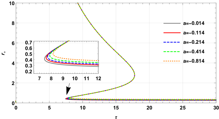
(a) Zero points of $\phi$ for different negative values of $a$. Here $\beta=0.11$, $P=0.005$ and $Q=0.234$.

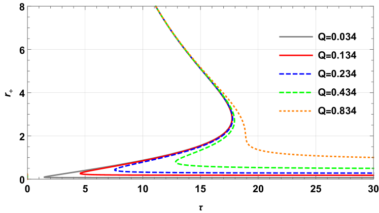
(b) Zero points of $\phi$ for different values of $Q$. Here $\beta=0.11$, $a=-0.114$ and $P=0.005$

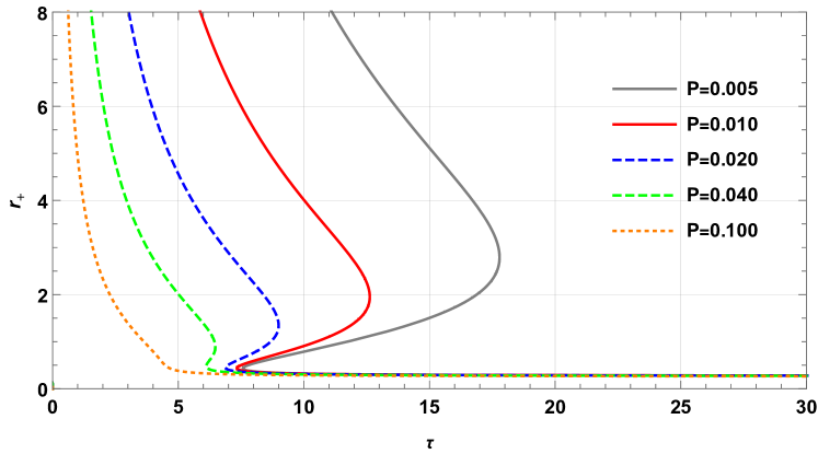
(c) Zero points of $\phi$ for different values of $P$. Here $\beta=0.11$, $a=-0.114$ and $Q=0.36$

Figure 5: $\tau$ vs $r_{+}$ plot with different parameter variations for higher-order QED corrected EHAdS black hole in canonical ensemble (negative $a$).

The polynomial function is calculated from (30) and for $(P,Q,a,\beta)=(0.005,0.234,-0.114,0.11)$ it is given as

$$\mathcal{A}(z)=-2.346915927219771\times 10^{-7}\tau+0.502655\tau z^{12}+4\tau z^{10}-0.219024\tau z^{8}-0.000341797\tau z^{4}-16\pi z^{11}$$ (31)

The roots for different values of $\tau$ is shown in Figure 6. We choose $\tau=15$ and find three real positive roots as $z_{1}=0.296051$, $z_{2}=1.50412$ and $z_{3}=5.11379$. These roots are shown in Figure 6 as black dots.

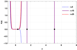
Figure 6: Plot of the polynomial function $\mathcal{A}(z)$ for $\tau=5,~{}15,\text{and}~{}25$. The black dots represents the roots for $\tau=15$.

Now using the residue we calculate their corresponding winding numbers which are $w_{1}=+1$, $w_{2}=-1$, and $w_{3}=+1$. The topological number is hence $W=+1-1+1=+1$. From 5(a) we see that the winding numbers are on the different branches of $\tau(r_{+})$ curve and $w_{1}=w_{3}=+1$ corresponds to the stable black hole region whereas the $w_{2}=-1$ corresponds to the unstable black hole region. We have calculated the winding numbers for different values of the parameters and the results are shown in the Table 3.

Higher order EHAdS black hole ($\beta=0.11$)
Parameters			$\tau$	Winding number	Topological number
P	Q	a
0.005	0.234	-0.114	5	$w_{1}=+1$	$W=+1$
			15	$w_{1}=+1$ $w_{2}=-1$ $w_{3}=+1$	$W=+1$
			20	$w_{1}=+1$	$W=+1$
0.005	0.234	-0.414	4	$w_{1}=+1$	$W=+1$
			10	$w_{1}=+1$ $w_{2}=-1$ $w_{3}=+1$	$W=+1$
			20	$w_{1}=+1$	$W=+1$
0.005	0.034	-0.114	1	$w_{1}=+1$	$W=+1$
			10	$w_{1}=+1$ $w_{2}=-1$ $w_{3}=+1$	$W=+1$
			20	$w_{1}=+1$	$W=+1$
0.1	0.234	-0.114	5	$w_{1}=+1$	$W=+1$
			10	$w_{1}=+1$	$W=+1$
			15	$w_{1}=+1$	$W=+1$

Table 3: Winding numbers and Topological numbers for higher order QED corrected EHAdS black hole in canonical ensemble for negative $a$

III.2 For positive $a$

We repeat our calculation of a positive value of EH parameter $a$. The zero points of $\phi$ i.e. the variation of $\tau(r_{+})$ curve for $\beta=0.11$ and different values of $P$, $Q$, and $a$ are shown in Figure 7. In this case, we observe either $3$ or $5$ different branches of $\tau(r_{+})$. For example, the red line in 7(a), which is for $(P,Q,a,\beta)=(0.005,0.234,0.114,0.11)$ shows five different branches of $\tau(r_{+})$ curve. In this parameter combination the polynomial function is given as

$$\mathcal{A}(z)=-2.346915927219771\times 10^{-7}\tau+0.502655\tau z^{12}+4\tau z^{10}-0.219024\tau z^{8}+0.000341797\tau z^{4}-16\pi z^{11}$$ (32)

The roots of $\mathcal{A}(z)$ for different values of $\tau$ is shown in Figure 8. For $\tau=7.2$ we have five real positive roots of $\mathcal{A}(z)$ which are $z_{1}=0.188142$, $z_{2}=0.233831$, $z_{3}=0.340349$, $z_{4}=0.400221$ and $z_{5}=13.2903$. From the residue theorem we find that the corresponding winding numbers are $w_{1}=+1$, $w_{2}=-1$, $w_{3}=+1$, $w_{4}=-1$, and $w_{5}=+1$. The topological number is hence $W=w_{1}+w_{2}+w_{3}+w_{4}+w_{5}=+1$. The winding numbers $w_{1}=w_{3}=w_{5}=+1$ correspond to the stable black hole region whereas the winding numbers $w_{2}=w_{4}=-1$ correspond to unstable black hole region. The winding numbers as well as the topological numbers with different values of parameters are shown in the Table 4.

(a) Zero points of $\phi$ for different positive values of $a$. Here $\beta=0.11$, $P=0.005$ and $Q=0.234$.

(b) Zero points of $\phi$ for different values of $Q$. Here $\beta=0.11$, $a=0.114$ and $P=0.005$

(c) Zero points of $\phi$ for different values of $P$. Here $\beta=0.11$, $a=0.114$ and $Q=0.36$

Figure 7: $\tau$ vs $r_{+}$ plot with different parameter variations for higher-order QED corrected EHAdS black hole in canonical ensemble (for positive $a$).

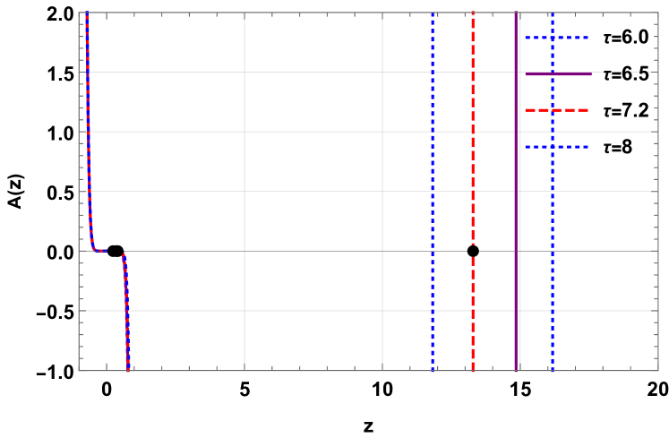
(a) All roots of the polynomial $\mathcal{A}(z)$ for $\tau=7.2$

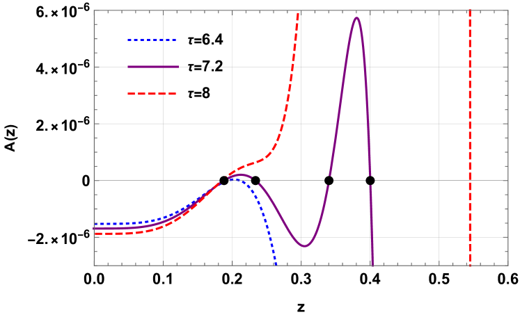
(b) Enlarged view of the two smaller positive roots of $\mathcal{A}(z)$

Figure 8: Plot of the polynomial function $\mathcal{A}(z)$ for $\tau=6,~{}6.5,~{}7.2,\text{and}~{}8$. The black dots represents the roots for $\tau=7.2$.

Higher order EHAdS black hole ($\beta=0.11$)
Parameters			$\tau$	Winding number	Topological number
P	Q	a
0.005	0.234	0.114	6	$w_{1}=+1$	$W=+1$
			6.5	$w_{1}=+1$ $w_{2}=-1$ $w_{3}=+1$	$W=+1$
			7.2	$w_{1}=+1$ $w_{2}=-1$ $w_{3}=+1$ $w_{4}=-1$ $w_{5}=+1$	$W=+1$
			8	$w_{1}=+1$	$W=+1$
0.005	0.234	0.414	4	$w_{1}=+1$	$W=+1$
			10	$w_{1}=+1$ $w_{2}=-1$ $w_{3}=+1$	$W=+1$
			20	$w_{1}=+1$	$W=+1$
0.005	0.034	0.114	2	$w_{1}=+1$ $w_{2}=-1$ $w_{3}=+1$	$W=+1$
			10	$w_{1}=+1$ $w_{2}=-1$ $w_{3}=+1$	$W=+1$
			20	$w_{1}=+1$	$W=+1$
0.1	0.234	0.114	5	$w_{1}=+1$	$W=+1$
			5.2	$w_{1}=+1$ $w_{2}=-1$ $w_{3}=+1$	$W=+1$
			6	$w_{1}=+1$	$W=+1$

Table 4: Winding numbers and Topological numbers for higher order QED corrected EHAdS black hole in canonical ensemble for positive $a$

IV 4D Euler-Heisenberg AdS black hole in grand canonical ensemble

The thermodynamics of black holes may be different in different ensembles. Therefore, we extend our study to the grand canonical ensemble. In this ensemble, the charge $Q$ is written in terms of the electric potential $\phi$ as

$$Q=\frac{-\sqrt[3]{15}\Bigl{\{}r_{+}^{5}\left(\sqrt{3}\sqrt{a^{3}\left(27a\phi_{e}^{2}-40r_{+}^{2}\right)}+9a^{2}\phi_{e}\right)\Bigr{\}}^{2/3}-2\times 15^{2/3}ar_{+}^{4}}{3a\sqrt[3]{r_{+}^{5}\left(\sqrt{3}\sqrt{a^{3}\left(27a\phi_{e}^{2}-40r_{+}^{2}\right)}+9a^{2}\phi_{e}\right)}}$$ (33)

and mass is written as

$$\mathcal{M}= M-Q\phi_{e}$$ (34)

$$= \frac{3\sqrt[6]{3}5^{2/3}r_{+}^{9}\phi_{e}\left(\sqrt{a^{3}\left(27a\phi_{e}^{2}-40r_{+}^{2}\right)}+3\sqrt{3}a^{2}\phi_{e}\right)}{A^{4/3}}-\frac{10\times 5^{2/3}ar_{+}^{11}}{\sqrt[3]{3}A^{4/3}}+\frac{\sqrt[3]{15}\sqrt[3]{A}\phi_{e}}{4a}$$

$$+\frac{r_{+}^{3}(4\pi aP+5)}{3a}+\frac{5\sqrt[3]{5}r_{+}^{7}}{3^{2/3}A^{2/3}}+\frac{r_{+}}{2},$$

where $A=r_{+}^{5}\Bigl{\{}\sqrt{3}\sqrt{a^{3}\left(27a\phi_{e}^{2}-40r_{+}^{2}\right)}+9a^{2}\phi_{e}\Bigr{\}}$ and $M$ is given by (13). The free energy is modified as

$$\mathcal{F}=\mathcal{M}-\frac{S}{\tau}.$$ (35)

The expression for $\tau$ can be calculated by $\partial_{r_{+}}\mathcal{F}=0$. From (4) we calculate the complex function $\mathcal{R}(z)$, the denominator of which is the polynomial function $\mathcal{A}(z)$ (see Equation 40 and Equation 41).

IV.1 For negative $a$

The $\tau(r_{+})$ curve for parameters is shown in Figure 9. Here we see that for different sets of parameters we have two branches of the $\tau$ curve. In 9(a) we see that there is slight variation of the $\tau$ curve with the variation of EH parameter $a$. For higher values of $\phi_{e}$ (such as $\phi_{e}=2,~{}5$) in 9(b) the lower part is not visible but they follow the similar pattern as the other curves. We plot polynomial function $\mathcal{A}(z)$ for a parameter set $(P,\phi_{e},a)=(0.05,0.01,-0.1)$ in Figure 10 and the roots are found to be at $z_{1}=9.91978707$ and $z_{2}=0.0802129245$. Here we choose $\tau=1$ Interestingly, we have found that the roots indicate a second order pole of the complex function $\mathcal{R}(z)$. Using residue method we calculate the winding number. Corresponding to $z_{1}$ and $z_{2}$ the winding numbers are respectively $w_{1}=+1$ and $w_{2}=-1$ yielding topological number $W=w_{1}+w_{2}=0$. We have calculated the winding numbers and topological numbers for different sets of parameters which is represented in the Table 5.

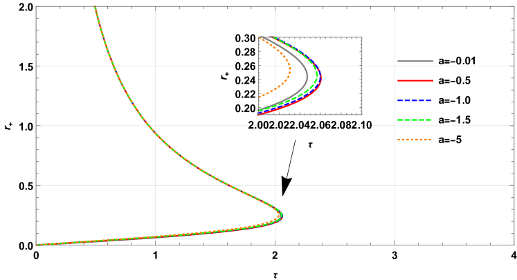
(a) Zero points of $\phi$ for different negative values of $a$. Here $P=0.5$ and $\phi_{e}=0.5$.

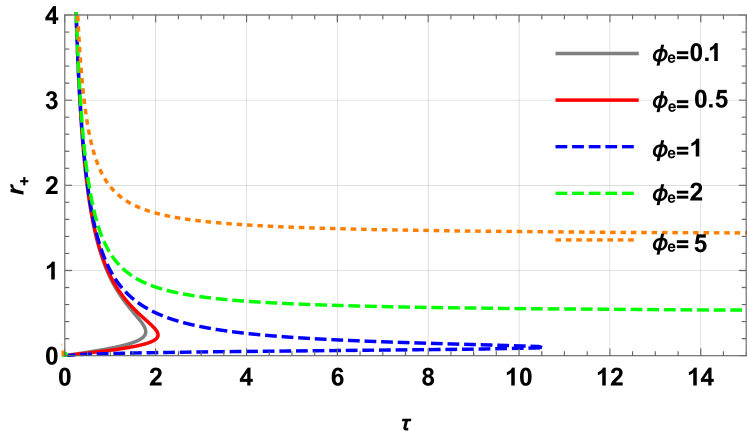
(b) Zero points of $\phi$ for different values of $\phi_{e}$. Here $a=-0.1$ and $P=0.5$

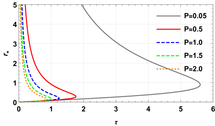
(c) Zero points of $\phi_{e}$ for different values of $P$. Here $a=-0.1$ and $\phi_{e}=0.01$

Figure 9: $\tau$ vs $r_{+}$ plot with different parameter variations for EHAdS black hole in grand canonical ensemble (for negative $a$).

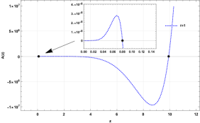
Figure 10: Plot of the polynomial function $\mathcal{A}(z)$ for $\tau=1$. The black dots represent the roots of the polynomial.

EH black hole in grand canonical ensemble
Parameters			$\tau$	Winding number	Topological number
P	$\phi$	a
0.05	0.01	-0.1	1	$w_{1}=+1$ $w_{2}=-1$	$W=0$
0.05	0.01	-1	1	$w_{1}=+1$ $w_{2}=-1$	$W=0$
0.05	0.01	-5	1	$w_{1}=+1$ $w_{2}=-1$	$W=0$
0.5	0.01	-0.1	1	$w_{1}=+1$ $w_{2}=-1$	$W=0$
1.5	0.01	-0.1	0.5	$w_{1}=+1$ $w_{2}=-1$	$W=0$
0.5	0.5	-0.1	1	$w_{1}=+1$ $w_{2}=-1$	$W=0$
0.5	2	-0.1	1	$w_{1}=+1$ $w_{2}=-1$	$W=0$

Table 5: Winding numbers and topological numbers for EHAdS black hole in grand canonical ensemble for negative $a$

IV.2 Positive $a$

Now, we change the sign of the EH parameter $a$ to positive and study the thermodynamic topology. For simplicity, in this case we calculate the winding numbers by drawing contours around the zero points. Using (35) and (16) we calculate the vector field $\phi$ and then, normalized vector field as

$$n=\Bigl{(}\frac{\phi_{r_{+}}}{|\phi|},\frac{\phi_{\Theta}}{|\phi|}\Bigr{)}\quad\quad\text{where,}\quad\phi_{r_{+}}=\frac{\partial\mathcal{F}}{\partial r_{+}},~{}\phi_{\Theta}=-\cot\Theta\csc\Theta.$$ (36)

The zero point can be calculated by setting $\Theta=\pi/2$ in $\phi_{r_{+}}$. The plot of $\tau(r_{+})$ curve is shown in Figure 11 where we observe two black hole branches.

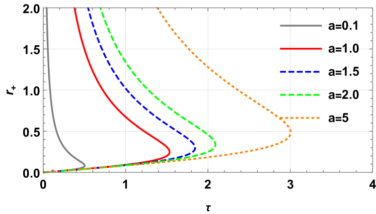
(a) Zero points of $\phi$ for different negative values of $a$. Here $P=0.5$ and $\phi_{e}=0.5$.

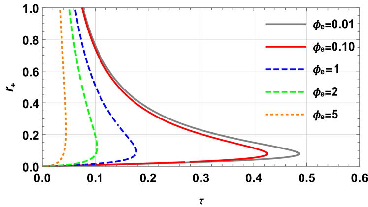
(b) Zero points of $\phi$ for different values of $\phi_{e}$. Here $a=0.1$ and $P=0.5$

(c) Zero points of $\phi_{e}$ for different values of $P$. Here $a=0.1$ and $\phi_{e}=0.01$

Figure 11: $\tau$ vs $r_{+}$ plot with different parameter variations for EHAdS black hole in grand canonical ensemble (for positive $a$).

For $(P,\phi_{e},a)=(0.05,0.01,0.1)$ and $\tau=0.3$ the vector plot of $n$ is shown in Figure 12. The zero points are situated at $(\Theta,r_{+})=(\pi/2,0.24758)~{}\text{and}~{}(\pi/2,0.0267)$. Two contours $C_{1}$ and $C_{2}$ (see Figure 12) are drawn enclosing the zero points which are defined as (2). The zero points $z_{1}=0.24758$ and $z_{2}=0.0267$ respectively corresponds to $w_{1}=+1$ and $w_{2}=-1$ winding number. The topological number is hence $W=+1-1=0$. The winding numbers and the corresponding topological number for various set of parameters are shown in Table 6.

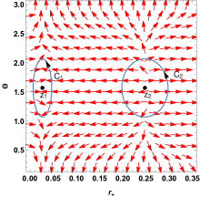
Figure 12: Vector plot of $n$. The black dots represent the zero points.

EH black hole
Parameters			$\tau$	Winding number	Topological number
P	$\phi$	a
0.05	0.01	0.1	0.3	$w_{1}=+1$ $w_{2}=-1$	$W=0$
0.05	0.01	1	1	$w_{1}=+1$ $w_{2}=-1$	$W=0$
0.05	0.01	2	1	$w_{1}=+1$ $w_{2}=-1$	$W=0$
0.5	0.01	0.1	0.3	$w_{1}=+1$ $w_{2}=-1$	$W=0$
1.5	0.01	0.1	0.3	$w_{1}=+1$ $w_{2}=-1$	$W=0$
0.5	0.1	0.1	0.35	$w_{1}=+1$ $w_{2}=-1$	$W=0$
0.5	2	0.1	0.08	$w_{1}=+1$ $w_{2}=-1$	$W=0$

Table 6: Winding numbers and topological numbers for EHAdS black hole in grand canonical ensemble for positive $a$

V Higher order QED corrected Euler-Heisenberg-AdS black hole in grand canonical ensemble

In grand canonical ensemble the charge $Q$ is decomposed to the electric potential $\phi_{e}$. The electric potential is the conjugate of charge. To calculate $\phi_{e}$ we partially differentiate the mass $M^{\prime}$ (see (25)) with respect to $Q$. This provides us

$$\phi_{e}=\frac{a^{2}\beta Q^{5}}{12r_{+}^{9}}+\frac{120Qr_{+}^{4}-12aQ^{3}}{120r_{+}^{5}}.$$ (37)

Writing the charge $Q$ in terms of $\phi_{e}$ using (37), new mass can be calculated using

$$\mathcal{M}= M^{\prime}-Q\phi_{e},$$ (38)

where $M^{\prime}$ is given by (25). The free energy is calculated as

$$\mathcal{F}=\mathcal{M}-\frac{S}{\tau}.$$ (39)

In residue method the complex function $\mathcal{R}(z)$ is defined as (4) and the denominator of this function is the polynomial function $\mathcal{A}(z)$ (see Equation 42 and Equation 43). We choose $\beta=0.11$ for our study.

V.1 Negative $a$

From (39) we calculate the $\tau$ curve using $\frac{\partial\mathcal{F}}{\partial r_{+}}=0$. For different set of parameters the $\tau$ vs $r_{+}$ curve is shown in Figure 13. For different combination of parameters we have two different branches of the $\tau(r_{+})$ curve. To calculate the winding numbers we choose a set of parameters $(P,\phi_{e},a,\beta)=(0.5,1,-0.1,0.11)$ and $\tau=5$. The polynomial function $\mathcal{A}(z)$ is shown in Figure 14. The black dots represent the roots of $\mathcal{A}(z)$ which are $z_{1}=0.2178700113$ and $z_{2}=0.057573538$. From residue method the winding numbers corresponding to $z_{1}$ and $z_{2}$ are obtained as $w_{1}=+1$ and $w_{2}=-1$. The topological number is $W=+1-1=0$. For various set of parameters the winding number and the topological number are shown in Table 7.

(a) $\tau$ vs $r_{+}$ plot for different negative values of $a$. Here $P=0.5$ and $\phi_{e}=1$.

(b) $\tau$ vs $r_{+}$ plot for different values of $\phi_{e}$. Here $a=-0.1$ and $P=0.5$

(c) $\tau$ vs $r_{+}$ plot for different values of $P$. Here $a=-0.1$ and $\phi_{e}=0.01$

Figure 13: $\tau$ vs $r_{+}$ plot with different parameter variations for higher order QED corrected EHAdS black hole in grand canonical ensemble (for negative $a$).

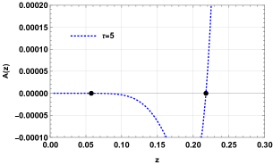
Figure 14: Plot of the polynomial function $\mathcal{A}(z)$ for $\tau=5$. The black dots represent the roots of the polynomial.

Higher order EHAdS black hole in grand canonical ensemble ($\beta=0.11$)
Parameters			$\tau$	Winding number	Topological number
P	$\phi$	a
0.5	1	-0.1	5	$w_{1}=+1$ $w_{2}=-1$	$W=0$
0.5	1	-1	4	$w_{1}=+1$ $w_{2}=-1$	$W=0$
0.5	1	-2	2	$w_{1}=+1$ $w_{2}=-1$	$W=0$
0.5	0.1	-0.1	1	$w_{1}=+1$ $w_{2}=-1$	$W=0$
0.5	0.5	-0.1	2	$w_{1}=+1$ $w_{2}=-1$	$W=0$
0.5	1.5	-0.1	12	$w_{1}=+1$ $w_{2}=-1$	$W=0$
0.5	0.01	-0.1	1	$w_{1}=+1$ $w_{2}=-1$	$W=0$
1	0.01	-0.1	1	$w_{1}=+1$ $w_{2}=-1$	$W=0$
1.5	0.01	-0.1	0.5	$w_{1}=+1$ $w_{2}=-1$	$W=0$

Table 7: Winding numbers and topological numbers for higher order QED corrected EHAdS black hole in grand canonical ensemble for negative $a$

V.2 Positive $a$

For positive EH parameter $a$, the $\tau(r_{+})$ curve is shown in Figure 15 which is observed to have either $2$ or $4$ different branches. In 15(a) we observe four branches of the $\tau(r_{+})$ curve for $(P,\phi_{e},a,\beta)=(0.5,1,0.05,0.11)$. In this parameter combination the polynomial function is shown in Figure 16. For $\tau=4$ we have four roots of $\mathcal{A}(z)$ which are $z_{1}=0.221127$, $z_{2}=0.1724031$, $z_{3}=0.140630$ and $z_{4}=0.017681$. From residue method discussed earlier, the corresponding winding numbers are $w_{1}=+1$, $w_{2}=-1$, $w_{3}=+1$ and $w_{4}=-1$ yielding the topological number to be $W=+1-1+1-1=0$. For the other set of parameters, the $\tau$ curve has two branches with $w_{1}=+1$ and $w_{2}=-1$ winding number. The topological number is hence $W=+1-1=0$. The winding numbers and topological numbers for various set of parameters are shown in Table 8.

(a) $\tau$ vs $r_{+}$ plot for different negative values of $a$. Here $P=0.5$ and $\phi_{e}=1$.

(b) $\tau$ vs $r_{+}$ plot for different values of $\phi_{e}$. Here $a=1$ and $P=0.5$

(c) $\tau$ vs $r_{+}$ plot for different values of $P$. Here $a=1$ and $\phi_{e}=0.1$

Figure 15: $\tau$ vs $r_{+}$ plot with different parameter variations for higher order QED corrected EHAdS black hole in grand canonical ensemble (for positive $a$).

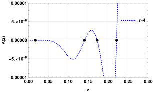
Figure 16: Plot of the polynomial function $\mathcal{A}(z)$ for $\tau=4$. The black dots represent the roots of the polynomial.

Higher order EHAdS black hole in grand canonical ensemble ($\beta=0.11$)
Parameters			$\tau$	Winding number	Topological number
P	$\phi$	a
0.5	1	0.05	4	$w_{1}=+1$ $w_{2}=-1$ $w_{3}=+1$ $w_{4}=-1$	$W=0$
0.5	1	0.5	4	$w_{1}=+1$ $w_{2}=-1$	$W=0$
0.5	1	1	10	$w_{1}=+1$ $w_{2}=-1$	$W=0$
0.5	0.1	2	5	$w_{1}=+1$ $w_{2}=-1$	$W=0$
0.5	0.01	1	1	$w_{1}=+1$ $w_{2}=-1$	$W=0$
0.5	0.1	1	1	$w_{1}=+1$ $w_{2}=-1$	$W=0$
0.5	1.5	1	10	$w_{1}=+1$ $w_{2}=-1$	$W=0$
0.08	0.65	1	5.3	$w_{1}=+1$ $w_{2}=-1$ $w_{3}=+1$ $w_{4}=-1$	$W=0$
0.5	0.1	1	1	$w_{1}=+1$ $w_{2}=-1$	$W=0$
1	0.1	1	1	$w_{1}=+1$ $w_{2}=-1$	$W=0$

Table 8: Winding numbers and topological numbers for higher order QED corrected EHAdS black hole in grand canonical ensemble for positive $a$

VI Conclusion

We have studied the thermodynamic topology of 4D Euler-Heisenberg-AdS black hole in different ensembles without and with the higher order QED correction using generalized off-shell free energy. We calculate the winding number and the topological number for the aforementioned black hole systems for both negative and positive EH parameters $a$ in different ensembles.

For 4D EHAdS black hole in canonical ensemble with negative EH parameter $a$, the $\tau(r_{+})$ curve, which represents the zero points of the vector field $\phi$, is observed to posses either $1$ or $3$ black hole branches depending on the parameters pressure $P$, charge $Q$ and EH parameter $a$. The total topological number is conserved ($W=+1$) regardless of the different values of the thermodynamic parameters. For EHAdS black hole in canonical ensemble with positive EH parameter $a$, the $\tau(r_{+})$ curve is observed to have either $2$ or $4$ black hole branches depending on the thermodynamic parameters. The topological number in this case is $W=0$. Variation of the thermodynamic parameters do not have any impact on the topological number. This implies that the topological class of 4D EHAdS black hole in canonical ensemble changes depending on the signature of EH parameter $a$. We have tabulated our findings in Table 1 and Table 2.

Next, we have studied the thermodynamic topology of the higher-order QED corrected Euler-Heisenberg-AdS black hole. For this black hole system, we set the parameter $\beta=0.11$ and study its thermodynamic topological properties for both the negative and positive values of EH parameter $a$. In canonical ensemble, for the negative $a$, the $\tau(r_{+})$ curve is observed to have either $3$ or $1$ branches depending on the parameters $P$, $Q$ and $a$. The topological number is found to be $W=+1$. Changing the thermodynamic parameters do not have any impact on $W$ i.e., it is conserved. For the positive $a$ case, we have observed either $3$ or $5$ different branches of the $\tau(r_{+})$ curve. The total topological number is also $W=+1$ and it is found to be conserved. Therefore, we conclude that the higher-order QED corrected EHAdS black hole falls under the same topological class regardless of the nature of EH parameter $a$. The results are tabulated in Table 3 and Table 4.

For EHAdS black hole in grand canonical ensemble, with both negative and positive EH parameter $a$, we have observed $2$ different branches of $\tau(r_{+})$ curve, respectively corresponding to positive and negative winding number. The topological number is hence $W=0$. In case of the higher order QED corrected EHAdS black hole, for negative EH parameter $a$ and $\beta=0.11$, we have found $2$ different branches of the $\tau(r_{+})$ curve. On the other hand, for the same, with positive EH parameter $a$ and $\beta=0.11$, we have found either $2$ or $4$ different branches of the $\tau(r_{+})$ curve. The topological number for both the black hole systems in grand canonical ensemble is found to be $W=0$ which is independent of the parameters pressure $P$, electric potential $\phi_{e}$ and EH parameter $a$. This suggests that the EHAdS black hole and the higher order QED corrected EHAdS black hole in grand canonical ensemble belong to the same topological class. The winding numbers and topological numbers for various set of parameters are shown in Table 5, Table 6, Table 7 and Table 8.

An interesting question whether the currently known thermodynamic topological classification will hold good for other black hole solutions in different theories of gravity. We plan to address this question in our future works.

VII Declaration

The preparation of this manuscript is not assisted with any funds.

*

Appendix A The complex functions and polynomial functions

A.1 The Euler-Heisenberg AdS black hole in grand canonical ensemble

The complex function $\mathcal{R}(z)$ is given as

$$\mathcal{R}(z)=\frac{\begin{aligned} &-10Az^{11/3}\left(\sqrt[3]{15}z^{5/3}\phi\sqrt[3]{9\phi a^{2}+A\sqrt{3}}+120z^{3}\right)\sqrt[3]{9\phi a^{2}+A\sqrt{3}}\\ &+486\sqrt[6]{3}a^{4}z\phi^{3}\left(\sqrt[3]{3}z^{5/3}\left(8P\pi z^{2}+1\right)\sqrt[3]{9\phi a^{2}+A\sqrt{3}}+14\times 5^{2/3}z^{3}\phi\right)\\ &-6a^{2}\Bigl{\{}-27Az^{8/3}\phi^{2}\sqrt[3]{9\phi a^{2}+A\sqrt{3}}-216AP\pi z^{14/3}\phi^{2}\sqrt[3]{9\phi a^{2}+A\sqrt{3}}+1200z^{20/3}\phi\sqrt{3}\sqrt[3]{9\phi a^{2}+A\sqrt{3}}\\ &+55\times 3^{5/6}\sqrt[3]{5}z^{16/3}\phi^{2}\left(9\phi a^{2}+A\sqrt{3}\right)^{2/3}-400\sqrt[6]{3}5^{2/3}z^{8}-126\times 15^{2/3}Az^{4}\phi^{3}\Bigr{\}})\\ &+45a^{3}\Bigl{\{}-16\sqrt{3}z^{14/3}\left(8P\pi z^{2}+1\right)\phi\sqrt[3]{9\phi a^{2}+A\sqrt{3}}+108z^{14/3}\phi^{3}\sqrt{3}\sqrt[3]{9\phi a^{2}+A\sqrt{3}}\\ &+9\times 3^{5/6}\sqrt[3]{5}z^{10/3}\phi^{4}\left(9\phi a^{2}+A\sqrt{3}\right)^{2/3}-260\sqrt[6]{3}5^{2/3}z^{6}\phi^{2}\Bigr{\}}\\ &-5a\Bigl{\{}-324Az^{14/3}\phi^{2}\sqrt[3]{9\phi a^{2}+A\sqrt{3}}+8z^{14/3}\Bigl{(}10\times 3^{5/6}\sqrt[3]{5}z^{8/3}\sqrt[3]{9\phi a^{2}+A\sqrt{3}}\\ &+24AP\pi z^{2}+3A\Bigr{)}\sqrt[3]{9\phi a^{2}+A\sqrt{3}}-27\sqrt[3]{15}Az^{10/3}\phi^{3}\left(9\phi a^{2}+A\sqrt{3}\right)^{2/3}+148\times 15^{2/3}Az^{6}\phi\Bigr{\}}\end{aligned}}{\begin{aligned} &-10Az^{11/3}\tau\left(\sqrt[3]{15}z^{5/3}\phi\sqrt[3]{9\phi a^{2}+A\sqrt{3}}+120z^{3}\right)\sqrt[3]{9\phi a^{2}+A\sqrt{3}}\\ &+45a^{3}\Bigl{\{}-16\sqrt{3}z^{14/3}\Big{(}\tau+4\pi z(2Pz\tau-1)\Big{)}\phi\sqrt[3]{9\phi a^{2}+A\sqrt{3}}+108z^{14/3}\tau\phi^{3}\sqrt{3}\sqrt[3]{9\phi a^{2}+A\sqrt{3}}\\ &+9\times 3^{5/6}\sqrt[3]{5}z^{10/3}\tau\phi^{4}\left(9\phi a^{2}+A\sqrt{3}\right)^{2/3}-260\sqrt[6]{3}5^{2/3}z^{6}\tau\phi^{2}\Bigr{\}}\\ &+486\sqrt[6]{3}a^{4}z\phi^{3}\Bigl{\{}4\sqrt[3]{3}\pi z^{8/3}(2Pz\tau-1)\sqrt[3]{9\phi a^{2}+A\sqrt{3}}+\tau\left(\sqrt[3]{3}z^{5/3}\sqrt[3]{9\phi a^{2}+A\sqrt{3}}+14\times 5^{2/3}z^{3}\phi\right)\Bigr{\}}\\ &+6a^{2}\Bigl{[}-1200\sqrt{3}z^{20/3}\tau\phi\sqrt[3]{9\phi a^{2}+A\sqrt{3}}+z^{8/3}\phi^{2}\Bigl{\{}-553^{5/6}\sqrt[3]{5}z^{8/3}\tau\sqrt[3]{9\phi a^{2}+A\sqrt{3}}\\ &+27A\tau+108A\pi z(2Pz\tau-1)\Bigr{\}}\sqrt[3]{9\phi a^{2}+A\sqrt{3}}+126\times 15^{2/3}Az^{4}\tau\phi^{3}+400\sqrt[6]{3}5^{2/3}z^{8}\tau\Bigr{]}\\ &-5a\Bigl{[}96A\pi z^{17/3}(2Pz\tau-1)\sqrt[3]{9\phi a^{2}+A\sqrt{3}}+\tau\Bigl{\{}24Az^{14/3}\sqrt[3]{9\phi a^{2}+A\sqrt{3}}-324Az^{14/3}\phi^{2}\sqrt[3]{9\phi a^{2}+A\sqrt{3}}\\ &+80\times 3^{5/6}\sqrt[3]{5}z^{22/3}\left(9\phi a^{2}+A\sqrt{3}\right)^{2/3}-27\sqrt[3]{15}Az^{10/3}\phi^{3}\left(9\phi a^{2}+A\sqrt{3}\right)^{2/3}+148\times 15^{2/3}Az^{6}\phi\Bigr{\}}\Bigr{]}\end{aligned}}$$ (40)

and the polynomial function $\mathcal{A}(z)$ is given as

$$\mathcal{A}(z)= -10Az^{11/3}\tau\left(\sqrt[3]{15}z^{5/3}\phi\sqrt[3]{9\phi a^{2}+A\sqrt{3}}+120z^{3}\right)\sqrt[3]{9\phi a^{2}+A\sqrt{3}}$$ (41)

$$+45a^{3}\Bigl{\{}-16\sqrt{3}z^{14/3}\Big{(}\tau+4\pi z(2Pz\tau-1)\Big{)}\phi\sqrt[3]{9\phi a^{2}+A\sqrt{3}}+108z^{14/3}\tau\phi^{3}\sqrt{3}\sqrt[3]{9\phi a^{2}+A\sqrt{3}}$$

$$+9\times 3^{5/6}\sqrt[3]{5}z^{10/3}\tau\phi^{4}\left(9\phi a^{2}+A\sqrt{3}\right)^{2/3}-260\sqrt[6]{3}5^{2/3}z^{6}\tau\phi^{2}\Bigr{\}}$$

$$+486\sqrt[6]{3}a^{4}z\phi^{3}\Bigl{\{}4\sqrt[3]{3}\pi z^{8/3}(2Pz\tau-1)\sqrt[3]{9\phi a^{2}+A\sqrt{3}}+\tau\left(\sqrt[3]{3}z^{5/3}\sqrt[3]{9\phi a^{2}+A\sqrt{3}}+14\times 5^{2/3}z^{3}\phi\right)\Bigr{\}}$$

$$+6a^{2}\Bigl{[}-1200\sqrt{3}z^{20/3}\tau\phi\sqrt[3]{9\phi a^{2}+A\sqrt{3}}+z^{8/3}\phi^{2}\Bigl{\{}-553^{5/6}\sqrt[3]{5}z^{8/3}\tau\sqrt[3]{9\phi a^{2}+A\sqrt{3}}$$

$$+27A\tau+108A\pi z(2Pz\tau-1)\Bigr{\}}\sqrt[3]{9\phi a^{2}+A\sqrt{3}}+126\ 15^{2/3}Az^{4}\tau\phi^{3}+400\sqrt[6]{3}5^{2/3}z^{8}\tau\Bigr{]}$$

$$-5a\Bigl{[}96A\pi z^{17/3}(2Pz\tau-1)\sqrt[3]{9\phi a^{2}+A\sqrt{3}}+\tau\Bigl{\{}24Az^{14/3}\sqrt[3]{9\phi a^{2}+A\sqrt{3}}-324Az^{14/3}\phi^{2}\sqrt[3]{9\phi a^{2}+A\sqrt{3}}$$

$$+80\times 3^{5/6}\sqrt[3]{5}z^{22/3}\left(9\phi a^{2}+A\sqrt{3}\right)^{2/3}-27\sqrt[3]{15}Az^{10/3}\phi^{3}\left(9\phi a^{2}+A\sqrt{3}\right)^{2/3}+148\times 15^{2/3}Az^{6}\phi\Bigr{\}}\Bigr{]}$$

where, $A=\sqrt{a^{3}\left(27a\phi^{2}-40z^{2}\right)}$.

A.2 The higher order Euler-Heisenberg AdS black hole in grand canonical ensemble

The complex function $\mathcal{R}(z)$ (as standard mathematica output) is given as

$$\mathcal{R}(z)=\frac{\begin{aligned} &a\Bigl{\{}625a\beta^{2}+2z^{2}\left(2500\pi a\beta^{2}P+450\beta-9\right)\Bigr{\}}\text{Root}\left[-\frac{5\text{$\#$1}^{5}a^{2}\beta}{z^{9}}+\frac{6\text{$\#$1}^{3}a}{z^{5}}-\frac{60\text{$\#$1}}{z}+60\phi\&,1\right]^{4}\\ &-30\Bigl{[}2z^{6}\big{\{}20\beta(3\pi aP+10)-3\bigr{\}}+15a\beta z^{4}\Bigr{]}\text{Root}\left[-\frac{5\text{$\#$1}^{5}a^{2}\beta}{z^{9}}+\frac{6\text{$\#$1}^{3}a}{z^{5}}-\frac{60\text{$\#$1}}{z}+60\phi\&,1\right]^{2}\\ &+60(550\beta-3)z^{7}\phi\text{Root}\left[-\frac{5\text{$\#$1}^{5}a^{2}\beta}{z^{9}}+\frac{6\text{$\#$1}^{3}a}{z^{5}}-\frac{60\text{$\#$1}}{z}+60\phi\&,1\right]\\ &-1275a\beta z^{3}\phi\text{Root}\left[-\frac{5\text{$\#$1}^{5}a^{2}\beta}{z^{9}}+\frac{6\text{$\#$1}^{3}a}{z^{5}}-\frac{60\text{$\#$1}}{z}+60\phi\&,1\right]^{3}+1500\beta z^{8}\left(8\pi Pz^{2}-15\phi^{2}+1\right)\end{aligned}}{\begin{aligned} &a\Bigl{[}625a\beta^{2}\bigl{\{}4\pi z(2P\tau z-1)+\tau\bigr{\}}+18(50\beta-1)\tau z^{2}\Bigr{]}\text{Root}\left[-\frac{5\text{$\#$1}^{5}a^{2}\beta}{z^{9}}+\frac{6\text{$\#$1}^{3}a}{z^{5}}-\frac{60\text{$\#$1}}{z}+60\phi\&,1\right]^{4}\\ &-30\Bigl{[}15a\beta z^{4}\bigl{\{}4\pi z(2P\tau z-1)+\tau\bigr{\}}+2(200\beta-3)\tau z^{6}\Bigr{]}\text{Root}\left[-\frac{5\text{$\#$1}^{5}a^{2}\beta}{z^{9}}+\frac{6\text{$\#$1}^{3}a}{z^{5}}-\frac{60\text{$\#$1}}{z}+60\phi\&,1\right]^{2}\\ &+60(550\beta-3)\tau z^{7}\phi\text{Root}\left[-\frac{5\text{$\#$1}^{5}a^{2}\beta}{z^{9}}+\frac{6\text{$\#$1}^{3}a}{z^{5}}-\frac{60\text{$\#$1}}{z}+60\phi\&,1\right]\\ &-1275a\beta\tau z^{3}\phi\text{Root}\left[-\frac{5\text{$\#$1}^{5}a^{2}\beta}{z^{9}}+\frac{6\text{$\#$1}^{3}a}{z^{5}}-\frac{60\text{$\#$1}}{z}+60\phi\&,1\right]^{3}+1500\beta z^{8}\bigl{\{}4\pi z(2P\tau z-1)-15\tau\phi^{2}+\tau\bigr{\}}\end{aligned}}$$ (42)

and the polynomial function $\mathcal{A}(z)$ (as standard mathematica output) is given as

$$\mathcal{A}(z)= a\Bigl{[}625a\beta^{2}\bigl{\{}4\pi z(2P\tau z-1)+\tau\bigr{\}}+18(50\beta-1)\tau z^{2}\Bigr{]}\text{Root}\left[-\frac{5\text{$\#$1}^{5}a^{2}\beta}{z^{9}}+\frac{6\text{$\#$1}^{3}a}{z^{5}}-\frac{60\text{$\#$1}}{z}+60\phi\&,1\right]^{4}$$ (43)

$$-30\Bigl{[}15a\beta z^{4}\bigl{\{}4\pi z(2P\tau z-1)+\tau\bigr{\}}+2(200\beta-3)\tau z^{6}\Bigr{]}\text{Root}\left[-\frac{5\text{$\#$1}^{5}a^{2}\beta}{z^{9}}+\frac{6\text{$\#$1}^{3}a}{z^{5}}-\frac{60\text{$\#$1}}{z}+60\phi\&,1\right]^{2}$$

$$+60(550\beta-3)\tau z^{7}\phi\text{Root}\left[-\frac{5\text{$\#$1}^{5}a^{2}\beta}{z^{9}}+\frac{6\text{$\#$1}^{3}a}{z^{5}}-\frac{60\text{$\#$1}}{z}+60\phi\&,1\right]$$

$$-1275a\beta\tau z^{3}\phi\text{Root}\left[-\frac{5\text{$\#$1}^{5}a^{2}\beta}{z^{9}}+\frac{6\text{$\#$1}^{3}a}{z^{5}}-\frac{60\text{$\#$1}}{z}+60\phi\&,1\right]^{3}+1500\beta z^{8}\bigl{\{}4\pi z(2P\tau z-1)-15\tau\phi^{2}+\tau\bigr{\}}$$

References

- [1] S. W. Hawking, Black hole explosions? Nature 248, 30 (1974). 89, 92, 96.
- [2] J. D. Bekenstein, Black holes and entropy, Phys. Rev. D 7, 2333 (1973).
- [3] S.W. Hawking, Particle Creation by Black Holes, Commun. Math. Phys., 43:199–220, 1975. [Erratum: Commun.Math.Phys. 46, 206 (1976)].
- [4] J.D. Bekenstein, Black holes and the second law, Lett. Nuovo Cim., 4:737–740, 1972.
- [5] Jacob D. Bekenstein, Black holes and entropy, Phys. Rev. D, 7:2333–2346, 1973.
- [6] James M. Bardeen, B. Carter, and S.W. Hawking, The Four laws of black hole mechanics, Commun. Math. Phys., 31:161–170, 1973.
- [7] Robert M. Wald, Entropy and black-hole thermodynamics, Phys. Rev. D, 20:1271–1282, Sep 1979.
- [8] Jacob D Bekenstein. Black-hole thermodynamics, Physics Today, 33(1):24–31, 1980.
- [9] R. M. Wald, The thermodynamics of black holes, Living Rev. Rel. 4, 6 (2001) doi:10.12942/lrr-2001-6 [arXiv:gr-qc/9912119 [gr-qc]].
- [10] S.Carlip, Black Hole Thermodynamics, Int. J. Mod. Phys. D 23, 1430023 (2014) doi:10.1142/S0218271814300237 [arXiv:1410.1486 [gr-qc]].
- [11] A.C.Wall, A Survey of Black Hole Thermodynamics, [arXiv:1804.10610 [gr-qc]].
- [12] P.Candelas and D.W.Sciama, Irreversible Thermodynamics of Black Holes, Phys. Rev. Lett. 38, 1372-1375 (1977) doi:10.1103/PhysRevLett.38.1372
- [13] A. Chamblin, R. Emparan, C. V. Johnson and R. C. Myers, Holography, thermodynamics and fluctuations of charged AdS black holes, Phys. Rev. D 60, 104026 (1999) doi:10.1103/PhysRevD.60.104026 [arXiv:hep-th/9904197 [hep-th]].
- [14] S. W. Hawking and D. N. Page, Thermodynamics of Black Holes in anti-De Sitter Space, Commun. Math. Phys. 87, 577 (1983) doi:10.1007/BF01208266
- [15] A. Chamblin, R. Emparan, C. V. Johnson and R. C. Myers, Charged AdS black holes and catastrophicmholography, Phys. Rev. D 60, 064018 (1999) doi:10.1103/PhysRevD.60.064018 [arXiv:hep-th/9902170 [hep-th]].
- [16] D. Kastor, S. Ray and J. Traschen, Enthalpy and the Mechanics of AdS Black Holes, Class. Quant. Grav. 26, 195011 (2009) doi:10.1088/0264-9381/26/19/195011 [arXiv:0904.2765 [hep-th]].
- [17] S. Gunasekaran, R. B. Mann and D. Kubiznak, Extended phase space thermodynamics for charged and rotating black holes and Born-Infeld vacuum polarization, JHEP 11, 110 (2012) doi:10.1007/JHEP11(2012)110 [arXiv:1208.6251 [hep-th]].
- [18] B. P. Dolan, Where Is the PdV in the First Law of Black Hole Thermodynamics?, doi:10.5772/52455 [arXiv:1209.1272 [gr-qc]].
- [19] D. Chen, G. qingyu and J. Tao, The modified first laws of thermodynamics of anti-de Sitter and de Sitter space–times, Nucl. Phys. B 918, 115-128 (2017) doi:10.1016/j.nuclphysb.2017.02.020 [arXiv:1607.05445 [hep-th]].
- [20] D. Kubiznak and R. B. Mann, P-V criticality of charged AdS black holes, JHEP 07, 033 (2012) doi:10.1007/JHEP07(2012)033 [arXiv:1205.0559 [hep-th]].
- [21] N. Altamirano, D. Kubiznak and R. B. Mann, Reentrant phase transitions in rotating anti–de Sitter black holes, Phys. Rev. D 88, no.10, 101502 (2013) doi:10.1103/PhysRevD.88.101502 [arXiv:1306.5756 [hep-th]].
- [22] N. Altamirano, D. Kubizňák, R. B. Mann and Z. Sherkatghanad, Kerr-AdS analogue of triple point and solid/liquid/gas phase transition, Class. Quant. Grav. 31, 042001 (2014) doi:10.1088/0264-9381/31/4/042001 [arXiv:1308.2672 [hep-th]].
- [23] S. W. Wei and Y. X. Liu, Triple points and phase diagrams in the extended phase space of charged Gauss-Bonnet black holes in AdS space, Phys. Rev. D 90, no.4, 044057 (2014) doi:10.1103/PhysRevD.90.044057 [arXiv:1402.2837 [hep-th]].
- [24] A. M. Frassino, D. Kubiznak, R. B. Mann and F. Simovic, Multiple Reentrant Phase Transitions and Triple Points in Lovelock Thermodynamics, JHEP 09, 080 (2014) doi:10.1007/JHEP09(2014)080 [arXiv:1406.7015 [hep-th]].
- [25] R. G. Cai, L. M. Cao, L. Li and R. Q. Yang, P-V criticality in the extended phase space of Gauss-Bonnet black holes in AdS space, JHEP 09, 005 (2013) doi:10.1007/JHEP09(2013)005 [arXiv:1306.6233 [gr-qc]].
- [26] H. Xu, W. Xu and L. Zhao, Extended phase space thermodynamics for third order Lovelock black holes in diverse dimensions, Eur. Phys. J. C 74, no.9, 3074 (2014) doi:10.1140/epjc/s10052-014-3074-1 [arXiv:1405.4143 [gr-qc]].
- [27] B. P. Dolan, A. Kostouki, D. Kubiznak and R. B. Mann, Isolated critical point from Lovelock gravity, Class. Quant. Grav. 31, no.24, 242001 (2014) doi:10.1088/0264-9381/31/24/242001 [arXiv:1407.4783 [hep-th]].
- [28] R. A. Hennigar, W. G. Brenna and R. B. Mann, P-v criticality in quasitopological gravity, JHEP 07, 077 (2015) doi:10.1007/JHEP07(2015)077 [arXiv:1505.05517 [hep-th]].
- [29] R. A. Hennigar and R. B. Mann, Reentrant phase transitions and van der Waals behaviour for hairy black holes, Entropy 17, no.12, 8056-8072 (2015) doi:10.3390/e17127862 [arXiv:1509.06798 [hep-th]].
- [30] R. A. Hennigar, R. B. Mann and E. Tjoa, Superfluid Black Holes, Phys. Rev. Lett. 118, no.2, 021301 (2017) doi:10.1103/PhysRevLett.118.021301 [arXiv:1609.02564 [hep-th]].
- [31] D. C. Zou, R. Yue and M. Zhang, Reentrant phase transitions of higher-dimensional AdS black holes in dRGT massive gravity, Eur. Phys. J. C 77, no.4, 256 (2017) doi:10.1140/epjc/s10052-017-4822-9 [arXiv:1612.08056 [gr-qc]].
- [32] N. J. Gogoi and P. Phukon, Thermodynamic geometry of 5D -charged black holes in extended thermodynamic space, Phys. Rev. D 103, no.12, 126008 (2021) doi:10.1103/physrevd.103.126008
- [33] N. J. Gogoi, G. K. Mahanta and P. Phukon, Geodesics in geometrothermodynamics (GTD) type II geometry of 4D asymptotically anti-de-Sitter black holes,Eur. Phys. J. Plus 138, no.4, 345 (2023) doi:10.1140/epjp/s13360-023-03938-x
- [34] S. W. Wei and Y. X. Liu, Topology of black hole thermodynamics, Phys. Rev. D 105, no.10, 104003 (2022) doi:10.1103/PhysRevD.105.104003 [arXiv:2112.01706 [gr-qc]].
- [35] Y. S. Duan, The structure of the topological current, SLAC-PUB-3301, (1984).
- [36] S. W. Wei, Y. X. Liu and R. B. Mann, Phys. Rev. Lett. 129, no.19, 191101 (2022) doi:10.1103/PhysRevLett.129.191101 [arXiv:2208.01932 [gr-qc]].
- [37] D. Wu, Topological classes of rotating black holes, Phys. Rev. D 107, no.2, 024024 (2023) doi:10.1103/PhysRevD.107.024024 [arXiv:2211.15151 [gr-qc]].
- [38] C. Liu and J. Wang, Topological natures of the Gauss-Bonnet black hole in AdS space, Phys. Rev. D 107, no.6, 064023 (2023) doi:10.1103/PhysRevD.107.064023 [arXiv:2211.05524 [gr-qc]].
- [39] Z. Y. Fan, Topological interpretation for phase transitions of black holes, Phys. Rev. D 107, no.4, 044026 (2023) doi:10.1103/PhysRevD.107.044026 [arXiv:2211.12957 [gr-qc]].
- [40] N. J. Gogoi and P. Phukon, Topology of thermodynamics in R-charged black holes, Phys. Rev. D 107, no.10, 106009 (2023) doi:10.1103/PhysRevD.107.106009
- [41] N. J. Gogoi and P. Phukon, Thermodynamic topology of 4D dyonic AdS black holes in different ensembles, Phys. Rev. D 108, no.6, 066016 (2023) doi:10.1103/PhysRevD.108.066016 [arXiv:2304.05695 [hep-th]].
- [42] X. Ye and S. W. Wei, Topological study of equatorial timelike circular orbit for spherically symmetric (hairy) black holes, [arXiv:2301.04786 [gr-qc]].
- [43] M. Zhang and J. Jiang, Bulk-boundary thermodynamic equivalence: a topology viewpoint, [arXiv:2303.17515 [hep-th]].
- [44] Y. Du and X. Zhang, Topological classes of black holes in de-Sitter spacetime, [arXiv:2303.13105 [gr-qc]].
- [45] T. Sharqui, Topological Nature of Black Hole Solutions in Massive Gravity, [arXiv:2304.02889 [gr-qc]].
- [46] Y. Du and X. Zhang, Topological classes of BTZ black holes, [arXiv:2302.11189 [gr-qc]].
- [47] D. Wu and S. Q. Wu, Topological classes of thermodynamics of rotating AdS black holes, Phys. Rev. D 107, no.8, 084002 (2023) doi:10.1103/PhysRevD.107.084002 [arXiv:2301.03002 [hep-th]].
- [48] D. Wu, Classifying topology of consistent thermodynamics of the four-dimensional neutral Lorentzian NUT-charged spacetimes, [arXiv:2302.01100 [gr-qc]].
- [49] M. S. Ali, H. El Moumni, J. Khalloufi and K. Masmar, Topology of Born-Infeld-AdS Black Hole Phase Transition, [arXiv:2306.11212 [hep-th]].
- [50] J. Sadeghi, M. A. S. Afshar, S. Noori Gashti and M. R. Alipour, Thermodynamic topology of black holes from bulk-boundary, extended, and restricted phase space perspectives, Annals Phys. 460, 169569 (2024) doi:10.1016/j.aop.2023.169569 [arXiv:2312.04325 [hep-th]].
- [51] M. A. Saleem and A. Taani, The chaotic behavior of black holes: Investigating a topological retraction in anti-de Sitter spaces, New Astron. 107, 102149 (2024) doi:10.1016/j.newast.2023.102149
- [52] M. U. Shahzad, A. Mehmood, S. Sharif and A. Övgün, Criticality and topological classes of neutral Gauss–Bonnet AdS black holes in 5D, Annals Phys. 458, no.3, 169486 (2023) doi:10.1016/j.aop.2023.169486
- [53] Z. Q. Chen and S. W. Wei, Thermodynamics, Ruppeiner geometry, and topology of Born-Infeld black hole in asymptotic flat spacetime, Nucl. Phys. B 996, 116369 (2023) doi:10.1016/j.nuclphysb.2023.116369
- [54] N. C. Bai, L. Li and J. Tao, Topology of black hole thermodynamics in Lovelock gravity, Phys. Rev. D 107, no.6, 064015 (2023) doi:10.1103/PhysRevD.107.064015 [arXiv:2208.10177 [gr-qc]].
- [55] P. K. Yerra and C. Bhamidipati, Topology of black hole thermodynamics in Gauss-Bonnet gravity, Phys. Rev. D 105, no.10, 104053 (2022) doi:10.1103/PhysRevD.105.104053 [arXiv:2202.10288 [gr-qc]].
- [56] B. Hazarika and P. Phukon, Thermodynamic Topology of Horava Lifshitz Black Hole in Two Ensembles, [arXiv:2312.06324 [hep-th]].
- [57] A. Mehmood and M. U. Shahzad, Thermodynamic Topological Classifications of Well-Known Black Holes, [arXiv:2310.09907 [hep-th]].
- [58] C. W. Tong, B. H. Wang and J. R. Sun, Topology of black hole thermodynamics via Rényi statistics, [arXiv:2310.09602 [gr-qc]].
- [59] Y. S. Wang, Z. M. Xu and B. Wu, Thermodynamic phase transition and winding number for the third-order Lovelock black hole, [arXiv:2307.01569 [gr-qc]].
- [60] J. Sadeghi, M. R. Alipour, S. Noori Gashti and M. A. S. Afshar, Bulk-boundary and RPS Thermodynamics from Topology perspective, [arXiv:2306.16117 [gr-qc]].
- [61] D. Wu, Consistent thermodynamics and topological classes for the four-dimensional Lorentzian charged Taub-NUT spacetimes, Eur. Phys. J. C 83, no.7, 589 (2023) doi:10.1140/epjc/s10052-023-11782-7 [arXiv:2306.02324 [gr-qc]].
- [62] D. Wu, Topological classes of thermodynamics of the four-dimensional static accelerating black holes, Phys. Rev. D 108, no.8, 084041 (2023) doi:10.1103/PhysRevD.108.084041 [arXiv:2307.02030 [hep-th]].
- [63] C. Fang, J. Jiang and M. Zhang, Revisiting thermodynamic topologies of black holes, JHEP 01, 102 (2023) doi:10.1007/JHEP01(2023)102 [arXiv:2211.15534 [gr-qc]].
- [64] T. N. Hung and C. H. Nam, Topology in thermodynamics of regular black strings with Kaluza-Klein reduction, [arXiv:2305.15910 [gr-qc]].
- [65] R. Li, C. Liu, K. Zhang and J. Wang, Topology of the landscape and dominant kinetic path for the thermodynamic phase transition of the charged Gauss-Bonnet AdS black holes, [arXiv:2302.06201 [gr-qc]].
- [66] I. H. Salazar, A. Garcia and J. Plebanski, Duality Rotations and Type Solutions to Einstein Equations With Nonlinear Electromagnetic Sources, J. Math. Phys. 28, 2171-2181 (1987) doi:10.1063/1.527430
- [67] D. Magos and N. Bretón, Thermodynamics of the Euler-Heisenberg-AdS black hole, Phys. Rev. D 102, no.8, 084011 (2020) doi:10.1103/PhysRevD.102.084011 [arXiv:2009.05904 [gr-qc]].
- [68] H. Dai, Z. Zhao and S. Zhang, Thermodynamic phase transition of Euler-Heisenberg-AdS black hole on free energy landscape, Nucl. Phys. B 991, 116219 (2023) doi:10.1016/j.nuclphysb.2023.116219 [arXiv:2202.14007 [gr-qc]].
- [69] X. Ye, Z. Q. Chen, M. D. Li and S. W. Wei, QED effects on phase transition and Ruppeiner geometry of Euler-Heisenberg-AdS black holes*, Chin. Phys. C 46, no.11, 115102 (2022) doi:10.1088/1674-1137/ac814d [arXiv:2202.09053 [gr-qc]].
- [70] G. R. Li, S. Guo and E. W. Liang, High-order QED correction impacts on phase transition of the Euler-Heisenberg AdS black hole, Phys. Rev. D 106, no.6, 064011 (2022) doi:10.1103/PhysRevD.106.064011 [arXiv:2111.10812 [hep-th]].
- [71] M. R. Alipour, M. A. S. Afshar, S. Noori Gashti and J. Sadeghi, Topological classification and black hole thermodynamics, [arXiv:2305.05595 [gr-qc]].