Relativistic heat conduction in the large-flux regime

Abstract

We propose a general procedure for evaluating, directly from microphysics, the constitutive relations of heat-conducting fluids in regimes of large fluxes of heat. Our choice of hydrodynamic formalism is Carter’s two-fluid theory, which happens to coincide with Öttinger’s GENERIC theory for relativistic heat conduction. This is a natural framework, as it should correctly describe the relativistic “inertia of heat” as well as the subtle interplay between reversible and irreversible couplings. We provide two concrete applications of our procedure, where the constitutive relations are evaluated respectively from maximum entropy hydrodynamics and Chapman-Enskog theory.

I Introduction

The most widespread theory for relativistic dissipation is the Israel-Stewart theory Israel and Stewart (1979); Hiscock and Lindblom (1983), which was proven to be very effective in modeling viscosity and heat conduction in relativistic gases Denicol et al. (2012) and liquids Gavassino and Antonelli (2023). The rationale of the Israel-Stewart theory is rooted in Extended Irreversible Thermodynamics Jou et al. (1999), which posits that the dissipative fluxes, like the heat flux $q$, should be treated as non-equilibrium thermodynamic variables. This allows one to define a non-equilibrium entropy density $s(q^{2})$, which can be expanded to second order in the flux:

$$s(q^{2})=s_{\text{eq}}-\dfrac{\beta_{1}}{2T}q^{2}+\mathcal{O}(q^{4})\,.$$ (1)

Using the second law of thermodynamics as a guiding principle, one can then derive some dissipative equations of motion for the fluxes, which resemble Catteno’s model: $\tau\dot{q}+q\propto\text{``local gradients''}$ Cattaneo (1958). This model has indeed been shown to be consistent with the kinetic theory of gases Denicol et al. (2011); Wagner and Gavassino (2023) and the rheological theory of liquids Frenkel (1955); Baggioli et al. (2020); Gavassino (2023).

It is natural to ask whether we can extend the Israel-Stewart framework beyond the second order in dissipative fluxes. This question was addressed in the literature for certain dissipative processes, and the resulting formalism seems to depend on the flux under consideration. For the bulk stress, the extension of Israel-Stewart beyond quadratic order can be identified with Hydro+ Stephanov and Yin (2018); Gavassino et al. (2021); Gavassino and Noronha (2023). For the shear stress, the extension is called “anisotropic hydrodynamics” Strickland (2014); Alqahtani et al. (2018). In this work, we focus on heat conduction, which is probably the least understood case.

The two most promising extensions of the Israel-Stewart theory for heat conduction beyond quadratic order are Carter’s multifluid theory Carter (1989, 1991); Lopez-Monsalvo and Andersson (2011) (which treats heat as a carrier of inertia) and the GENERIC theory Öttinger (1998). These were recently proven to be the same mathematical system of equations Gavassino (2023) (just written in different variables). Both approaches define a heat-flux-dependent equation of state, similarly to (1), which can be in principle extrapolated to large values of heat flux. However, to date, no practical procedure has been proposed to compute such an equation of state from microscopic models. This article aims to propose such a procedure.

Throughout the article, we adopt the metric signature $(-,+,+,+)$, and work in natural units: $c=k_{B}=\hbar=1$.

II Mathematical structure of the GENERIC-Multifluid theory for heat conduction

First, let us analyze the theory of Öttinger (1998) for relativistic heat conduction. Such theory arises from direct application of the GENERIC framework Grmela and Öttinger (1997) to relativistic conductive fluids. Since this same theory can also be derived within Carter’s multifluid framework Gavassino (2023), we will refer to it as the GENERIC-Multifluid (GM) theory.

II.1 Non-equilibrium thermodynamics

The fields of the GM theory are, by assumption, $\Psi=\{n,u^{\mu},w_{\mu}\}$. The first two may be interpreted as the rest-frame baryon density and the (Eckart frame Kovtun (2019)) flow velocity. The covector $w_{\mu}$ is an effective non-equilibrium field, usually called “thermal momentum” Lopez-Monsalvo and Andersson (2011). The non-equilibrium temperature is defined to be $T=-u^{\mu}w_{\mu}$. If the fluid is in local thermodynamic equilibrium, $w^{\mu}$ must be parallel to $u^{\mu}$ (by isotropy). It follows that the non-negative definite scalar $w^{\mu}w_{\mu}{+}T^{2}$ can be interpreted as a measure of how far from local equilibrium the fluid is. This motivates (in agreement with Extended Irreversible Thermodynamics Jou et al. (1999)) the introduction of a non-equilibrium free-energy density $\mathfrak{F}(T,n,w^{\mu}w_{\mu})$, which has an absolute minimum at $w^{\mu}w_{\mu}=-T^{2}$, for fixed values of $n$ and $T$ Gavassino and Antonelli (2020); Callen (1985). We define the non-equilibrium entropy density $s$ and chemical potential $\mu$ from the following differential:

$$d{\mathfrak{F}}=-s\,dT+\mu\,dn+\dfrac{\sigma}{2}d(w^{\mu}w_{\mu}{+}T^{2})\,.$$ (2)

At equilibrium, the thermodynamic coefficient $\sigma$ is necessarily positive (for ${\mathfrak{F}}$ to be in a minimum Callen (1985)). Additionally, we can define the thermodynamic energy density $\varepsilon={\mathfrak{F}}+Ts$ and the thermodynamic pressure $P=-{\mathfrak{F}}+\mu n$, as in standard thermodynamics Landau and Lifshitz (2013). The thermodynamic identities below follow directly from the above definitions:

$$\begin{split}d\varepsilon={}&T\,ds+\mu\,dn+\dfrac{\sigma}{2}d(w^{\mu}w_{\mu}{+}T^{2})\,,\\ dP={}&s\,dT+n\,d\mu-\dfrac{\sigma}{2}d(w^{\mu}w_{\mu}{+}T^{2})\,,\\ \varepsilon{+}P={}&Ts+\mu n\,.\\ \end{split}$$ (3)

II.2 Hydrodynamic constitutive relations

The effective fields $\Psi$ are not observable. They are just mathematical degrees of freedom that we use to parameterize the macroscopic state of the system. Within relativistic hydrodynamics, the relevant physical observables are the following fluxes: $T^{\mu\nu}$ (the stress-energy tensor), $s^{\mu}$ (the entropy current), and $n^{\mu}$ (the baryon current). Thus, we need some formulas to express these fluxes in terms of the effective fields $\Psi$. Such formulas are usually referred to as constitutive relations. For the GM theory, the constitutive relations are postulated to be

$$\begin{split}T^{\mu\nu}={}&Pg^{\mu\nu}+(\varepsilon+P-\sigma T^{2})u^{\mu}u^{\nu}+\sigma w^{\mu}w^{\nu}\,,\\ s^{\mu}={}&(s-\sigma T)u^{\mu}+\sigma w^{\mu}\,,\\ n^{\mu}={}&nu^{\mu}\,.\\ \end{split}$$ (4)

These are just the most natural constitutive relations that one can write working in the Eckart frame, i.e. assuming that $n^{\mu}\propto u^{\mu}$, $n=-n^{\mu}u_{\mu}$, and $\varepsilon=T^{\mu\nu}u_{\mu}u_{\nu}$. Indeed, defined the heat flux vector

$$q^{\mu}=\sigma T(w^{\mu}{-}Tu^{\mu})\,,$$ (5)

which satisfies the orthogonality condition $u_{\mu}q^{\mu}=0$, we can rewrite the constitutive relations (4) as follows:

$$\begin{split}T^{\mu\nu}={}&Pg^{\mu\nu}+(\varepsilon+P)u^{\mu}u^{\nu}+u^{\mu}q^{\nu}+q^{\mu}u^{\nu}+\dfrac{q^{\mu}q^{\nu}}{T^{2}\sigma}\,,\\ s^{\mu}={}&su^{\mu}+\dfrac{q^{\mu}}{T}\,,\\ n^{\mu}={}&nu^{\mu}\,.\\ \end{split}$$ (6)

These can be interpreted as non-perturbative generalizations of the Israel-Stewart constitutive relations Hiscock and Lindblom (1983); Olson and Hiscock (1990); Priou (1991) (in the Eckart frame). It should be kept in mind that all the thermodynamic variables may depend on the heat flux in a fully non-linear manner. Thus, the present theory is in principle applicable in regimes with large fluxes of heat.

II.3 Consistency with relativistic thermodynamics

Let us verify that the above theory is consistent with the principles of relativistic thermodynamics, in the Van-Kampen-Israel formulation van Kampen (1968); Israel and Stewart (1979); Israel (2009); Gavassino (2020, 2022a). Using equations (3) and (4), one can easily prove the following identities:

$$\begin{split}Ts^{\mu}={}&Pu^{\mu}-\mu n^{\mu}-u_{\nu}T^{\nu\mu}\,,\\ Tds^{\mu}={}&-\mu dn^{\mu}-u_{\nu}dT^{\nu\mu}-2\sigma u^{[\mu}w^{\nu]}dw_{\nu}\,.\\ \end{split}$$ (7)

The first equation is Israel’s covariant Euler relation Israel (2009). Note that, while in general this is an equilibrium identity, in the GM theory it happens to hold also in the presence of a heat flux. The second equation coincides with Israel’s covariant Gibbs relation if and only if $w^{\mu}=Tu^{\mu}$. This implies that the fluid is in local thermodynamic equilibrium if and only if $q^{\mu}=0$ [see equation (5)], i.e., there is no flow of heat across the fluid. Thus, the theory is indeed consistent with the principles of Van-Kampen-Israel thermodynamics.

It is also straightforward to verify that the GM theory describes a multifluid of Carter Carter and Khalatnikov (1992); Gavassino and Antonelli (2020). In fact, if we express the free energy as a function ${\mathfrak{F}}(w_{\alpha},n^{\alpha},g^{\alpha\beta})$, we have the following partial derivatives:

$$\dfrac{\partial{\mathfrak{F}}}{\partial w_{\alpha}}\bigg{|}_{n^{\beta},g^{\beta\gamma}}=s^{\alpha}\,,\quad\quad\quad\dfrac{\partial{\mathfrak{F}}}{\partial n^{\alpha}}\bigg{|}_{w_{\beta},g^{\beta\gamma}}=-\mu u_{\alpha}+\dfrac{s{-}\sigma T}{n}(w_{\alpha}{-}Tu_{\alpha})\,,\quad\quad\quad 2\dfrac{\partial{\mathfrak{F}}}{\partial g^{\alpha\beta}}\bigg{|}_{n^{\beta},w_{\gamma}}=T_{\alpha\beta}-Pg_{\alpha\beta}\,,$$ (8)

which are consistent with Carter’s theory in the generating function formulation Gavassino et al. (2022). This implies that, as long as the second law of thermodynamics is respected, and the equation of state for ${\mathfrak{F}}$ is prescribed in accordance with the requirements listed in Gavassino (2022b), the GM theory is linearly causal Gavassino et al. (2022) and covariantly stable Gavassino (2021), both dynamically and thermodynamically Kondepudi and Prigogine (2014); Pathria and Beale (2011).

II.4 Equations of motion

To complete the theory, we need to prescribe some equations of motion for the fields $\Psi=\{n,u^{\mu},w_{\mu}\}$. Since the algebraic degrees of freedom are $8$, we need $8$ independent equations of motion. Out of these, $5$ are the conservation laws $\nabla_{\mu}n^{\mu}=0$ and $\nabla_{\mu}T^{\mu\nu}=0$. The remaining $3$ are derived to guarantee consistency with the principles of GENERIC Grmela and Öttinger (1997). The simplest equation of motion fulfilling all the requirements is Öttinger (1998)

$$u^{\mu}(\nabla_{\mu}w_{\nu}-\nabla_{\nu}w_{\mu})=-\dfrac{1}{\tau}(w_{\nu}-Tu_{\nu})\,,$$ (9)

where $\tau(T,n,w^{\mu}w_{\mu})>0$ can be interpreted as the relaxation time. In (9), there are only $3$ independent equations, since contraction of both sides with $u^{\nu}$ returns a trivial identity “$0{=}0$”. Consistency with GENERIC automatically entails consistency with the Onsager-Casimir principle Pavelka et al. (2014); Gavassino (2022c), and with the second law of thermodynamics. Indeed, with the aid of the second equation of (7), we can explicitly evaluate the entropy production rate:

$$T\nabla_{\mu}s^{\mu}=\dfrac{\sigma}{\tau}(w^{\mu}w_{\mu}+T^{2})\,,$$ (10)

which is non-negative definite for arbitrary values of $\Psi$.

To get a better insight into the physical content of equations (9) and (10), we can express them in terms of the heat flux vector (5). The result is

$$\begin{split}\tau\sigma T\mathcal{L}_{u}\bigg{(}\dfrac{q}{\sigma T}\bigg{)}_{\nu}\!\!\!+q_{\nu}={}&-\tau\sigma T(g\indices{{}^{\mu}_{\nu}}{+}u^{\mu}u_{\nu})(Tu^{\lambda}\nabla_{\lambda}u_{\mu}{+}\nabla_{\mu}T)\,,\\ T\nabla_{\mu}s^{\mu}={}&\dfrac{q^{\mu}q_{\mu}}{\tau\sigma T^{2}}\,.\\ \end{split}$$ (11)

The consistency with Israel-Stewart theory Israel and Stewart (1979); Hiscock and Lindblom (1983) in the limit of small heat fluxes is evident. The Lie derivative $\mathcal{L}_{u}$ in the first equation automatically accounts for the coupling with the vorticity predicted by kinetic theory Denicol et al. (2012), and it guarantees that $q^{\nu}$ remains orthogonal to $u^{\nu}$ at all times.

III Evaluation of the constitutive relations from microphysics

In the previous section, we outlined a general hydrodynamic framework for describing relativistic heat conduction non-perturbatively. Now we need a procedure for computing the non-equilibrium equation of state ${\mathfrak{F}}(n,u^{\mu},w_{\mu})$ from microphysics. The main difficulty is that the field $w_{\mu}$ doesn’t have a straightforward physical interpretation. Indeed, even $T$ itself is not clearly defined (out of equilibrium Kovtun (2019)). This may open the doors to all sorts of ambiguities when trying to connect hydrodynamics with other levels of description, like kinetic theory. Here, we present a simple (and rigorous) procedure that allows one to circumvent all interpretative difficulties, and to evaluate ${\mathfrak{F}}$ unambiguously.

III.1 General strategy

Pick a spacetime event $\mathscr{P}$, and move to the local rest frame of the fluid. Align the $x^{1}$ axis with the heat flux vector $q^{\mu}(\mathscr{P})$. Then, the constitutive relations (4) and (6) can be expressed in components as follows:

$$T^{\mu\nu}(\mathscr{P})=\begin{bmatrix}\varepsilon&\sigma Tw&0&0\\ \sigma Tw&P{+}\sigma w^{2}&0&0\\ 0&0&P&0\\ 0&0&0&P\\ \end{bmatrix}=\begin{bmatrix}\varepsilon&q&0&0\\ q&P_{L}&0&0\\ 0&0&P_{T}&0\\ 0&0&0&P_{T}\\ \end{bmatrix}\,,$$ (12)

where $w=\sqrt{w^{\mu}w_{\mu}{+}T^{2}}$ is the non-equilibrium excursion, $q=\sqrt{q^{\mu}q_{\mu}}$ is the heat flux magnitude, $P_{L}=P+q^{2}/(T^{2}\sigma)$ is the longitudinal pressure, and $P_{T}=P$ is the transversal pressure. Comparing the two matrices above, and recalling the second law (10), we obtain

$$\dfrac{w}{T}=\dfrac{P_{L}{-}P_{T}}{q}\,,\quad\quad\quad T^{2}\sigma=\dfrac{q^{2}}{P_{L}{-}P_{T}}\,,\quad\quad\quad T=\dfrac{P_{L}{-}P_{T}}{\tau\nabla_{\mu}s^{\mu}}\,.$$ (13)

If one has a microscopic model for the heat flux (e.g. from kinetic theory), they can evaluate $q$, $P_{L}$, $P_{T}$, $\tau$, and $\nabla_{\mu}s^{\mu}$ explicitly. Note that there is no ambiguity in the kinetic definition of each of these quantities. Thus, there is no ambiguity over the exact values of $w$, $\sigma$, and $T$ for a given kinetic state. Varying the state, we can reconstruct the function $\sigma=\sigma(T,n,w^{2})$. Additionally, the equilibrium free energy density ${\mathfrak{F}}_{\text{eq}}(T,n)={\mathfrak{F}}(T,n,w^{2}{=}0)$ is known from statistical mechanics. Therefore, from (2), one can finally compute the non-equilibrium free energy

$${\mathfrak{F}}(T,n,w^{\mu}w_{\mu})={\mathfrak{F}}_{\text{eq}}(T,n)+\dfrac{1}{2}\int_{0}^{w^{\mu}w_{\mu}+T^{2}}\!\!\!\sigma(T,n,w^{2})d(w^{2})\,.$$ (14)

Once ${\mathfrak{F}}$ is known, all the constitutive relations can be computed through partial differentiation.

III.2 Two simple examples

Suppose that heat is transported by a single branch of quasi-particle excitations, which have a long mean free path and carry zero net baryon number (so their motion does not modify the value of $u^{\mu}$). For simplicity, we assume that the variable $T$, defined in (13), fully characterizes the energy distribution of such excitations. It follows that the non-equilibrium excursion $w$ only affects the angular distribution of the excitation momenta, but not the magnitude of the momenta. Thus, we can express the heat flux and the pressure anisotropy in the following form:

$$\begin{split}q={}&v_{\text{ch}}(T,n)\,\mathfrak{R}(T,n)\int_{-1}^{+1}f(\cos\theta)\,\cos\theta\,d(\cos\theta)\,,\\ P_{L}{-}P_{T}={}&\mathfrak{R}(T,n)\int_{-1}^{+1}f(\cos\theta)\,\dfrac{3(\cos\theta)^{2}{-}1}{2}\,d(\cos\theta)\,,\\ \end{split}$$ (15)

where $\mathfrak{R}(T,n)$ is the average stress content of the excitation branch, $v_{\text{ch}}(T,n)$ is the characteristic speed of the branch, and $f(\cos\theta)$ is the (normalized) angular distribution of the momenta in the branch. To determine $f$, we need a kinetic model for flux-limited diffusion. There are two popular proposals in the literature Levermore (1984). The first, due to Minerbo Minerbo (1978), postulates that the angular distribution $f$ should maximize the entropy for the given value of heat flux $q$. The second, due to Levermore Levermore (1979); Levermore and Pomraning (1981), is an approximate solution of the Boltzmann equation for the long-lived excitations, with a derivation that goes back to Chapman and Enskog Chapman and Cowling (1970). Both approaches lead to a formula for $f$ that depends on a free parameter $Z\in[0,+\infty]$. The exact expressions for $f$ are provided below:

Minerbo: $$f(x) =\dfrac{Ze^{Zx}}{2\sinh Z}\;,$$ (16)

Levermore: $$f(x) =\dfrac{1}{2Z(\coth Z{-}x)}\;.$$ (17)

When $Z{=}0$, the distribution is isotropic. When $Z{=}+\infty$, all the excitations travel in the direction of the heat flux. In appendix A, we sketch the derivation of (15)-(17). Both models lead to the same prescription for the heat flux as a function of $Z$, namely $q{=}v_{\text{ch}}\mathfrak{R}\,(\coth Z{-}1/Z)$, but predict different pressure anisotropies (see Fig. 1, left panel):

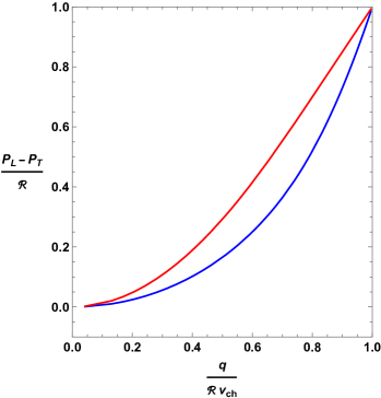
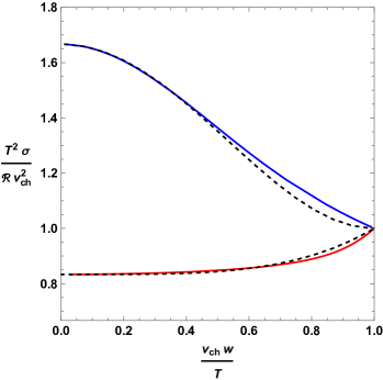
Figure 1: Non-equilibrium thermodynamics of heat conducting fluids according to the Minerbo prescription (blue) and the Levermore prescription (red). Left panel: Pressure anisotropy as a function of the heat flux. Right panel: Transport coefficient $\sigma$ as a function of the non-equilibrium excursion $w$. The dashed lines represent the polynomial fits.

Minerbo: $$\dfrac{P_{L}{-}P_{T}}{\mathfrak{R}} =\dfrac{Z^{2}{-}3Z\coth Z{+}3}{Z^{2}}\;,$$ (18)

Levermore: $$\dfrac{P_{L}{-}P_{T}}{\mathfrak{R}} =\dfrac{3\coth Z(Z\coth Z{-}1)}{2Z}-\dfrac{1}{2}\;.$$ (19)

Plugging these formulas into (13), we obtain two alternative constitutive relations $\sigma(w)$, which are plotted in figure 1, right panel. There is no analytical expression because, in both cases, the relation $\sigma(w)$ is given in a parametric form, $\{w(Z),\sigma(Z)\}$, and the dependence of $w$ on $Z$ does not admit an analytic inverse. However, we can fit the relations using a polynomial approximation. Below, we report a good compromise between analytical simplicity and accuracy (see dashed lines in figure 1):

Minerbo: $$\dfrac{T^{2}\sigma}{\mathfrak{R}v_{\text{ch}}^{2}} =\dfrac{5}{3}-\dfrac{3}{2}\bigg{(}\dfrac{v_{\text{ch}}w}{T}\bigg{)}^{2}+\bigg{(}\dfrac{v_{\text{ch}}w}{T}\bigg{)}^{4}-\dfrac{1}{6}\bigg{(}\dfrac{v_{\text{ch}}w}{T}\bigg{)}^{6}\;,$$ (20)

Levermore: $$\dfrac{T^{2}\sigma}{\mathfrak{R}v_{\text{ch}}^{2}} =\dfrac{5}{6}+\dfrac{1}{6}\bigg{(}\dfrac{v_{\text{ch}}w}{T}\bigg{)}^{4}\;.$$ (21)

These approximations are designed to be very accurate up to $v_{\text{ch}}w/T\sim 0.5$. At larger heat fluxes, the accuracy is slightly lower ($\sim 5$% error). However, at maximum heat flux, namely for $v_{\text{ch}}w/T=1$, the polynomial approximation becomes exact. As a consistency check, we note that, in the limit of small $q$, the conductivity coefficient $\kappa=\tau\sigma T$, as predicted by equation (11), has the correct scaling Tritt (2004) for both models:

$$\kappa\propto\dfrac{\tau\,\mathfrak{R}\,v_{\text{ch}}^{2}}{T}\,.$$ (22)

Using equation (14), we finally obtain the non-equilibrium free energy density for both models (see figure 2):

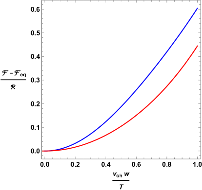
Figure 2: Non-equilibrium part of the free energy density according to Minerbo’s model (blue) and Levermore’s model (red).

Minerbo: $${\mathfrak{F}} ={\mathfrak{F}}_{\text{eq}}+\bigg{[}\dfrac{5}{6}\bigg{(}\dfrac{v_{\text{ch}}w}{T}\bigg{)}^{2}-\dfrac{3}{8}\bigg{(}\dfrac{v_{\text{ch}}w}{T}\bigg{)}^{4}+\dfrac{1}{6}\bigg{(}\dfrac{v_{\text{ch}}w}{T}\bigg{)}^{6}-\dfrac{1}{48}\bigg{(}\dfrac{v_{\text{ch}}w}{T}\bigg{)}^{8}\bigg{]}\mathfrak{R}\;,$$ (23)

Levermore: $${\mathfrak{F}} ={\mathfrak{F}}_{\text{eq}}+\bigg{[}\dfrac{5}{12}\bigg{(}\dfrac{v_{\text{ch}}w}{T}\bigg{)}^{2}+\dfrac{1}{36}\bigg{(}\dfrac{v_{\text{ch}}w}{T}\bigg{)}^{6}\bigg{]}\mathfrak{R}\;.$$ (24)

These are the equations of state we were looking for.

IV Conclusions

At present, we don’t know whether the GM theory is applicable outside of the Israel-Stewart regime. For that to happen, three conditions need to be met. First, the dynamics of heat must be fully characterized by a single non-equilibrium structural variable $w_{\mu}$. Secondly, it should still be possible to define an extended thermodynamic theory involving the non-equilibrium excursion parameter $w^{\mu}w_{\mu}+T^{2}$. Finally, the equation of motion for $w_{\mu}$ should be governed by GENERIC dynamics. And all of this must be true for large values of heat flux. Admittedly, these are quite strong assumptions to digest. However, given the success of GENERIC in describing complex fluids Öttinger (2018), it may happen that certain relativistic liquids indeed fulfill the requirements.

The main danger when dealing with “far-from-equilibrium” theories of this kind is the risk of non-falsifiability. There is so much freedom in the construction of the non-equilibrium equation of state ${\mathfrak{F}}(T,n,w^{\mu}w_{\mu})$ that it is virtually possible to fit any given data a posteriori, by simply adjusting the equation of state to the needs. This would likely result in overfitted fluid models. To avoid this problem, one should know the non-equilibrium equation of state before fitting the data with hydrodynamics. Ideally, the (theoretical) error bars of the non-equilibrium equation of state should be smaller than the (experimental) error bars of the data points.

Here, we have proposed a simple procedure for evaluating ${\mathfrak{F}}(T,n,w^{\mu}w_{\mu})$ for any given microscopic model. This procedure has the advantage of being free of intrinsic uncertainties. Rather than coming up with a statistical interpretation of ${\mathfrak{F}}$, which would suffer from ambiguities related to the unclear microscopic definition of $w_{\mu}$, we adopted a more rigorous approach: We showed that $T$, $w^{\mu}w_{\mu}$, and $\partial{\mathfrak{F}}/\partial(w^{\mu}w_{\mu})$ can all be expressed in terms of physical observables that are unambiguously defined in any kinetic theory. Therefore, if the GM theory holds for large values of $q$ (which is admittedly a big “if”), there is one and only one free energy for each given microscopic model. This makes the GM theory at least falsifiable.

We have tested the method with two simple kinetic models of flux-limited diffusion. The first, due to Minerbo Minerbo (1978), based on the maximum entropy principle, and the second, due to Levermore Levermore (1979); Levermore and Pomraning (1981), based on the Chapman-Enskog procedure Chapman and Cowling (1970). The resulting non-equilibrium free energies are reported in figure 2. Their qualitative behavior is reasonable. For example, the non-equilibrium deviations of the free energy are of the order of the pressure anisotropy, which is rather natural, considering that ${\mathfrak{F}}=\mu n-P$. Indeed, all the scaling laws agree with the expectations.

Appendix A Microscopic derivation of the toy model

A.1 Basic definitions

Our model III.2 describes heat conduction in a quantum liquid, which exhibits different types of weakly interacting elementary excitations (called “branches”), that form an ideal gas. Each type of elementary excitation can be viewed as a quasi-particle Arteaga (2009), and it has an associated dispersion relation. The main working assumption of the model is that all the heat and the pressure anisotropy is carried by a quasi-particle “$Q$” that transports zero net baryon number and has a long mean free path (similarly to what happens in radiation hydrodynamics Weinberg (1971); Udey and Israel (1982)). Thus, if $f_{\textbf{p}}$ is the distribution function of the quasiparticles, we have the following formulas (in the rest frame of $u^{\mu}$) Landau et al. (1980); Pitaevskii and Lifshitz (2012); Popov (2006):

$$\begin{split}q^{j}={}&\int\dfrac{d^{3}p}{(2\pi)^{3}}f_{\textbf{p}}\,\mathfrak{q}^{j}\,,\\ \Delta P^{jk}={}&\int\dfrac{d^{3}p}{(2\pi)^{3}}f_{\textbf{p}}\,\mathfrak{p}^{jk}\,,\\ \end{split}$$ (25)

where $q^{j}$ is the heat flux, and $\Delta P^{jk}$ is the contribution to the stress tensor coming from the quasi-particles $Q$. The vector $\mathfrak{q}^{j}$ and tensor $\mathfrak{p}^{jk}$ are the contributions to respectively the heat flux and the stress tensor coming from a single excitation with momentum $p^{j}$. By isotropy of the background state, we have that $\mathfrak{q}^{j}\propto p^{j}$ and $\mathfrak{p}^{jk}\propto p^{j}p^{k}$.

It is natural, when working within the $M1$ closure scheme, to assume that $f_{\textbf{p}}=f(\Omega)f(\epsilon_{p})$, where $f(\Omega)$ is the normalized angle distribution of the quasi-particles ($\Omega$ is a point on the two-sphere), and $f(\epsilon_{p})$ quantifies how many quasiparticles have energy $\epsilon_{p}$. Therefore, we can split the momentum integral into two separate integrals:

$$\begin{split}q^{j}={}&\int_{4\pi}\dfrac{d^{2}\Omega}{4\pi}\,f(\Omega)\Omega^{j}\int_{0}^{+\infty}\dfrac{p^{2}dp}{2\pi^{2}}f(\epsilon_{p})\mathfrak{q}\,,\\ \Delta P^{jk}={}&\int_{4\pi}\dfrac{d^{2}\Omega}{4\pi}\,f(\Omega)\Omega^{j}\Omega^{k}\int_{0}^{+\infty}\dfrac{p^{2}dp}{2\pi^{2}}f(\epsilon_{p})\mathfrak{p}\,,\\ \end{split}$$ (26)

where $d^{2}\Omega$ is solid-angle element, $\Omega^{j}$ is the unit vector pointing in the direction of $p^{j}$. Let us define the scalars

$$\mathfrak{R}=\int_{0}^{+\infty}\dfrac{p^{2}dp}{2\pi^{2}}f(\epsilon_{p})\mathfrak{p}\,,\quad\quad\quad v_{\text{ch}}=\dfrac{\displaystyle\int_{0}^{+\infty}\dfrac{p^{2}dp}{2\pi^{2}}f(\epsilon_{p})\mathfrak{q}}{\displaystyle\int_{0}^{+\infty}\dfrac{p^{2}dp}{2\pi^{2}}f(\epsilon_{p})\mathfrak{p}}\,.$$ (27)

The first is just the trace $\Delta P\indices{{}^{j}_{j}}$. The interpretation of the second as a velocity comes from the fact that, in the non-relativistic limit, $\mathfrak{q}\sim\epsilon v\sim pv^{2}$, while $\mathfrak{p}\sim pv$ Pitaevskii and Lifshitz (2012). However, we remark that, in relativity, $q^{j}$ may carry also some rest mass, and may be much larger than $\mathfrak{p}$. Thus, relativistic effects may render $v_{\text{ch}}$ larger than one.

Finally, we recall that, in the setting outlined in section III.1, the system is invariant under rotations around the $x^{1}$ axis. Therefore, setting up spherical coordinate such that $\Omega^{1}=\cos\theta$, we can write $f(\Omega)=2f(\cos\theta)$ (the 2 is a normalization constant due to the change of variables), and we obtain

$$\begin{split}q^{j}={}&v_{\text{ch}}\mathfrak{R}\,\delta^{j}_{1}\int_{-1}^{+1}d(\cos\theta)\,f(\cos\theta)\cos\theta\,,\\ \Delta P^{jk}={}&\mathfrak{R}\int_{-1}^{+1}d(\cos\theta)\,f(\cos\theta)\begin{bmatrix}\cos^{2}\theta&0&0\\ 0&\dfrac{1-\cos^{2}\theta}{2}&0\\ 0&0&\dfrac{1-\cos^{2}\theta}{2}\\ \end{bmatrix}\,.\\ \end{split}$$ (28)

Comparison with (12) gives $q=q^{1}$, and $P_{L}-P_{T}=\Delta P^{11}-\Delta P^{22}$, so that

$$\begin{split}&q=v_{\text{ch}}\,\mathfrak{R}\int_{-1}^{+1}d(\cos\theta)f(\cos\theta)\,\cos\theta\,,\\ &P_{L}{-}P_{T}=\mathfrak{R}\int_{-1}^{+1}d(\cos\theta)\,f(\cos\theta)\,\dfrac{3(\cos\theta)^{2}{-}1}{2}\,,\\ \end{split}$$ (29)

in agreement with equation (15).

A.2 Non-equilibrium temperature

If we fix the direction of the heat flux, the hydrodynamic state-space depends on three scalars, namely $\{T,n,w^{\mu}w_{\mu}\}$, see section II.1. Thus, also the distribution $f_{\textbf{p}}=f(\Omega)f(\epsilon_{p})$ should depend on 3 kinetic parameters. In general, we expect the angular distribution $f(\Omega)$ to depend on a single parameter $Z$, which tells us how “anisotropic” the gas is. The energy distribution $f(\epsilon_{p})$, instead, should depend on the density $n$ (since the dispersion relation is density-dependent), and on an additional parameter $W$, which quantifies how much energy is stored in the quasi-particle branch $Q$. In principle, the detailed structure of $f(\epsilon_{p})$ may depend on $Z$, too. However, this should not affect the integrals in (27) appreciably, if $W$ is carefully defined. Thus, we can rewrite (29) in the form

$$\begin{split}&q=v_{\text{ch}}(W,n)\mathfrak{R}(W,n)M_{1}(Z)\,,\\ &P_{L}-P_{T}=\mathfrak{R}(W,n)M_{2}(Z)\,,\\ \end{split}$$ (30)

where $M_{1}$ and $M_{2}$ are the angular integrals in (29). Under these assumptions, we can write a similar formula for the entropy production rate:

$$\tau\nabla_{\mu}s^{\mu}=\mathfrak{S}(W,n)L(Z)\,.$$ (31)

To derive the above equation, one can work in the relaxation-time approximation, see Cercignani and Kremer (2002), equation (8.16), and consider that, in our model setup, most of the dissipation is due to the anisotropy of $f_{\textbf{p}}$, so that

$$\tau\nabla_{\mu}s^{\mu}=\int\dfrac{d^{3}p}{(2\pi)^{3}}f_{\textbf{p}}\,\mathfrak{s}[f_{\textbf{p}}/f_{\text{eq},p}]\approx\int\dfrac{d^{3}p}{(2\pi)^{3}}f_{\textbf{p}}\,\mathfrak{s}[f(\Omega)]=\int_{0}^{+\infty}\dfrac{p^{2}dp}{2\pi^{2}}f(\epsilon_{p})\int_{4\pi}\dfrac{d^{2}\Omega}{4\pi}\,f(\Omega)\mathfrak{s}[f(\Omega)]\,,$$ (32)

where $\mathfrak{s}=\mathfrak{s}[f_{\textbf{p}}/f_{\text{eq},p}]$ is the entropy production per quasi-particle at given $f_{\textbf{p}}/f_{\text{eq},p}$ (with $f_{\text{eq},p}$ being the equilibrium distribution), and it depends on the quantum statistics of the quasi-particles. Thus, we recover (31), with

$$\mathfrak{S}(W,n)=\int_{0}^{+\infty}\dfrac{p^{2}dp}{2\pi^{2}}f(\epsilon_{p})\,,\quad\quad\quad L(Z)=\int_{4\pi}\dfrac{d^{2}\Omega}{4\pi}\,f(\Omega)\mathfrak{s}[f(\Omega)]\,.$$ (33)

Hence, from equation (13), we obtain a formula for the non-equilibrium temperature:

$$T=\dfrac{\mathfrak{R}(W,n)M_{2}(Z)}{\mathfrak{S}(W,n)L(Z)}\,.$$ (34)

The second (and most delicate) working assumption of the model is that the quotient $M_{2}(Z)/L(Z)$ does not depend on $Z$. If that is true, then $T=T(W,n)$, which can be inverted, giving $W=W(T,n)$. As a consequence, $v_{\text{ch}}=v_{\text{ch}}(T,n)$ and $\mathfrak{R}=\mathfrak{R}(T,n)$, and (30) becomes (15).

A.3 Minerbo closure

Now we only need a formula for the dependence of $f(\Omega)$ on $Z$. Minerbo Minerbo (1978) adopted Jaynes’ interpretation of the entropy as missing information Jaynes (1957), and postulated that the most probable distribution $f(\Omega)$, for the given value of $q^{j}$, is the one that maximizes the (Boltzmann) entropy at fixed $q^{j}$. Working with Maxwell-Boltzmann statistics Huang (1987); Landau and Lifshitz (2013), we should therefore require that

$$\delta\!\!\int_{4\pi}\dfrac{d^{2}\Omega}{4\pi}(f\ln f-f-Z_{j}f\Omega^{j}-\lambda f)=0\,,$$ (35)

for any linear variation $\delta f$, at fixed values of the Lagrange multipliers $Z_{j}$ (constraining $q^{j}$) and $\lambda$ (constraining the normalization). After evaluating $\lambda$ explicitly, to guarantee that $f(\Omega)$ is indeed normalised, we obtain

$$f(\Omega)=\dfrac{|\textbf{Z}|e^{Z_{j}\Omega^{j}}}{\sinh(|\textbf{Z}|)}\,.$$ (36)

Setting $Z_{j}=(Z,0,0)$, and recalling that $f(\Omega)=2f(\cos\theta)$, we recover equation (16).

A.4 Levermore closure

The approach of Levermore Levermore (1979); Levermore and Pomraning (1981) is different. The main idea is to approximately solve the Boltzmann equation in the relaxation-time approximation:

$$\dfrac{d}{dl}f_{\textbf{p}}+f_{\textbf{p}}=f_{\text{eq},p}\,,$$ (37)

where $d/dl$ denotes the derivative along the path of the quasi-particle in phase space Pitaevskii and Lifshitz (2012), parameterized in units of the relaxation time. As usual, it is assumed that $f_{\textbf{p}}=f(\epsilon_{p})f(\Omega)$. Additionally, one assumes that $df(\Omega)/dl\approx 0$, because $f(\Omega)$ is expected to be a slowly varying function (compared to $\tau$). This gives

$$f(\Omega)=\dfrac{f_{\text{eq},p}}{f(\epsilon_{p})+df(\epsilon_{p})/dl}\,.$$ (38)

Recalling that we are working in the local rest frame defined by $u^{\mu}$, we see that all the angular dependence of $f(\Omega)$ is encoded in the term $df(\epsilon_{p})/dl$, because both $f_{\text{eq},p}$ and $f(\epsilon_{p})$ are isotropic. Furthermore, it is straightforward to see that the dependence of $df(\epsilon_{p})/dl$ on the vector $\Omega$ comes from terms proportional to $\Omega^{j}\partial_{j}F(\epsilon_{p},T,n)$, for some function $F$. Thus, equation (38) can be rearranged in the abstract form

$$f(\Omega)=\dfrac{1}{\lambda-Z_{j}\Omega^{j}}\,,$$ (39)

where $\lambda$ and $Z_{j}$ do not depend on $\Omega$. Recalling that $f(\Omega)$ is normalised, equation (39) is equivalent to

$$f(\Omega)=\dfrac{1}{|\textbf{Z}|\coth(|\textbf{Z}|)-Z_{j}\Omega^{j}}\,.$$ (40)

Setting $Z_{j}=(Z,0,0)$, and recalling that $f(\Omega)=2f(\cos\theta)$, we recover equation (17).

References

- Israel and Stewart (1979) W. Israel and J. Stewart, Annals of Physics 118, 341 (1979).
- Hiscock and Lindblom (1983) W. A. Hiscock and L. Lindblom, Annals of Physics 151, 466 (1983).
- Denicol et al. (2012) G. S. Denicol, H. Niemi, E. Molnár, and D. H. Rischke, Phys. Rev. D 85, 114047 (2012).
- Gavassino and Antonelli (2023) L. Gavassino and M. Antonelli, Classical and Quantum Gravity 40, 075012 (2023), arXiv:2209.12865 [gr-qc] .
- Jou et al. (1999) D. Jou, J. Casas-Vázquez, and G. Lebon, Reports on Progress in Physics 51, 1105 (1999).
- Cattaneo (1958) C. Cattaneo, Sur une forme de l’équation de la chaleur éliminant le paradoxe d’une propagation instantanée, Comptes rendus hebdomadaires des séances de l’Académie des sciences (Gauthier-Villars, 1958).
- Denicol et al. (2011) G. S. Denicol, J. Noronha, H. Niemi, and D. H. Rischke, Phys. Rev. D 83, 074019 (2011).
- Wagner and Gavassino (2023) D. Wagner and L. Gavassino, (2023), arXiv:2309.14828 [nucl-th] .
- Frenkel (1955) J. Frenkel, Kinetic theory of liquids, 2nd ed. (Dover Publications, New York, 1955).
- Baggioli et al. (2020) M. Baggioli, M. Vasin, V. Brazhkin, and K. Trachenko, Physics Reports 865, 1 (2020), gapped momentum states.
- Gavassino (2023) L. Gavassino, (2023), arXiv:2311.10897 [nucl-th] .
- Levermore and Pomraning (1981) C. D. Levermore and G. C. Pomraning, ApJ 248, 321 (1981).
- Sadowski et al. (2013) A. Sadowski, R. Narayan, A. Tchekhovskoy, and Y. Zhu, MNRAS 429, 3533 (2013), arXiv:1212.5050 [astro-ph.HE] .
- Gavassino et al. (2020) L. Gavassino, M. Antonelli, and B. Haskell, Symmetry 12, 1543 (2020).
- Stephanov and Yin (2018) M. Stephanov and Y. Yin, Phys. Rev. D 98, 036006 (2018), arXiv:1712.10305 [nucl-th] .
- Gavassino et al. (2021) L. Gavassino, M. Antonelli, and B. Haskell, Classical and Quantum Gravity 38, 075001 (2021).
- Gavassino and Noronha (2023) L. Gavassino and J. Noronha, arXiv e-prints , arXiv:2305.04119 (2023), arXiv:2305.04119 [gr-qc] .
- Strickland (2014) M. Strickland, Acta Phys. Polon. B 45, 2355 (2014), arXiv:1410.5786 [nucl-th] .
- Alqahtani et al. (2018) M. Alqahtani, M. Nopoush, and M. Strickland, Prog. Part. Nucl. Phys. 101, 204 (2018), arXiv:1712.03282 [nucl-th] .
- Carter (1989) B. Carter, Covariant theory of conductivity in ideal fluid or solid media, Vol. 1385 (1989) p. 1.
- Carter (1991) B. Carter, Proceedings of the Royal Society of London Series A 433, 45 (1991).
- Lopez-Monsalvo and Andersson (2011) C. S. Lopez-Monsalvo and N. Andersson, Proceedings of the Royal Society of London Series A 467, 738 (2011), arXiv:1006.2978 [gr-qc] .
- Öttinger (1998) H. C. Öttinger, Physica A: Statistical Mechanics and its Applications 259, 24 (1998).
- Grmela and Öttinger (1997) M. Grmela and H. C. Öttinger, Phys. Rev. E 56, 6620 (1997).
- Kovtun (2019) P. Kovtun, Journal of High Energy Physics 2019, 34 (2019), arXiv:1907.08191 [hep-th] .
- Gavassino and Antonelli (2020) L. Gavassino and M. Antonelli, Classical and Quantum Gravity 37, 025014 (2020), arXiv:1906.03140 [gr-qc] .
- Callen (1985) H. B. Callen, Thermodynamics and an introduction to thermostatistics; 2nd ed. (Wiley, New York, NY, 1985).
- Landau and Lifshitz (2013) L. Landau and E. Lifshitz, Statistical Physics, v. 5 (Elsevier Science, 2013).
- Olson and Hiscock (1990) T. S. Olson and W. A. Hiscock, Phys. Rev. D 41, 3687 (1990).
- Priou (1991) D. Priou, Phys. Rev. D 43, 1223 (1991).
- van Kampen (1968) N. G. van Kampen, Phys. Rev. 173, 295 (1968).
- Israel (2009) W. Israel, “Relativistic thermodynamics,” in E.C.G. Stueckelberg, An Unconventional Figure of Twentieth Century Physics: Selected Scientific Papers with Commentaries, edited by J. Lacki, H. Ruegg, and G. Wanders (Birkhäuser Basel, Basel, 2009) pp. 101–113.
- Gavassino (2020) L. Gavassino, Found. Phys. 50, 1554 (2020), arXiv:2005.06396 [gr-qc] .
- Gavassino (2022a) L. Gavassino, Foundations of Physics 52, 11 (2022a), arXiv:2105.09294 [gr-qc] .
- Carter and Khalatnikov (1992) B. Carter and I. M. Khalatnikov, Phys. Rev. D 45, 4536 (1992).
- Gavassino et al. (2022) L. Gavassino, M. Antonelli, and B. Haskell, Phys. Rev. D 105, 045011 (2022).
- Gavassino (2022b) L. Gavassino, Classical and Quantum Gravity 39, 185008 (2022b), arXiv:2202.06760 [gr-qc] .
- Gavassino et al. (2022) L. Gavassino, M. Antonelli, and B. Haskell, Phys. Rev. Lett. 128, 010606 (2022), arXiv:2105.14621 [gr-qc] .
- Gavassino (2021) L. Gavassino, Classical and Quantum Gravity 38, 21LT02 (2021), arXiv:2104.09142 [gr-qc] .
- Kondepudi and Prigogine (2014) D. Kondepudi and I. Prigogine, Modern Thermodynamics (John Wiley and Sons, Ltd, 2014).
- Pathria and Beale (2011) R. Pathria and P. D. Beale, in Statistical Mechanics (Third Edition), edited by R. Pathria and P. D. Beale (Academic Press, Boston, 2011) third edition ed., pp. 583–635.
- Pavelka et al. (2014) M. Pavelka, V. Klika, and M. Grmela, Phys. Rev. E 90, 062131 (2014).
- Gavassino (2022c) L. Gavassino, arXiv e-prints , arXiv:2210.05067 (2022c), arXiv:2210.05067 [nucl-th] .
- Levermore (1984) C. Levermore, Journal of Quantitative Spectroscopy and Radiative Transfer 31, 149 (1984).
- Minerbo (1978) G. N. Minerbo, Journal of Quantitative Spectroscopy and Radiative Transfer 20, 541 (1978).
- Levermore (1979) C. D. Levermore, UCID-18229 (1979).
- Chapman and Cowling (1970) S. Chapman and T. G. Cowling, The Mathematical Theory of Non-Uniform Gases (Cambridge University Press, 1970).
- Tritt (2004) T. Tritt, Thermal Conductivity: Theory, Properties, and Applications (Kluwer Academic/ Plenum Publishers, 2004).
- Öttinger (2018) H. C. Öttinger, arXiv e-prints , arXiv:1810.08470 (2018), arXiv:1810.08470 [cond-mat.soft] .
- Chamel and Haensel (2006) N. Chamel and P. Haensel, Phys. Rev. C 73, 045802 (2006), nucl-th/0603018 .
- Nakano et al. (2020) E. Nakano, K. Iida, and W. Horiuchi, Phys. Rev. C 102, 055802 (2020).
- Liu et al. (2023) H. Liu, Y.-H. Yang, Y. Han, and P.-C. Chu, Phys. Rev. D 108, 034004 (2023), arXiv:2305.01246 [nucl-th] .
- Bluhm et al. (2005) M. Bluhm, B. Kampfer, and G. Soff, Phys. Lett. B 620, 131 (2005), arXiv:hep-ph/0411106 .
- Mykhaylova and Sasaki (2021) V. Mykhaylova and C. Sasaki, Phys. Rev. D 103, 014007 (2021), arXiv:2007.06846 [hep-ph] .
- Li et al. (2023) F.-P. Li, H.-L. Lü, L.-G. Pang, and G.-Y. Qin, Phys. Lett. B 844, 138088 (2023), arXiv:2211.07994 [hep-ph] .
- Arteaga (2009) D. Arteaga, Annals Phys. 324, 920 (2009), arXiv:0801.4324 [hep-ph] .
- Weinberg (1971) S. Weinberg, ApJ 168, 175 (1971).
- Udey and Israel (1982) N. Udey and W. Israel, MNRAS 199, 1137 (1982).
- Landau et al. (1980) L. Landau, E. Lifshitz, and L. Pitaevskij, Statistical Physics: Part 2 : Theory of Condensed State, Landau and Lifshitz Course of theoretical physics (Oxford, 1980).
- Pitaevskii and Lifshitz (2012) L. Pitaevskii and E. Lifshitz, Physical Kinetics, v. 10 (Elsevier Science, 2012).
- Popov (2006) V. Popov, Gen. Rel. Grav. 38, 917 (2006), arXiv:gr-qc/0607023 .
- Cercignani and Kremer (2002) C. Cercignani and G. M. Kremer, The relativistic Boltzmann equation: theory and applications (2002).
- Jaynes (1957) E. T. Jaynes, Phys. Rev. 106, 620 (1957).
- Huang (1987) K. Huang, Statistical Mechanics, 2nd ed. (John Wiley & Sons, 1987).