Sequential Multiuser Scheduling and Power Allocation for Cell-Free Multiple-Antenna Networks

Abstract

Resource allocation is a fundamental task in cell-free (CF) massive multi-input multi-output (MIMO) systems, which can effectively improve the network performance. In this paper, we study the downlink of CF MIMO networks with network clustering and linear precoding, and develop a sequential multiuser scheduling and power allocation scheme. In particular, we present a multiuser scheduling algorithm based on greedy techniques and a gradient ascent (GA) power allocation algorithm for sum-rate maximization when imperfect channel state information (CSI) is considered. Numerical results show the superiority of the proposed sequential scheduling and power allocation scheme and algorithms to existing approaches while reducing the computational complexity and the signaling load.

I Introduction

Cell-free (CF) massive MIMO networks introduced in [1] are distributed massive MIMO networks [2, 3] that include several access points (APs) over a geographic area to serve user equipments (UEs) in the same time and frequency resources, which provides uniform performance across users and improves coverage. Since CF networks in which all UEs are served by all APs, need to process all channels and signals in a central processing unit at the same time, they result in a huge burden to the processors and a substantial increase in costs. Therefore, it is necessary to use clustering techniques, which include network-centric and user-centric approaches [4] to reduce signaling and computational costs.

Resource allocation including power allocation and multiuser scheduling are key tasks for CF networks that can improve the system performance and have attracted a lot of attention in the literature [5, 6, 7, 8, 9, 10, 11, 12, 13, 14, 15, 16, 17, 18, 19, 20, 21, 22]. Multiuser scheduling can reduce multiuser interference in CF networks, improving the system performance. In addition, if the number of receive antennas is larger than those of transmit antennas, it is impossible to support all the receivers which makes it necessary to employ multiuser scheduling. In this context, power allocation also leads to significant performance improvement in CF massive MIMO networks. In [23], the problem of multiuser scheduling, power allocation and beamforming in a user-centric cell-free MIMO wireless system has been solved by maximization of a weighted sum-rate (WSR) problem. The joint optimization of UE scheduling, power allocation and pilot length is investigated in [24] and the minimum ergodic user rate in the downlink transmission is maximized. In [25], the energy efficiency of a user-centric CF massive MIMO system is enhanced by solving a total grid power consumption minimization problem with a joint AP selection and user scheduling algorithm.

In this paper, we consider linear minimum mean square error (MMSE) and zero forcing (ZF) precoders and investigate the downlink of clustered CF massive MIMO networks with multiuser scheduling and power allocation. In particular, we develop a sequential multiuser scheduling and power allocation (SMSPA) scheme based on enhanced greedy and GA techniques to maximize the sum-rate. The proposed enhanced subset greedy (ESG) technique approaches the performance of the optimal exhaustive search method while significant computational cost can be saved. The proposed GA algorithm maximizes the sum-rate and is performed after scheduling the desired UEs set. Simulations show that the proposed SMSPA scheme, ESG and GA algorithms outperform competing approaches.

Notation: Throughout the paper, $\left\|.\right\|_{F}$ denotes the Frobenius norm, $\mathbf{I}_{N}$ denotes the $N\times N$ identity matrix, the complex normal distribution is represented by $\mathcal{CN}\left(.,.\right)$, superscripts ^T, ^∗, and ^H denote transpose, complex conjugate and hermitian operations respectively, $\mathcal{A}\cup\mathcal{B}$ is union of sets $\mathcal{A}$ and $\mathcal{B}$, and $\mathcal{A}\setminus\mathcal{B}$ shows exclusion of set $\mathcal{B}$ from set $\mathcal{A}$.

II System model

The downlink of a CF massive MIMO network is considered where $K$ uniformly distributed single-antenna UEs are supported by $M$ single-antenna APs. Then, the CF network is clustered by dividing the network area into $C$ non-overlapping clusters so that the cluster $c$ includes $K_{c}$ uniformly distributed single-antenna UEs and $M_{c}$ single-antenna APs. We assume that the number of UEs is much larger than the number of APs so that $K>>M$ for the CF network and $K_{c}>>M_{c}$ for cluster $c$ of the clustered CF network, which requires the scheduling of a subset of $n_{c}\leq M_{c}$ UEs per cluster.

II-A Cell-free massive MIMO network and the clustered context

In the CF network, the channel coefficient between AP $m$ and UE $u$ is shown by $g_{m,u}=\sqrt{\beta_{m,u}}h_{m,u}$, [1], including the large scale fading $\beta_{m,u}$ and the small-scale fading $h_{m,u}\sim\mathcal{CN}\left(0,1\right)$ defined as independent and identically distributed (i.i.d.) random variables (RVs) constant during a coherence interval and independent over different coherence intervals. After scheduling $n\leq M$ out of $K$ UEs, the received signal is given by

$$\begin{split}\mathbf{y}&=\sqrt{\rho_{f}}\mathbf{G}^{T}\mathbf{P}\mathbf{x}+\mathbf{w}\\ &=\sqrt{\rho_{f}}\hat{\mathbf{G}}^{T}\mathbf{P}\mathbf{x}+\sqrt{\rho_{f}}\tilde{\mathbf{G}}^{T}\mathbf{P}\mathbf{x}+\mathbf{w}\end{split}$$ (1)

where $\rho_{f}$ is the maximum transmitted power of each antenna, $\mathbf{G}=\hat{\mathbf{G}}+\tilde{\mathbf{G}}$ is the ${M\times n}$ channel matrix, in which $\hat{\mathbf{G}}$ is the channel estimate, $\tilde{\mathbf{G}}$ is the estimation error that models the CSI imperfection and $\left[\mathbf{G}\right]_{m,u}=g_{m,u}$, $m\in\left\{1,\ldots,M\right\}$, $u\in\left\{1,\ldots,n\right\}$, $\mathbf{P}$ is the ${M\times K}$ linear precoder matrix such as MMSE or ZF, $\mathbf{x}=\left[x_{1},\ldots,x_{n}\right]^{T}$ is the zero mean symbol vector with mutually independent elements and independent of the channel coefficients $\mathbf{x}\sim\mathcal{CN}\left(\mathbf{0},\mathbf{I}_{n}\right)$, and $\mathbf{w}=\left[w_{1},\cdots,w_{n}\right]^{T}$ is the additive noise vector with $\mathbf{w}\sim\mathcal{CN}\left(0,\sigma_{w}^{2}\mathbf{I}_{n}\right)$ and statistically independent of the signal vector. We remark that the design of precoders for this system can rely on several strategies [26, 27, 28, 29, 30, 31, 16, 32, 33, 34, 35, 36, 37, 38, 39, 40, 41].

Assuming Gaussian signaling, the sum-rate of the CF system is given by

$$R_{CF}=\log_{2}\left(\det\left[\mathbf{R}+\mathbf{I}_{n}\right]\right),$$ (2)

where the covariance matrix $\mathbf{R}$ is expressed by

$$\mathbf{R}=\rho_{f}\hat{\mathbf{G}}^{T}\mathbf{P}\mathbf{P}^{H}\hat{\mathbf{G}}^{\ast}\left(\rho_{f}\tilde{\mathbf{G}}^{T}\mathbf{P}\mathbf{P}^{H}\tilde{\mathbf{G}}^{\ast}+\sigma_{w}^{2}\mathbf{I}_{n}\right)^{-1}$$ (3)

In the clustered CF network, after scheduling $n_{c}\leq M_{c}$ out of $K_{c}$ UEs, the received signal at cluster $c$ is

$$\begin{split}\mathbf{y}_{c}&=\sqrt{\rho_{f}}\hat{\mathbf{G}}_{cc}^{T}\mathbf{P}_{c}\mathbf{x}_{c}+\sqrt{\rho_{f}}\tilde{\mathbf{G}}_{cc}^{T}\mathbf{P}_{c}\mathbf{x}_{c}\\ &+\sum_{i=1,i\neq c}^{C}\sqrt{\rho_{f}}\hat{\mathbf{G}}_{ic}^{T}\mathbf{P}_{i}\mathbf{x}_{i}+\sum_{i=1,i\neq c}^{C}\sqrt{\rho_{f}}\tilde{\mathbf{G}}_{ic}^{T}\mathbf{P}_{i}\mathbf{x}_{i}+\mathbf{w}_{c}\end{split}$$ (4)

where $\mathbf{G}_{ic}=\hat{\mathbf{G}}_{ic}+\tilde{\mathbf{G}}_{ic}$ is ${M_{i}\times n_{c}}$ channel from APs of the cluster $i$ to the UEs of the cluster $c$, $\mathbf{P}_{i}$ is ${M_{i}\times n_{c}}$ linear precoding matrix, $\mathbf{x}_{i}=\left[x_{i1},\ldots,x_{in_{c}}\right]^{T}$, $\mathbf{x}_{i}\sim\mathcal{CN}\left(\mathbf{0},\mathbf{I}_{n_{c}}\right)$ is the symbol vector of the cluster $i$, $i\in\left\{1,2,\ldots,C\right\}$, and $\mathbf{w}_{c}=\left[w_{c_{1}}\ldots,w_{c_{n_{c}}}\right]^{T}$ is the additive noise vector with $\mathbf{w}_{c}\sim\mathcal{CN}\left(0,\sigma_{w}^{2}\mathbf{I}_{n_{c}}\right)$. Therefore, the sum-rate of the cluster $c$ in this network is given by

$$R_{c}=\log_{2}\left(\det\left[\left(\rho_{f}\hat{\mathbf{G}}_{cc}^{T}\mathbf{P}_{c}\mathbf{P}_{c}^{H}\hat{\mathbf{G}}_{cc}^{*}\right)\mathbf{R}_{c}^{-1}+\mathbf{I}_{n_{c}}\right]\right)$$ (5)

and the covariance matrix $\mathbf{R}_{c}$ is described by

$$\begin{split}\mathbf{R}_{c}&=E\left[\left(\mathbf{y}_{c}-\sqrt{\rho_{f}}\hat{\mathbf{G}}_{cc}^{T}\mathbf{P}_{c}\mathbf{x}_{c}\right)\left(\mathbf{y}_{c}-\sqrt{\rho_{f}}\hat{\mathbf{G}}_{cc}^{T}\mathbf{P}_{c}\mathbf{x}_{c}\right)^{H}\right]\\ &=\rho_{f}\tilde{\mathbf{G}}_{cc}^{T}\mathbf{P}_{c}\mathbf{P}_{c}^{H}\tilde{\mathbf{G}}_{cc}^{*}+\sum_{i=1,i\neq c}^{C}\rho_{f}\hat{\mathbf{G}}_{ic}^{T}\mathbf{P}_{i}\mathbf{P}_{i}^{H}\hat{\mathbf{G}}_{ic}^{*}\\ &+\sum_{i=1,i\neq c}^{C}\rho_{f}\tilde{\mathbf{G}}_{ic}^{T}\mathbf{P}_{i}\mathbf{P}_{i}^{H}\tilde{\mathbf{G}}_{ic}^{*}+\sigma_{w}^{2}\mathbf{I}_{n_{c}}\end{split}$$ (6)

where $\mathbf{x}_{c}$ and $\mathbf{w}_{c}$ are statistically independent. Finally, sum-rate of the total clustered network is given by

$$R_{cl}=\sum_{c=1}^{C}R_{c}.$$ (7)

III Proposed Sequential Multiuser Scheduling and Power Allocation

In this section, we detail the proposed SMSPA scheme for multiuser scheduling and power allocation in clustered CF networks, which is outlined in Fig. 1. In particular, the SMSPA scheme employs an enhanced greedy algorithm for multiuser scheduling using the method presented in [42], in conjunction with a power allocation algorithm based on the GA method to maximize the sum-rate of the network. Unlike the enhanced greedy algorithm of the reference [43] which used equal power loading, we perform both scheduling and power allocation. Specifically, we first consider equal power loading and then employ the proposed greedy multiuser scheduling to schedule the best set using the sum-rate criterion and after that GA power allocation algorithm is employed.

Figure 1: Block diagram of the proposed SMSPA resource allocation.

III-A Proposed ESG multiuser scheduling algorithm

In cluster $c$ including $\mathcal{U}_{c}=\left\{1,\ldots,K_{c}\right\}$ as UEs and $M_{c}$ number of APs ($K_{c}>M_{c}$), in order to schedule a specific number of UEs such as $n_{c}$ so that $n_{c}\leq M_{c}$, we first adapt a greedy method similar to the approach applied in [44] to select the first set of UEs. However, unlike [44] we apply the MMSE precoder instead of the ZF precoder so that we can obtain a better performance and refine the search algorithm. In addition, the number of selected UEs is prespecified. For the selected set $S_{n_{c}}$ which results in a row-reduced channel matrix $\mathbf{G}_{cc}\left(S_{n_{c}}\right)$, we aim at obtaining the solution to the optimization problem

$$\underset{S_{n_{c}}}{\text{max}}~{}R_{MMSE}\left(S_{n_{c}}\right)$$ (8)

$$\text{subject to}\ \left\|\mathbf{P}_{c}\left(S_{n_{c}}\right)\right\|_{F}^{2}\leq P.$$

where $R_{MMSE}\left(S_{n_{c}}\right)$ is defined as the sum-rate with the MMSE precoder when $S_{n_{c}}$ is the set of intended users, $P$ is upper limit to the covariance matrix of the received signal, $\textup{trace}\left[\mathbf{C}_{\mathbf{x}}\right]\leq P$, and $\mathbf{P}_{c}\left(S_{n_{c}}\right)=\mathbf{W}_{c}\mathbf{D}_{c}$ is the precoding matrix including the normalized MMSE weight matrix $\mathbf{W}_{c}\in\mathbb{C}^{M_{c}\times n_{c}}$ and the power allocation matrix $\mathbf{D}_{c}$ defined as

$$\mathbf{D}_{c}=\begin{bmatrix}\sqrt{p_{1}}&0&\cdots&0\\ 0&\sqrt{p_{2}}&\cdots&0\\ \vdots&\vdots&\cdots&\vdots\\ 0&0&\cdots&\sqrt{p_{n_{c}}}\end{bmatrix}=\textup{diag}\left(\mathbf{d}_{c}\right)\\ ,\mathbf{d}_{c}=\left[\sqrt{p_{1}}\ \sqrt{p_{2}}\ \cdots\ \sqrt{p_{n_{c}}}\right]^{T}.$$ (9)

We consider GA power allocation as described in Section III-B and the first set of UEs $S_{{n_{c}}\left(1\right)}$ is obtained using the first stage of Algorithm 1. In order to assess more sets of the users so that we can approach the optimal set achievable by the exhaustive search method, we consider $S_{{n_{c}}\left(2\right)}$ as the second set of UEs which is different from the set $S_{{n_{c}}\left(1\right)}$ in only one UE. To obtain $S_{{n_{c}}\left(2\right)}$, we remove the UE which has the lowest channel power among the UEs of the set $S_{{n_{c}}\left(1\right)}$ shown by $u_{r}$ and replace it with the UE which possesses the most power among the UEs other than the set $S_{{n_{c}}\left(1\right)}$ shown by $u_{a}$. Thus, we can show the removed and added UEs as follows, respectively,

$$u_{r\left(1\right)}=\underset{u\in S_{{n_{c}}\left(1\right)}}{{\arg\min}}~{}\mathbf{g}_{u}^{H}\mathbf{g}_{u}$$ (10)

$$u_{a\left(1\right)}=\underset{u\in\mathcal{U}_{re\left(1\right)}}{{\arg\max}}~{}\mathbf{g}_{u}^{H}\mathbf{g}_{u}$$ (11)

where $\mathbf{g}_{u}=\left[g_{{}_{1,u}}\ \cdots\ g_{{}_{M_{c},u}}\right]^{T}$ is the channel vector to UE $u$, and $\mathcal{U}_{re\left(1\right)}=\mathcal{U}_{c}\setminus S_{{n_{c}}\left(1\right)}$ shows the remaining UE set other than $S_{{n_{c}}\left(1\right)}$. The same process is done for the second set of UEs to find the third set. We continue to find new sets until we obtain $K_{c}-n_{c}$ sets of UEs beside the first set. We obtain the $i$th selected set of UEs and the $i$th remaining set of UEs as follows, respectively,

$$S_{{n_{c}}\left(i\right)}=\left(S_{{n_{c}}\left(i-1\right)}\setminus u_{r\left(i-1\right)}\right)\cup u_{a\left(i-1\right)}$$ (12)

$$\mathcal{U}_{re\left(i\right)}=\mathcal{U}_{re\left(i-1\right)}\setminus u_{a\left(i-1\right)}$$ (13)

where $i\in\left\{2,\cdots,{K_{c}-n_{c}}+1\right\}$. Finally, the desired set $S_{{n_{c}}_{d}}$ among the obtained sets, is the set which results in the highest sum-rate $R_{c}\left(S_{{n_{c}}\left({J}\right)}\right)$, $J\in\left\{1,\cdots,{K_{c}-n_{c}}+1\right\}$ as derived in (5).

1 j=1  % first stage

2       set $l=1$;

3       find a user such that

4      $u_{1}=\underset{u\in\mathcal{U}_{c}}{\textup{argmax}}~{}\mathbf{g}_{u}^{H}\mathbf{g}_{u}$;

5       set $U_{1}={u_{1}}$ and denote the achieved rate

6      $R_{MMSE}\left(U_{1}\right)$;

7

8

Algorithm 1 Proposed C-ESG Scheduling Algorithm.

7       while $l<n_{c}$ do

8                   $l=l+1$;

9                  find a user $u_{l}$ such that

10                  $u_{l}=\underset{u\in\left(\mathcal{U}_{c}\setminus U_{l-1}\right)}{\textup{argmax}}R_{MMSE}\left(U_{l-1}\cup\left\{u\right\}\right)$;

11                  set $U_{l}=U_{l-1}\cup\left\{u_{l}\right\}$ and denote the rate

12                  $R_{MMSE}\left(U_{l}\right)$;

13                  If $R_{MMSE}\left(U_{l}\right)\leq R_{MMSE}\left(U_{l-1}\right)$, break

14                  $l=l-1$;

15       end while

16      $S_{n_{c}\left(\textup{j}\right)}=U_{l}$;

17       compute: $R_{c}\left(S_{n_{c}\left(\textup{j}\right)}\right)$;

18       $\mathcal{U}_{re\left(\textup{j}\right)}=\mathcal{U}_{c}\setminus S_{{n_{c}}\left(\textup{j}\right)}$;

19       $u_{r\left(\textup{j}\right)}=\underset{u\in S_{{n_{c}}\left(\textup{j}\right)}}{\textup{argmin}}\mathbf{g}_{u}^{H}\mathbf{g}_{u}$;

20       $u_{a\left(\textup{j}\right)}=\underset{u\in\mathcal{U}_{re\left(\textup{j}\right)}}{\textup{argmax}}\mathbf{g}_{u}^{H}\mathbf{g}_{u}$;

21      

22

23

24for $\textup{j}=2$ to ${K_{c}-n_{c}}+1$ do

25       $S_{{n_{c}}\left(\textup{j}\right)}=\left(S_{{n_{c}}\left(\textup{j}-1\right)}\setminus u_{r\left(\textup{j}-1\right)}\right)\cup u_{a\left(\textup{j}-1\right)}$;

26       $\mathcal{U}_{re\left(\textup{j}\right)}=\mathcal{U}_{re\left(\textup{j}-1\right)}\setminus u_{a\left(\textup{j}-1\right)}$;

27       $u_{r\left(\textup{j}\right)}=\underset{u\in S_{{n_{c}}\left(\textup{j}\right)}}{\textup{argmin}}\mathbf{g}_{u}^{H}\mathbf{g}_{u}$;

28       $u_{a\left(\textup{j}\right)}=\underset{u\in\mathcal{U}_{re\left(\textup{j}\right)}}{\textup{argmax}}\mathbf{g}_{u}^{H}\mathbf{g}_{u}$;

29       compute: $R_{c}\left(S_{n_{c}\left(\textup{j}\right)}\right)$; 

30 end for

31$S_{{n_{c}}_{d}}=\underset{S_{{n_{c}}}\in S_{{n_{c}}\left({J}\right)}}{\textup{argmax}}\left\{R_{c}\left(S_{{n_{c}}}\right)\right\}$;

Linear MMSE precoding of $n_{c}$ scheduled users

III-B GA power allocation algorithm

In Equation (4), the first part of the right hand side is the desired signal and remaining parts are the terms associated with imperfect CSI, inter-cluster interference and the noise. Therefore, by applying the power allocation, we rewrite the estimated received signal at the cluster $c$ as follows

$$\begin{split}\mathbf{y}_{c}&=\sqrt{\rho_{f}}\hat{\mathbf{G}}_{cc}^{T}\mathbf{W}_{c}\mathbf{D}_{c}\mathbf{x}_{c}+\sqrt{\rho_{f}}\tilde{\mathbf{G}}_{cc}^{T}\mathbf{P}_{c}\mathbf{x}_{c}\\ &+\sum_{i=1,i\neq c}^{C}\sqrt{\rho_{f}}\mathbf{G}_{ic}^{T}\mathbf{P}_{i}\mathbf{x}_{i}+\mathbf{w}_{c}\end{split}$$ (14)

For sum-rate maximization, we combine the received signal of the UEs using a linear receiver $\mathbf{a}=\frac{1}{\sqrt{K_{c}}}\mathbf{1}_{K_{c}}^{T}$, where $\mathbf{1}_{K_{c}}$ is a $1\times K_{c}$ vector of all 1 entities so that $\mathbf{a}^{H}\mathbf{a}=1$ and we obtain a simpler expression for sum-rate [45]. After finding the power loading factors using the simplified sum-rate expression, we apply the obtained power allocation matrix in the sum-rate expressions defined in equations (2) and (5) to determine the sum-rates.

Thus, the combined received signal and the power ratio of the desired part of the signal to the interference and noise (SINR) are given as follows, respectively,

$$\begin{split}\mathbf{a}^{T}\mathbf{y}_{c}&=\sqrt{\rho_{f}}\mathbf{a}^{T}\hat{\mathbf{G}}_{cc}^{T}\mathbf{W}_{c}\mathbf{D}_{c}\mathbf{x}_{c}+\sqrt{\rho_{f}}\mathbf{a}^{T}\tilde{\mathbf{G}}_{cc}^{T}\mathbf{P}_{c}\mathbf{x}_{c}\\ &+\sum_{i=1,i\neq c}^{C}\sqrt{\rho_{f}}\mathbf{a}^{T}\mathbf{G}_{ic}^{T}\mathbf{P}_{i}\mathbf{x}_{i}+\mathbf{a}^{T}\mathbf{w}_{c}\end{split}$$ (15)

$$\textup{SINR}=\frac{\rho_{f}}{\sigma_{w}^{2}}\frac{\mathbf{a}^{T}\hat{\mathbf{G}}_{cc}^{T}\mathbf{W}_{c}\mathbf{D}_{c}\mathbf{D}_{c}^{H}\mathbf{W}_{c}^{H}\hat{\mathbf{G}}_{cc}^{*}\mathbf{a}}{\mathbf{a}^{T}\mathbf{Z}\mathbf{a}}$$ (16)

where

$$\mathbf{Z}=\tilde{\mathbf{G}}_{cc}^{T}\mathbf{P}_{c}\mathbf{P}_{c}^{H}\tilde{\mathbf{G}}_{cc}^{*}+\sum_{i=1,i\neq c}^{C}\rho_{f}{\mathbf{G}}_{ic}^{T}\mathbf{P}_{i}\mathbf{P}_{i}^{H}{\mathbf{G}}_{ic}^{T}+\mathbf{I}$$ (17)

Assuming Gaussian signaling, the rate expression is obtained by $\frac{1}{2}\log_{2}\left(1+\textup{SINR}\right)$. Accordingly, the sum-rate expression is given by

$$SR=\frac{1}{2}\log_{2}\left[1+\frac{\rho_{f}}{\sigma_{w}^{2}}\frac{\mathbf{a}^{T}\hat{\mathbf{G}}_{cc}^{T}\mathbf{W}_{c}\mathbf{D}_{c}\mathbf{D}_{c}^{H}\mathbf{W}_{c}^{H}\hat{\mathbf{G}}_{cc}^{*}\mathbf{a}}{\mathbf{a}^{T}\mathbf{Z}\mathbf{a}}\right].$$ (18)

Equation (18) is similar to $\frac{1}{2}\log_{2}\left(1+bx\right)$ where $b=\frac{\rho_{f}}{\sigma_{w}^{2}\mathbf{a}^{T}\mathbf{Z}\mathbf{a}}$ and $x=\mathbf{a}^{T}\hat{\mathbf{G}}_{cc}^{T}\mathbf{W}_{c}\mathbf{D}_{c}\mathbf{D}_{c}^{H}\mathbf{W}_{c}^{H}\hat{\mathbf{G}}_{cc}^{*}\mathbf{a}$ which is a monotonically increasing function of $x$, $b>0$. Thus, we can maximize $x$ which is equivalent to the sum-rate using the following problem

$$\underset{\mathbf{d}_{c}}{\text{max}}~{}\left(\mathbf{a}^{T}\hat{\mathbf{G}}_{cc}^{T}\mathbf{W}_{c}\textup{diag}\left(\mathbf{d}_{c}\right)\textup{diag}\left(\mathbf{d}_{c}\right)^{H}\mathbf{W}_{c}^{H}\hat{\mathbf{G}}_{cc}^{*}\mathbf{a}\right)$$ (19)

$$\text{subject to}\left\|\mathbf{W}_{c}\textup{diag}\left(\mathbf{d}_{c}\right)\right\|^{2}\leq P.$$

Since the objective function $x$ is scalar, $\textup{trace}(x)=x$. Therefore, by taking the derivative of the objective function with respect to the power loading matrix $\mathbf{D}_{c}$ and using the equality $\frac{\partial\textup{trace}\left(\mathbf{AB}\right)}{\partial\mathbf{A}}=\mathbf{B}\odot\mathbf{I}$ where $\mathbf{A}$ is a diagonal matrix and $\odot$ shows the Hadamard product, we obtain

$$\frac{\partial{x}}{\partial\mathbf{D}_{c}}=2\left(\mathbf{W}_{c}^{H}\hat{\mathbf{G}}_{cc}^{*}\mathbf{a}\mathbf{a}^{T}\hat{\mathbf{G}}_{cc}^{T}\mathbf{W}_{c}\textup{diag}\left(\mathbf{d}_{c}\right)\right)\odot\mathbf{I}$$ (20)

We can use a stochastic GA approach to update the power allocation coefficients as follows

$$\begin{split}\mathbf{d}_{c}\left(i\right)&=\mathbf{d}_{c}\left(i-1\right)+\lambda\frac{\partial{x}}{\partial\mathbf{D}_{c}}=\mathbf{d}_{c}\left(i-1\right)\\ &+2\lambda\left(\mathbf{W}_{c}^{H}\hat{\mathbf{G}}_{cc}^{*}\mathbf{a}\mathbf{a}^{T}\hat{\mathbf{G}}_{cc}^{T}\mathbf{W}_{c}\textup{diag}\left(\mathbf{d}_{c}\left(i-1\right)\right)\right)\odot\mathbf{I}\end{split}$$ (21)

where $i$ and $\lambda$ represent the iteration index and the positive step size, respectively. Before running the adaptive algorithm, the transmit power constraint should be satisfied so that $\left\|\mathbf{W}_{c}\textup{diag}\left(\mathbf{d}_{c}\right)\right\|_{F}^{2}=\left\|\mathbf{P}_{c}\right\|_{F}^{2}\leq P$. Therefore, the power scaling factor $\eta=\sqrt{\frac{\textup{trace}\left(\mathbf{P}_{c}\mathbf{P}_{c}^{H}\right)}{\textup{trace}\left(\mathbf{W}_{c}\textup{diag}\left(\mathbf{d}_{c}.\mathbf{d}_{c}\right)\mathbf{W}_{c}^{H}\right)}}$ is employed in each iteration to scale the coefficients properly. The adaptive power allocation is summarized in Algorithm 2 where $\textup{I}_{t}$ iterations are used. At the receiver, several detection and decoding techniques can be adopted [46, 47, 48, 49, 50, 51, 52, 53, 54, 55, 56, 57, 58, 59, 60, 61, 62, 63, 64, 65, 66, 67, 68, 69, 70, 71].

1 Input $\mathbf{G}_{cc}$, $\mathbf{P}_{c}$, $\mathbf{W}_{c}$, $\ \mathbf{a}$  and   $\lambda$;

2

3$\mathbf{d}_{c}\left(1\right)=\mathbf{0}$;

4

5for ${i}=2$ to $\textup{I}_{t}$ do

6       $\frac{\partial{x}}{\partial\mathbf{D}_{c}}=2\left(\mathbf{W}_{c}^{H}\hat{\mathbf{G}}_{cc}^{*}\mathbf{a}\mathbf{a}^{T}\hat{\mathbf{G}}_{cc}^{T}\mathbf{W}_{c}\textup{diag}\left(\mathbf{d}_{c}\left(i-1\right)\right)\right)\odot\mathbf{I}$;

7       $\mathbf{d}_{c}\left(i\right)=\mathbf{d}_{c}\left({i-1}\right)+\lambda\frac{\partial{x}\left(\varepsilon\right)}{\partial\mathbf{D}_{c}}$;

8      

9      if $\textup{trace}\left(\mathbf{W}_{c}\textup{diag}\left(\mathbf{d}_{c}\left(i\right).\mathbf{d}_{c}\left(i\right)\right)\mathbf{W}_{c}^{H}\right)\neq\textup{trace}\left(\mathbf{P}_{c}\mathbf{P}_{c}^{H}\right)$ then

10             $\eta=\sqrt{\frac{\textup{trace}\left(\mathbf{P}_{c}\mathbf{P}_{c}^{H}\right)}{\textup{trace}\left(\mathbf{W}_{c}\textup{diag}\left(\mathbf{d}_{c}\left(i\right).\mathbf{d}_{c}\left(i\right)\right)\mathbf{W}_{c}^{H}\right)}}$;

11            $\mathbf{d}_{c}\left({i}\right)=\eta\mathbf{d}_{c}\left({i}\right)$;

12       end if

13      

14 end for

15

Algorithm 2 GA Power Allocation Algorithm for Sum-Rate Maximization.

IV SIMULATIONS

In order to assess the proposed SMSPA resource allocation scheme, we compare the sum-rate of the networks that use the proposed ESG, standard greedy (SG), exhaustive search (ES) or WSR user scheduling techniques and the proposed GA power allocation or equal power loading (EPL). Note that we have adapted the WSR technique proposed in [23] to the clustering method we have implemented so that the WSR of the UEs in each cluster supported by the corresponding APs is maximized. The considered CF network is a squared area with the side length of 400 m equipped with $M$ randomly located APs and $K$ uniformly distributed UEs. Applying network-centric clustering, we have considered $C$ = 4 non-overlapping clusters, where cluster c includes $M_{c}$ randomly located APs and $K_{c}$ uniformly distributed UEs and the power allocation is performed using GA algorithm. The large scale coefficient in CF channel coefficient is modeled as $\beta_{m,k}=\textup{PL}_{m,k}\times 10^{\frac{\sigma_{sh}z_{m,k}}{10}}$ where $10^{\frac{\sigma_{sh}z_{m,k}}{10}}$ is the shadow fading with $\sigma_{sh}=8\textup{dB}$, $z_{m,k}\sim\mathcal{N}\left(0,1\right)$, and $\textup{PL}_{m,k}$ is the path loss modeled as [72]

$$\textup{PL}_{m,k}=\left\{\begin{matrix}-\textup{D}-35\log_{10}\left(d_{m,k}\right),\textup{if }d_{m,k}>d_{1}&\\ -\textup{D}-10\log_{10}\left(d_{1}^{1.5}d_{m,k}^{2}\right),\textup{if }d_{0}<d_{m,k}\leq d_{1}&\\ -\textup{D}-10\log_{10}\left(d_{1}^{1.5}d_{0}^{2}\right),\textup{if }d_{m,k}\leq d_{0}&\end{matrix}\right.$$ (22)

where $d_{m,k}$ is the distance between the $m$th AP and $k$th UE and D is

$$\textup{D}=46.3+33.9\log_{10}\left(f\right)-13.82\log_{10}\left(h_{AP}\right)\\ -\left[1.11\log_{10}\left(f\right)-0.7\right]h_{u}+1.56\log_{10}\left(f\right)-0.8$$ (23)

where $f=1900$MHz is the carrier frequency, $h_{AP}=$15m, $h_{u}=$1.5m are the AP and UE antenna heights, respectively, $d_{0}=10$m and $d_{1}=$50m. If $d_{m,k}\leq d_{1}$ there is no shadowing.

In Fig. 2(a), the sum-rate performances of the proposed SMSPA scheme is assessed with the ESG scheduling algorithm using EPL or the GA power allocation when ZF or MMSE precoders are applied. While the sum-rates are increasing with the increase in the signal-to-noise ratio (SNR), the MMSE precoder outperforms the ZF precoder. In addition, the GA power allocation yields significant performance improvement at low-to-medium SNR values.

Fig. 2(b) shows a comparison of different resource allocation techniques when the MMSE precoder is used. We employ a network with a small number of UEs while half of the UEs are scheduled so that we can show the results for the ES method as well as other methods. We notice that the proposed SMSPA resource allocation which has used the ESG and GA algorithms has outperformed other approaches and in the CF network the performance is close to that of the optimal ES method. As expected and according to Equation (4), CF shows better performance than that of the CLCF network because of the extra interference terms caused by other clusters. We clarify that Fig. 2 is plotted according to the sum-rate expressions of equations (2) and (5) and simplified sum-rate equation of (18) is used only to derive the power loading factors. However, as shown in Table I, the computational cost of the proposed SMSPA scheme and the signaling load as the number of channel parameters for CLCF network are substantially lower than CF.

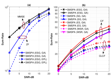
Figure 2: Performance of resource allocation schemes, (a): Comparison of the proposed SMSPA technique in CF networks for ZF and MMSE precoders with the system which has implemented the proposed ESG algorithm and equal power loading (EPL) ($M=64$, $K=128$, $n=24$), (b): Comparison of the different resource allocation techniques in CF and CLCF networks adapting GA power allocation when MMSE precoder is used ($M=64$, $K=16$, $n=8$).

TABLE I: Computational complexity of the proposed SMSPA scheme in floating point operations and the signaling load in parameters for CF and CLCF networks when $M=64$, $K=128$ and $n=64$.

Network	CF	CLCF
Signaling load	24576	6144
Computational cost	$1.3632\times 10^{9}$	$69.354\times 10^{6}$

V CONCLUSIONS

This work has investigated resource allocation and sum-rate performance of the CF and the clustered CF networks with ZF and MMSE precoders. An SMSPA resource allocation scheme is developed that is based on ESG multiuser scheduling and GA power allocation algorithms. Simulations have shown that the proposed SMSPA scheme has outperformed the existing methods and using the PA algorithm has also considerably improved the network performance compared with the EPL case. Additionally, in the case of the network clustering, a substantial computational complexity is saved using the proposed SMSPA scheme and the signaling load is much lower.

References

- [1] H. Q. Ngo, A. Ashikhmin, H. Yang, E. G. Larsson, and T. L. Marzetta, “Cell-free massive mimo versus small cells,” IEEE Transactions on Wireless Communications, vol. 16, no. 3, pp. 1834–1850, 2017.
- [2] R. C. de Lamare, “Massive mimo systems: Signal processing challenges and future trends,” URSI Radio Science Bulletin, vol. 2013, no. 347, pp. 8–20, 2013.
- [3] Wence Zhang, Hong Ren, Cunhua Pan, Ming Chen, Rodrigo C. de Lamare, Bo Du, and Jianxin Dai, “Large-scale antenna systems with ul/dl hardware mismatch: Achievable rates analysis and calibration,” IEEE Transactions on Communications, vol. 63, no. 4, pp. 1216–1229, 2015.
- [4] E. Björnson and L. Sanguinetti, “Scalable cell-free massive mimo systems,” IEEE Transactions on Communications, vol. 68, no. 7, pp. 4247–4261, 2020.
- [5] H. V. Cheng, E. Björnson, and E. G. Larsson, “Optimal pilot and payload power control in single-cell massive mimo systems,” IEEE Transactions on Signal Processing, vol. 65, no. 9, pp. 2363–2378, 2016.
- [6] E. Nayebi, A. Ashikhmin, T. L. Marzetta, and B. D. Rao, “Performance of cell-free massive mimo systems with mmse and lsfd receivers,” in 2016 50th Asilomar Conference on Signals, Systems and Computers. IEEE, 2016, pp. 203–207.
- [7] J. Denis and M. Assaad, “Improving cell-free massive mimo networks performance: A user scheduling approach,” IEEE Transactions on Wireless Communications, vol. 20, no. 11, pp. 7360–7374, 2021.
- [8] V. M. T. Palhares, A. R. Flores, and R. C. de Lamare, “Robust mmse precoding and power allocation for cell-free massive mimo systems,” IEEE Transactions on Vehicular Technology, vol. 70, no. 5, pp. 5115–5120, 2021.
- [9] X. Gong and G. Wu, “Dynamic user scheduling with user satisfaction rate in cell-free massive mimo,” in 2022 IEEE/CIC International Conference on Communications in China (ICCC Workshops). IEEE, 2022, pp. 100–105.
- [10] F. Riera-Palou and G. Femenias, “Trade-offs in cell-free massive mimo networks: Precoding, power allocation and scheduling,” in 2019 14th International Conference on Advanced Technologies, Systems and Services in Telecommunications (TELSIKS). IEEE, 2019, pp. 158–165.
- [11] Patrick Clarke and Rodrigo C. de Lamare, “Joint transmit diversity optimization and relay selection for multi-relay cooperative mimo systems using discrete stochastic algorithms,” IEEE Communications Letters, vol. 15, no. 10, pp. 1035–1037, 2011.
- [12] Patrick Clarke and Rodrigo C. de Lamare, “Transmit diversity and relay selection algorithms for multirelay cooperative mimo systems,” IEEE Transactions on Vehicular Technology, vol. 61, no. 3, pp. 1084–1098, 2012.
- [13] R.C. de Lamare, “Joint iterative power allocation and linear interference suppression algorithms for cooperative ds-cdma networks,” IET Communications, vol. 6, pp. 1930–1942(12), September 2012.
- [14] Yuhan Jiang, Yulong Zou, Haiyan Guo, Theodoros A. Tsiftsis, Manav R. Bhatnagar, Rodrigo C. de Lamare, and Yu-Dong Yao, “Joint power and bandwidth allocation for energy-efficient heterogeneous cellular networks,” IEEE Transactions on Communications, vol. 67, no. 9, pp. 6168–6178, 2019.
- [15] Yunlong Cai, Rodrigo C. de Lamare, and Rui Fa, “Switched interleaving techniques with limited feedback for interference mitigation in ds-cdma systems,” IEEE Transactions on Communications, vol. 59, no. 7, pp. 1946–1956, 2011.
- [16] Jiaqi Gu, Rodrigo C. de Lamare, and Mario Huemer, “Buffer-aided physical-layer network coding with optimal linear code designs for cooperative networks,” IEEE Transactions on Communications, vol. 66, no. 6, pp. 2560–2575, 2018.
- [17] Tong Wang, Rodrigo C. de Lamare, and Anke Schmeink, “Joint linear receiver design and power allocation using alternating optimization algorithms for wireless sensor networks,” IEEE Transactions on Vehicular Technology, vol. 61, no. 9, pp. 4129–4141, 2012.
- [18] Tong Wang, Rodrigo C. de Lamare, and Anke Schmeink, “Alternating optimization algorithms for power adjustment and receive filter design in multihop wireless sensor networks,” IEEE Transactions on Vehicular Technology, vol. 64, no. 1, pp. 173–184, 2015.
- [19] Yunlong Cai, Rodrigo C. de Lamare, Lie-Liang Yang, and Minjian Zhao, “Robust mmse precoding based on switched relaying and side information for multiuser mimo relay systems,” IEEE Transactions on Vehicular Technology, vol. 64, no. 12, pp. 5677–5687, 2015.
- [20] Flavio L. Duarte and Rodrigo C. de Lamare, “Switched max-link relay selection based on maximum minimum distance for cooperative mimo systems,” IEEE Transactions on Vehicular Technology, vol. 69, no. 2, pp. 1928–1941, 2020.
- [21] Xiaotao Lu and Rodrigo C. de Lamare, “Opportunistic relaying and jamming based on secrecy-rate maximization for multiuser buffer-aided relay systems,” IEEE Transactions on Vehicular Technology, vol. 69, no. 12, pp. 15269–15283, 2020.
- [22] André R. Flores and Rodrigo C. de Lamare, “Robust and adaptive power allocation techniques for rate splitting based mu-mimo systems,” IEEE Transactions on Communications, vol. 70, no. 7, pp. 4656–4670, 2022.
- [23] H. A. Ammar, R. Adve, S. Shahbazpanahi, G. Boudreau, and K. V. Srinivas, “Downlink resource allocation in multiuser cell-free mimo networks with user-centric clustering,” IEEE Transactions on Wireless Communications, 2021.
- [24] Y. Ming, Z. Sha, Y. Dong, and Z. Wang, “Downlink resource allocation with pilot length optimization for user-centric cell-free mimo networks,” IEEE Communications Letters, 2022.
- [25] R. Hamdi and M. Qaraqe, “Power allocation and cooperation in cell-free massive mimo systems with energy exchange capabilities,” in 2020 IEEE 91st Vehicular Technology Conference (VTC2020-Spring). IEEE, 2020, pp. 1–5.
- [26] Keke Zu, Rodrigo C. de Lamare, and Martin Haardt, “Generalized design of low-complexity block diagonalization type precoding algorithms for multiuser mimo systems,” IEEE Transactions on Communications, vol. 61, no. 10, pp. 4232–4242, 2013.
- [27] Keke Zu, Rodrigo C. de Lamare, and Martin Haardt, “Multi-branch tomlinson-harashima precoding design for mu-mimo systems: Theory and algorithms,” IEEE Transactions on Communications, vol. 62, no. 3, pp. 939–951, 2014.
- [28] Lukas T. N. Landau and Rodrigo C. de Lamare, “Branch-and-bound precoding for multiuser mimo systems with 1-bit quantization,” IEEE Wireless Communications Letters, vol. 6, no. 6, pp. 770–773, 2017.
- [29] Keke Zu and Rodrigo C. de Lamare, “Low-complexity lattice reduction-aided regularized block diagonalization for mu-mimo systems,” IEEE Communications Letters, vol. 16, no. 6, pp. 925–928, 2012.
- [30] Wence Zhang, Rodrigo C. de Lamare, Cunhua Pan, Ming Chen, Jianxin Dai, Bingyang Wu, and Xu Bao, “Widely linear precoding for large-scale mimo with iqi: Algorithms and performance analysis,” IEEE Transactions on Wireless Communications, vol. 16, no. 5, pp. 3298–3312, 2017.
- [31] Cornelius T. Healy and Rodrigo C. de Lamare, “Design of ldpc codes based on multipath emd strategies for progressive edge growth,” IEEE Transactions on Communications, vol. 64, no. 8, pp. 3208–3219, 2016.
- [32] Tong Peng and Rodrigo C. de Lamare, “Adaptive buffer-aided distributed space-time coding for cooperative wireless networks,” IEEE Transactions on Communications, vol. 64, no. 5, pp. 1888–1900, 2016.
- [33] Lei Zhang, Yunlong Cai, Rodrigo C. de Lamare, and Minjian Zhao, “Robust multibranch tomlinson–harashima precoding design in amplify-and-forward mimo relay systems,” IEEE Transactions on Communications, vol. 62, no. 10, pp. 3476–3490, 2014.
- [34] Andre R. Flores, Rodrigo C. de Lamare, and Bruno Clerckx, “Linear precoding and stream combining for rate splitting in multiuser mimo systems,” IEEE Communications Letters, vol. 24, no. 4, pp. 890–894, 2020.
- [35] Andre R. Flores, Rodrigo C. De Lamare, and Bruno Clerckx, “Tomlinson-harashima precoded rate-splitting with stream combiners for mu-mimo systems,” IEEE Transactions on Communications, vol. 69, no. 6, pp. 3833–3845, 2021.
- [36] Andre R. Flores, Rodrigo C. de Lamare, and Kumar Vijay Mishra, “Clustered cell-free multi-user multiple-antenna systems with rate-splitting: Precoder design and power allocation,” IEEE Transactions on Communications, vol. 71, no. 10, pp. 5920–5934, 2023.
- [37] Yunlong Cai, Rodrigo C. de Lamare, and Didier Le Ruyet, “Transmit processing techniques based on switched interleaving and limited feedback for interference mitigation in multiantenna mc-cdma systems,” IEEE Transactions on Vehicular Technology, vol. 60, no. 4, pp. 1559–1570, 2011.
- [38] Victoria M. T. Palhares, Andre R. Flores, and Rodrigo C. de Lamare, “Robust mmse precoding and power allocation for cell-free massive mimo systems,” IEEE Transactions on Vehicular Technology, vol. 70, no. 5, pp. 5115–5120, 2021.
- [39] Lukas T. N. Landau, Meik Dörpinghaus, Rodrigo C. de Lamare, and Gerhard P. Fettweis, “Achievable rate with 1-bit quantization and oversampling using continuous phase modulation-based sequences,” IEEE Transactions on Wireless Communications, vol. 17, no. 10, pp. 7080–7095, 2018.
- [40] Silvio F. B. Pinto and Rodrigo C. de Lamare, “Block diagonalization precoding and power allocation for multiple-antenna systems with coarsely quantized signals,” IEEE Transactions on Communications, vol. 69, no. 10, pp. 6793–6807, 2021.
- [41] Hajar El Hassani, Anne Savard, E. Veronica Belmega, and Rodrigo C. de Lamare, “Multi-user downlink noma systems aided by ambient backscattering: Achievable rate regions and energy-efficiency maximization,” IEEE Transactions on Green Communications and Networking, vol. 7, no. 3, pp. 1135–1148, 2023.
- [42] S. Mashdour, R. C. De Lamare, and J. P. S. Lima, “Enhanced subset greedy multiuser scheduling in clustered cell-free massive mimo systems,” IEEE Communications Letters, 2022.
- [43] S. Mashdour, R. C. de Lamare, and J. P. S. H. Lima, “Multiuser scheduling with enhanced greedy techniques for multicell and cell-free massive mimo systems,” 2022 IEEE 95th Vehicular Technology Conference:(VTC2022-Spring), pp. 1–5, 2022.
- [44] G. Dimic and N. D. Sidiropoulos, “On downlink beamforming with greedy user selection: performance analysis and a simple new algorithm,” IEEE Transactions on Signal processing, vol. 53, no. 10, pp. 3857–3868, 2005.
- [45] T. Wang, R. C. de Lamare, and A. Schmeink, “Joint linear receiver design and power allocation using alternating optimization algorithms for wireless sensor networks,” IEEE transactions on vehicular technology, vol. 61, no. 9, pp. 4129–4141, 2012.
- [46] Rodrigo C. de Lamare and Raimundo Sampaio-Neto, “Adaptive reduced-rank processing based on joint and iterative interpolation, decimation, and filtering,” IEEE Transactions on Signal Processing, vol. 57, no. 7, pp. 2503–2514, 2009.
- [47] Rodrigo C. De Lamare and Raimundo Sampaio-Neto, “Minimum mean-squared error iterative successive parallel arbitrated decision feedback detectors for ds-cdma systems,” IEEE Transactions on Communications, vol. 56, no. 5, pp. 778–789, 2008.
- [48] Peng Li, Rodrigo C. de Lamare, and Rui Fa, “Multiple feedback successive interference cancellation detection for multiuser mimo systems,” IEEE Transactions on Wireless Communications, vol. 10, no. 8, pp. 2434–2439, 2011.
- [49] R. Fa, “Multi-branch successive interference cancellation for mimo spatial multiplexing systems: design, analysis and adaptive implementation,” IET Communications, vol. 5, pp. 484–494(10), March 2011.
- [50] Peng Li and Rodrigo C. De Lamare, “Adaptive decision-feedback detection with constellation constraints for mimo systems,” IEEE Transactions on Vehicular Technology, vol. 61, no. 2, pp. 853–859, 2012.
- [51] Rodrigo C. de Lamare and Raimundo Sampaio-Neto, “Adaptive reduced-rank equalization algorithms based on alternating optimization design techniques for mimo systems,” IEEE Transactions on Vehicular Technology, vol. 60, no. 6, pp. 2482–2494, 2011.
- [52] Rodrigo C. de Lamare and Raimundo Sampaio-Neto, “Reduced-rank space–time adaptive interference suppression with joint iterative least squares algorithms for spread-spectrum systems,” IEEE Transactions on Vehicular Technology, vol. 59, no. 3, pp. 1217–1228, 2010.
- [53] Rodrigo C. de Lamare, “Adaptive and iterative multi-branch mmse decision feedback detection algorithms for multi-antenna systems,” IEEE Transactions on Wireless Communications, vol. 12, no. 10, pp. 5294–5308, 2013.
- [54] Andre G. D. Uchoa, Cornelius T. Healy, and Rodrigo C. de Lamare, “Iterative detection and decoding algorithms for mimo systems in block-fading channels using ldpc codes,” IEEE Transactions on Vehicular Technology, vol. 65, no. 4, pp. 2735–2741, 2016.
- [55] Zhichao Shao, Rodrigo C. de Lamare, and Lukas T. N. Landau, “Iterative detection and decoding for large-scale multiple-antenna systems with 1-bit adcs,” IEEE Wireless Communications Letters, vol. 7, no. 3, pp. 476–479, 2018.
- [56] Hang Ruan and Rodrigo C. de Lamare, “Robust adaptive beamforming using a low-complexity shrinkage-based mismatch estimation algorithm,” IEEE Signal Processing Letters, vol. 21, no. 1, pp. 60–64, 2014.
- [57] Hang Ruan and Rodrigo C. de Lamare, “Robust adaptive beamforming based on low-rank and cross-correlation techniques,” IEEE Transactions on Signal Processing, vol. 64, no. 15, pp. 3919–3932, 2016.
- [58] Hang Ruan and Rodrigo C. de Lamare, “Robust adaptive beamforming based on low-rank and cross-correlation techniques,” IEEE Transactions on Signal Processing, vol. 64, no. 15, pp. 3919–3932, 2016.
- [59] Tong Wang, Rodrigo C. de Lamare, and Paul D. Mitchell, “Low-complexity set-membership channel estimation for cooperative wireless sensor networks,” IEEE Transactions on Vehicular Technology, vol. 60, no. 6, pp. 2594–2607, 2011.
- [60] Nuan Song, Rodrigo C. de Lamare, Martin Haardt, and Mike Wolf, “Adaptive widely linear reduced-rank interference suppression based on the multistage wiener filter,” IEEE Transactions on Signal Processing, vol. 60, no. 8, pp. 4003–4016, 2012.
- [61] Jingjing Liu and Rodrigo C. de Lamare, “Low-latency reweighted belief propagation decoding for ldpc codes,” IEEE Communications Letters, vol. 16, no. 10, pp. 1660–1663, 2012.
- [62] Peng Li and Rodrigo C. de Lamare, “Distributed iterative detection with reduced message passing for networked mimo cellular systems,” IEEE Transactions on Vehicular Technology, vol. 63, no. 6, pp. 2947–2954, 2014.
- [63] Yunlong Cai, Rodrigo C. de Lamare, Benoit Champagne, Boya Qin, and Minjian Zhao, “Adaptive reduced-rank receive processing based on minimum symbol-error-rate criterion for large-scale multiple-antenna systems,” IEEE Transactions on Communications, vol. 63, no. 11, pp. 4185–4201, 2015.
- [64] Zhichao Shao, Lukas T. N. Landau, and Rodrigo C. de Lamare, “Dynamic oversampling for 1-bit adcs in large-scale multiple-antenna systems,” IEEE Transactions on Communications, vol. 69, no. 5, pp. 3423–3435, 2021.
- [65] Roberto B. Di Renna and Rodrigo C. de Lamare, “Adaptive activity-aware iterative detection for massive machine-type communications,” IEEE Wireless Communications Letters, vol. 8, no. 6, pp. 1631–1634, 2019.
- [66] Roberto B. Di Renna and Rodrigo C. de Lamare, “Iterative list detection and decoding for massive machine-type communications,” IEEE Transactions on Communications, vol. 68, no. 10, pp. 6276–6288, 2020.
- [67] Roberto B. Di Renna, Carsten Bockelmann, Rodrigo C. de Lamare, and Armin Dekorsy, “Detection techniques for massive machine-type communications: Challenges and solutions,” IEEE Access, vol. 8, pp. 180928–180954, 2020.
- [68] Zhichao Shao, Lukas T. N. Landau, and Rodrigo C. De Lamare, “Channel estimation for large-scale multiple-antenna systems using 1-bit adcs and oversampling,” IEEE Access, vol. 8, pp. 85243–85256, 2020.
- [69] Roberto B. Di Renna and Rodrigo C. de Lamare, “Dynamic message scheduling based on activity-aware residual belief propagation for asynchronous mmtc,” IEEE Wireless Communications Letters, vol. 10, no. 6, pp. 1290–1294, 2021.
- [70] Roberto B. Di Renna and Rodrigo C. de Lamare, “Joint channel estimation, activity detection and data decoding based on dynamic message-scheduling strategies for mmtc,” IEEE Transactions on Communications, vol. 70, no. 4, pp. 2464–2479, 2022.
- [71] Ana Beatriz L. B. Fernandes, Zhichao Shao, Lukas T. N. Landau, and Rodrigo C. de Lamare, “Multiuser-mimo systems using comparator network-aided receivers with 1-bit quantization,” IEEE Transactions on Communications, vol. 71, no. 2, pp. 908–922, 2023.
- [72] A. Tang, J. Sun, and K. Gong, “Mobile propagation loss with a low base station antenna for nlos street microcells in urban area,” in IEEE VTS 53rd Vehicular Technology Conference, Spring 2001. Proceedings (Cat. No. 01CH37202). IEEE, 2001, vol. 1, pp. 333–336.