Quantum electrodynamics under a quench

Abstract

Quantum electrodynamics (QED) is a cornerstone of particle physics and also finds diverse applications in condensed matter systems. Despite its significance, the dynamics of quantum electrodynamics under a quantum quench remains inadequately explored. In this paper, we investigate the nonequilibrium regime of quantum electrodynamics following a global quantum quench. Specifically, a massive Dirac fermion is quenched to a gapless state with an interaction with gauge bosons. In stark contrast to equilibrium (3+1)-dimensional QED with gapless Dirac fermions, where the coupling is marginally irrelevant, we identify a nonequilibrium fixed point characterized by non-Fermi liquid behavior. Notably, the anomalous dimension at this fixed point varies with the initial quench parameter, suggesting an interesting quantum memory effect in a strongly interacting system. Additionally, we propose distinctive experimental signatures for nonequilibrium quantum electrodynamics.

Introduction.— In recent years, the progress of experiment platforms like the ion trap systems [1, 2, 3] and cold atom systems [4, 5] has provided people with programmable and highly coherent many-body quantum systems with abundant exotic physics. These developments have also facilitated the exploration of nonequilibrium physics in correlated quantum systems [6, 7, 8, 9, 10]. In addition, pump-probe spectroscopy of correlated materials [11, 12] provides methods to drive the quantum many-body system far away from equilibrium, such as performing a sudden quench to the Hamiltonian parameters [1, 13]. The postquench quantum dynamics can exhibit fruitful non-trivial behaviors that are distinguished from the well-studied equilibrium systems. It is well known that an isolated quantum many-body system that satisfies the eigenstate thermalization hypothesis [14, 15] (ETH) is expected to thermalize, and lose the memory of its initial state [1, 16]. However, additional universal initial information other than the conserved quantities can be preserved for a long time in some exotic prethermal states [17, 18, 19, 20, 21, 22, 23, 24, 25, 26, 27, 28, 29, 30]. One such exotic phenomenon is the quantum memory phenomena [31, 32] which is widespread in different areas of physics. To understand these non-thermal behaviors, various cases have been studied and analyzed, including the proximity to integratibility [33, 34, 35, 36, 37, 38, 39], non-thermal fixed point [40, 41, 42, 43, 44, 45, 46, 47, 48, 49, 50, 51, 52], quenched induced dynamical phase transition [53, 54, 55, 56, 57, 58, 59, 60, 61, 62, 63, 64, 65, 66, 67, 68].

Gapless Dirac fermion is a basic description of the low-energy excitations in various equilibrium condensed matter systems including Dirac semimetals, graphene, and surface modes of the topological insulators [69, 70]. Though exotic quantum phase transitions have been explored for the equilibrium Dirac fermions, the dynamical phase transition remains mysterious. A previous study has revealed the universal prethermal dynamics of a Dirac system coupled to a bosonic field by Yukawa coupling [24]. Their study identified the unique non-equilibrium behaviors of the Dirac gapless fermions. On the other hand, when coupled to gauge bosons, the Dirac fermion system realizes quantum electrodynamics (QED). QED is one of the most successful theories in particle physics [71]. Furthermore, it has found applications in condensed matter physics, including the study of high-temperature superconductors [72, 73], graphene [74, 75, 76, 77, 78], Weyl semimetals [79, 80, 81], and fractional quantum anomalous Hall system [82, 83]. However, the quenching dynamics of QED remains an open question.

In this letter, we investigate the prethermal and nonequilibrium behavior of QED. More explicitly, a Dirac fermion with $U(1)$ gauge bosons after a quench to a critical point, where the Dirac fermion becomes gapless, is studied. Using the Keldysh renormalization group [84] and calculating the perturbation up to the leading order, we find that, on a long timescale, the 2+1 and 3+1 dimensional QED exhibits fixed points distinguished from the equilibrium ones. In 3+1 dimensions, we identify a nontrivial fix point with non-Fermi liquid behaviors. At this nontrivial fixed point, the anomalous dimension of the Dirac fermion depends on the initial quench parameter, indicating a quantum memory effect. This is in stark contrast to the equilibrium QED, in which the interaction is marginally irrelevant. We also propose the differential conductance as a unique experimental signature of such a non-Fermi liquid behavior. On the other hand, in the 2+1 dimensions, we find that the quenched QED eventually flows to a non-interacting theory, which is also different from the equilibrium QED₃. In the following, we focus on the investigation of 3+1 dimensional QED, and leave the discussion of 2+1 dimensional QED to the Appendix.

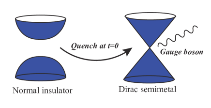
Figure 1: A schematic plot of the quench from a normal insulator phase to a Dirac semimetal phase at time $t=0$.

Feynman propagators after a sudden quench.— To study the prethermal behavior of quantum electrodynamics, we consider a quench of a free massive Dirac fermion with mass $m$ at temperature $\beta$ to a massless Dirac fermion at time zero that couples to a $U(1)$ gauge field as shown in the Fiq. 1. The dynamics of free Dirac fermion in the imaginary-time evolution and real-time evolution are then described by the Hamiltonians

$$H_{E}=\bm{k}\cdot\bm{\alpha}+m\gamma^{0},\quad H_{R}=\bm{k}\cdot\bm{\alpha},$$ (1)

where the subscript $E$ and $R$ refer to the Euclidean evolution and real-time evolution, respectively. We will also call them prequench and postquench (free) Hamiltonian. ${\bm{k}}\equiv(k_{x},k_{y},k_{z})$ and $m$ are the momentum and mass of the Dirac fermion, respectively. Note that the postquench Dirac fermion is massless. $\gamma^{\mu},\mu=0,1,2,3$ denotes the Dirac matrix that satisfies $\{\gamma^{\mu},\gamma^{\nu}\}=2g^{\mu\nu}$. Here, we use the convention $g_{\mu\nu}=\text{diag}(1,-1,-1,-1)$. ${\bm{\alpha}}$ is defined via ${\bm{\alpha}}\equiv(\gamma^{0}\gamma^{1},\gamma^{0}\gamma^{2},\gamma^{0}\gamma^{3})$. Such a quench protocol can be realized in numerous condensed matter systems. For instance, it describes a sudden change of parameters that brings normal insulators to a Dirac semimetal phase, or describes a sudden quench to the normal insulator/topological insulator transition point.

The Keldysh contour of the imaginary-time and the real-time evolution is illustrated in Fig. 2. It is convenient to apply a conventional Keldysh rotation defined by

$$\psi_{c/q}=\frac{1}{\sqrt{2}}(\psi_{+}\pm\psi_{-}),\quad\psi_{c/q}^{\dagger}=\frac{1}{\sqrt{2}}(\psi_{+}^{\dagger}\mp\psi_{-}^{\dagger}),$$ (2)

and work in the Keldysh rotated field in the real-time evolution contour. To obtain the Keldysh propagators, it is convenient to define the projector

$$P_{\pm}(m) =\frac{1}{2}\left(1\pm(\bm{\hat{k}}_{m}\cdot\bm{\alpha}+\hat{m}\gamma^{0})\right),$$ (3)

$$H_{E}P_{\pm}(m) =\pm\xi P_{\pm}(m),\quad H_{R}P_{\pm}=\pm|\bm{k}|P_{\pm},$$

where $\bm{\hat{k}}_{m}=\xi^{-1}(k_{x},k_{y},k_{z}),\quad\hat{m}=\xi^{-1}m,\quad\xi\equiv\sqrt{\bm{k}^{2}+m^{2}}$ and $P_{\pm}\equiv P_{\pm}(0)$. To proceed, we solve the equation of motion with the free Hamiltonian Eq. 1 in the Keldysh contour. Note that it can be done by solving the field variable and then matching the boundary conditions at $\tau=0$ and $\tau=\beta$. For details, one can refer to the Appendix.

With the knowledge of the solution, one can obtain the Keldysh propagator at the real-time contour that characterizes the quench protocol

$$\langle\Psi(t_{1})\bar{\Psi}(t_{2})\rangle =\mathfrak{i}\left(\begin{array}[]{cccc}G_{R}&G_{K}\\ 0&G_{A}\end{array}\right)(t_{1},t_{2}),$$ (4)

$$\mathfrak{i}G_{K}(t_{1},t_{2};\bm{k}) =\tanh\frac{\beta\xi}{2}(e^{-\mathfrak{i}|\bm{k}|t_{1}}P_{+}+e^{\mathfrak{i}|\bm{k}|t_{1}}P_{-})\times$$

$$(P_{+}(m)-P_{-}(m))(e^{\mathfrak{i}|\bm{k}|t_{2}}P_{+}+e^{-\mathfrak{i}|\bm{k}|t_{2}}P_{-})\gamma^{0},$$

where $\Psi\equiv(\psi_{c},\psi_{q})^{T}$, $\bar{\psi}=\psi^{\dagger}\gamma^{0}$. The quench parameter $m$ breaks the time translation symmetry of $G_{K}$, while other propagators are conventional

$$\mathfrak{i}G_{R/A}(t;\bm{k})=\pm\theta(\pm t)\left(e^{-\mathfrak{i}|\bm{k}|t}P_{+}+e^{\mathfrak{i}|\bm{k}|t}P_{-}\right)\gamma^{0},$$ (5)

where $\theta$ denotes the step function.

The $U(1)$ gauge fields coupled to the fermion can be described by the action:

$$S =\frac{1}{4}\int F_{\mu\nu}F^{\mu\nu},$$ (6)

where $F_{\mu\nu}=\partial_{\mu}A_{\nu}-\partial_{\nu}A_{\mu}$ is the field strength tensor. For later convenience, we can also apply the Keidysh rotation for gauge bosons:

$$A_{c/q}=\frac{1}{\sqrt{2}}(A_{+}\pm A_{-}).$$ (7)

Then, after gauge fixing, we obtain the gauge boson propagator in the classical/quantum fields basis,

$$\hat{D}_{\mu\nu}(t,\bm{k})=\mathfrak{i}\left(\begin{array}[]{cccc}D^{K}_{\mu\nu}&D^{R}_{\mu\nu}\\ D^{A}_{\mu\nu}&0\end{array}\right)(t,\bm{k}),$$ (8)

with

$$D_{\mu\nu}^{R}(t,\bm{k}) =-\mathfrak{i}\langle A_{c,\mu}(t)A_{q,\nu}(0)\rangle=\theta(t)g_{\mu\nu}\frac{\sin(|\bm{k}|t)}{|\bm{k}|},$$ (9)

$$D_{\mu\nu}^{A}(t,\bm{k}) =-\mathfrak{i}\langle A_{q,\mu}(t)A_{c,\nu}(0)\rangle=-\theta(-t)g_{\mu\nu}\frac{\sin(|\bm{k}|t)}{|\bm{k}|},$$

$$D_{\mu\nu}^{K}(t,\bm{k}) =-\mathfrak{i}\langle A_{c,\mu}(t)A_{c,\nu}(0)\rangle=\mathfrak{i}g_{\mu\nu}\coth\frac{\beta|\bm{k}|}{2}\frac{\cos(|\bm{k}|t)}{|\bm{k}|}.$$

One can see that, since the information of the quench protocol is encoded in the fermion Keldysh propagator, only the Keldysh propagator 4 breaks time translation symmetry. In the following, we work at zero temperature $\beta\rightarrow\infty$.

Figure 2: A schematic contour of the quench dynamics. The vertical (horizontal) line denotes the imaginary-time (real-time Keldysh) evolution.

Effective action and Ward identity.— The quench protocol explicitly breaks the time translation symmetry but preserves the space translation symmetry, so unlike the ordinary QED, the Lorentz symmetry is broken. Without Lorentz symmetry, the time and space component couplings can be different in general. To account for this space and time anisotropy, the effective action is generalized to be

$$S =S_{0}+S_{\text{int}},$$ (10)

$$S_{0} =\int_{0}^{\infty}dt\int_{\bm{x}}\bar{\Psi}\left(\begin{array}[]{cccc}\mathfrak{i}\partial_{\mu}\gamma^{\mu}&0\\ 0&\mathfrak{i}\partial_{\mu}\gamma^{\mu}\end{array}\right)\Psi+\int_{0}^{\infty}dt\int_{\bm{x}}A_{c,q}\left(g^{\mu\nu}\partial^{2}-\partial^{\mu}\partial^{\nu}\right)A_{q,\nu},$$

$$S_{\text{int}} =\frac{1}{\sqrt{2}}\int_{0}^{\infty}dt\int_{\bm{x}}\left(e_{c}\bar{\Psi}A_{c,0}\gamma^{0}\Psi+g_{c}\bar{\Psi}A_{c,i}\gamma^{i}\Psi+e_{q}\bar{\Psi}A_{q,0}\rho^{x}\gamma^{0}\Psi+g_{q}\bar{\Psi}A_{q,i}\rho^{x}\gamma^{i}\Psi\right),$$

where $\int_{\bm{x}}\equiv\int d^{3}x$, $e_{c,q}$ and $g_{c,q}$ denote the gauge coupling for the time and space component, and $\rho^{x}$ is the Pauli matrix acting on the Keldysh space. The broken Lorentz symmetry allows $e_{c,q}$ and $g_{c,q}$ to flow differently in the RG flow. We also allow the light velocity to flow, which amounts to rescaling $\partial_{i}\rightarrow c\partial_{i}$.

An important consequence of gauge symmetry is the Ward identity. In the quench dynamics, special attention should be paid to the boundary at time $t=0$. Under the transformation for arbitrary spacetime dependent variable $\theta(x)$, i.e., $\Psi\rightarrow e^{\mathfrak{i}\theta}\Psi$, the theory is invariant. This leads to the Ward identity,

$$\delta(t-t_{1})\mathfrak{i}G(t_{1},t_{2};\bm{k}+\bm{p})-\delta(t-t_{2})\mathfrak{i}G(t_{1},t_{2};\bm{k})$$ (11)

$$-\mathfrak{i}cp_{i}\mathfrak{i}G(t_{1},t;\bm{k})\gamma^{i}\mathfrak{i}G(t,t_{2};\bm{k}+\bm{p})$$

$$+\partial_{t}\mathfrak{i}G(t_{1},t;\bm{k})\gamma^{0}\mathfrak{i}G(t,t_{2};\bm{k}+\bm{p})=0.$$

Integrate time $t_{2}$ in Eq. 11, and it is direct to conclude that our Ward identity Eq. 11 differs from the equilibrium one by a boundary term at $t=0$: $\mathfrak{i}G(t_{1},0;\bm{k})\gamma^{0}\mathfrak{i}G(0,t_{2};\bm{k}+\bm{p})$.

One-loop calculation.— We calculate the Feynman diagrams up to the one-loop order to obtain the RG equation. For the interacting part $S_{\text{int}}$ in Eq. 10, we expand it up to the third order to obtain the one-loop correction $\delta S$,

$$\delta S=\left\langle S_{\text{int}}\right\rangle_{>}+\frac{\mathfrak{i}}{2}\left\langle S_{\text{int}}^{2}\right\rangle_{>}-\frac{1}{6}\left\langle S_{\text{int}}^{3}\right\rangle_{>},$$ (12)

where $\langle A\rangle_{>}=\int D\phi_{>}D\bar{\Psi}_{>}D\Psi_{>}Ae^{iS_{0}}$ denotes the integration over the fast modes. After performing the integration, which is detailed in the Appendix, we arrive at

$$\begin{aligned} \delta S&=\int_{0}^{\infty}dt\int_{\bm{x}}\Big{\{}\mathfrak{i}\bar{\Psi}\left[\left(\frac{3g_{c}g_{q}-e_{c}e_{q}}{32\pi^{2}c^{3}\sqrt{1+\Omega^{2}}}+\frac{3g_{c}^{2}-e_{c}^{2}}{32\pi^{2}c^{3}}\right)\log\Lambda\partial_{t}\gamma^{0}+\left(\frac{(e_{c}e_{q}+g_{c}g_{q})(3+5\Omega^{2})}{96\pi^{2}c^{3}(1+\Omega^{2})^{\frac{3}{2}}}+\frac{e_{c}^{2}+g_{c}^{2}}{32\pi^{2}c^{3}}\right)\log\Lambda c\partial_{i}\gamma^{i}\right]\Psi\\ &+\left(\frac{e_{c}e_{q}}{6\pi^{2}c^{3}\sqrt{1+\Omega^{2}}}\log\Lambda A_{q,0}\left(-c^{2}\nabla^{2}\right)A_{c,0}+\frac{g_{c}g_{q}}{6\pi^{2}c^{3}\sqrt{1+\Omega^{2}}}\log\Lambda A_{q,i}\left(\partial^{2}g^{ij}-c^{2}\partial^{i}\partial^{j}\right)A_{c,j}\right)\\ &+\left(\frac{-e_{c}e_{q}+3g_{c}g_{q}}{16\pi^{2}c^{3}\sqrt{1+\Omega^{2}}}+\frac{-e_{c}^{2}+3g_{c}^{2}}{16\pi^{2}c^{3}}\right)\log\Lambda\left(\frac{e_{c}}{2\sqrt{2}}\bar{\Psi}A_{c,0}\gamma^{0}\Psi\right)+\left(\frac{-e_{c}e_{q}+3g_{c}g_{q}}{16\pi^{2}c^{3}\sqrt{1+\Omega^{2}}}+\frac{-e_{c}^{2}+3g_{c}^{2}}{16\pi^{2}c^{3}}\right)\log\Lambda\left(\frac{e_{q}}{2\sqrt{2}}\bar{\Psi}A_{q,0}\rho^{x}\gamma^{0}\Psi\right)\\ &+\left(\frac{7(e_{c}e_{q}+g_{c}g_{q})}{48\pi^{2}c^{3}\sqrt{1+\Omega^{2}}}+\frac{e_{c}^{2}+g_{c}^{2}}{16\pi^{2}c^{3}}\right)\log\Lambda\left(\frac{g_{c}}{2\sqrt{2}}\bar{\Psi}A_{c,i}\gamma^{i}\Psi\right)\left(\frac{7(e_{c}e_{q}+g_{c}g_{q})}{48\pi^{2}c^{3}\sqrt{1+\Omega^{2}}}+\frac{(e_{c}^{2}+g_{c}^{2})(5+\Omega^{2})}{48\pi^{2}c^{3}(1+\Omega^{2})}\right)\log\Lambda\left(\frac{g_{q}}{2\sqrt{2}}\bar{\Psi}A_{q,i}\rho^{x}\gamma^{i}\Psi\right)\Big{\}}\end{aligned},$$ (13)

where $\Lambda$ is the energy cutoff and $\Omega\equiv\frac{m}{\Lambda}$ is the quench parameter. The fact that the vertex renormalization is the same as the fermion self-energy for the time component is due to the Ward identity. However, the spatial component is different due to the boundary term in the Ward identity which is discussed in the previous section. To make the RG equation manifest, one can define the following effective interaction strength

$$e_{1}=e_{c}^{2}\Lambda^{-\epsilon},\quad e_{2}=\frac{e_{c}e_{q}}{\sqrt{1+\Omega^{2}}}\Lambda^{-\epsilon},$$ (14)

$$g_{1}=g_{c}^{2}\Lambda^{-\epsilon},\quad g_{2}=\frac{g_{c}g_{q}}{\sqrt{1+\Omega^{2}}}\Lambda^{-\epsilon},$$ (15)

where $\epsilon=4-d$, and consequently, the RG equation reads

$$\frac{d\Omega}{dl} = \Omega,$$ (16)

$$\frac{dc}{dl} = \frac{e_{1}-g_{1}+e_{2}-g_{2}}{16\pi^{2}c^{3}}+\frac{(e_{2}+g_{2})\Omega^{2}}{48\pi^{2}c^{3}(1+\Omega^{2})},$$ (17)

$$\frac{de_{1}}{dl} = \left(\epsilon-\frac{e_{2}}{6\pi^{2}c^{3}}\right)e_{1},$$ (18)

$$\frac{de_{2}}{dl} = \left(\epsilon-\frac{\Omega^{2}}{1+\Omega^{2}}-\frac{e_{2}}{6\pi^{2}c^{3}}\right)e_{2},$$ (19)

$$\frac{dg_{1}}{dl} = \left(\epsilon+\frac{3(e_{1}-g_{1})+5(e_{2}-g_{2})}{24\pi^{2}c^{3}}\right)g_{1},$$ (20)

$$\frac{dg_{2}}{dl} = \left(\epsilon-\frac{\Omega^{2}}{1+\Omega^{2}}+f(l)\right)g_{2},$$ (21)

where $f(l)=\frac{11e_{1}+20e_{2}-13g_{1}-20g_{2}+8(e_{1}+g_{1})/(1+\Omega^{2})}{96\pi^{2}c^{3}}$. Moreover, the anomalous dimension is

$$\eta_{f}=\frac{3g_{2}-e_{2}}{32\pi^{2}c^{3}}+\frac{3g_{1}-e_{1}}{32\pi^{2}c^{3}},$$ (22)

$$\eta_{b,t}=\frac{e_{2}}{6\pi^{2}c^{3}},\quad\eta_{b,s}=\frac{g_{2}}{6\pi^{2}c^{3}}.$$ (23)

We focus on $d=4$ ($\epsilon=0$) where the interacting terms are marginally irrelevant in equilibrium. The full numerical solution of the $d=4$ coupled RG equation is shown in Fig. 3. As shown in Fig. 3, the relevant quench parameter $\Omega(t)=\Omega_{0}\Lambda t$ controls the renormalization group flow and separates the RG flow into two regimes.

At short time scales $\Lambda t<\frac{1}{\Omega_{0}}$, to analyze the prethermal behavior, we first solve the prethermal fixed point with $\Omega=0$, and find that only a trivial isotropic fixed point with $g_{c}=g_{q}=e_{q}=e_{c}=0$ exists, and this is exactly the regular QED fixed point in the 3+1 dimension. However, as shown in Fig. 3, the interactions remain near the initial value instead of flowing to the fixed point. The reason is that in the short timescale, $\Omega$ is small and $l=\log\Lambda t\sim-\log\Omega_{0}\ll\frac{6\pi^{2}c^{3}}{e_{0}}$, thus this trivial fixed point will never be reached in this prethermal timescale.

At the low-energy scale $l\rightarrow\infty$, equivalently, the late timescale, a nontrivial nonthermal fixed point exists. We can see from Fig. 3 that a transient behavior occurs when the effective quench parameter starts to grow. After that, the couplings stay at the nonthermal fixed point. To obtain this fixed point, we solve the RG equations Eq. 16 to Eq. 21. According to the numerical results shown in Fig. 3, we assume a constant light velocity $c$. As detailed in the Appendix, the nonthermal fixed point is given by

$$g_{1}^{\ast}=e_{1}^{\ast} =\frac{e_{1}(0)}{1+e_{2}(0)\frac{\sqrt{1+\Omega_{0}^{2}}}{12\pi^{2}c^{3}}\log\left(\frac{\sqrt{1+\Omega_{0}^{2}}+1}{\sqrt{1+\Omega_{0}^{2}}-1}\right)},$$ (24)

$$g_{2}^{\ast}=e_{2}^{\ast} =0.$$

This result also justifies that the light velocity goes to a constant, as one can check that the right-hand side of Eq. 17 vanishes at a fixed point. Therefore, we arrive at a self-consistent nonthermal fixed point. At long timescale, only the classical Keldysh interacting term survives, and the fermion anomalous dimension at the fixed point is given by $\eta_{f}=\frac{3g_{1}-e_{1}}{32\pi^{2}c^{3}}+\frac{3g_{2}-e_{2}}{32\pi^{2}c^{3}}=\frac{e^{*}_{1}}{16\pi^{2}c^{3}}$ where $e_{1}^{*}$ is given in Eq. 24. The non-trivial anomalous dimension varies continuously as the initial value of the interaction and the quench parameter $m$ vary. The information of the initial quench is preserved in the postquench fermion anomalous dimension, and the system exhibits a memory effect. Besides, a finite anomalous dimension led to the absence of a quasiparticle pole, which is the signature of non-Fermi liquid behaviors.

Such an interacting nonthermal fixed point can be observed in experiments. Near the nonthermal fixed point, the information of the initial quench is preserved in the fermion anomalous dimension, We consider the single-particle correlation function at this fixed point to be approximately given by $G(p)\sim\frac{p\cdot\gamma}{(p^{2})^{1-\eta_{f}}}$, $p=(\omega,\vec{p})$. After integrating the spectral function over the momentum, it leads to a non-analytical local density of state

$$\rho(\epsilon)\propto|\epsilon|^{2+2\eta_{f}},$$ (25)

where $\epsilon$ denotes the energy scale. As a result, the nonthermal fixed point can be detected from the differential conductance $\frac{dI}{dV}\sim V^{2+2\eta_{f}}$ in, for example, a scanning tunneling microscope. Here, $I$ and $V$ denote the current and voltage, respectively.

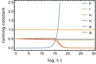
Figure 3: Running coupling constants at four dimensions. A prethermalization regime exists controlled by initial interaction values and the quench parameter $m$. After that, there is a new nonthermal fixed point.

Discussions.— To summarize, we explore nonequilibrium quantum electrodynamics following a global quench, revealing a noteworthy quantum memory effect in the form of a critical exponent, i.e., the fermion anomalous dimension. While our discussion is mainly focused on the 3+1 dimensional case, we conclude this paper by highlighting a few remaining open questions, including the 2+1 dimensional case. In equilibrium, quantum electrodynamics in 2+1 dimensions exhibits a nontrivial fixed point. We initiate an investigation of quench dynamics in 2+1 dimensions in the Appendix, where the quench trivializes the interacting fixed point, and the validity of the RG flow needs further investigation. Conducting a higher-order loop calculation and taking the large-N limit could provide valuable insights into the fate of the nonequilibrium fixed point in 2+1 dimensions. We leave such investigation to future work. Furthermore, it would be of immense significance to experimentally implement the quench protocol examined in this study. Potential experimental platforms include programmable cold atom systems and pump-probe experiments in condensed matter systems.

Acknowledgements.— The work of MRL is supported in part by the NSFC under Grant No. 11825404. MRL acknowledges the support from the Lavin-Bernick Grant during his visit to Tulane university. The work of SKJ is supported by a startup fund at Tulane University.

The Supplemental Materials for “Quantum electrodynamics under a quench”

.1 Propagators in Keldysh countour

Figure S1: A schematic contour of the quench dynamics. The vertical (horizontal) line denotes the imaginary-time (real-time Keldysh) evolution.

To study the quench dynamics of the Dirac fermion, we adopt the Keldysh contour as shown in Fig. S1, where the vertical line indicates the generation of the prequench state via imaginary time evolution. The dynamics of the system is determined by the action:

$$S_{E} =\int_{0}^{\beta}d\tau L_{E}\left[\bm{A},\psi_{i}^{\dagger},\psi_{i}\right],$$ (S1)

$$S_{R} =\int_{0}^{\infty}dt\left(L\left[\bm{A}_{+},\psi_{+}^{\dagger},\psi_{+}\right]-L\left[\bm{A}_{-},\psi_{-}^{\dagger},\psi_{-}\right]\right),$$

where ‘E’ and ‘R’ denote the Euclidean and real-time action separately. The Lagrangians are

$$L_{E}\left[\phi,\psi^{\dagger},\psi\right] = L_{E,b}[\phi]+L_{E,f}\left[\psi^{\dagger},\psi\right],$$ (S2)

$$L_{E,b}[\phi] = \frac{1}{4}\int_{x}F_{\mu\nu}F^{\mu\nu}=-\frac{1}{2}\int_{x}A_{\mu}\left(\partial^{2}g^{\mu\nu}-\partial^{\mu}\partial^{\nu}\right)A_{\nu}=\frac{1}{2}\int_{x}A_{\mu}k^{2}g^{\mu\nu}A_{\nu},$$ (S3)

$$L_{E,f}\left[\psi^{\dagger},\psi\right] = \int_{x}\psi^{\dagger}\left(\partial_{\tau}+H_{E}\right)\psi,$$ (S4)

$$L\left[\phi,\psi^{\dagger},\psi\right] = \int_{x}\left(\frac{1}{2}A_{\mu}k^{2}g^{\mu\nu}A_{\nu}+\psi^{\dagger}\left(i\partial_{t}-H_{R}\right)\psi+e\overline{\Psi}A_{\mu}\gamma^{\mu}\Psi\right),$$ (S5)

where the Hamiltonians of the fermion in imaginary-time and real-time are

$$H_{E}=\bm{k}\cdot\bm{\alpha}+m\gamma^{0},\quad H_{R}=\bm{k}\cdot\bm{\alpha}.$$ (S6)

The Dirac matrices satisfies $\{\gamma^{\mu},\gamma^{\nu}\}=2g^{\mu\nu}$ with the convention $g_{\mu\nu}=\text{diag}(1,-1,-1,-1)$. ${\bm{\alpha}}$ is defined via ${\bm{\alpha}}\equiv(\gamma^{0}\gamma^{1},\gamma^{0}\gamma^{2},\gamma^{0}\gamma^{3})$. Applying the Keldysh rotation

$$\psi_{c/q}=\frac{1}{\sqrt{2}}(\psi_{+}\pm\psi_{-}),\quad\psi_{c/q}^{\dagger}=\frac{1}{\sqrt{2}}(\psi_{+}^{\dagger}\mp\psi_{-}^{\dagger}),\quad A_{c/q}=\frac{1}{\sqrt{2}}(A_{+}\pm A_{-}),$$ (S7)

the real-time action is reduced to

$$S =S_{0}+S_{\text{int}},$$ (S8)

$$S_{0} =\int_{0}^{\infty}dt\int_{\bm{x}}\bar{\Psi}\left(\begin{array}[]{cccc}\mathfrak{i}\partial_{\mu}\gamma^{\mu}&0\\ 0&\mathfrak{i}\partial_{\mu}\gamma^{\mu}\end{array}\right)\Psi+\int_{0}^{\infty}dt\int_{\bm{x}}A_{c,q}\left(g^{\mu\nu}\partial^{2}-\partial^{\mu}\partial^{\nu}\right)A_{q,\nu},$$

$$S_{\text{int}} =\frac{1}{\sqrt{2}}\int_{0}^{\infty}dt\int_{\bm{x}}\left(e_{c}\bar{\Psi}A_{c,0}\gamma^{0}\Psi+g_{c}\bar{\Psi}A_{c,i}\gamma^{i}\Psi+e_{q}\bar{\Psi}A_{q,0}\rho^{x}\gamma^{0}\Psi+g_{q}\bar{\Psi}A_{q,i}\rho^{x}\gamma^{i}\Psi\right).$$

According to the Keldysh field theory, the propagators are given by

$$\hat{G} =-i\left\langle\Psi\Psi^{\dagger}\right\rangle=\left(\begin{array}[]{cc}G_{R}&G_{K}\\ 0&G_{A}\end{array}\right),\quad\hat{D} =-i\left\langle A_{\mu}A_{\nu}\right\rangle=\left(\begin{array}[]{cc}D_{K}&D_{R}\\ D_{A}&0\end{array}\right).$$ (S9)

in the classical/quantum fields basis. We introduce the source field $\xi_{c/q}$ that couples to the fermionic field $\psi_{c/q}$

$$W\left[\xi_{c/q}\right]=\ln\int D\mu_{f}\exp\left[-\int d\tau L_{E,f}\left[\psi_{i}^{\dagger},\psi_{i}\right]+i\int dt\left(L_{0,f}\left[\Psi^{\dagger},\Psi\right]+\left(\xi_{c}^{\dagger}\psi_{c}+\xi_{q}^{\dagger}\psi_{q}+H.c.\right)\right)\right],$$ (S10)

where $\int D\mu_{f}\equiv D\psi_{i}^{\dagger}D\psi_{i}D\psi_{c}^{\dagger}D\psi_{c}D\psi_{q}^{\dagger}D\psi_{q}$. By integrating the dynamical fields, one can get the fermion propagators. Integrating over $\psi_{i}^{\dagger}$, we can obtain the equation of motion of $\psi_{i}$: $(\partial_{\tau}+\mathcal{H})\psi_{i}=0$. The wave function can be solved directly. We assume the value of $\psi$ at time $\tau=0$ to be $\psi_{0}$, then the solution to the equation of motion is

$$\psi(\tau)=\left(e^{-\xi\tau}P_{+}(m)+e^{\xi\tau}P_{-}(m)\right)\psi_{0},$$ (S11)

where $P_{+/-}(m)$ are projectors that project to the positive/negative energy eigenstate:

$$P_{\pm}(m) =\frac{1}{2}\left(1\pm(\bm{\hat{k}}_{m}\cdot\bm{\alpha}+\hat{m}\gamma^{0})\right),$$ (S12)

$$H_{E}P_{\pm}(m) =\pm\xi P_{\pm}(m),\quad H_{R}P_{\pm}=\pm|\bm{k}|P_{\pm},$$

with $\xi=\sqrt{k^{2}+m^{2}}$. With the boundary condition $\psi_{-}(0)=-\psi_{i}(0),\psi_{+}(0)=\psi_{i}(\beta)$, the initial values of $\psi_{c/q}$ are given by

$$\psi_{c0} = \frac{1}{\sqrt{2}}(\psi(\beta)-\psi(0))=\frac{1}{\sqrt{2}}\left(\left(e^{-\xi\beta}P_{+}(m)+e^{\xi\beta}P_{-}(m)\right)-1\right)\psi_{0},$$ (S13)

$$\psi_{q0} = \frac{1}{\sqrt{2}}(\psi(\beta)+\psi(0))=\frac{1}{\sqrt{2}}\left(\left(e^{-\xi\beta}P_{+}(m)+e^{\xi\beta}P_{-}(m)\right)+1\right)\psi_{0},$$ (S14)

$$\psi_{c0}^{\dagger} = \frac{1}{\sqrt{2}}(\psi^{\dagger}(\beta)+\psi^{\dagger}(0))=\frac{1}{\sqrt{2}}\psi_{0}^{\dagger}\left(\left(e^{-\xi\beta}P_{+}(m)+e^{\xi\beta}P_{-}(m)\right)+1\right),$$ (S15)

$$\psi_{q0} = \frac{1}{\sqrt{2}}(\psi^{\dagger}(\beta)-\psi^{\dagger}(0))=\frac{1}{\sqrt{2}}\psi_{0}^{\dagger}\left(\left(e^{-\xi\beta}P_{+}(m)+e^{\xi\beta}P_{-}(m)\right)-1\right).$$ (S16)

After the integration of the fields $\psi_{i}$ and $\psi_{i}^{\dagger}$, the Eq. S10 is reduced to

$$W\left[\xi_{c/q}\right]=\ln\int D\psi_{0}D\psi_{c}^{\dagger}D\psi_{c}D\psi_{f}^{\dagger}D\psi_{f}\exp\left[i\int dt\left(\int_{\bm{x}}\bar{\Psi}\left(\begin{array}[]{cccc}\mathfrak{i}\partial_{\mu}\gamma^{\mu}&0\\ 0&\mathfrak{i}\partial_{\mu}\gamma^{\mu}\end{array}\right)\Psi+\left(\xi_{c}^{\dagger}\psi_{c}+\xi_{q}^{\dagger}\psi_{q}+\text{ H.c. }\right)\right)\right].$$ (S17)

Again we integrate $\psi_{c}^{\dagger}$ and $\psi_{q}$ and obtain the equation of motion of $\psi_{c}$ and $\psi_{q}^{\dagger}$:

$$\left(i\partial_{t}-\mathcal{H}\right)\psi_{c}+\xi_{c}=0,$$ (S18)

$$-i\partial_{t}\psi_{q}^{\dagger}-\psi_{q}^{\dagger}\mathcal{H}+\xi_{q}^{\dagger}=0.$$ (S19)

Using the boundary condition Eq. S13 and  S14, the solutions can be obtained directly

$$\psi_{c}(t) =\left[P_{+}\left(e^{-\xi\beta}P_{+}(m)+e^{\xi\beta}P_{-}(m)-1\right)e^{-ikt}+P_{-}\left(e^{-\xi\beta}P_{+}(m)+e^{\xi\beta}P_{-}(m)-1\right)e^{ikt}\right]\psi_{0}-\int dt^{\prime}G_{R}\left(\bm{k},t-t^{\prime}\right)\xi_{c}\left(t^{\prime}\right),$$ (S20)

$$\psi_{q}^{\dagger}(t) =\psi_{0}^{\dagger}\left[\left(e^{-\xi\beta}P_{+}(m)+e^{\xi\beta}P_{-}(m)-1\right)P_{+}e^{ikt}+\left(e^{-\xi\beta}P_{+}(m)+e^{\xi\beta}P_{-}(m)-1\right)P_{-}e^{-ikt}\right]-\int dt^{\prime}\xi_{q}^{\dagger}\left(t^{\prime}\right)G_{A}\left(\bm{k},t^{\prime}-t\right),$$

where $P_{\pm}\equiv P_{\pm}(0)$, and $G_{R/A}$ are the retarded and advanced Green’s function given by

$$G_{R}\left(\bm{k},t-t^{\prime}\right)=-i\Theta\left(t-t^{\prime}\right)\left(e^{-i|k|\left(t-t^{\prime}\right)}P_{+}(k)+e^{i|k|\left(t-t^{\prime}\right)}P_{-}(k)\right),$$ (S21)

$$G_{A}\left(\bm{k},t-t^{\prime}\right)=i\Theta\left(t^{\prime}-t\right)\left(e^{-i|k|\left(t-t^{\prime}\right)}P_{+}(k)+e^{i|k|\left(t-t^{\prime}\right)}P_{-}(k)\right).$$

Substituting the solution Eq. S20 into the action and integrating over $\psi_{c}$ and $\psi_{q}^{\dagger}$, we arrive at

$$e^{W\left[\xi_{c/q}\right]}= \exp-i\int dtdt^{\prime}\int_{k}\left[\xi_{c}^{\dagger}(t)G_{R}\left(k,t-t^{\prime}\right)\xi_{c}\left(t^{\prime}\right)+\xi_{q}^{\dagger}(t)G_{A}\left(k,t-t^{\prime}\right)\xi_{q}(t)\right]$$ (S22)

$$\times\int D\psi_{0}\exp\left(\psi_{0q}^{\dagger}\psi_{0q}\right)\exp\frac{i}{\sqrt{2}}\int dt\int_{k}\left[\xi_{c}^{\dagger}[P_{+}(e^{-\xi\beta}P_{+}(m)+e^{\xi\beta}P_{-}(m)-1\right)e^{-ikt}$$

$$+P_{-}\left(e^{-\xi\beta}P_{+}(m)+e^{\xi\beta}P_{-}(m)-1\right)e^{ikt}]\psi_{0}+$$

$$\psi_{0}^{\dagger}\left[\left(e^{-\xi\beta}P_{+}(m)+e^{\xi\beta}P_{-}(m)-1\right)P_{+}e^{ikt}+\left(e^{-\xi\beta}P_{+}(m)+e^{\xi\beta}P_{-}(m)-1\right)P_{-}e^{-ikt}\right]\xi_{q}].$$

Further integrating over $\psi_{0}$ leads to the generating function for free propagators:

$$W\left[\xi_{c/q}\right]=\int dtdt^{\prime}\int_{k}\left(-i\left[\xi_{c}^{\dagger}(t)G_{R}\left(k,t-t^{\prime}\right)\xi_{c}\left(t^{\prime}\right)+\xi_{q}^{\dagger}(t)G_{A}\left(k,t-t^{\prime}\right)\xi_{q}(t)\right]-\xi_{c}^{\dagger}(t)G_{K}(k,t-t^{\prime})\xi_{q}\left(t^{\prime}\right)\right),$$ (S23)

where

$$\mathfrak{i}G_{K}(t_{1},t_{2};\bm{k})=\tanh\frac{\beta\xi}{2}(e^{-\mathfrak{i}|\bm{k}|t_{1}}P_{+}+e^{\mathfrak{i}|\bm{k}|t_{1}}P_{-})(P_{+}(m)-P_{-}(m))(e^{\mathfrak{i}|\bm{k}|t_{2}}P_{+}+e^{-\mathfrak{i}|\bm{k}|t_{2}}P_{-}).$$ (S24)

Next, we turn to the boson propagator. The action of the free gauge boson is

$$L_{E,b}[\phi] = \frac{1}{4}\int_{x}F_{\mu\nu}F^{\mu\nu}=-\frac{1}{2}\int_{x}A_{\mu}\left(\partial^{2}g^{\mu\nu}-\partial^{\mu}\partial^{\nu}\right)A_{\nu}=\frac{1}{2}\int_{x}A_{\mu}k^{2}g^{\mu\nu}A_{\nu},$$ (S25)

The retarded Green’s function of the gauge field is given by

$$D_{\mu\nu}^{R}(\omega,\bm{k})=-g_{\mu\nu}\frac{1}{(\omega+i\delta-k)(\omega+i\delta+k)}=-g_{\mu\nu}\frac{1}{2k}\left(\frac{1}{\omega+i\delta-k}-\frac{1}{\omega+i\delta+k}\right).$$ (S26)

One can obtain the real-time retarded propagator by Fourier transformation

$$D_{\mu\nu}^{R}(t,\bm{k})=-g_{\mu\nu}\frac{1}{2k}\int\left(\frac{1}{\omega+i\delta-k}-\frac{1}{\omega+i\delta+k}\right)e^{-i\omega t}=-g_{\mu\nu}\theta[t]\left(-\frac{\operatorname{Sin}[kt]}{k}\right).$$ (S27)

The same calculation also follows for the advanced propagator

$$D_{\mu\nu}^{A}(\omega,\bm{k})=-g_{\mu\nu}\frac{1}{(\omega-i\delta-k)(\omega-i\delta+k)}=-g_{\mu\nu}\frac{1}{2k}\left(\frac{1}{\omega-i\delta-k}-\frac{1}{\omega-i\delta+k}\right)$$ (S28)

$$D_{\mu\nu}^{A}(t,\bm{k})=-g_{\mu\nu}\frac{1}{2k}\int\left(\frac{1}{\omega-i\delta-k}-\frac{1}{\omega-i\delta+k}\right)e^{-i\omega t}=-g_{\mu\nu}\theta[-t]\frac{\sin[kt]}{k}$$

Thus, we can write the time-ordered propagator

$$D_{\mu\nu}^{t}(t,\bm{k})=-g_{\mu\nu}\frac{-\mathfrak{i}}{2k}(\theta[t]e^{-\mathfrak{i}kt}+\theta[-t]e^{\mathfrak{i}kt}),$$ (S29)

and the two-point functions are

$$\left\langle A_{\mu}(t)A_{v}(0)\right\rangle=-g_{\mu v}\frac{e^{-ikt}}{2k},\left\langle A_{v}(0)A_{\mu}(t)\right\rangle=-g_{\mu v}\frac{e^{ikt}}{2k}.$$ (S30)

According to Eq. S9, the Keldysh propagator is

$$iD_{\mu v}^{K} =\left\langle A_{c}(t)A_{c}(0)\right\rangle=\frac{1}{2}\left\langle\left(A_{+}(t)+A_{-}(t)\right)\left(A_{+}(0)+A_{-}(0)\right)\right\rangle=\langle A(t)A(0)+A(0)A(t)\rangle-g_{\mu v}\frac{\operatorname{cos}[kt]}{k}.$$ (S31)

For later convenience, we modify the definition of the fermion propagators by attaching a $\gamma_{0}$ matrix to the original definition:

$$\hat{G} =-i\left\langle\Psi\overline{\Psi}\right\rangle=\left(\begin{array}[]{cc}G_{R}&G_{K}\\ 0&G_{A}\end{array}\right),$$ (S34)

with

$$G_{R}\left(\bm{k},t-t^{\prime}\right)=-i\Theta\left(t-t^{\prime}\right)\left(e^{-i|k|\left(t-t^{\prime}\right)}P_{+}(k)+e^{i|k|\left(t-t^{\prime}\right)}P_{-}(k)\right)\gamma^{0},$$ (S35)

$$G_{A}\left(\bm{k},t-t^{\prime}\right)=i\Theta\left(t^{\prime}-t\right)\left(e^{-i|k|\left(t-t^{\prime}\right)}P_{+}(k)+e^{i|k|\left(t-t^{\prime}\right)}P_{-}(k)\right)\gamma^{0},$$ (S36)

$$G_{K}(t_{1},t_{2};\bm{k})=-\mathfrak{i}\tanh\frac{\beta\xi}{2}(e^{-\mathfrak{i}|\bm{k}|t_{1}}P_{+}+e^{\mathfrak{i}|\bm{k}|t_{1}}P_{-})(P_{+}(m)-P_{-}(m))(e^{\mathfrak{i}|\bm{k}|t_{2}}P_{+}+e^{-\mathfrak{i}|\bm{k}|t_{2}}P_{-})\gamma^{0}.$$ (S37)

.2 Ward identity

In this section, we derive the Ward identity for the quenched fermion system. We start with the fermion action in equilibrium $S=\int\overline{\psi}\partial_{\mu}\gamma^{\mu}\psi$. The equilibrium fermion propagator is given by $G^{-1}=\mathfrak{i}\partial_{\mu}\gamma^{\mu}=k_{\mu}\gamma^{\mu}$, $G=\frac{k_{\mu}\gamma^{\mu}}{\bm{k}^{2}}$, within which the perturbative Ward identity can be derived:

$$G(\bm{k+p})-G(\bm{k}) =\frac{(k_{\mu}+p_{\mu})\gamma^{\mu}}{(\bm{k}+\bm{p})^{2}}-\frac{k_{\mu}\gamma^{\mu}}{\bm{k}^{2}}=\frac{\bm{k}^{2}(k_{\mu}+p_{\mu})\gamma^{\mu}-(\bm{k}+\bm{p})^{2}k_{\mu}\gamma^{\mu}}{(\bm{k}+\bm{p})^{2}\bm{k}^{2}}$$ (S38)

$$=\frac{\bm{k}^{2}p_{\mu}\gamma^{\mu}-2\bm{k}\cdot\bm{p}k_{\mu}\gamma^{\mu}-\bm{p}^{2}k_{\mu}\gamma^{\mu}}{(\bm{k}+\bm{p})^{2}\bm{k}^{2}}=-\frac{k_{\nu}\gamma^{\nu}p_{\mu}\gamma^{\mu}k_{\rho}\gamma^{\rho}+k_{\mu}\gamma^{\mu}p^{2}}{(\bm{k}+\bm{p})^{2}\bm{k}^{2}}$$

$$=-\frac{k_{\nu}\gamma^{\nu}p_{\mu}\gamma^{\mu}(k_{\rho}\gamma^{\rho}+p_{\rho}\gamma^{\rho})}{(\bm{k}+\bm{p})^{2}\bm{k}^{2}}=-p_{\mu}\frac{k_{\nu}\gamma^{\nu}}{\bm{k}^{2}}\gamma^{\mu}\frac{(k_{\rho}+p_{\rho})\gamma^{\rho}}{(\bm{k}+\bm{p})^{2}}$$

$$=-p_{\mu}G(\bm{k})\gamma^{\mu}G(\bm{k}+\bm{p}).$$

Thus, one can obtain the Ward identity in the frequency-momentum space $\partial^{\mu}G(\bm{k})=-G(\bm{k})\gamma^{\mu}G(\bm{k})$. However, in our case, the quench breaks the time translation symmetry explicitly, so we turn to the real-time coordinate

$$\int dt_{2}G(t_{1}-t_{2},\bm{k})\gamma^{\mu}G(t_{2}-t_{3},\bm{k}) =\int\frac{d\omega_{1}d\omega_{2}}{4\pi^{2}}\int dt_{2}\exp{[-\mathfrak{i}\omega_{1}(t_{1}-t_{2})-\mathfrak{i}\omega_{2}(t_{2}-t_{3})]}G(\omega_{1},\bm{k})\gamma^{\mu}G(\omega_{2},\bm{k})$$ (S39)

$$=\int\frac{d\omega}{2\pi}G(\omega,\bm{k})\gamma^{\mu}G(\omega,\bm{k})e^{-\mathfrak{i}\omega(t_{1}-t_{3})}=-\int\frac{d\omega}{2\pi}\partial_{k_{\mu}}G(\omega,\bm{k})e^{-\mathfrak{i}\omega(t_{1}-t_{3})}$$

$$=-\partial_{k_{\mu}}G(t_{1}-t_{3},\bm{k}).$$

In particular, we can write the above equation in another form

$$G(t_{1},t_{3};\bm{k}+\bm{p})-G(t_{1},t_{3};\bm{k})=-\int dt_{2}\left[cp_{i}G(t_{1},t_{2};\bm{k})\gamma^{i}G(t_{2},t_{3};\bm{k}+\bm{p})+\mathfrak{i}\partial_{t_{2}}G(t_{1},t_{2};\bm{k})\gamma^{0}G(t_{2},t_{3};\bm{k}+\bm{p})\right].$$ (S40)

where the second term of the r.h.s is the surface term and will disappear in equilibrium.

.3 RG analysis

In this section, we give a brief derivation of the RG equations. As derived in the main text, the Keldysh action for the fermion coupled to gauge boson is given by

$$S =S_{0}+S_{\text{int}},$$ (S41)

$$S_{0} =\int_{0}^{\infty}dt\int_{\bm{x}}\bar{\Psi}\left(\begin{array}[]{cccc}\mathfrak{i}\partial_{\mu}\gamma^{\mu}&0\\ 0&\mathfrak{i}\partial_{\mu}\gamma^{\mu}\end{array}\right)\Psi+\int_{0}^{\infty}dt\int_{\bm{x}}A_{c,q}\left(g^{\mu\nu}\partial^{2}-\partial^{\mu}\partial^{\nu}\right)A_{q,\nu},$$

$$S_{\text{int}} =\frac{1}{\sqrt{2}}\int_{0}^{\infty}dt\int_{\bm{x}}\left(e_{c}\bar{\Psi}A_{c,0}\gamma^{0}\Psi+g_{c}\bar{\Psi}A_{c,i}\gamma^{i}\Psi+e_{q}\bar{\Psi}A_{q,0}\rho^{x}\gamma^{0}\Psi+g_{q}\bar{\Psi}A_{q,i}\rho^{x}\gamma^{i}\Psi\right).$$

Figure S2: The Feynman diagrams that correct bosonic and fermionic two-point correlations.

We then treat the interaction terms $S_{\text{int}}$ as a perturbation. The second-order perturbation gives the correction to the two-point correlations. The corresponding Feynman diagrams are shown in Fig. S2. (a), (b), and (c) of Fig. S2 are the corrections to the two-point fermion correlator:

(a)+(b)+(c) $$=\frac{i}{2}\frac{e_{c}e_{q}}{2}\int\bar{\psi}(t_{1})\left\langle\rho^{x}\gamma^{\mu}\psi(t_{1})\bar{\psi}(t_{2})\gamma^{\nu}A_{q,\mu}(t_{1})A_{c,\nu}(t_{2})\right\rangle\psi(t_{2})$$ (S42)

$$+\frac{i}{2}\frac{e_{c}e_{q}}{2}\int\bar{\psi}(t_{1})\left\langle\gamma^{\mu}\psi(t_{1})\bar{\psi}(t_{2})\rho^{x}\gamma^{\nu}A_{c,\mu}(t_{1})A_{q,v}(t_{2})\right\rangle\psi(t_{2})$$

$$+\frac{i}{2}\frac{e_{c}^{2}}{2}\int\bar{\psi}(t_{1})\left\langle\gamma^{\mu}\psi(t_{1})\bar{\psi}(t_{2})\gamma^{\nu}A_{c,\mu}(t_{1})A_{c,v}(t_{2})\right\rangle\psi(t_{2})$$

$$=\frac{i}{2}\frac{e_{c}e_{q}}{2}\int\bar{\psi}(t_{1})\frac{1}{4}\operatorname{Tr}\left[\gamma^{\mu}(iG(t_{1},t_{2}))\rho^{x}\gamma^{\nu}\right]\left(\dot{i}D_{\mu\nu}^{R}(t_{1},t_{2})\right)\psi(t_{2})$$

$$+\frac{i}{2}\frac{e_{c}e_{q}}{2}\int\bar{\psi}(t_{1})\frac{1}{4}\operatorname{Tr}\left[\rho^{x}\gamma^{\mu}(\dot{i}G(t_{1},t_{2}))\gamma^{\nu}\right]\left(iD_{\nu\mu}^{R}(t_{2},t_{1})\right)\psi(t_{2})$$

$$+\frac{i}{2}e_{c}^{2}\int\bar{\psi}(t_{1})\gamma^{\alpha}\psi(t_{2})\frac{1}{4}\operatorname{Tr}\left[\gamma_{\alpha}\gamma^{\mu}(iG(t_{1},t_{2}))\gamma^{\nu}\right]\left(iD_{\nu\mu}^{K}(t_{2},t_{1})\right).$$

Substituting the exact forms of the propagators into the Eq. S42, one can obtain

(a)+(b)+(c) $$=i\int\bar{\Psi}\left(\frac{(3g_{c}g_{q}-e_{c}e_{q})}{32c^{3}\sqrt{k^{2}+m^{2}}\pi^{2}}\gamma^{0}\partial_{t}+\frac{\left(3g_{c}^{2}-e_{c}^{2}\right)}{32c^{3}k\pi^{2}}\gamma^{0}\partial_{t}\right)\Psi$$ (S43)

$$+i\int\bar{\Psi}\left(\frac{(e_{c}e_{q}+g_{c}g_{q})\left(3k^{2}+5m^{2}\right)}{96c^{3}\left(k^{2}+m^{2}\right)^{3/2}\pi^{2}}c\gamma^{i}\partial_{i}+\frac{\left(e_{c}^{2}+g_{c}^{2}\right)}{32c^{3}k\pi^{2}}c\gamma^{i}\partial_{i}\right)\Psi.$$

The light velocity $c$ is renormalized by:

$$\frac{dc}{dl}=\left(\frac{(e_{c}e_{q}+g_{c}g_{q})\left(3+5\Omega^{2}\right)}{96\pi^{2}c^{3}\left(1+\Omega^{2}\right)^{3/2}}-\frac{3g_{c}g_{q}-e_{c}e_{q}}{32\pi^{2}c^{3}\sqrt{1+\Omega^{2}}}+\frac{e_{c}^{2}-g_{c}^{2}}{16c^{3}\pi^{2}}\right)c,$$ (S44)

where $\Lambda$ is the energy cutoff and $\Omega\equiv\frac{m}{\Lambda}$ is the quench parameter. Then the fermionic anomalous dimension is $\eta_{f}=\frac{3g_{c}g_{q}-e_{c}e_{q}}{32\pi^{2}c^{3}\sqrt{1+\Omega^{2}}}+\frac{3g_{c}^{2}-e_{c}^{2}}{32\pi^{2}c^{3}}$.

In the same way, one can calculate the diagrams (d) and (e) in Fig. S2 and obtain the 2-point corrections to the gauge boson:

$$(d)+(e) =\frac{i}{2}\left\langle\left(\frac{e_{c}}{\sqrt{2}}\int A_{c,\mu}\bar{\psi}\gamma^{\mu}\psi+\frac{e_{q}}{\sqrt{2}}\int A_{q,\mu}\bar{\psi}\rho^{x}\gamma^{\mu}\psi\right)^{2}\right\rangle$$ (S45)

$$=\frac{i}{2}e_{c}e_{q}\int A_{q,\mu}A_{c,\nu}\left\langle\bar{\psi}\rho^{x}\gamma^{\mu}\psi\bar{\psi}\gamma^{v}\psi\right\rangle$$

$$=-\frac{i}{2}e_{c}e_{q}\int A_{q,\mu}(t_{1})A_{c,\nu}(t_{2})\operatorname{Tr}\left[\rho^{x}\gamma^{\mu}iG(t_{1},t_{2})\gamma^{v}iG(t_{2},t_{1})\right].$$

With the quenched propagators, the Eq. S45 can be calculated:

$$\frac{i}{2}\left\langle s_{\text{int }}^{2}\right\rangle =\int A_{q,0}\left(-c^{2}\nabla^{2}\right)A_{c,0}\int dk\frac{e_{c}e_{q}}{6\pi^{2}c^{3}\left(k^{2}+m^{2}\right)^{1/2}}$$ (S46)

$$+\int A_{q,y}\left(\partial_{t}^{2}-c^{2}\left(\partial_{x}^{2}+\partial_{z}^{2}\right)\right)A_{c,y}\int dk\frac{g_{c}g_{q}}{6\pi^{2}c^{3}\left(k^{2}+m^{2}\right)^{1/2}}$$

$$+\int A_{q,y}c^{2}\nabla^{2}A_{c,y}\int dk\frac{\left(m^{4}-2k^{2}m^{2}\right)g_{c}g_{q}}{15\pi^{2}c^{3}\left(k^{2}+m^{2}\right)^{5/2}}\ldots$$

The last term can be ignored, then the Eq. S46 gives the boson’s anomalous dimension $\eta_{b_{t}}=\frac{e_{c}e_{q}}{6\pi^{2}c^{3}(1+\Omega^{2})^{1/2}}$, $\eta_{b_{x/y/z}}=\frac{g_{c}g_{q}}{6\pi^{2}c^{3}(1+\Omega^{2})^{1/2}}$.

Figure S3: The Feynman diagrams that correct the interactions.

To renormalize the interacting terms $g_{c/q},e_{c/q}$, one needs to calculate the third-order perturbation of the interactions. The corresponding Feynman diagrams are shown in Fig. S3, and the correction $\delta S_{v}$ is given by

$$\delta S_{v} =\int_{0}^{\infty}dt\int\left(\frac{7(e_{c}e_{q}+g_{c}g_{q})}{48\pi^{2}c^{3}\sqrt{1+\Omega^{2}}}+\frac{e_{c}^{2}+g_{c}^{2}}{16\pi^{2}c^{3}}\right)\log\Lambda\left(\frac{g_{c}}{2\sqrt{2}}\bar{\Psi}A_{c,i}\gamma^{i}\Psi\right).$$ (S47)

$$+\int_{0}^{\infty}dt\int\left(\frac{7(e_{c}e_{q}+g_{c}g_{q})}{48\pi^{2}c^{3}\sqrt{1+\Omega^{2}}}+\frac{(e_{c}^{2}+g_{c}^{2})(5+\Omega^{2})}{48\pi^{2}c^{3}(1+\Omega^{2})}\right)\log\Lambda\left(\frac{g_{q}}{2\sqrt{2}}\bar{\Psi}A_{q,i}\rho^{x}\gamma^{i}\Psi\right).$$

Notice that the results of the time component $e_{c}$ and $e_{q}$ are direct, but one needs to pay additional attention to the space case. According to the Ward identity Eq. S40, the vertex contribution of the interacting term differs from the fermionic contribution by a surface contribution.

With the results obtained above, the flow equations for the interactions can then be derived directly

$$\frac{de_{c}}{dl}=\left(\frac{\epsilon}{2}-\frac{\eta_{bt}}{2}-\eta_{f}\right)e_{c}+\left(\frac{3g_{c}g_{q}-e_{c}e_{q}}{32\pi^{2}c^{3}\sqrt{1+\Omega^{2}}}+\frac{3g_{c}^{2}-e_{c}^{2}}{32\pi^{2}c^{3}}\right)e_{c},$$ (S48)

$$\frac{dg_{c}}{dl}=\left(\frac{\epsilon}{2}-\frac{\eta_{bxyz}}{2}-\eta_{f}\right)g_{c}+\left(\frac{7(e_{c}e_{q}+g_{c}g_{q})}{96\pi^{2}c^{3}\sqrt{1+\Omega^{2}}}+\frac{e_{c}^{2}+g_{c}^{2}}{32\pi^{2}c^{3}}\right)g_{c},$$

$$\frac{de_{q}}{dl}=\left(\frac{\epsilon}{2}-\frac{\eta_{bt}}{2}-\eta_{f}\right)e_{c}+\left(\frac{3g_{c}g_{q}-e_{c}e_{q}}{32\pi^{2}c^{3}\sqrt{1+\Omega^{2}}}+\frac{3g_{c}^{2}-e_{c}^{2}}{32\pi^{2}c^{3}}\right)e_{q},$$

$$\frac{dg_{q}}{dl}=\left(\frac{\epsilon}{2}-\frac{\eta_{bxyz}}{2}-\eta_{f}\right)g_{c}+\left(\frac{7(e_{c}e_{q}+g_{c}g_{q})}{96\pi^{2}c^{3}\sqrt{1+\Omega^{2}}}+\frac{(e_{c}^{2}+g_{c}^{2})(5+\Omega^{2})}{48\pi^{2}c^{3}(1+\Omega^{2})}\right)g_{c}.$$

To make the RG equations easier to manipulate and get a more direct understanding of the RG flow, one can define

$$e_{1}=e_{c}^{2}\Lambda^{-\epsilon},\quad e_{2}=\frac{e_{c}e_{q}}{\sqrt{1+\Omega^{2}}}\Lambda^{-\epsilon},$$ (S49)

$$g_{1}=g_{c}^{2}\Lambda^{-\epsilon},\quad g_{2}=\frac{g_{c}g_{q}}{\sqrt{1+\Omega^{2}}}\Lambda^{-\epsilon},$$ (S50)

and substitute into Eq. S48, then the RG equations reduce to

$$\frac{d\Omega}{dl} = \Omega,$$ (S51)

$$\frac{dc}{dl} = \frac{e_{1}-g_{1}+e_{2}-g_{2}}{16\pi^{2}c^{3}}+\frac{(e_{2}+g_{2})\Omega^{2}}{48\pi^{2}c^{3}(1+\Omega^{2})},$$ (S52)

$$\frac{de_{1}}{dl} = \left(\epsilon-\frac{e_{2}}{6\pi^{2}c^{3}}\right)e_{1},$$ (S53)

$$\frac{de_{2}}{dl} = \left(\epsilon-\frac{\Omega^{2}}{1+\Omega^{2}}-\frac{e_{2}}{6\pi^{2}c^{3}}\right)e_{2},$$ (S54)

$$\frac{dg_{1}}{dl} = \left(\epsilon+\frac{3(e_{1}-g_{1})+5(e_{2}-g_{2})}{24\pi^{2}c^{3}}\right)g_{1},$$ (S55)

$$\frac{dg_{2}}{dl} = \left(\epsilon-\frac{\Omega^{2}}{1+\Omega^{2}}+\frac{11e_{1}+20e_{2}-13g_{1}-20g_{2}+8(e_{1}+g_{1})/(1+\Omega^{2})}{96\pi^{2}c^{3}}\right)g_{2}.$$ (S56)

This leads to the RG equation in the main text.

We are ready to evaluate the non-trivial fixed point presented in the main text. Assuming a constant light velocity $c$, and notice that Eq. S51, Eq. S53 and Eq. S54 are decoupled from the rest equations, and one can obtain their solutions for $\epsilon=0$

$$\Omega(l) = \Omega_{0}e^{l},$$ (S57)

$$e_{1}(l) = \frac{e_{1}(0)}{1+e_{2}(0)\frac{\sqrt{1+\Omega_{0}^{2}}}{12\pi^{2}c^{3}}\log\left(\frac{\sqrt{1+\Omega_{0}^{2}}+1}{\sqrt{1+\Omega_{0}^{2}}-1}\frac{\sqrt{1+\Omega_{0}^{2}e^{2l}}-1}{\sqrt{1+\Omega_{0}^{2}e^{2l}}+1}\right)},$$ (S58)

$$e_{2}(l) = \frac{\left(\frac{1+\Omega_{0}^{2}}{1+\Omega_{0}^{2}e^{2l}}\right)^{1/2}e_{2}(0)}{1+e_{2}(0)\frac{\sqrt{1+\Omega_{0}^{2}}}{12\pi^{2}c^{3}}\log\left(\frac{\sqrt{1+\Omega_{0}^{2}}+1}{\sqrt{1+\Omega_{0}^{2}}-1}\frac{\sqrt{1+\Omega_{0}^{2}e^{2l}}-1}{\sqrt{1+\Omega_{0}^{2}e^{2l}}+1}\right)}.$$ (S59)

Take $l$ tends to infinity, $e_{1}$ and $e_{2}$ reaches the fixed point

$$e_{1}^{\ast}=\frac{e_{1}(0)}{1+e_{2}(0)\frac{\sqrt{1+\Omega_{0}^{2}}}{12\pi^{2}c^{3}}\log\left(\frac{\sqrt{1+\Omega_{0}^{2}}+1}{\sqrt{1+\Omega_{0}^{2}}-1}\right)},\quad e_{2}^{\ast}=0.$$ (S60)

Further, we can plug the fixed point solution into the RG equation for $g_{1}$ and $g_{2}$ to obtain

$$\frac{dg_{1}}{dl} = \left(\frac{3(e_{1}^{\ast}-g_{1})-5g_{2}}{24\pi^{2}c^{3}}\right)g_{1},$$ (S61)

$$\frac{dg_{2}}{dl} = \left(-1+\frac{11e_{1}-13g_{1}-20g_{2}}{96\pi^{2}c^{3}}\right)g_{2}.$$ (S62)

The $g_{2}$ is already irrelevant at the tree level, it goes to zero $g_{2}^{\ast}=0$ at low energies. On the other hand, $g_{1}$ satisfies the RG equation $\frac{dg_{1}}{dl}=\frac{3(e_{1}^{\ast}-g_{1})}{24\pi^{2}c^{3}}g_{1}$, so it goes to $g_{1}^{\ast}=e_{1}^{\ast}$. Within the fixed point obtained at the long-time limit, one can check the renormalization of the light velocity $c$ and find that $\frac{dc}{dl}=0$, consistent with our previous assumption.

.4 d=2+1

We present our preliminary investigation for the 2+1 dimension case. QED in 2+1 dimension ($\text{QED}_{3}$) is particularly interesting for its unique features compared to $\text{QED}_{4}$, such as confinement, chiral symmetry breaking, and dynamical mass generation [85, 86, 87, 88, 89]. It has been interpreted as an effective theory to describe various exotic physical phenomena like high-temperature superconductors [72, 73]. To get an insight into the quenched QED in 2+1 dimension, we first solve the fixed point. Again, we assume a constant light velocity $c$, and one can solve the RG equations for $d=3$ and obtain two nonthermal fixed points solutions: $e_{1}=e_{2}=g_{1}=g_{2}=0$ and $e_{2}=6c^{3}\pi^{2},e_{1}=-g_{1},g_{2}=\frac{6}{5}(e_{1}+9c^{3}\pi^{2})$. Only the trivial fixed point is stable for the initial physical isotropic interaction value $e_{1}=e_{2}=g_{1}=g_{2}$. The numerical results show that in the prethermal region the velocity $c$ flows to zero, while the Dirac fermion decouples from the gauge field with $e_{1;2}=g_{1;2}=0$. However, before the decoupling, the interaction terms flow to large finite values which is beyond the perturbation condition. On a long timescale $\Lambda t>\frac{1}{\Omega_{0}}$, since $c$ remains zero, the non-thermal fixed point is still trivial, while the equilibrium fixed point in $d=2+1$ should be finite. Thus, one can conclude that the quench will trivialize the quantum electrodynamics of the Dirac fermion in 2+1 dimension. Though all the interaction terms and the light velocity $c$ at the fixed point are zero, the fermion anomalous dimension at the nonthermal fixed point is zero. Note that, in contrast to the equilibrium $\text{QED}_{3}$, the fermion mass here is generated by the initial quench rather than the interactions, which distinguishes the postthermal behaviors from the regular $\text{QED}_{3}$. Considering higher-order corrections and taking the large-N limit may provide more insight into the 2+1d quenched QED.

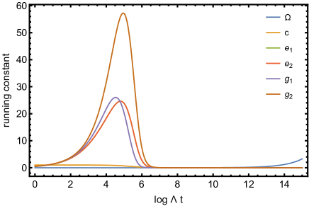
Figure S4: Running coupling constants in three dimensions. There exists a prethermalization regime where interactions increase and seem to be relevant as the regular QED behavior in 2+1 dimension. On the long timescale, the light velocity flows to zero and there is a new nonthermal fixed point that is trivial $g_{1}=g_{2}=e_{1}=e_{2}=0$.

References

• Polkovnikov et al. [2011] A. Polkovnikov, K. Sengupta, A. Silva, and M. Vengalattore, Colloquium: Nonequilibrium dynamics of closed interacting quantum systems, Rev. Mod. Phys. 83, 863 (2011).
• Blatt and Roos [2012] R. Blatt and C. F. Roos, Quantum simulations with trapped ions, Nature Physics 8, 277 (2012).
• Pogorelov et al. [2021] I. Pogorelov, T. Feldker, C. D. Marciniak, L. Postler, G. Jacob, O. Krieglsteiner, V. Podlesnic, M. Meth, V. Negnevitsky, M. Stadler, B. Höfer, C. Wächter, K. Lakhmanskiy, R. Blatt, P. Schindler, and T. Monz, Compact ion-trap quantum computing demonstrator, PRX Quantum 2, 020343 (2021).
• Bernien et al. [2017] H. Bernien, S. Schwartz, A. Keesling, H. Levine, A. Omran, H. Pichler, S. Choi, A. S. Zibrov, M. Endres, M. Greiner, V. Vuletić, and M. D. Lukin, Probing many-body dynamics on a 51-atom quantum simulator, Nature 551, 579 (2017).
• Ebadi et al. [2021] S. Ebadi, T. T. Wang, H. Levine, A. Keesling, G. Semeghini, A. Omran, D. Bluvstein, R. Samajdar, H. Pichler, W. W. Ho, S. Choi, S. Sachdev, M. Greiner, V. Vuletić, and M. D. Lukin, Quantum phases of matter on a 256-atom programmable quantum simulator, Nature 595, 227 (2021).
• Noel et al. [2022] C. Noel, P. Niroula, D. Zhu, A. Risinger, L. Egan, D. Biswas, M. Cetina, A. V. Gorshkov, M. J. Gullans, D. A. Huse, and C. Monroe, Measurement-induced quantum phases realized in a trapped-ion quantum computer, Nature Physics 18, 760 (2022).
• Chertkov et al. [2023] E. Chertkov, Z. Cheng, A. C. Potter, S. Gopalakrishnan, T. M. Gatterman, J. A. Gerber, K. Gilmore, D. Gresh, A. Hall, A. Hankin, M. Matheny, T. Mengle, D. Hayes, B. Neyenhuis, R. Stutz, and M. Foss-Feig, Characterizing a non-equilibrium phase transition on a quantum computer, Nature Physics 10.1038/s41567-023-02199-w (2023).
• Carollo et al. [2020] F. Carollo, F. M. Gambetta, K. Brandner, J. P. Garrahan, and I. Lesanovsky, Nonequilibrium quantum many-body rydberg atom engine, Phys. Rev. Lett. 124, 170602 (2020).
• Bluvstein et al. [2021] D. Bluvstein, A. Omran, H. Levine, A. Keesling, G. Semeghini, S. Ebadi, T. T. Wang, A. A. Michailidis, N. Maskara, W. W. Ho, S. Choi, M. Serbyn, M. Greiner, V. Vuletić, and M. D. Lukin, Controlling quantum many-body dynamics in driven rydberg atom arrays, Science 371, 1355 (2021)https://www.science.org/doi/pdf/10.1126/science.abg2530 .
• Nill et al. [2022] C. Nill, K. Brandner, B. Olmos, F. Carollo, and I. Lesanovsky, Many-body radiative decay in strongly interacting rydberg ensembles, Phys. Rev. Lett. 129, 243202 (2022).
• Smallwood et al. [2012] C. L. Smallwood, J. P. Hinton, C. Jozwiak, W. Zhang, J. D. Koralek, H. Eisaki, D.-H. Lee, J. Orenstein, and A. Lanzara, Tracking cooper pairs in a cuprate superconductor by ultrafast angle-resolved photoemission, Science 336, 1137 (2012)https://www.science.org/doi/pdf/10.1126/science.1217423 .
• Mankowsky et al. [2014] R. Mankowsky, A. Subedi, M. Först, S. O. Mariager, M. Chollet, H. T. Lemke, J. S. Robinson, J. M. Glownia, M. P. Minitti, A. Frano, M. Fechner, N. A. Spaldin, T. Loew, B. Keimer, A. Georges, and A. Cavalleri, Nonlinear lattice dynamics as a basis for enhanced superconductivity in yba2cu3o6.5, Nature 516, 71 (2014).
• Eisert et al. [2015] J. Eisert, M. Friesdorf, and C. Gogolin, Quantum many-body systems out of equilibrium, Nature Physics 11, 124 (2015).
• Srednicki [1994] M. Srednicki, Chaos and quantum thermalization, Phys. Rev. E 50, 888 (1994).
• Deutsch [1991] J. M. Deutsch, Quantum statistical mechanics in a closed system, Phys. Rev. A 43, 2046 (1991).
• Rigol et al. [2008] M. Rigol, V. Dunjko, and M. Olshanii, Thermalization and its mechanism for generic isolated quantum systems, Nature 452, 854 (2008).
• Berges et al. [2004] J. Berges, S. Borsányi, and C. Wetterich, Prethermalization, Phys. Rev. Lett. 93, 142002 (2004).
• Gring et al. [2012] M. Gring, M. Kuhnert, T. Langen, T. Kitagawa, B. Rauer, M. Schreitl, I. Mazets, D. A. Smith, E. Demler, and J. Schmiedmayer, Relaxation and prethermalization in an isolated quantum system, Science 337, 1318 (2012)https://www.science.org/doi/pdf/10.1126/science.1224953 .
• Langen et al. [2016] T. Langen, T. Gasenzer, and J. Schmiedmayer, Prethermalization and universal dynamics in near-integrable quantum systems, Journal of Statistical Mechanics: Theory and Experiment 2016, 064009 (2016).
• Langen et al. [2013] T. Langen, R. Geiger, M. Kuhnert, B. Rauer, and J. Schmiedmayer, Local emergence of thermal correlations in an isolated quantum many-body system, Nature Physics 9, 640 (2013).
• Eigen et al. [2018] C. Eigen, J. A. P. Glidden, R. Lopes, E. A. Cornell, R. P. Smith, and Z. Hadzibabic, Universal prethermal dynamics of bose gases quenched to unitarity, Nature 563, 221 (2018).
• Mitra [2018] A. Mitra, Quantum quench dynamics, Annual Review of Condensed Matter Physics 9, 245 (2018)https://doi.org/10.1146/annurev-conmatphys-031016-025451 .
• Mori et al. [2018] T. Mori, T. N. Ikeda, E. Kaminishi, and M. Ueda, Thermalization and prethermalization in isolated quantum systems: a theoretical overview, Journal of Physics B: Atomic, Molecular and Optical Physics 51, 112001 (2018).
• Jian et al. [2019] S.-K. Jian, S. Yin, and B. Swingle, Universal prethermal dynamics in gross-neveu-yukawa criticality, Phys. Rev. Lett. 123, 170606 (2019).
• Yin and Jian [2021] S. Yin and S.-K. Jian, Fermion-induced dynamical critical point, Phys. Rev. B 103, 125116 (2021).
• Shu et al. [2022] Y.-R. Shu, S.-K. Jian, and S. Yin, Nonequilibrium dynamics of deconfined quantum critical point in imaginary time, Phys. Rev. Lett. 128, 020601 (2022).
• Kyprianidis et al. [2021] A. Kyprianidis, F. Machado, W. Morong, P. Becker, K. S. Collins, D. V. Else, L. Feng, P. W. Hess, C. Nayak, G. Pagano, N. Y. Yao, and C. Monroe, Observation of a prethermal discrete time crystal, Science 372, 1192 (2021)https://www.science.org/doi/pdf/10.1126/science.abg8102 .
• Vu and Das Sarma [2023] D. Vu and S. Das Sarma, Dissipative prethermal discrete time crystal, Phys. Rev. Lett. 130, 130401 (2023).
• Kao et al. [2021] W. Kao, K.-Y. Li, K.-Y. Lin, S. Gopalakrishnan, and B. L. Lev, Topological pumping of a 1d dipolar gas into strongly correlated prethermal states, Science 371, 296 (2021)https://www.science.org/doi/pdf/10.1126/science.abb4928 .
• Shu et al. [2023] Y.-R. Shu, S.-K. Jian, A. W. Sandvik, and S. Yin, Equilibration of topological defects at the deconfined quantum critical point, arXiv preprint arXiv:2305.04771  (2023).
• Calabrese and Gambassi [2005] P. Calabrese and A. Gambassi, Ageing properties of critical systems, Journal of Physics A: Mathematical and General 38, R133 (2005).
• Täuber [2014] U. Täuber, A field theory approach to equilibrium and non-equilibrium scaling behavior (2014).
• Kollar et al. [2011] M. Kollar, F. A. Wolf, and M. Eckstein, Generalized gibbs ensemble prediction of prethermalization plateaus and their relation to nonthermal steady states in integrable systems, Phys. Rev. B 84, 054304 (2011).
• Van den Worm et al. [2013] M. Van den Worm, B. C. Sawyer, J. J. Bollinger, and M. Kastner, Relaxation timescales and decay of correlations in a long-range interacting quantum simulator, New Journal of Physics 15, 083007 (2013).
• Marcuzzi et al. [2013] M. Marcuzzi, J. Marino, A. Gambassi, and A. Silva, Prethermalization in a nonintegrable quantum spin chain after a quench, Phys. Rev. Lett. 111, 197203 (2013).
• Smith et al. [2013] D. A. Smith, M. Gring, T. Langen, M. Kuhnert, B. Rauer, R. Geiger, T. Kitagawa, I. Mazets, E. Demler, and J. Schmiedmayer, Prethermalization revealed by the relaxation dynamics of full distribution functions, New Journal of Physics 15, 075011 (2013).
• Bertini et al. [2015] B. Bertini, F. H. L. Essler, S. Groha, and N. J. Robinson, Prethermalization and thermalization in models with weak integrability breaking, Phys. Rev. Lett. 115, 180601 (2015).
• Buchhold et al. [2016] M. Buchhold, M. Heyl, and S. Diehl, Prethermalization and thermalization of a quenched interacting luttinger liquid, Phys. Rev. A 94, 013601 (2016).
• Mark et al. [2020] D. K. Mark, C.-J. Lin, and O. I. Motrunich, Exact eigenstates in the lesanovsky model, proximity to integrability and the pxp model, and approximate scar states, Phys. Rev. B 101, 094308 (2020).
• Berges et al. [2008] J. Berges, A. Rothkopf, and J. Schmidt, Nonthermal fixed points: Effective weak coupling for strongly correlated systems far from equilibrium, Phys. Rev. Lett. 101, 041603 (2008).
• Nowak et al. [2011] B. Nowak, D. Sexty, and T. Gasenzer, Superfluid turbulence: Nonthermal fixed point in an ultracold bose gas, Phys. Rev. B 84, 020506 (2011).
• Schole et al. [2012] J. Schole, B. Nowak, and T. Gasenzer, Critical dynamics of a two-dimensional superfluid near a nonthermal fixed point, Phys. Rev. A 86, 013624 (2012).
• Berges et al. [2014] J. Berges, K. Boguslavski, S. Schlichting, and R. Venugopalan, Turbulent thermalization process in heavy-ion collisions at ultrarelativistic energies, Phys. Rev. D 89, 074011 (2014).
• Piñeiro Orioli et al. [2015] A. Piñeiro Orioli, K. Boguslavski, and J. Berges, Universal self-similar dynamics of relativistic and nonrelativistic field theories near nonthermal fixed points, Phys. Rev. D 92, 025041 (2015).
• Erne et al. [2018] S. Erne, R. Bücker, T. Gasenzer, J. Berges, and J. Schmiedmayer, Universal dynamics in an isolated one-dimensional bose gas far from equilibrium, Nature 563, 225 (2018).
• Prüfer et al. [2018] M. Prüfer, P. Kunkel, H. Strobel, S. Lannig, D. Linnemann, C.-M. Schmied, J. Berges, T. Gasenzer, and M. K. Oberthaler, Observation of universal dynamics in a spinor bose gas far from equilibrium, Nature 563, 217 (2018).
• Schmied et al. [2019] C.-M. Schmied, A. N. Mikheev, and T. Gasenzer, Prescaling in a far-from-equilibrium bose gas, Phys. Rev. Lett. 122, 170404 (2019).
• Fujimoto et al. [2019] K. Fujimoto, R. Hamazaki, and M. Ueda, Flemish strings of magnetic solitons and a nonthermal fixed point in a one-dimensional antiferromagnetic spin-1 bose gas, Phys. Rev. Lett. 122, 173001 (2019).
• Mazeliauskas and Berges [2019] A. Mazeliauskas and J. Berges, Prescaling and far-from-equilibrium hydrodynamics in the quark-gluon plasma, Phys. Rev. Lett. 122, 122301 (2019).
• Bhattacharyya et al. [2020] S. Bhattacharyya, J. F. Rodriguez-Nieva, and E. Demler, Universal prethermal dynamics in heisenberg ferromagnets, Phys. Rev. Lett. 125, 230601 (2020).
• Claassen [2021] M. Claassen, Flow renormalization and emergent prethermal regimes of periodically-driven quantum systems (2021), arXiv:2103.07485 [quant-ph] .
• Marino et al. [2022] J. Marino, M. Eckstein, M. S. Foster, and A. M. Rey, Dynamical phase transitions in the collisionless pre-thermal states of isolated quantum systems: theory and experiments, Reports on Progress in Physics 85, 116001 (2022).
• Calabrese and Cardy [2006] P. Calabrese and J. Cardy, Time dependence of correlation functions following a quantum quench, Phys. Rev. Lett. 96, 136801 (2006).
• Calabrese and Cardy [2007] P. Calabrese and J. Cardy, Quantum quenches in extended systems, Journal of Statistical Mechanics: Theory and Experiment 2007, P06008 (2007).
• Eckstein et al. [2009] M. Eckstein, M. Kollar, and P. Werner, Thermalization after an interaction quench in the hubbard model, Phys. Rev. Lett. 103, 056403 (2009).
• Sciolla and Biroli [2010] B. Sciolla and G. Biroli, Quantum quenches and off-equilibrium dynamical transition in the infinite-dimensional bose-hubbard model, Phys. Rev. Lett. 105, 220401 (2010).
• Schiró and Fabrizio [2010] M. Schiró and M. Fabrizio, Time-dependent mean field theory for quench dynamics in correlated electron systems, Phys. Rev. Lett. 105, 076401 (2010).
• Kitagawa et al. [2011] T. Kitagawa, A. Imambekov, J. Schmiedmayer, and E. Demler, The dynamics and prethermalization of one-dimensional quantum systems probed through the full distributions of quantum noise, New Journal of Physics 13, 073018 (2011).
• Tsuji and Werner [2013] N. Tsuji and P. Werner, Nonequilibrium dynamical mean-field theory based on weak-coupling perturbation expansions: Application to dynamical symmetry breaking in the hubbard model, Phys. Rev. B 88, 165115 (2013).
• Tsuji et al. [2013] N. Tsuji, M. Eckstein, and P. Werner, Nonthermal antiferromagnetic order and nonequilibrium criticality in the hubbard model, Phys. Rev. Lett. 110, 136404 (2013).
• Sciolla and Biroli [2013] B. Sciolla and G. Biroli, Quantum quenches, dynamical transitions, and off-equilibrium quantum criticality, Phys. Rev. B 88, 201110 (2013).
• Heyl et al. [2013] M. Heyl, A. Polkovnikov, and S. Kehrein, Dynamical quantum phase transitions in the transverse-field ising model, Phys. Rev. Lett. 110, 135704 (2013).
• Karrasch and Schuricht [2013] C. Karrasch and D. Schuricht, Dynamical phase transitions after quenches in nonintegrable models, Physical Review B 87, 195104 (2013).
• Chandran et al. [2013] A. Chandran, A. Nanduri, S. S. Gubser, and S. L. Sondhi, Equilibration and coarsening in the quantum $o(n)$ model at infinite $n$Phys. Rev. B 88, 024306 (2013).
• Smacchia et al. [2015] P. Smacchia, M. Knap, E. Demler, and A. Silva, Exploring dynamical phase transitions and prethermalization with quantum noise of excitations, Phys. Rev. B 91, 205136 (2015).
• Tian et al. [2020] T. Tian, H.-X. Yang, L.-Y. Qiu, H.-Y. Liang, Y.-B. Yang, Y. Xu, and L.-M. Duan, Observation of dynamical quantum phase transitions with correspondence in an excited state phase diagram, Phys. Rev. Lett. 124, 043001 (2020).
• Muniz et al. [2020] J. A. Muniz, D. Barberena, R. J. Lewis-Swan, D. J. Young, J. R. Cline, A. M. Rey, and J. K. Thompson, Exploring dynamical phase transitions with cold atoms in an optical cavity, Nature 580, 602 (2020).
• Xu et al. [2020] K. Xu, Z.-H. Sun, W. Liu, Y.-R. Zhang, H. Li, H. Dong, W. Ren, P. Zhang, F. Nori, D. Zheng, et al., Probing dynamical phase transitions with a superconducting quantum simulator, Science advances 6, eaba4935 (2020).
• Hasan and Kane [2010] M. Z. Hasan and C. L. Kane, Colloquium: Topological insulators, Rev. Mod. Phys. 82, 3045 (2010).
• Armitage et al. [2018] N. P. Armitage, E. J. Mele, and A. Vishwanath, Weyl and dirac semimetals in three-dimensional solids, Rev. Mod. Phys. 90, 015001 (2018).
• Peskin [2018] M. E. Peskin, An introduction to quantum field theory (CRC press, 2018).
• Herbut [2002] I. F. Herbut, ${\mathrm{qed}}_{3}$ theory of underdoped high-temperature superconductors, Phys. Rev. B 66, 094504 (2002).
• Franz et al. [2002] M. Franz, Z. Tesanović, and O. Vafek, ${\mathrm{qed}}_{3}$ theory of pairing pseudogap in cuprates: From $d$-wave superconductor to antiferromagnet via an algebraic fermi liquid, Phys. Rev. B 66, 054535 (2002).
• Katsnelson and Novoselov [2007] M. Katsnelson and K. Novoselov, Graphene: New bridge between condensed matter physics and quantum electrodynamics, Solid State Communications 143, 3 (2007), exploring graphene.
• Giuliani et al. [2012] A. Giuliani, V. Mastropietro, and M. Porta, Lattice quantum electrodynamics for graphene, Annals of Physics 327, 461 (2012).
• Kotikov and Teber [2016] A. V. Kotikov and S. Teber, Critical behavior of reduced ${\mathrm{qed}}_{4,3}$ and dynamical fermion gap generation in graphene, Phys. Rev. D 94, 114010 (2016).
• Lee et al. [2018] J. Y. Lee, C. Wang, M. P. Zaletel, A. Vishwanath, and Y.-C. He, Emergent multi-flavor ${\mathrm{qed}}_{3}$ at the plateau transition between fractional chern insulators: Applications to graphene heterostructures, Phys. Rev. X 8, 031015 (2018).
• Dudal et al. [2018] D. Dudal, A. J. Mizher, and P. Pais, Remarks on the chern-simons photon term in the qed description of graphene, Phys. Rev. D 98, 065008 (2018).
• Grushin [2012] A. G. Grushin, Consequences of a condensed matter realization of lorentz-violating qed in weyl semi-metals, Phys. Rev. D 86, 045001 (2012).
• González [2015] J. González, Phase diagram of the quantum electrodynamics of two-dimensional and three-dimensional dirac semimetals, Phys. Rev. B 92, 125115 (2015).
• Ying et al. [2023] X. Ying, A. A. Burkov, and C. Wang, Dynamical effects from anomalies: Modified electrodynamics in weyl semimetals, Phys. Rev. B 107, 035131 (2023).
• Son [2015] D. T. Son, Is the composite fermion a dirac particle?, Phys. Rev. X 5, 031027 (2015).
• Song et al. [2023] X.-Y. Song, H. Goldman, and L. Fu, Emergent qed3 from half-filled flat chern bands (2023), arXiv:2302.10169 [cond-mat.str-el] .
• Kamenev [2023] A. Kamenev, Field theory of non-equilibrium systems (Cambridge University Press, 2023).
• Appelquist et al. [1988] T. Appelquist, D. Nash, and L. C. R. Wijewardhana, Critical behavior in (2+1)-dimensional qed, Phys. Rev. Lett. 60, 2575 (1988).
• Pennington and Walsh [1991] M. R. Pennington and D. Walsh, Masses from nothing. a non-perturbative study of qed3, Physics Letters B 253, 246 (1991).
• Nash [1989] D. Nash, Higher-order corrections in (2+1)-dimensional qed, Phys. Rev. Lett. 62, 3024 (1989).
• Maris [1995] P. Maris, Confinement and complex singularities in three-dimensional qed, Phys. Rev. D 52, 6087 (1995).
• Maris [1996] P. Maris, Influence of the full vertex and vacuum polarization on the fermion propagator in (2+1)-dimensional qed, Phys. Rev. D 54, 4049 (1996).