SADA: Semantic adversarial unsupervised domain adaptation
for Temporal Action Localization

Abstract

Temporal Action Localization (TAL) is a complex task that poses relevant challenges, particularly when attempting to generalize on new – unseen – domains in real-world applications. These scenarios, despite realistic, are often neglected in the literature, exposing these solutions to important performance degradation. In this work, we tackle this issue by introducing, for the first time, an approach for Unsupervised Domain Adaptation (UDA) in sparse TAL, which we refer to as Semantic Adversarial unsupervised Domain Adaptation (SADA). Our contribution is threefold: (1) we pioneer the development of a domain adaptation model that operates on realistic sparse action detection benchmarks; (2) we tackle the limitations of global-distribution alignment techniques by introducing a novel adversarial loss that is sensitive to local class distributions, ensuring finer-grained adaptation; and (3) we present a novel experimental setup, based on EpicKitchens100, that evaluates multiple types of domain shifts in a comprehensive manner. Our experimental results indicate that SADA improves the adaptation across domains when compared to fully supervised state-of-the-art and alternative UDA methods, attaining a relative performance boost of up to $14\%$.

1 Introduction

Figure 1: Illustration of the differences between the two most similar domain-adaptation methods [18, 58], and our proposal, SADA. For this, we present a simple scenario with various anchor embeddings of different actions (identified by shapes) and domains (identified by colors). In this scenario, [18] (upper row) aligns embeddings in a class-agnostic manner, making it liable to aligning domain embeddings of unmatching action labels. [58] (middle row) computes class-wise mean centroids, and aligns them across domains, but as shown, minimizing their distance does not yield a proper adaptation. SADA (last row) improves [18] by aligning class-wise distributions, yielding the correct alignment by not aligning unmatching anchors.

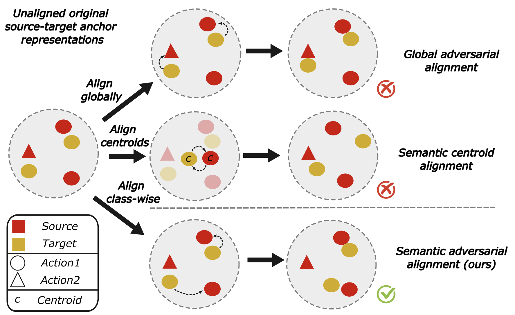
Recent advances in the field of video understanding have played a critical role in the surge of novel video-based applications – e.g., video indexing, summarization, recommendation, or surveillance. A critical task of this field is Temporal Action Localization (TAL), which involves identifying actions in a video consisting of both their time intervals and action categories. This is particularly difficult given the inherent variabilities of videos. These can be presented, among others, in the form of appearance variability – e.g. induced by differences in the kitchen – or as acquisition variability – e.g. different acquisition devices, lighting conditions, or acquisition viewpoints. All in all, these prompt a certain degree of confusion between similar actions to be discriminated.

Traditionally, fully supervised methods attempt to address this issue by leveraging enough training data to cover all the possible sources of variability. Unfortunately, this becomes virtually impossible when dealing with realistic scenarios. This compels these methods to operate under the influence of unseen data variations – i.e., domain gaps –, which exposes them to a considerable decline in performance. Overcoming this typically involves relabeling data from the new domain, so as to retrain and adapt the model. Unfortunately, this approach is impractical due to the considerable time and resource consumption involved, a challenge exacerbated when dealing with high-dimensional inputs like videos.

Unsupervised Domain Adaptation (UDA) has recently become a hot topic given its potential to leverage unlabelled data to mitigate this domain-induced degradation [17, 41, 21]. Unfortunately, despite its considerable success in image-based tasks [11], the application of UDA to video understanding remains underexplored. In fact, to the best of our knowledge, no prior work addresses UDA for TAL setups. The closest proposal is SSTDA [8], which approaches the problem of action segmentation. This focuses on making per-frame (namely dense) action predictions, tackling datasets where no concurrent actions take place [15, 29]. Hence, not being able to deal with sparse detections nor simultaneous intersection of labels.

Consequently, in this paper, we propose the first Unsupervised Domain Adaptation method for sparse detection on TAL, which we name Semantic Adversarial unsupervised Domain Adaptation or SADA for short. Our goal is to minimize the discrepancy between feature representations of a labeled source domain and an unlabelled target domain. These features are extracted with a multi-resolution architecture [49] that we couple with a novel adversarial loss that improves the limitations of existing UDA works. Concretely, existing works normally align domain distributions globally [17]. We propose instead to use pseudo-labeling [30] to assign an action or background (no action) class to each feature representation. With this, our loss factorizes the global adaptation strategy into independent per-class and background alignments – i.e., aligning each action’s distribution across both domains. This results in a more sensitive alignment strategy compared to a global distribution approach, less prone to feature misalignment and, as we will show, better performing.

Assessing the effectiveness of unsupervised domain adaptation methods for video understanding is a challenging, still unresolved task. Existing proposals on action segmentation [8] follow a subject-based strategy where they aim to adapt a model to new unseen subjects. Here we refer to subject as a person appearing in a video. Nevertheless, little data is normally available from a single subject, which inevitably requires grouping several of them for training. This allows the model to generalize over the subject variability under study, making it unsuitable to test for domain adaptation. We overcome these limitations by proposing a novel comprehensive suite of 6 new benchmarks for sparse TAL based on EpicKitchens100 [14] dataset. These study appearance and acquisition domain shifts, yielding a fine-grained and reliable evaluation of the model’s ability to operate on new unseen domains. This comprehensive benchmark allows us to demonstrate that our approach mitigates the performance degradation, improving by a large margin the existing fully supervised (namely source-only) and unsupervised domain adaptation-based proposals.

In short, our main contributions are three-fold:

1. We propose for the first time an unsupervised domain adaptation method suitable for sparse detection scenarios on TAL.

2. We introduce a novel adversarial loss that factorizes standard global alignment into independent class- and background-wise alignments (see Fig. 1).

3. We present a new set of benchmarks to test sparse detection scenarios when facing 6 different domain shifts, achieving state-of-the-art results in all of them.

2 Related work

Temporal Action Localization. At the time of this writing, most of the literature on the task of Temporal Action Localization follows a traditional source-only approach. In other words, they restrict the models’ visibility solely to a training domain, while other domains seen during testing are not available. These works can be categorized as follows: (1) Anchor-based methods [6, 31, 32, 46, 51, 3, 62, 49] propose a two-stage pipeline, consisting of a proposal generation and classification. The first applies heuristic methods – e.g., uniform sampling [3, 6, 62, 49] or action boundaries’ grouping [66, 65] – to generate a dense set of proposals – i.e., temporal segments. In the second stage, they leverage a learnable classifier to predict the corresponding action class and localization offsets of every anchor. Our work falls into this category motivated by the recent success of these methods achieving state-of-the-art results in many TAL benchmarks [24, 64, 14] (2) Anchor-free methods [50, 33, 32, 61] avoid this two-stage approach making per-frame predictions of their corresponding action labels. These methods, however, often suffer from a tendency towards over-segmentation given the potential discrepancy between neighboring frames. Consequently, they require often complex smoothing techniques to improve the boundary predictions [8] (3) Query-based methods [52, 35, 36] recently emerged as an alternative paradigm that follows the principles presented by [4]. This approach exploits the use of a Transformer encoder-decoder architecture [55] to learn a fixed small set of queries given refined video features, each identifying one potential action segment. Intuitively, this results in a non-heuristic-based proposal generation. This comes with the limitation of an increased rigidity, as the number of proposals needs to be fixed beforehand.

Unsupervised Domain Adaptation. Domain Adaptation techniques emerge as an effective solution to bridge the gap between data collected from a source and a target distribution, respectively. A large suite of approaches has been proposed to perform this alignment between the labeled and the unlabeled domains – e.g., discrepancy minimization [28, 60], entropy minimization [19, 59], contrastive learning  [26] or domain normalization [56]. The most popular approach is arguably the use of adversarial training methods [17, 41, 22, 54, 38, 21], which incorporate a domain classifier trained to discern if the samples come from the source or the target domain, in a min-max fashion. This results in the computation of domain-invariant embeddings [12]. Despite convenient, the simplicity of these methods might degrade the quality of the alignment [30], as they potentially align embeddings of source and target domain that represent different semantic information – e.g., different class labels. Few works have been proposed to do this alignment in a more sensitive way [30]. We highlight the importance of [58], proposing to minimize instead the distance of per-class centroids, computed as the mean of the set of predicted feature embeddings of a given class. Its effectiveness, however, relies on the assumption that the data is distributed somewhat homogeneously around the center, as otherwise, the centroids are not necessarily meaningful. In our work, we couple the advantages of both adversarial domain adaptation and semantic alignment and propose for the first time a pure adversarial semantic loss that yields domain invariant representations in a semantically meaningful way, without making explicit assumptions of the distributions (see Fig. 1).

Unsupervised Domain Adaptation for TAL: Despite the considerable success of UDA methods, their applicability has been mostly restricted to image-based scenarios [11] such as image classification [20, 17, 37, 41, 48], object detection [9, 42] or semantic segmentation [47, 23]. Much less attention has been dedicated to video-based applications such as action recognition [7, 25, 43] or spatio-temporal action segmentation [1, 40]. To the best of our knowledge, at the time of this writing, there is no direct comparison with our work focusing on sparse Temporal Action Localization. The closest work is SSTDA [8] that applies unsupervised domain adaptation for Action Segmentation. SSTDA proposes the use of two global-distribution-based auxiliary tasks to jointly align cross-domain feature spaces. Unlike our proposal, their work falls into the category of anchor-free, making per-frame action predictions. This restricts its applicability to action segmentation scenarios, where current datasets [15, 29] are designed to deal with frame-based single-action classification. In our work, we overcome this limitation by leveraging an anchor-based architecture that enables a natural adaptation to more realistic multi-label scenarios.

3 Method

Figure 2: Overview of the main model architecture of SADA. This takes as input videos from a Source and a Target domain, which are both fed to a shared multi-resolution feature extractor pyramid. The output embeddings of both of these domains are then aligned using the semantic alignment loss, SADA. This is done with a level and class-wise domain discriminator of the filtered embeddings, based on GT information and pseudo labels, for the source and target domains, respectively. Finally, the resulting domain invariant representations of the source domain are used to train a classification and localization head to learn the underlying task.

3.1 Problem definition and notation

In this paper, we address the problem of unsupervised domain adaptation for TAL. For this, we define a source domain $\mathcal{S}$ and a target domain $\mathcal{T}$. Domain $\mathcal{S}$ consists of $N_{\mathcal{S}}$ labeled input videos $\{(V_{k}^{\mathcal{S}},y_{k}^{\mathcal{S}})\}_{k=1}^{N_{\mathcal{S}}}$, where each video $V_{k}^{\mathcal{S}}$ is a sequence of $T$ frames $(X_{k,1},\dots,X_{k,T})$ with $X_{k,t}\in\mathbb{R}^{H\times W\times C}$. Here $y_{k}=(b_{k},e_{k},c_{k})$ contains the begin, end, and class actions of the ground-truth (GT) segments of the video, respectively. The target domain $\mathcal{T}$ is similar to $\mathcal{S}$ but lacks the GT information. Concretely, it consists of $N_{\mathcal{T}}$ unlabeled input videos $\{V_{k}\}_{k=1}^{N_{\mathcal{T}}}$. Our goal is to train a model that can identify the action segments, including both segment coordinates and action labels, in videos from domain $\mathcal{S}$, while minimizing the performance degradation on the unlabeled domain $\mathcal{T}$.

3.2 Framework overview

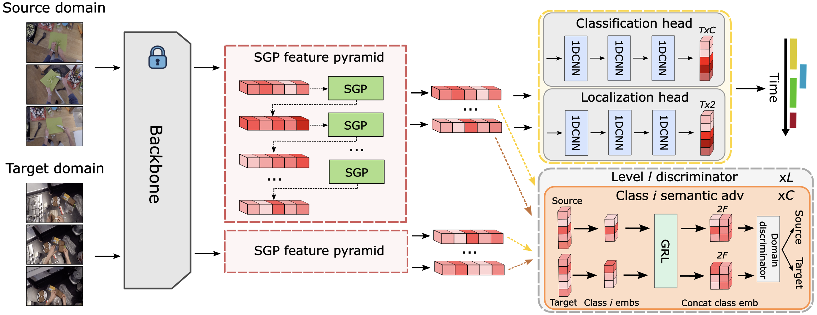
In this work, we propose a model based on a feature pyramid and a classification and localization head (see Fig. 2). This architecture is coupled with a novel semantic adversarial loss that aligns the embeddings of the source and target domain in a semantically meaningful way. More in detail, the model takes as input two videos from domain $\mathcal{S}$ and $\mathcal{T}$, respectively. The model first processes the raw input videos using a frozen pre-trained video backbone. The resulting embeddings of both domains are then passed through a shared SGP pyramid [49] that outputs a set of multi-resolution anchor embeddings for each of the predefined resolution levels. The main goal of our model is to make these anchor embeddings domain invariant. For this, we introduce a level-wise semantic adversarial loss that learns in an adversarial manner to align the embeddings of both domains belonging to a given action class $i$ at a given resolution level $l$. Recall that GT information is only available for domain $\mathcal{S}$, therefore we rely on the use of pseudo labeling techniques [30] to infer the probable class labels of the data from domain $\mathcal{T}$. Finally, we use the domain invariant anchors of domain $\mathcal{S}$ to train a classification and localization head that learns the underlying tasks in a standard supervised fashion. In short, this permits to learn a classification and localization head that minimizes the decline of performance when applied to the unseen domain $\mathcal{T}$.

3.3 Backbone and SGP pyramid

Our model first takes two input videos $V^{\mathcal{S}}$ and $V^{\mathcal{T}}$ of both domains $\mathcal{S}$ and $\mathcal{T}$. For simplicity, both videos $V^{\mathcal{S}}$ and $V^{\mathcal{T}}$ have length $T$, which we enforce using padding. The method then processes the two raw videos applying a frozen pre-trained backbone – e.g., I3D [5], Slowfast [16]. This permits to extract, in an effective way, temporal cues of the video into a set of refined video features. These embeddings are then fed to an SGP feature pyramid [49] which combines the use of SGP blocks and the progressive downsampling of the temporal length by a ratio of $2$. This outputs a set of multi-resolution anchor embeddings $Z^{\mathcal{S}}=\{Z_{l}^{\mathcal{S}}\}_{l\in L}$ and $Z^{\mathcal{T}}=\{Z_{l}^{\mathcal{T}}\}_{l\in L}$, for the two domains, respectively. Here $L$ denotes the set of predefined resolution levels and $Z_{l}\in\mathbb{R}^{T_{l}\times F}$ the anchor embeddings of level $l$ of a given domain. Concretely, this permits to obtain embeddings for a set of uniformly sampled anchors at each of the $l\in L$ resolution levels. The use of a multi-resolution model is favorable to naturally adapt to different action lengths.

3.4 Classification and localization head

To learn the underlying TAL task, we train in a fully supervised manner a classification and localization module with the labeled source domain $\mathcal{S}$. Due to the anchor-based nature of our model, we first require a matching strategy between the set of candidate anchors to the actual GT segments. For this, we follow a center sampling strategy [53, 63, 62, 49]. In other words, for a given level $l$, we define an anchor as positive if the time instant $t$ that it represents is near the center of an action. All the rest are marked as negative. We define $\mathcal{B}_{l},\mathcal{E}_{l}$ and $\mathcal{C}_{l}$ as the begins, ends and action classes of their matching GT segments. We identify negative anchors by assigning them to action class 0.

With this, we design a classification head $H_{cls}:\mathbb{R}^{T_{l}\times F}\rightarrow\mathbb{R}^{T_{l}\times C}$ that maps each of the anchor embeddings to their class distribution. More specifically, we model this as a sequence of 1D convolutions, and train it using a sigmoid focal loss (SFL) [34] as follows:

$$\small\mathcal{L}_{SFL}^{l}=SFL(H_{cls}(Z^{\mathcal{S}}_{l}),\;\mathcal{C}_{l}).$$ (1)

Similarly, we model a localization head $H_{loc}:\mathbb{R}^{T_{l}\times F}\rightarrow\mathbb{R}^{T_{l}\times 2}$ identically as $H_{cls}$, which predicts the begin-end offsets. We thus define the localization loss as a standard mean squared error (MSE) loss over the positive samples only:

$$\small\mathcal{L}_{loc}^{l}=MSE(H_{loc}(Z_{l{{}_{+}}}^{\mathcal{S}}),\;(\mathcal{B}_{l_{+}}\,||\,\mathcal{E}_{l_{+}})),$$ (2)

where $l_{+}$ refers to the positive samples from the $l$-th level only and $||$ to the concatenation operation. This yields the final task loss defined as:

$$\small\mathcal{L}_{task}=\lambda_{cls}\;\sum_{l\in L}\mathcal{L}_{SFL}^{l}+\lambda_{loc}\;\sum_{l\in L}\mathcal{L}_{loc}^{l}.$$ (3)

Here $\lambda_{cls}$ and $\lambda_{loc}$ are tunable parameters that control the importance of each of the two losses, respectively.

3.5 Our proposal: Semantic adversarial multi-resolution alignment

One of the main contributions of this paper is the design of a novel adversarial-based loss that we name SADA loss, which attempts to overcome the limitations of the extensively used global adversarial loss [17]. Traditional adversarial domain adaptation relies on the idea of designing a domain classifier that learns to identify the domain that each of the embeddings belongs to. The rest of the model learns concurrently the opposite objective, which, as shown by [17], results in the learning of the domain invariant representations. While this approach has been shown to be effective in other fields – e.g., image classification, object detection – we find that its performance in a more challenging setup like TAL still presents important challenges. One of the main issues, as argued by [30] is that this loss often suffers from feature misalignment which greatly declines the model’s performance. This refers to the cases where these methods align embeddings of non-matching class labels – e.g., aligning embeddings of domain $\mathcal{S}$ of an action $i$ with embeddings of domain $\mathcal{T}$ of a class $j$.

3.5.1 Local adversarial alignment

To fix this feature misalignment in realistic scenarios like TAL, we propose an alternative adversarial loss formulation that provides a finer-grained alignment. This loss first attempts to perform a local class-aware alignment. This is, for every given resolution level $l$, we group the anchor embeddings of $\mathcal{S}$ and $\mathcal{T}$ corresponding to an action label $i$. This is straightforward for the source domain as we have the GT information. For the target domain, we use a hard-pseudo labeling strategy [30] that classifies a given embedding as class $i$ if this is the highest-confidence score of the predicted class distribution, and this is above a threshold $\alpha$. Formally we define the hard pseudo-label of a given anchor $z$ as:

$$\small\hat{c}_{z}={\begin{cases}\underset{i}{\mathrm{argmax}}\;P_{l}[z,i]&\text{if }P_{l}[z,i]>\alpha\\ 0&\text{otherwise},\end{cases}}$$ (4)

where $P_{l}=H_{cls}(Z^{\mathcal{T}}_{l})\in\mathbb{R}^{T_{l}\times C}$ are the predicted class probabilities of the anchors. We assign a class $0$ to the background anchors – those not assigned to any class. From this, we obtain the new grouped embeddings of source and target domain of class $i$ on level $l$ as:

$$\small A_{i}^{l}=\{Z_{l}^{\mathcal{S}}[z]\;:\;c_{z}=i\}_{z\in T_{l}},$$ (5)

$$\small B_{i}^{l}=\{Z_{l}^{\mathcal{T}}[z]\;:\;\hat{c}_{z}=i\}_{z\in T_{l}},$$ (6)

for $A_{i}^{l}\in\mathbb{R}^{T_{l,i}\times F}$, $B_{i}^{l}\in\mathbb{R}^{T_{l,i}\times F}$. Also, $c_{z}$ is the GT action label of anchor $z$ and $\hat{c}_{z}$ is its computed pseudo-label from Eq. 4. We then adversarially train a domain classifier $D:\mathbb{R}^{2F}\rightarrow\{0,1\}$ to identify the domain of each of these embeddings using a binary cross entropy (BCE) loss:

$$\small\mathcal{L}_{local}^{l}=\sum_{i=1}^{C}(\mathcal{L}_{\text{\tiny{BCE}}}(D(A_{i}^{l}\,||\,E_{i}),d_{\mathcal{S}}))+(\mathcal{L}_{\text{\tiny{BCE}}}(D(B_{i}^{l}\,||\,E_{i}),d_{\mathcal{T}})),$$ (7)

where $d_{\mathcal{S}}$ and $d_{\mathcal{T}}$ are the labels of each of the domains. Following [17], we introduce a Reverse Gradient Layer (GRL) before the discriminator $D$ to invert the gradients sign which creates the min-max game where the feature extractor learns to confuse the discriminator. We condition the discriminator to class $i$ using a learnable class embedding $e_{i}\in\mathbb{R}^{F}$ that we replicate for every selected anchor into an embedding $E_{i}$. See the Supp. for an ablation that justifies this design decision.

3.5.2 Local and global alignment: SADA

Eq. 7 aligns solely the anchor embeddings that are classified as one of the $C$ classes, but what happens with the background embeddings that fall below the threshold $\alpha$? In this case, the loss completely ignores their influence, yielding a suboptimal partial alignment – as shown in Sec. 4.

To overcome this issue, we propose our final SADA loss which attempts to combine the best of both global alignment loss [17] and Eq. 7. For this, we introduce a new loss term for the background embeddings as follows:

$$\small\begin{aligned} \mathcal{L}_{bkg}^{l}=&\mathcal{L}_{\text{BCE}}(D(A_{0}^{l}\;||\;E_{0}),d_{\mathcal{S}})+\mathcal{L}_{\text{BCE}}(D(B_{0}^{l}\;||\;E_{0}),d_{\mathcal{T}})\\ \end{aligned},$$ (8)

where again $A_{0}^{l}$ and $B_{0}^{l}$ are the selected background anchors, and $E_{0}\in\mathbb{R}^{F}$ is the learnable background embedding. Coupling Eq. 7 and Eq. 8 yields the final formulation of our proposed loss, combining class-wise alignment with the background anchors alignment. Formally:

$$\small\mathcal{L}_{sada}=\sum_{l\in L}\lambda_{l}\;(\mathcal{L}_{local}^{l}+\mathcal{L}_{bkg}^{l}),$$ (9)

where $\lambda_{l}$ is a hyper-parameter that regulates the importance of level $l$ on the final alignment loss.

3.6 Training

During training, we formulate the final loss as a min-max game where the main model architecture is optimized over the classification and localization loss while maximizing the adversarial loss. In parallel, the discriminator model $D$ attempts to minimize the discriminator loss only. Formally,

$$\small\mathcal{L}=\lambda_{task}\mathcal{L}_{task}+\lambda_{sada}\mathcal{L}_{sada}.$$ (10)

Note again $\mathcal{L}_{task}$ is optimized with domain $\mathcal{S}$ while $\mathcal{L}_{sada}$ promotes the alignment between both domains $\mathcal{S}$ and $\mathcal{T}$. Moreover, $\lambda_{task}$ and $\lambda_{sada}$ are tunable parameters that control their influence on the loss.

4 Datasets and experiments

In this section, we present a novel comprehensive benchmark to evaluate the task of UDA for TAL. Our setup, for the first time, goes beyond action segmentation and evaluates the adaptation to different domain shifts in more realistic scenarios with sparse multi-label annotations. We then showcase the effectiveness and competitiveness of our model over the state-of-the-art methods together with several relevant ablations.

4.1 Experimental setup

Evaluating domain adaptation-based methods in the context of video understanding is a challenging issue that requires the definition of a reasonable domain gap and identifying a sufficiently large set of intersecting action classes. Dividing existing datasets into different domains that comply with these conditions often restricts the amount of data to learn and adapt. SSTDA [8] approaches this problem on GTEA [15] and Breakfast [29] by defining a subject-based partitioning where they aim to adapt the model to new unseen subjects. However, as little data is available from a single subject in those datasets, they group several users for training. This allows the model to generalize over the subject variability under study, making it unsuitable to test for domain adaptation. Closely related to our work, TranSVAE [57] defines a source-target for video classification based on EpicKitchens100 [14]. They split the data into three different kitchens as different domains and perform cross-kitchen evaluation, limiting even further the amount of data in each domain.

Figure 3: Overview of the 6 proposed experimental setups. Scenarios 1 and 2 evaluate the videos from the original EK55. They define the dark-counter and white-counter kitchens as Source, respectively, and the rest as Target. Scenarios 3 and 4 are similar except that they consider only the newest videos from EK100. Finally, Scenarios 5 and 6 use the old videos as Source and the new videos as Target, and vice versa.

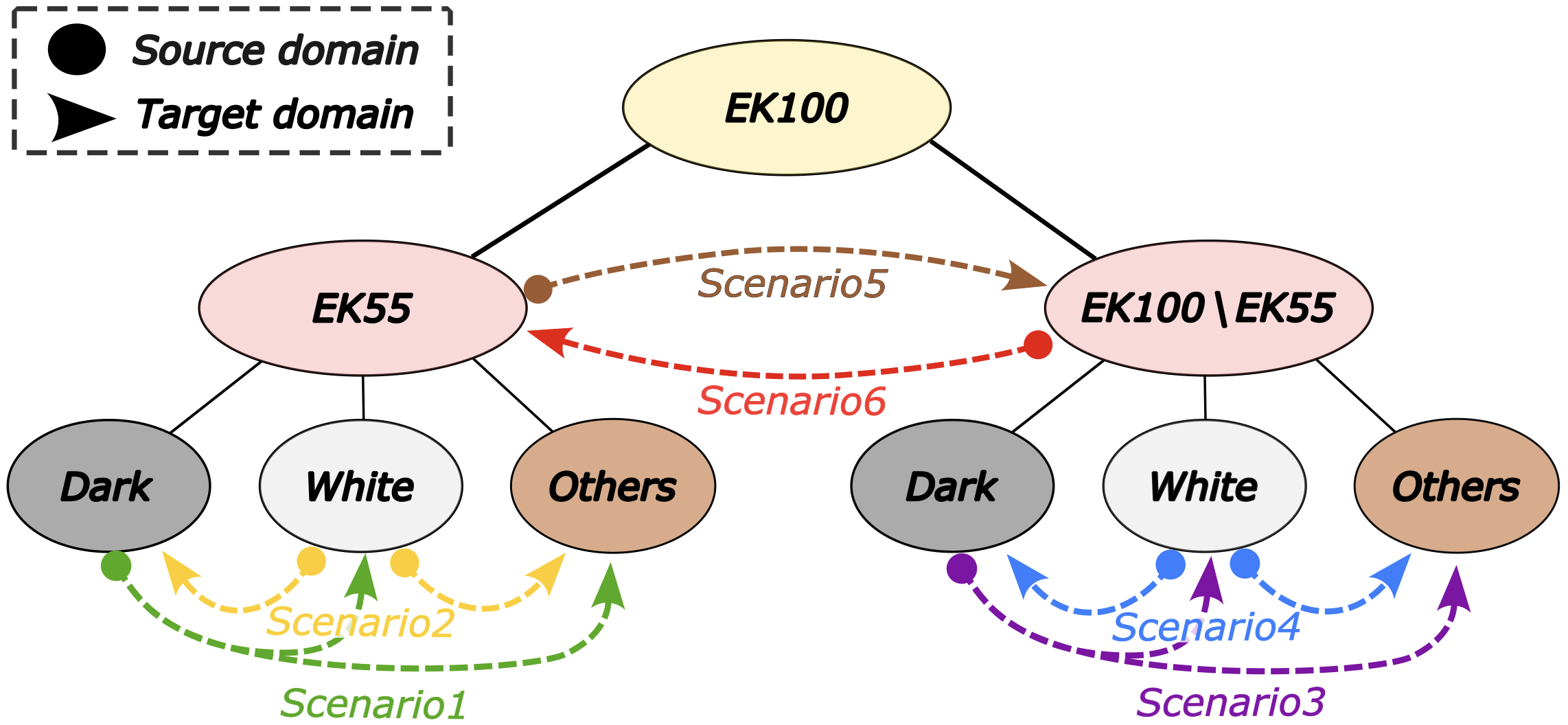
A new benchmark for UDA on sparse TAL. To overcome these limitations, we propose a set of 6 different benchmarks for sparse TAL based on the EpicKitchen100 [14]. EpicKitchen100 presents an ideal base for our tasks as it has become a gold standard to evaluate complex sparse detection scenarios on long egocentric videos (up to 45 minutes). We identify two domain gaps in this dataset: an appearance domain shift based on the different colors of the kitchen counters; and an acquisition domain shift that results in the differences of lighting and camera conditions when extending EpicKitchens55 [14] into its new version EpicKitchens100 [14]. This permits to define a rich set of benchmarks that provide a more fine-grained and comprehensive evaluation. Importantly, this strategy is also suitable for single-source settings which do not allow an easy generalization over the shift under study. For example, if a model is trained with dark-counter kitchens only, it cannot easily generalize to white-counter kitchens.

More in detail, we introduce 4 different benchmarks that derive from the aforementioned appearance shift. For this, we first define two different splits of EK55 and {EK100 \EK55} videos according to [14], put more plainly old versus new videos. We then further split each of them according to the color of the kitchen counter and define 4 different setups of single-source domain and multi-target domain – i.e., dark $\rightarrow$ white and other kitchens; and white $\rightarrow$ dark and other kitchens, for old and new videos, respectively. Similarly, given the two splits between EK55 and {EK100 \EK55} videos, we propose 2 additional setups of EK55 $\rightarrow$ {EK100 \EK55} and {EK100 \EK55} $\rightarrow$ EK55. These measure the adaptability to different acquisition conditions – i.e., lighting and camera conditions. We refer to the Supp. for more details on these setups.

One final important consideration is that EpicKitchens100 [14] exhibits a very strong long-tail label distribution, where the vast majority of its 97 actions represent only a marginal percentage of the overall data. Adapting domain adaptation methods to these long tail distributions falls beyond the scope of this paper and most of the existing literature. For this reason, we limit our evaluation to the 10 majority classes representing $80\%$ of the original dataset. This still results in a very complex task proof of which is that the best-performing models to date attain less than a 30% mAP [62, 49].

4.2 Experimental results

Scenario	Model	mAP10%	mAP20%	mAP30%	mAP40%	mAP50%	Avg
B $\rightarrow$ {all \B} (EK100 \EK55)	Actionformer [62]	28.11	26.94	24.89	21.43	16.51	23.57
	Tridet [49]	29.47	28.32	25.50	21.99	16.34	24.32
	Ours (SADA)	32.69	31.49	29.17	25.51	19.72	27.72
B $\rightarrow$ {all \B} (EK55)	Actionformer [62]	30.21	28.73	26.39	22.60	17.09	25.00
	Tridet [49]	29.87	28.39	25.97	22.06	16.94	24.65
	Ours (SADA)	31.60	30.29	28.22	24.47	18.98	26.72
W $\rightarrow$ {all \W} (EK100 \EK55)	Actionformer [62]	33.52	32.31	29.84	26.48	20.11	28.45
	Tridet [49]	34.01	32.52	30.07	26.40	19.78	28.55
	Ours (SADA)	34.86	33.73	31.16	27.45	21.46	29.73
W $\rightarrow$ {all \W} (EK55)	Actionformer [62]	27.46	26.54	24.61	21.85	17.19	23.53
	Tridet [49]	30.03	28.97	26.96	23.48	18.18	25.52
	Ours (SADA)	31.54	30.68	28.77	25.52	20.22	27.34

Table 1: Comparison of our proposal SADA with the state-of-the-art for the 4 different appearance-shift scenarios (1-4).

Scenario	Model	mAP10%	mAP20%	mAP30%	mAP40%	mAP50%	Avg
EK55 $\rightarrow$ (EK100 \EK55)	Actionformer [62]	22.87	21.87	20.10	17.23	13.33	19.08
	Tridet [49]	24.77	22.93	21.49	19.09	15.15	20.48
	Ours (SADA)	25.93	25.06	23.47	20.45	16.12	22.21
(EK100 \EK55) $\rightarrow$ EK55	Actionformer [62]	22.16	21.22	19.71	17.44	14.08	18.92
	Tridet [49]	22.47	21.57	20.19	17.87	14.41	19.30
	Ours (SADA)	23.94	22.95	21.47	19.16	15.24	20.55

Table 2: Comparison of our proposal SADA with the state-of-the-art for the 2 different acquisition-shift scenarios (5-6).

In this section, we present the main experimental results evaluating appearance and acquisition shifts. All these experiments follow the standard transductive unsupervised DA protocol [44, 10], and report the mean average precision (mAP) at different intersection over union (IOU) thresholds ($10\%-50\%$).

Appearance shift scenarios. In Tab 1 we present the results obtained in the 4 different scenarios that we designed to evaluate the performance of our method when facing different domain shifts induced by changes in the background information. In this table, we compare our method to Actionformer [62] and TriDet [49], the two best-performing methods on EpicKitchens100 dataset [14] for TAL at the time of this writing.

In the first two experiments where we use dark-counter kitchens to define the source domains, we observe a consistent relative improvement of SADA over the chosen baseline methods of up to $13.98\%$. We observe a similar behavior for the 2 scenarios with white-counter kitchens acting as source, where our model improves the baselines with up to $7.12\%$.

Acquisition shifts. Similarly, Tab. 2 shows the results for the two proposed scenarios evaluating acquisition domain shifts – e.g., camera and lighting conditions. In the first scenario where we define old videos as the source domain, we observe a considerable relative improvement of $8.45\%$ over TriDet [49]. This improvement becomes more prominent comparing it to ActionFormer which we improve by $16.4\%$. The results indicate that the opposite setup presents a much more challenging scenario. In this case, our method attains a slightly more moderate yet consistent improvement of up to $6.48\%$.

4.3 Ablation studies

Comparing to other domain adaptation methods. In Sec. 4.2 we showed the performance increase that SADA yields with respect to SOTA source-only methods on our 6 setups. This comparison does not include any domain-adaptation-based method as our proposal is the first one suitable for sparse temporal detection setups. Nevertheless, this raises the question of how other domain adaptation methods would perform if coupled with our chosen multi-resolution architecture? In Tab. 3 we conduct several relevant experiments on Scenarios 1 and 3, defining the source domain as new and old black-counter kitchens, respectively. We refer to the Supp. for the ablations on other benchmarking scenarios.

B $\rightarrow$ {all \B} (EK100-EK55)
Model	mAP {10,30,50}%			Avg
Source-only	30.03	26.62	17.79	24.81
DANN [18]	30.48	27.07	18.12	25.22
Semantic centroids [58]	31.07	27.16	17.21	25.14
SSTDA [8]	27.16	24.32	16.30	22.59
Ours (SADA)	32.69	29.17	19.72	27.19
B $\rightarrow$ {all\B} (EK55)
Model	mAP {10,30,50}%			Avg
Source-only	30.74	27.23	18.07	25.34
DANN [18]	30.87	27.45	18.29	25.97
Semantic centroids [58]	30.88	27.44	18.25	25.52
SSTDA [8]	29.50	26.87	17.13	24.50
Ours (SADA)	31.60	28.22	18.98	26.27

Table 3: Ablation study on Scenarios 1 and 2, comparing the performance of SADA with relevant domain adaptation methods coupled in our proposed architecture to ensure a fair comparison.

For this, we benchmark the performance of our method with its source-only variant. We also include a direct comparison with adaptations of several domain-adaptation methods like DANN [18], semantic centroid alignment [58], and SSTDA [8], the closest work to our proposal.

As observed in Tab. 3, in the first considered scenario our method consistently yields a better performance than any of the evaluated domain adaptation methods. More specifically, we find that the first two alternatives yield only a marginal relative improvement over the source-only variant of up $1.65\%$, whereas SSTDA [9] obtains a considerable decay of performance. For the latter, we hypothesize that this is due to the change of paradigm. Despite its original success, SSTDA was designed for frame-level prediction setups, inherently different from the task at hand. We observe a similar behavior in the second scenario, where DANN seems to work considerably better than the other baselines, but still well below our proposal, SADA.

Analysis of our loss. In this section we ablate over different variants of our proposed SADA loss (see Eq. 9). Concretely, in Tab. 4 we study the effect of class-wise distribution alignment (Eq. 7), global distribution alignment (DANN [18]) and semantic background alignment (Eq. 8).

In this regard, we highlight that the global adaptation seems to consistently improve upon aligning only background embeddings. This is because the latter yields only a partial alignment of the embeddings, not considering class anchors. Therefore, a rougher yet complete adaptation might seem beneficial.

We also observe that aligning local class-wise distributions has a considerable positive effect, especially in the first scenario. Its effect, however, considerably decreases when combined with a global alignment [18], as all the class anchors are then subject to the concurrent alignments of domain-level and class-wise distributions. This observation is also consistent with the performance decrease that we observe when combining global and background alignment, which again suggests that the concurrent alignment of background embeddings with two adaptation losses is harmful to performance.

Finally, we observe that we consistently obtain the best results when the local alignment loss is coupled with the complementary (non-overlapping) background loss – i.e., SADA loss – indicating that this semantic fine-grained, yet complete, alignment is the most desirable approach. We refer to the Supp. for a more complete class-wise analysis.

B $\rightarrow$ {all \B} (EK100-EK55)
Local	Global	Bkg	mAP {10,30,50}%			Avg
			30.03	26.62	17.79	24.81
	$\textpdfrender{TextRenderingMode=FillStroke,LineWidth=1.0pt,}{\checkmark}$		30.48	27.07	18.12	25.22
		$\textpdfrender{TextRenderingMode=FillStroke,LineWidth=1.0pt,}{\checkmark}$	30.34	26.66	17.04	24.68
	$\textpdfrender{TextRenderingMode=FillStroke,LineWidth=1.0pt,}{\checkmark}$	$\textpdfrender{TextRenderingMode=FillStroke,LineWidth=1.0pt,}{\checkmark}$	29.76	26.63	17.52	24.64
$\textpdfrender{TextRenderingMode=FillStroke,LineWidth=1.0pt,}{\checkmark}$			31.36	28.01	18.67	26.01
$\textpdfrender{TextRenderingMode=FillStroke,LineWidth=1.0pt,}{\checkmark}$	$\textpdfrender{TextRenderingMode=FillStroke,LineWidth=1.0pt,}{\checkmark}$		30.09	26.88	17.43	24.80
$\textpdfrender{TextRenderingMode=FillStroke,LineWidth=1.0pt,}{\checkmark}$		$\textpdfrender{TextRenderingMode=FillStroke,LineWidth=1.0pt,}{\checkmark}$	32.69	29.17	19.72	27.19
B $\rightarrow$ {all \B} (EK55)
Local	Global	Bkg	mAP {10,30,50}%			Avg
			30.74	27.23	18.07	25.34
	$\textpdfrender{TextRenderingMode=FillStroke,LineWidth=1.0pt,}{\checkmark}$		30.87	27.45	18.29	25.97
		$\textpdfrender{TextRenderingMode=FillStroke,LineWidth=1.0pt,}{\checkmark}$	30.97	27.64	18.39	25.67
	$\textpdfrender{TextRenderingMode=FillStroke,LineWidth=1.0pt,}{\checkmark}$	$\textpdfrender{TextRenderingMode=FillStroke,LineWidth=1.0pt,}{\checkmark}$	30.36	26.82	18.01	25.06
$\textpdfrender{TextRenderingMode=FillStroke,LineWidth=1.0pt,}{\checkmark}$			30.82	27.57	18.30	25.56
$\textpdfrender{TextRenderingMode=FillStroke,LineWidth=1.0pt,}{\checkmark}$	$\textpdfrender{TextRenderingMode=FillStroke,LineWidth=1.0pt,}{\checkmark}$		30.30	26.98	17.85	25.04
$\textpdfrender{TextRenderingMode=FillStroke,LineWidth=1.0pt,}{\checkmark}$		$\textpdfrender{TextRenderingMode=FillStroke,LineWidth=1.0pt,}{\checkmark}$	31.60	28.22	18.98	26.27

Table 4: Ablation study of the effect of several modifications of our proposed SADA loss.

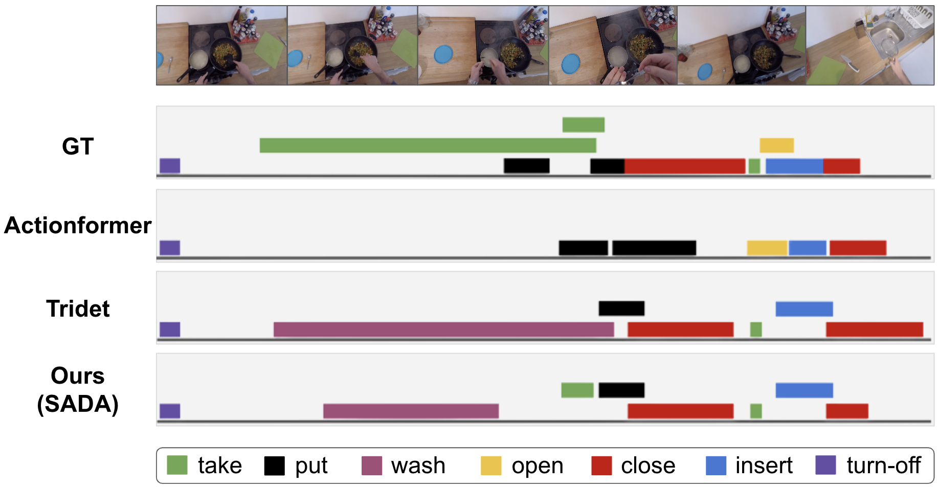
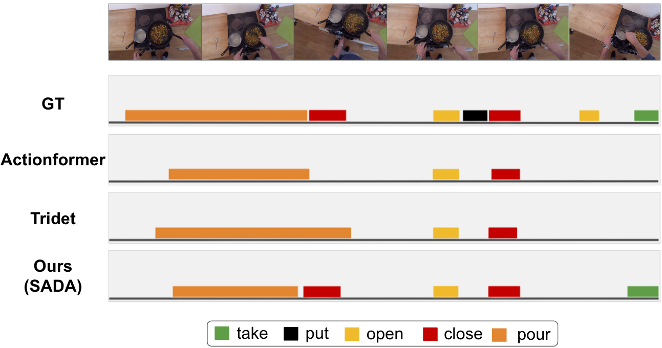
Qualitative analysis. We complement our quantitative results with a qualitative study. For this, we depict in Fig. 4 a segment visualization of our proposed method versus the chosen baseline models. In this visualization, we can observe that the Actionformer [62] misses many of the segments in the shown video clip ignoring all the take actions and mistaking a close action for a take. Tridet [49] performs better but misses all the take actions in the first half of the video while worsening the boundary prediction of the last close. SADA improves Tridet by predicting the second take action and considerably improving the boundary of the last close action.

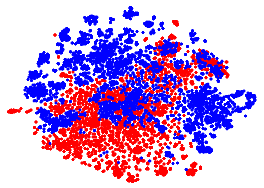
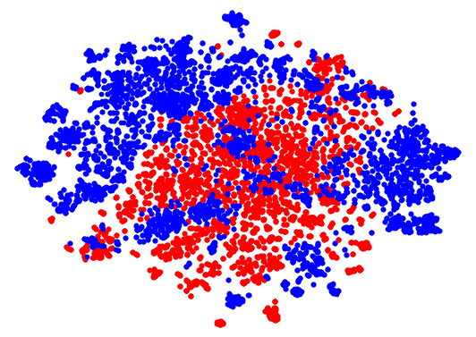
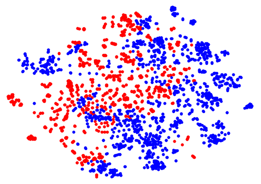
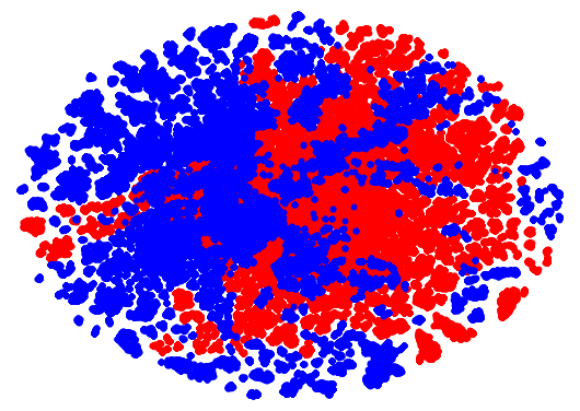
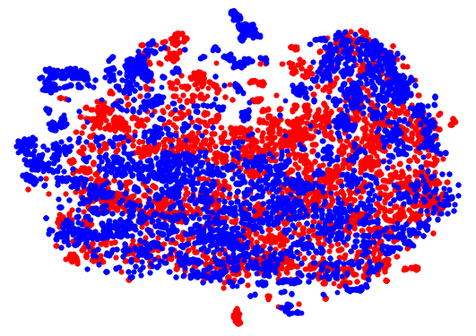
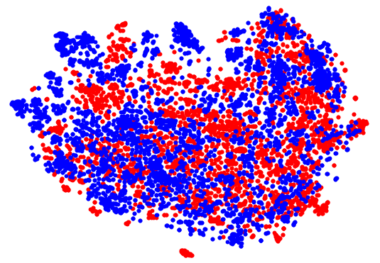
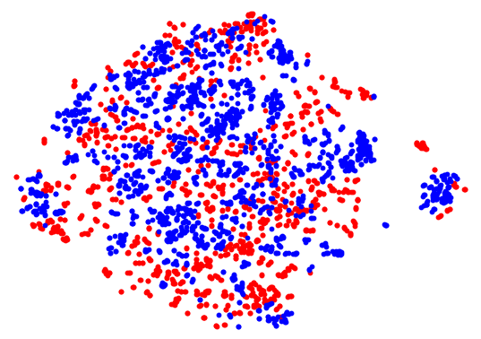
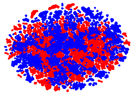
In Fig. 5 we also show the TSNE projections of the domain-invariant embeddings of SADA with respect to its source-only version. Given that our main contribution is an adversarial-based class-wise loss, we depict the TSNE plots of the 3 majority action classes (first 3 columns). Observe that the source only (top row) yields clearly unaligned distributions with scarce to no overlap in the projected space. Our method, in contrast, presents a considerable distribution mix improving the alignment of class-wise distributions across domains. Given the anchor-based nature of our method, we have numerous background anchors – i.e., not assigned to any true action label. As observed in the last column, these are also aligned by our method (resulting from Eq. 8) effectively aligning the entire data distributions but in a semantically sensitive way. We refer to the Supp. for the complete qualitative study.

Figure 4: Visualization of the predicted segments of our method and the chosen set of source-only baselines. We include on top the ground-truth (GT) segments as a reference.

(a) Class1(SO)

(b) Class2(SO)

(c) Class3(SO)

(d) Bkg(SO)

(e) Class1(DA)

(f) Class2(DA)

(g) Class3(DA)

(h) Bkg(DA)

Figure 5: TSNE plots of the source-only variation of our model (top row) and our proposed model (bottom row). Find in the first 3 columns the TSNE plots of action classes 1 to 3 of the source (red) and target (blue) domain anchors. The last column shows the plot of the background anchors, so those not assigned to any GT label.

5 Conclusions and limitations

In this work, we deal for the first time with Unsupervised Domain Adaptation on realistic Temporal Action Localization (TAL) scenarios. We propose a novel semantic adversarial loss that enables a more fine-grained distribution alignment compared to existing global-distribution-based approaches. Given the lack of suitable evaluation setups for this scenario, we propose a suite of 6 different benchmarks that provide a comprehensive assessment of the model performance across various domain shifts. These experiments indicate that our model yields a considerable improvement over state-of-the-art methods, which we support with extensive quantitative and qualitative results.
Limitations and future work. Despite the virtues of our proposed benchmarking scenarios, we leave as future work to study alternative cross-dataset setups including larger and different domain shifts, e.g. extreme viewpoint changes or motion. This would possibly require relabeling new datasets. We also plan on complementing these studies with long-tail scenarios, analyzing the effect of domain adaptation optimization in the presence of highly unbalanced data in terms of labels. We also leave as future work the analysis and possible benefits of the adaptation of our semantic adversarial loss to other domain adaptation problems, even to those not necessarily related to video tasks.

Supplementary Material

In this supplementary material, we first provide the implementation details needed to reproduce our work (see Sec. A). We then provide additional details of the description of Sec. 4.1 regarding our 6 proposed benchmarking scenarios (see Sec. B), which we complement with a visualization of the different scenarios (available in this link). In Sec. C we detail the necessary adaptations that we made on existing unsupervised domain adaptation (UDA) so that they could operate on our proposed setups. We then extend our qualitative analysis from Sec. 4.3, providing additional segment visualizations (see Sec. D.1 and this link) and an additional study of the effect of the alignment loss SADA on multiple resolution levels (see Sec. D.2). In Sec. E we provide empirical evidences that justify the choice of using learnable class embeddings. Find also in Sec. F an extension of the main-paper ablation from Sec. 4.2, where we present the experimental results for two additional scenarios. We complement these results with a more thorough study of the per-class performance of our model on multiple scenarios (see Sec. G). Finally, in Sec. H we ablate over the potential negative impact that the presence of negative anchors has on the performance of our model.

A Implementation details

Our implementation of SADA is based on the PyTorch [45] framework. SADA extracts video features using a frozen Slowfast [5] video backbone pre-trained on Kinetics [27]. This backbone is fed with raw videos from EpicKitchens100 [14] with a rate of $30$ FPS, a feature stride of $16$, and a maximum length of $2304$ ensured by either padding – for shorter videos – or random cropping. To ensure a fair comparison with [49], we also define the main feature extractor as a 6-level SGP feature pyramid [49] that follows a max pooling strategy and uses a downsampling rate of $2$ and an internal feature dimensionality of $1024$. We model the classification and localization heads as a sequence of three 1D-CNNs with a kernel size of $3$. These heads are shared across embeddings of different resolution levels. Finally, we introduce level-wise domain discriminators designed as a multi-layer perceptron (MLP) of depth $3$. The weights of the losses are tuned following a grid search strategy.

During training, the model first shuffles the videos of the source and target domain, respectively. It then feeds a batch of $2$ videos of each of the domains, resulting in a batch of $4$ videos per training iteration. Note that depending on the scenario under study, one of the domains may have more data than the other. For this reason, in each epoch we repeat the smaller domain until the other finishes, ensuring that all the data of each of the domains is leveraged at least once. Moreover, the model architecture is optimized for $50$ epochs using AdamW [39] with a learning rate of $1e-4$ with cosine decay and a warm-up phase of $5$ epochs.

During inference, we follow a similar approach to [62, 49] and define an exponential moving average of the trained model, which we update every iteration with an exponential decay of 0.999. Moreover, given the excess of final predictions, we use the standard SoftNMS [2] with an IOU threshold of 0.1, a minimum score threshold of 0.001, and a sigma value of 0.4.

B Extended benchmark description

In this section we describe in more depth the 6 different benchmarking scenarios that we propose in Sec. 4.1. For this, in Sec. B.1 we first briefly describe EpicKitchens100 [14], the base of all our benchmarks. We then illustrate in Sec. B.2 and Sec. B.3 the 2 different domain shifts that we identify, which we complement with a more detailed description of the specific scenarios derived from each of them.

B.1 Description EpicKitchens100

EpicKitchens100 [14] is a large-scale ego-centric dataset that has recently gained a lot of attraction in the Temporal Action Localization community to test for challenging detection scenarios. This dataset extends the previous version of the dataset, namely EpicKitchens55 [13]. This dataset contains videos of 32 subjects performing daily cooking activities – e.g., wash, put, open, close – in different kitchen environments. This results in 100 hours of non-scripted videos containing 20M frames annotated with 90K action segments.

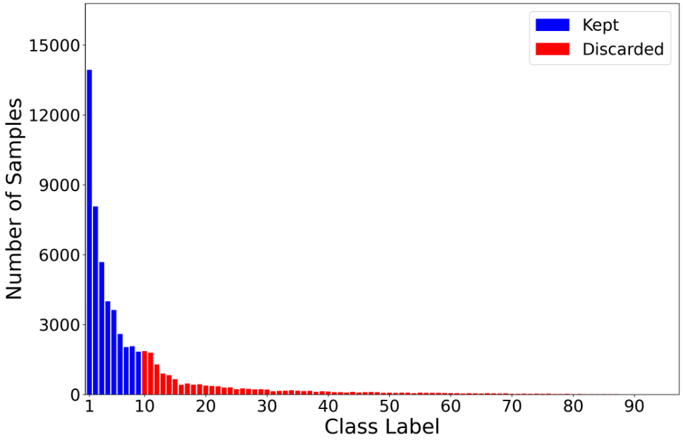
One of the key challenges of this dataset is the presence of 97 different actions, forming a very long tail action distribution. This inherent characteristic is however an issue that falls beyond the scope of this paper, given the important additional challenges that this poses in existing domain adaptation-based methods. For this reason, in all our experiments we consider only the 10 majority classes – i.e., take, put, wash, open, close, insert, turn-on, cut, turn-off and pour. As shown in Fig. A this pruning keeps most of the labeled action segments of the original dataset, concretely keeping up to $80\%$ of it (marked in blue in the histogram). Moreover, we find that this design decision does not diminish in a relevant way the challenging nature of this task. Proof of this is that the currently best-performing methods on this dataset – i.e., Actionformer [62] and Tridet [49]– still attained mAP metrics inferior to $30\%$ in all our proposed scenarios.

Figure A: Histogram of the number of GT action segments of every class. We also depict in blue the 10 majority classes –which we keep in our setups– while leaving as red the remaining class that we discard to avoid the long-tail action distribution problem.

B.2 Studying acquisition shifts

The first domain shift that we identify in the EpicKitchens100 [14] is what we call the acquisition shift. This shift refers to the changes induced by differences in the acquisition conditions of the videos. In the case of EpicKitchens100 [14] this results from the extension of the original dataset EpicKitchens55 [13]. The original dataset, concretely, was formed by 55 hours of non-scripted videos, and nearly 40K action segments. Hence, we find that this presents a suitable setup to define one domain as the old videos – recorded in the original EpicKitchens55 [13] – and the other formed by the new videos – recorded for the extended version. As argued by [14] this results in several important domain gaps that are captured by these data splits:

• Changes in the acquisition devices: The new videos that were recorded during the extension relied on a newer camera device. Importantly, this camera incorporates camera stabilization techniques. Fig. B visually depicts the improvement in the stability of new over old videos.

• Lighting conditions: Given the changes in the hour of the recording, these domains also present differences in the lighting conditions of the videos.

(a) Old videos

(b) New videos

Figure B: Visualization of the differences in camera stability between old and new videos. These images were obtained with differences of 3 frames, which correspond to a period of 0.1 seconds. We highlight with a red circle in 2(a) a reference in the images to visualize the high instability of the video.

B.3 Studying appearance shifts

Another important domain shift that we are interested in capturing is one induced by changes in the background. In this regard, there are several possibilities for this, but we find that the vast majority allow only a vague intuition of the domain shift that is under study. For instance, [14] argues that in the extension, several kitchens might have some changes in the furniture or the order of the main kitchen utensils. But, which kitchens really contain these changes? Not understanding this issue in sufficient depth results in an obscure evaluation, which we try to avoid in this work.

For this reason, we identify a clear, understandable domain gap. This is the color of the kitchen counters. This is an essential part of the background information, and thus, we hypothesize that adapting to this factor is also critical to obtain high-performing models. In this regard, we split the data into three different domains: dark, white, and other types of kitchen counters. This provides a clear domain gap that we can visualize and thus, understand (see Fig. C). We refer interested readers to this link for video content that further depicts the differences between these domains.

Intuitively, this permits to define the following 2 scenarios. Firstly, we can define a scenario for the black-counter kitchens as the source domain, while the rest are the target domain. Similarly, we define another scenario where the white-counter kitchens are the source domain, while the rest are the target domain. Notice, however, that this mixes acquisition conditions as we do not differentiate old and new videos. To ensure that this does not impede a clear understanding of the scenario, we consider old and new videos, independently. This results in our 4 final scenarios to measure appearance shifts.

All in all, we stress that all our proposed scenarios provide sufficiently even splits to design single-domain setups where we can ensure that there is no easy generalization of the target domain by means of the source training data (as argued in Sec. 4.1)

(a) Dark kitchen

(b) White kitchen

(c) Other kitchen

Figure C: Visualization of the 3 different appearance-based domain shifts resulting from the split of dark-counter kitchens, white-counter kitchens, and finally all the other kitchens.

C Unsupervised domain adaptation baseline description

One of the important challenges that we faced is that to the best of our knowledge, no previous unsupervised domain adaptation (UDA) work is directly comparable with our proposed setups. Hence, we adapted several existing UDA methods to our chosen multi-resolution architecture. This permits to establish a fair comparison with our main contribution, the novel Semantic Adversarial loss (SADA). Concretely, we adapted DANN [17], a semantic centroid alignment method [58] and SSTDA [8].

DANN [17]: This work pioneered the use of adversarial losses to devise methods that learn domain invariant representations. They do so by proposing a domain classifier $D:\mathbb{R}^{F}\rightarrow\{0,1\}$ that learns to identify the domain that each of the feature embeddings belongs to. To integrate this proposal into a multi-resolution architecture we define a level-wise domain classifier $D_{l}:\mathbb{R}^{F}\rightarrow\{0,1\}$. Then, at a given level $l$, we apply the following adaptation loss on the feature representations of source domain $Z_{l}^{\mathcal{S}}\in\mathbb{R}^{T_{l}\times F}$ and the target domain $Z_{l}^{\mathcal{T}}\in\mathbb{R}^{T_{l}\times F}$:

$$\small\begin{aligned} \mathcal{L}_{\text{DANN}}^{l}=&\mathcal{L}_{\text{BCE}}(D_{l}(Z_{l}^{\mathcal{T}}),d_{\mathcal{S}})+\mathcal{L}_{\text{BCE}}(D_{l}(Z_{l}^{\mathcal{T}}),d_{\mathcal{T}})\\ \end{aligned}.$$ (11)

With this, we define the final loss for the multi-resolution DANN:

$$\small\mathcal{L}_{DANN}=\sum_{l\in L}\lambda_{l}\;\mathcal{L}_{DANN}^{l},$$ (12)

where $\lambda_{l}$ is a hyperparameter that controls the influence of each of the resolution levels on the overall adaptation loss.

Semantic Centroid alignment [58]: In the original work from [58], they propose to compute an online centroid estimate of each of the class embeddings. This keeps important resemblances with our approach as they attempt to reduce the discrepancy between embeddings across domains that belong to a given action class. For this, they also require classifying each of the anchor embeddings to their corresponding class labels. In the context of UDA, this is straightforward in the case of the source domain as we have their corresponding labels. Doing so on the target domain is more challenging as this domain is unlabelled. Consequently, we follow the same strategy presented in Eq. 11 and Eq. 12, classifying the target domain embeddings according to their pseudo-label. Hence, classifying them according to the highest confidence predicted class, if this is above a given threshold $\alpha$. This results in the source embeddings $A_{i}^{l}$ of class $i$ and resolution level $l$, and the corresponding embeddings of the target domain $B_{i}^{l}$.

We then use these embeddings to update an exponential moving average (EMA) centroid of the given class $i$ and level $l$ as follows:

$$\small\hat{C}_{i,l}^{\mathcal{S}}=\frac{1}{|A_{i}^{l}|}\;\sum_{z\in A_{i}^{l}}z,$$ (13)

$$\small C_{i,l}^{\mathcal{S}}=\Theta C_{i,l}^{\mathcal{S}}+(1-\Theta)\hat{C}_{i,l}^{\mathcal{S}},$$ (14)

where $\Theta$ is the EMA decay factor. We define the centroids of the target domain analogously:

$$\small\hat{C}_{i,l}^{\mathcal{T}}=\frac{1}{|B_{i}^{l}|}\;\sum_{z\in B_{i}^{l}}z$$ (15)

$$\small C_{i,l}^{\mathcal{T}}=\Theta C_{i,l}^{\mathcal{T}}+(1-\Theta)\hat{C}_{i,l}^{\mathcal{T}}.$$ (16)

Finally, as proposed in the original paper, we apply an MSE loss to reduce the centroid discrepancy and computed the mean loss over every level and class:

$$\small\mathcal{L}_{cent}=\frac{1}{C}\frac{1}{|L|}\sum_{i=1}^{C}\;\sum_{l\in L}\;MSE(C_{i,l}^{\mathcal{S}},C_{i,l}^{\mathcal{T}})$$ (17)

SSTDA [8]: In the original work, SSTDA [8] proposes to couple what they called Local SSTDA with Global SSTDA. Local SSTDA refers to the standard frame-level alignment loss. To adapt this to our multi-resolution setup, we follow the same strategy as in our adaptation of DANN. Global SSTDA, in contrast, refers to a sequential domain prediction loss. This splits the original source and target domain into 2 clips of sequential frames. They then apply a domain attentive temporal pooling [8] to first weight the frames according to their entropy, and then pool them into a single compact clip embedding. The source and target clip embeddings are then randomly shuffled, and finally passed through a domain classifier that learns to predict the domain that each of the clips belong to.

To adapt this methodology to our multi-resolution setup, we apply this for every level independently. Concretely, we split into two segments the domain-invariant feature representations of domains $\mathcal{S}$ and $\mathcal{T}$ for a given level $l$, yielding $Z_{l}^{\mathcal{S}}=\{Z_{l,1}^{\mathcal{S}},Z_{l,2}^{\mathcal{S}}\}$ and $Z_{l}^{\mathcal{T}}=\{Z_{l,1}^{\mathcal{T}},Z_{l,2}^{\mathcal{T}}\}$. Then, following the original proposal, we apply domain attentive temporal pooling to compute segment-level representations $V_{l}^{\mathcal{S}}=\{V_{l,1}^{\mathcal{S}},V_{l,2}^{\mathcal{S}}\}$ and $V_{l}^{\mathcal{T}}=\{V_{l,1}^{\mathcal{T}},V_{l,2}^{\mathcal{T}}\}$. Finally, we apply the sequential domain prediction on these segment embeddings of a given resolution level $l$. For this, we shuffle them randomly into – e.g., $\{V_{l,1}^{\mathcal{S}},V_{l,2}^{\mathcal{T}},V_{l,2}^{\mathcal{S}},V_{l,1}^{\mathcal{T}}\}$ – and train a level-wise domain classifier $D_{L}:\mathbb{R}^{4F}\rightarrow\{0,1\}^{4}$ to predict the domain labels – e.g., $\{0,1,0,1\}$.

D Additional qualitative results

In this section we extend our qualitative analysis from Sec. 4.3. To this end, we first provide in Sec. D.1 additional segment visualizations. Then, in Sec. D.2 we extend the analysis of the TSNE plots to study the effect of multi-resolution in the overall alignment of embeddings.

D.1 Segment visualization

In Fig. D we present a segment visualization of scenario 3 – i.e., using old dark-counter kitchens as the source domain, and the rest as the target. Observe that in this case, both ActionFormer [62] and Tridet [49] perform similarly. Concretely, they mainly miss one close action at the beginning, a put in the middle section of the video, and finally the last two actions open and take. In contrast, our model is able to correctly detect the previously missing close, and the final take. In short, reducing by half the number of undetected actions in the video.

Figure D: Visualization of the predicted segments on Scenario 1 – i.e., using dark old kitchens as source – of our method and the chosen set of source-only baselines. We include on top the ground-truth (GT) segments as a reference.

D.2 Extended TSNE analysis: Studying the effect of multi resolution

(a) Level1(SO)

(b) Level2(SO)

(c) Level3(SO)

(d) Level1(DA)

(e) Level2(DA)

(f) Level3(DA)

Figure E: TSNE plots of class 1 of the source-only variation of our model (top row) and our proposed model (bottom row). Concretely, find in the 3 columns the TSNE plots of class 1 on the first 3 resolution levels of the source (red) and target (blue) domain anchors.

(a) Level1(SO)

(b) Level2(SO)

(c) Level3(SO)

(d) Level1(DA)

(e) Level2(DA)

(f) Level3(DA)

Figure F: TSNE plots of class 2 of the source-only variation of our model (top row) and our proposed model (bottom row). Concretely, find in the 3 columns the TSNE plots of class 2 on the first 3 resolution levels of the source (red) and target (blue) domain anchors.

(a) Level1(SO)

(b) Level2(SO)

(c) Level3(SO)

(d) Level1(DA)

(e) Level2(DA)

(f) Level3(DA)

Figure G: TSNE plots of class 3 of the source-only variation of our model (top row) and our proposed model (bottom row). Concretely, find in the 3 columns the TSNE plots of class 3 on the first 3 resolution levels of the source (red) and target (blue) domain anchors.

(a) Level1(SO)

(b) Level2(SO)

(c) Level3(SO)

(d) Level1(DA)

(e) Level2(DA)

(f) Level3(DA)

Figure H: TSNE plots of negative class of the source-only variation of our model (top row) and our proposed model (bottom row). Concretely, find in the 3 columns the TSNE plots of negative class on the first 3 resolution levels of the source (red) and target (blue) domain anchors.

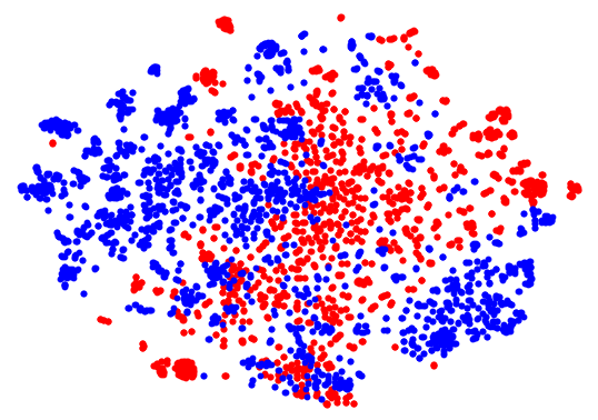
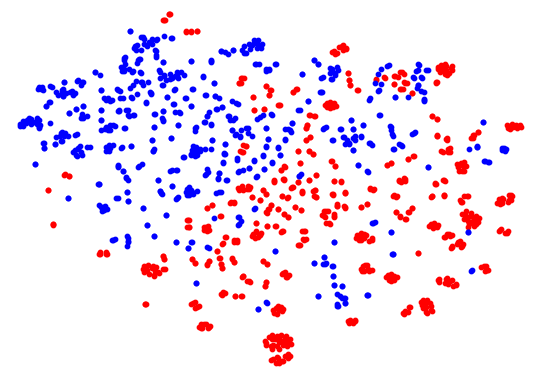
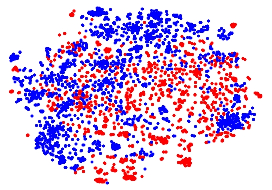
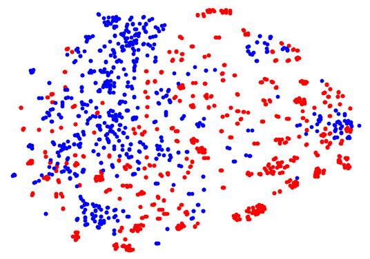
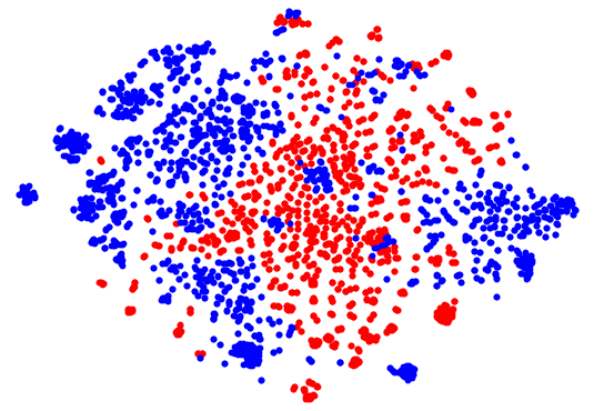
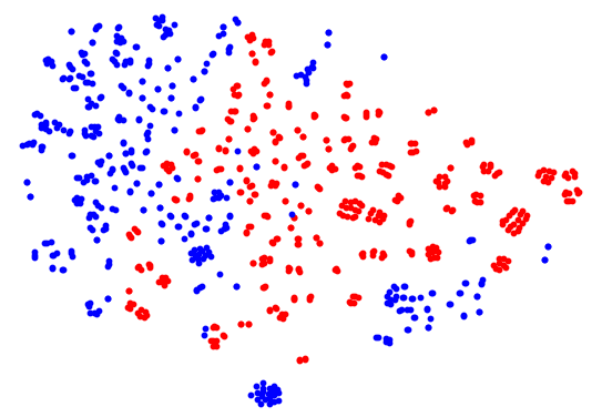
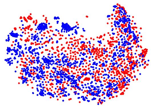
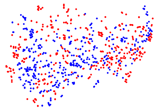
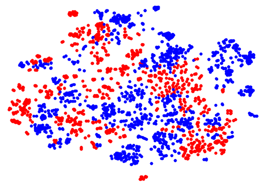
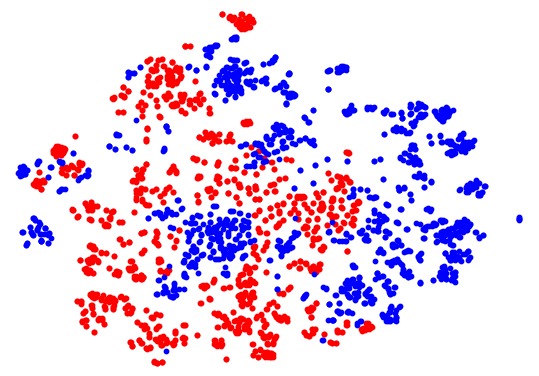
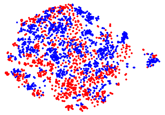
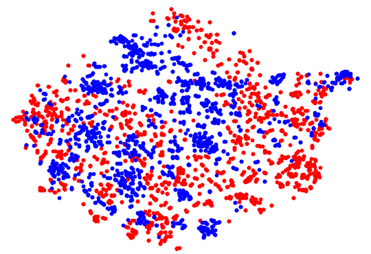
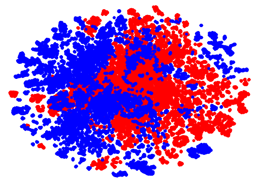
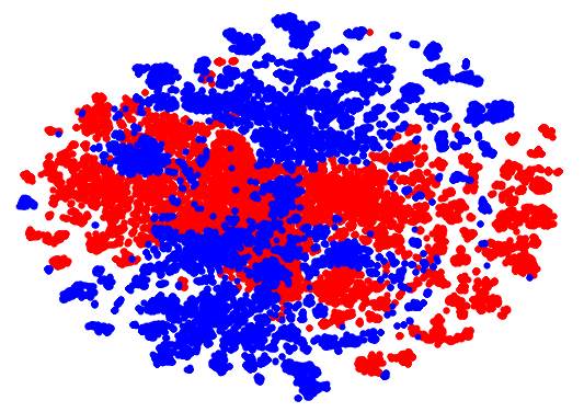
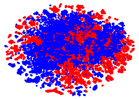
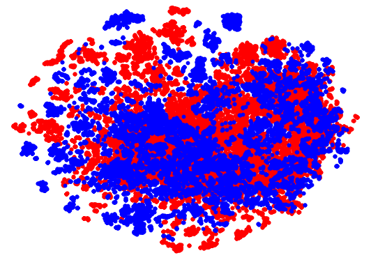
In this section, we extend the analysis of Sec. 4.3 to ablate over the effect that our alignment loss has on different resolution levels of the model. For this, in Figs. E, F and G we present the corresponding TSNE plots of the three majority action classes on 3 resolution levels. Here level 0 is the shallowest level and subsequent levels progressively reduce the resolution by 2. Observe that the influence of the alignment loss follows a similar pattern in all the resolutions. Concretely, in the three presented, we observe a considerable mixing between the source and target distributions (red and blue, respectively). This contrasts with the very clear disentanglement of the representations of both domains in the source-only version, where these present little to no overlap. We highlight what seems to be the only exception which is resolution level 3 of class 1. This one shows little improvement in the mixing of the distributions compared to the source-only variant.

We also find that our overall improvement of the mixing of the distributions is also consistent when analyzing the background class embeddings. Observe in Fig. H that in all 3 studied resolution levels, SADA improves very considerably the alignment, pushing the feature space of both domains to be domain invariant. This emphasizes the positive influence of the background alignment term of our loss (see Eq. 8 of the main paper).

E Study of the class embedding

B $\rightarrow$ {all \B} (EK100-EK55)
Strategy	mAP {10,20,30,40,50}%					Avg
One-hot	32.29	31.09	28.58	24.88	19.56	27.28
Random emb	30.71	29.50	27.43	23.78	18.52	25.99
Sinusoidal [55]	29.93	28.57	26.44	22.87	17.01	24.96
Learnable	32.69	31.49	29.17	25.51	19.72	27.72
B $\rightarrow$ {all\B} (EK55)
Strategy	mAP {10,20,30,40,50}%					Avg
One-hot	31.31	29.97	27.84	24.28	18.81	26.44
Random emb	31.38	30.01	27.94	24.13	18.70	26.43
Sinusoidal [55]	31.10	29.78	27.71	23.99	18.56	26.23
Learnable	31.68	30.32	28.37	24.55	19.09	26.80

Table A: Ablation of the effect of the use of a learnable class embedding over other static strategies.

One of the main contributions of our work is to adversarially align distributions in a class-wise fashion. Intuitively, this requires that our level-wise domain discriminator knows the class distribution that it is aligning. In this regard, in Sec. 3 we propose to concatenate to every anchor a learnable embeddings $e_{i}\in\mathbb{R}^{F}$ of its corresponding class $i$ (see Eq. 7 of the main paper). In this ablation, we empirically justify our choice. For this, we compare our approach with several possible alternative methods to encode a given class $i$. Concretely, we compare it with a naive one-hot encoding, a random class-wise dense encoding, and with the popular sinusoidal encoding [55].

In Tab. A we show the experimental results of each of these variants when tested in Scenarios 1 and 3 –presented in the main paper. In this regard, our results indicate that a naive one-hot encoding of a class is the best-performing non-learnable strategy, obtaining considerable improvements over the other two tested non-learnable baselines. This improvement is especially prominent in the first scenario, boosting the performance of the second-best-performing strategy by up to a relative $5\%$. Moreover, to our surprise, the popular Sinusoidal encoding [55] proves to be the worst-performing method, being consistently outperformed by even the random dense encoding. Finally, we highlight that in both scenarios the use of a learnable class embedding yields the best results, obtaining up to a $1.7\%$ relative improvement over the one-hot encoding strategy, which justifies our choice.

F Main ablations on other scenarios

In this section, we extend the ablation studies presented in Sec. 4.3 by analyzing two additional scenarios. Concretely, we compare the performance of SADA with the adaptations of different UDA methods, and with different variations of our loss, in Scenario 2 and 4.

F.1 Domain adaptation methods

In Tab. B we present the comparison of our proposed method to the other considered UDA baselines. This indicates that the first scenario (top), namely white new videos, poses important challenges when aligning its corresponding source and target domain. More specifically, in this scenario, all the considered UDA baselines worsen the performance of the source-only variant. The behavior of the baselines in the second scenario (down), namely white old, is similar. In this case, however, DANN [17] does improve the source-only variant. This is consistent with our observations from Sec. 4.2 where DANN [17] was also the best-performing baseline. Similarly, SSTDA [8] is the worst performing method in both scenarios, especially degrading in the second scenario (bottom) by up to a relative $-23.6\%$. In contrast, our method improves all the baselines in both scenarios, attaining up to a $6.46\%$ of relative improvement in the second scenario.

W $\rightarrow$ {all \W} (EK100-EK55)
Model	mAP {10,30,50}%			Avg
Source-only	34.41	30.58	21.00	28.66
DANN [18]	34.11	30.48	20.75	28.44
Semantic centroids [58]	32.95	29.22	19.20	27.12
SSTDA [8]	33.17	29.38	18.92	27.15
Ours (SADA)	34.86	31.16	21.46	29.16
W $\rightarrow$ {all \W} (EK55)
Model	mAP {10,30,50}%			Avg
Source-only	29.65	26.86	19.14	25.21
DANN [18]	31.32	28.55	20.10	26.65
Semantic centroids [58]	30.17	27.32	18.55	25.34
SSTDA [8]	23.45	20.95	13.37	19.26
Ours (SADA)	31.54	28.77	20.22	26.84

Table B: Ablation study on Scenarios 2 and 4, comparing the performance of our proposal SADA with the chosen domain adaptation methods coupled in our proposed architecture.

F.2 Ablation over variants of the SADA loss

W $\rightarrow$ {all \W} (EK100-EK55)
Local	Global	Bkg	mAP {10,30,50}%			Avg
			34.41	30.58	21.00	28.66
	$\textpdfrender{TextRenderingMode=FillStroke,LineWidth=1.0pt,}{\checkmark}$		34.11	30.48	20.75	28.44
		$\textpdfrender{TextRenderingMode=FillStroke,LineWidth=1.0pt,}{\checkmark}$	34.46	30.85	20.90	28.73
	$\textpdfrender{TextRenderingMode=FillStroke,LineWidth=1.0pt,}{\checkmark}$	$\textpdfrender{TextRenderingMode=FillStroke,LineWidth=1.0pt,}{\checkmark}$	34.63	31.08	21.26	28.99
$\textpdfrender{TextRenderingMode=FillStroke,LineWidth=1.0pt,}{\checkmark}$			33.47	29.91	20.17	27.85
$\textpdfrender{TextRenderingMode=FillStroke,LineWidth=1.0pt,}{\checkmark}$	$\textpdfrender{TextRenderingMode=FillStroke,LineWidth=1.0pt,}{\checkmark}$		32.84	29.06	19.41	27.10
$\textpdfrender{TextRenderingMode=FillStroke,LineWidth=1.0pt,}{\checkmark}$		$\textpdfrender{TextRenderingMode=FillStroke,LineWidth=1.0pt,}{\checkmark}$	34.86	31.16	21.46	29.16
W $\rightarrow$ {all \W} (EK55)
Local	Global	Bkg	mAP {10,30,50}%			Avg
			29.65	26.86	19.14	25.21
	$\textpdfrender{TextRenderingMode=FillStroke,LineWidth=1.0pt,}{\checkmark}$		31.32	28.55	20.10	26.65
		$\textpdfrender{TextRenderingMode=FillStroke,LineWidth=1.0pt,}{\checkmark}$	29.94	27.39	19.40	25.57
	$\textpdfrender{TextRenderingMode=FillStroke,LineWidth=1.0pt,}{\checkmark}$	$\textpdfrender{TextRenderingMode=FillStroke,LineWidth=1.0pt,}{\checkmark}$	30.86	28.02	19.84	26.57
$\textpdfrender{TextRenderingMode=FillStroke,LineWidth=1.0pt,}{\checkmark}$			30.84	27.98	19.37	26.06
$\textpdfrender{TextRenderingMode=FillStroke,LineWidth=1.0pt,}{\checkmark}$	$\textpdfrender{TextRenderingMode=FillStroke,LineWidth=1.0pt,}{\checkmark}$		29.77	27.10	18.70	25.19
$\textpdfrender{TextRenderingMode=FillStroke,LineWidth=1.0pt,}{\checkmark}$		$\textpdfrender{TextRenderingMode=FillStroke,LineWidth=1.0pt,}{\checkmark}$	31.54	28.77	20.22	26.84

Table C: Ablation study of the effect of several variations of our proposed SADA loss on Scenarios 2 and 4.

Similarly to Sec. 4.3, in Tab. C we ablate over different variants of our loss on Scenario 2 and 4. These scenarios define the source domain as white old and new counter kitchens and the rest as the target, respectively. Observe in this table that our main insights from Sec. 4.3 are mostly confirmed. Concretely, one of our main observations was that aligning the complete global distribution was generally preferable over aligning the partial background distribution only. This observation is satisfied in most of the scenarios that we study –with the exception of Scenario 3. Similarly, in Sec. 4.3 we argued that combining alignment loss that presented overlaps yielded also a decrease in performance. More in detail, this happens when we couple either the local or the background loss with a global alignment approach. In these cases, the embeddings have a double (simultaneous) alignment objective, which we argue is not desirable. As observed in Tab. C, this observation is also mostly satisfied in these scenarios as the combination of these losses yields a performance degradation in 7 of the 8 cases studied in this paper – included in Tab. C and Tab. 4 of the main paper.

G Ablation per class

	take	put	wash	open	close	insert	turn-on	cut	turn-off	pour
Src-only	24.20	29.30	37.30	32.69	23.89	10.98	37.39	18.18	26.24	18.55
DANN [18]	24.85	30.51	37.09	35.08	22.93	11.68	35.80	17.23	24.19	20.35
SADA (ours)	26.31	30.70	39.14	34.68	23.42	10.58	39.86	17.05	26.58	18.78

Table D: Per class mAPs (in percentage) obtained by the source only variation of our model, DANN [37] and our proposal SADA. These results correspond to Scenario 1, which defines black old kitchens as the source and the rest as a target.

	take	put	wash	open	close	insert	turn-on	cut	turn-off	pour
Src-only	24.11	25.69	29.77	31.96	27.8	6.69	25.52	34.16	17.48	29.18
DANN [18]	24.78	24.38	28.75	32.73	29.32	5.38	27.52	36.73	17.70	29.05
SADA (ours)	28.32	31.25	31.18	34.52	31.82	7.29	26.66	39.12	18.68	28.34

Table E: Per class mAPs (in percentage) obtained by the source only variation of our model, DANN [37] and our proposal SADA. These results correspond to Scenario 3, which defines black new kitchens as the source and the rest as a target.

In this section, we complement the analysis from Sec. 4.2 with the detailed class-wise metrics. Concretely, in Tab. D and Tab. E we show the respective class-wise mAP scores of the 10 considered classes on both Scenario 1 and 3. For the analysis, we also include the results obtained with the source-only variant of our model as well as our chosen DANN[17] baseline.

Observe that in Scenario 3 (see Tab. D) our model attains the best class-wise performance in 5 of the classes, while DANN [17] does so on 3, and the source-only model on 2. In contrast, in Scenario 1 (see Tab. E) our method obtains a much clearer improvement over the chosen baselines, yielding the best results in 8 of the 10 classes. Overall, we can observe that our method performs very well in the 3 majority classes of both scenarios, where we highlight the relative improvement of our model over DANN [17] of $28.17\%$ for the class put in Scenario 3. Moreover, our method fails to improve the performance of action pour in both scenarios, which we attribute to the lack of sufficient data to operate on our proposed methodology. We also highlight that as observed in Sec.4.2, Scenario 1 presents a more challenging setup, degrading the performance in other actions such as open, close, insert or cut. This indicates the existence of intrinsic qualitative aspects that harden the adaptation when dealing with old videos. This is not the case in Scenario 3, as aside from the aforementioned pour segments, it only fails to achieve the best results for the turn-on action.

H Ablation of the effect of negative anchors

B $\rightarrow$ {all \B} (EK100-EK55)
Filtered %	mAP {10,20,30,40,50}%					Avg
0%	32.69	31.49	29.17	25.51	19.72	27.72
25%	32.54	31.87	30.06	26.99	21.91	28.67
50%	34.46	33.55	31.29	27.59	21.18	29.61
75%	35.09	34.53	32.97	30.05	23.97	31.32
100%	35.57	35.24	34.16	30.72	24.50	32.04
B $\rightarrow$ {all\B} (EK55)
Filtered %	mAP {10,20,30,40,50}%					Avg
0%	31.60	30.29	28.22	24.47	18.98	26.71
25%	32.76	31.60	29.81	26.14	20.24	28.11
50%	35.25	34.25	32.68	29.25	23.01	30.89
75%	38.39	37.77	36.40	33.19	26.33	34.42
100%	43.93	43.59	42.61	39.26	31.85	40.25

Table F: Ablation of the effect of masking out different percentages of negative anchors during inference only.

B $\rightarrow$ {all \B} (EK100-EK55)
Filtered %	mAP {10,20,30,40,50}%					Avg
0%	32.69	31.49	29.17	25.51	19.72	27.72
25%	31.48	30.34	27.97	24.07	18.93	26.56
50%	32.11	31.11	29.25	25.85	20.72	27.81
75%	35.99	35.28	33.48	29.90	23.64	31.66
100%	37.53	37.06	35.73	32.34	26.45	33.82
B $\rightarrow$ {all\B} (EK55)
Filtered %	mAP {10,20,30,40,50}%					Avg
0%	31.60	30.29	28.22	24.47	18.98	26.71
25%	32.25	30.46	28.04	24.54	19.03	26.86
50%	33.43	32.06	29.98	26.44	20.55	28.49
75%	38.26	37.33	35.72	32.53	25.61	33.89
100%	47.08	46.69	45.65	42.31	34.42	43.23

Table G: Ablation of the effect of masking out different percentages of negative anchors during training and inference.

We argue that one of the main challenges that our method faces is how to deal with the excess of anchors predicted as class 0, which as described in Sec. 3.4 we refer to as negative anchors. These are the anchors that are not directly matched with a GT segment. In these cases, hence, we hope for the model to learn to identify these anchor embeddings as background, not predicting any action class during inference. This, however, is a cumbersome issue that most of the anchor-based methods face, which is exacerbated when doing domain adaptation in this complicated setup. In this case, it is not clear the amount of noise that these embeddings induce in the alignment strategy. Even though we leave a more thorough analysis of this issue as future work, in this section we aim to provide minimal proof of the potential negative effect that this has on the model’s performance.

Concretely, we propose an experiment where we progressively mask out the set of negative anchors. For this, in Tab. F we randomly mask out these only during inference. In other words, we leave all the training routines unchanged – thus considering all the anchors – but ensure that a percentage of the negative anchors are not considered during inference. This measures the predicting potential of a model that is able to perfectly deal with these embeddings. As observed in Tab. F, in both considered scenarios we observe a linear performance increase, reaching up to a $50.69\%$ relative improvement of the version with $100\%$ filtered negative anchors over the $0\%$ version. This is, the variant where only the positive anchors are considered over that containing both positive and all the negative ones.

In Tab. G we propose an alternative analysis. In this case, we do not only mask the negative anchors during inference but also during training. In this case, for instance, masking out $50\%$ of the negative anchors additionally implies not training any of the task losses on them, nor using them on our alignment loss. As observed in the results, masking them out entirely – i.e., $100\%$ – has an even bigger impact, reaching a relative improvement of $61.84\%$ over the $0\%$ version. Nevertheless, in this case, we observe that the improvement is no longer linear, and even worsens the performance for small percentages of masking. We hypothesize this is induced by a reduction of the training data of background class. In other words, while masking some negative embeddings has a positive effect, we must also consider the negative effect that having less training data has on the ones that we do consider. Hence, until this trade-off is dominated by the positive effect of masking out the majority of negative anchors, the improvement remains little to non-existent. In conclusion, these experiments emphasize the need for devising carefully designed models that can properly cope with this intrinsic limitations of anchor-based methods.

References

- Agarwal et al. [2020] Nakul Agarwal, Yi-Ting Chen, Behzad Dariush, and Ming-Hsuan Yang. Unsupervised domain adaptation for spatio-temporal action localization. arXiv preprint arXiv:2010.09211, 2020.
- Bodla et al. [2017] Navaneeth Bodla, Bharat Singh, Rama Chellappa, and Larry S Davis. Soft-nms–improving object detection with one line of code. In Proceedings of the IEEE international conference on computer vision, pages 5561–5569, 2017.
- Buch et al. [2017] Shyamal Buch, Victor Escorcia, Chuanqi Shen, Bernard Ghanem, and Juan Carlos Niebles. Sst: Single-stream temporal action proposals. In Proceedings of the IEEE conference on Computer Vision and Pattern Recognition, pages 2911–2920, 2017.
- Carion et al. [2020] Nicolas Carion, Francisco Massa, Gabriel Synnaeve, Nicolas Usunier, Alexander Kirillov, and Sergey Zagoruyko. End-to-end object detection with transformers. In Computer Vision–ECCV 2020: 16th European Conference, Glasgow, UK, August 23–28, 2020, Proceedings, Part I 16, pages 213–229. Springer, 2020.
- Carreira and Zisserman [2017] Joao Carreira and Andrew Zisserman. Quo vadis, action recognition? a new model and the kinetics dataset. In proceedings of the IEEE Conference on Computer Vision and Pattern Recognition, pages 6299–6308, 2017.
- Chao et al. [2018] Yu-Wei Chao, Sudheendra Vijayanarasimhan, Bryan Seybold, David A Ross, Jia Deng, and Rahul Sukthankar. Rethinking the faster r-cnn architecture for temporal action localization. In Proceedings of the IEEE conference on computer vision and pattern recognition, pages 1130–1139, 2018.
- Chen et al. [2019] Min-Hung Chen, Zsolt Kira, Ghassan AlRegib, Jaekwon Yoo, Ruxin Chen, and Jian Zheng. Temporal attentive alignment for large-scale video domain adaptation. In Proceedings of the IEEE/CVF International Conference on Computer Vision, pages 6321–6330, 2019.
- Chen et al. [2020] Min-Hung Chen, Baopu Li, Yingze Bao, Ghassan AlRegib, and Zsolt Kira. Action segmentation with joint self-supervised temporal domain adaptation. In Proceedings of the IEEE/CVF Conference on Computer Vision and Pattern Recognition, pages 9454–9463, 2020.
- Chen et al. [2018] Yuhua Chen, Wen Li, Christos Sakaridis, Dengxin Dai, and Luc Van Gool. Domain adaptive faster r-cnn for object detection in the wild. In Proceedings of the IEEE conference on computer vision and pattern recognition, pages 3339–3348, 2018.
- Csurka [2017a] Gabriela Csurka. A comprehensive survey on domain adaptation for visual applications. Domain adaptation in computer vision applications, pages 1–35, 2017a.
- Csurka [2017b] Gabriela Csurka. Domain adaptation for visual applications: A comprehensive survey. arXiv preprint arXiv:1702.05374, 2017b.
- Cui et al. [2020] Shuhao Cui, Shuhui Wang, Junbao Zhuo, Chi Su, Qingming Huang, and Qi Tian. Gradually vanishing bridge for adversarial domain adaptation. In Proceedings of the IEEE/CVF conference on computer vision and pattern recognition, pages 12455–12464, 2020.
- Damen et al. [2018] Dima Damen, Hazel Doughty, Giovanni Maria Farinella, Sanja Fidler, Antonino Furnari, Evangelos Kazakos, Davide Moltisanti, Jonathan Munro, Toby Perrett, Will Price, and Michael Wray. Scaling egocentric vision: The epic-kitchens dataset. In European Conference on Computer Vision (ECCV), 2018.
- Damen et al. [2022] Dima Damen, Hazel Doughty, Giovanni Maria Farinella, Antonino Furnari, Jian Ma, Evangelos Kazakos, Davide Moltisanti, Jonathan Munro, Toby Perrett, Will Price, and Michael Wray. Rescaling egocentric vision: Collection, pipeline and challenges for epic-kitchens-100. International Journal of Computer Vision (IJCV), 130:33–55, 2022.
- Fathi et al. [2011] Alireza Fathi, Xiaofeng Ren, and James M Rehg. Learning to recognize objects in egocentric activities. In CVPR 2011, pages 3281–3288. IEEE, 2011.
- Feichtenhofer et al. [2019] Christoph Feichtenhofer, Haoqi Fan, Jitendra Malik, and Kaiming He. Slowfast networks for video recognition. In Proceedings of the IEEE/CVF international conference on computer vision, pages 6202–6211, 2019.
- Ganin and Lempitsky [2015] Yaroslav Ganin and Victor Lempitsky. Unsupervised domain adaptation by backpropagation. In International conference on machine learning, pages 1180–1189. PMLR, 2015.
- Ganin et al. [2016] Yaroslav Ganin, Evgeniya Ustinova, Hana Ajakan, Pascal Germain, Hugo Larochelle, François Laviolette, Mario Marchand, and Victor Lempitsky. Domain-adversarial training of neural networks. The journal of machine learning research, 17(1):2096–2030, 2016.
- Grandvalet and Bengio [2004] Yves Grandvalet and Yoshua Bengio. Semi-supervised learning by entropy minimization. Advances in neural information processing systems, 17, 2004.
- Haeusser et al. [2017] Philip Haeusser, Thomas Frerix, Alexander Mordvintsev, and Daniel Cremers. Associative domain adaptation. In Proceedings of the IEEE international conference on computer vision, pages 2765–2773, 2017.
- HassanPour Zonoozi and Seydi [2023] Mahta HassanPour Zonoozi and Vahid Seydi. A survey on adversarial domain adaptation. Neural Processing Letters, 55(3):2429–2469, 2023.
- Hoffman et al. [2017] Judy Hoffman, Eric Tzeng, Trevor Darrell, and Kate Saenko. Simultaneous deep transfer across domains and tasks. Domain Adaptation in Computer Vision Applications, pages 173–187, 2017.
- Hu et al. [2023] Sijie Hu, Fabien Bonardi, Samia Bouchafa, and Désiré Sidibé. Multi-modal unsupervised domain adaptation for semantic image segmentation. Pattern Recognition, 137:109299, 2023.
- Idrees et al. [2017] Haroon Idrees, Amir R Zamir, Yu-Gang Jiang, Alex Gorban, Ivan Laptev, Rahul Sukthankar, and Mubarak Shah. The thumos challenge on action recognition for videos “in the wild”. Computer Vision and Image Understanding, 155:1–23, 2017.
- Jamal et al. [2018] Arshad Jamal, Vinay P Namboodiri, Dipti Deodhare, and KS Venkatesh. Deep domain adaptation in action space. In BMVC, page 5, 2018.
- Kang et al. [2019] Guoliang Kang, Lu Jiang, Yi Yang, and Alexander G Hauptmann. Contrastive adaptation network for unsupervised domain adaptation. In Proceedings of the IEEE/CVF conference on computer vision and pattern recognition, pages 4893–4902, 2019.
- Kay et al. [2017] Will Kay, Joao Carreira, Karen Simonyan, Brian Zhang, Chloe Hillier, Sudheendra Vijayanarasimhan, Fabio Viola, Tim Green, Trevor Back, Paul Natsev, et al. The kinetics human action video dataset. arXiv preprint arXiv:1705.06950, 2017.
- Koniusz et al. [2017] Piotr Koniusz, Yusuf Tas, and Fatih Porikli. Domain adaptation by mixture of alignments of second-or higher-order scatter tensors. In Proceedings of the IEEE conference on computer vision and pattern recognition, pages 4478–4487, 2017.
- Kuehne et al. [2014] H. Kuehne, A. B. Arslan, and T. Serre. The language of actions: Recovering the syntax and semantics of goal-directed human activities. In Proceedings of Computer Vision and Pattern Recognition Conference (CVPR), 2014.
- Li et al. [2023] Yundong Li, Longxia Guo, and Yizheng Ge. Pseudo labels for unsupervised domain adaptation: A review. Electronics, 12(15):3325, 2023.
- Li and Yao [2021] Zhihui Li and Lina Yao. Three birds with one stone: Multi-task temporal action detection via recycling temporal annotations. In Proceedings of the IEEE/CVF Conference on Computer Vision and Pattern Recognition, pages 4751–4760, 2021.
- Lin et al. [2021] Chuming Lin, Chengming Xu, Donghao Luo, Yabiao Wang, Ying Tai, Chengjie Wang, Jilin Li, Feiyue Huang, and Yanwei Fu. Learning salient boundary feature for anchor-free temporal action localization. In Proceedings of the IEEE/CVF Conference on Computer Vision and Pattern Recognition, pages 3320–3329, 2021.
- Lin et al. [2017a] Tianwei Lin, Xu Zhao, and Zheng Shou. Single shot temporal action detection. In Proceedings of the 25th ACM international conference on Multimedia, pages 988–996, 2017a.
- Lin et al. [2017b] Tsung-Yi Lin, Priya Goyal, Ross Girshick, Kaiming He, and Piotr Dollár. Focal loss for dense object detection. In Proceedings of the IEEE international conference on computer vision, pages 2980–2988, 2017b.
- Liu et al. [2021] Xiaolong Liu, Qimeng Wang, Yao Hu, Xu Tang, Song Bai, and Xiang Bai. End-to-end temporal action detection with transformer. arXiv preprint arXiv:2106.10271, 2021.
- Liu et al. [2022] Xiaolong Liu, Song Bai, and Xiang Bai. An empirical study of end-to-end temporal action detection. In Proceedings of the IEEE/CVF Conference on Computer Vision and Pattern Recognition, pages 20010–20019, 2022.
- Long et al. [2015] Mingsheng Long, Yue Cao, Jianmin Wang, and Michael Jordan. Learning transferable features with deep adaptation networks. In International conference on machine learning, pages 97–105. PMLR, 2015.
- Long et al. [2017] Mingsheng Long, Zhangjie Cao, Jianmin Wang, and Michael I Jordan. Domain adaptation with randomized multilinear adversarial networks. arXiv preprint arXiv:1705.10667, 2017.
- Loshchilov and Hutter [2017] Ilya Loshchilov and Frank Hutter. Decoupled weight decay regularization. arXiv preprint arXiv:1711.05101, 2017.
- Lu et al. [2023] Yifan Lu, Gurkirt Singh, Suman Saha, and Luc Van Gool. Exploiting instance-based mixed sampling via auxiliary source domain supervision for domain-adaptive action detection. In Proceedings of the IEEE/CVF Winter Conference on Applications of Computer Vision, pages 4145–4156, 2023.
- Motiian et al. [2017] Saeid Motiian, Marco Piccirilli, Donald A Adjeroh, and Gianfranco Doretto. Unified deep supervised domain adaptation and generalization. In Proceedings of the IEEE international conference on computer vision, pages 5715–5725, 2017.
- Oza et al. [2023] Poojan Oza, Vishwanath A Sindagi, Vibashan Vishnukumar Sharmini, and Vishal M Patel. Unsupervised domain adaptation of object detectors: A survey. IEEE Transactions on Pattern Analysis and Machine Intelligence, 2023.
- Pan et al. [2020] Boxiao Pan, Zhangjie Cao, Ehsan Adeli, and Juan Carlos Niebles. Adversarial cross-domain action recognition with co-attention. In Proceedings of the AAAI Conference on Artificial Intelligence, pages 11815–11822, 2020.
- Pan and Yang [2009] Sinno Jialin Pan and Qiang Yang. A survey on transfer learning. IEEE Transactions on knowledge and data engineering, 22(10):1345–1359, 2009.
- Paszke et al. [2019] Adam Paszke, Sam Gross, Francisco Massa, Adam Lerer, James Bradbury, Gregory Chanan, Trevor Killeen, Zeming Lin, Natalia Gimelshein, Luca Antiga, et al. Pytorch: An imperative style, high-performance deep learning library. Advances in neural information processing systems, 32, 2019.
- Qing et al. [2021] Zhiwu Qing, Haisheng Su, Weihao Gan, Dongliang Wang, Wei Wu, Xiang Wang, Yu Qiao, Junjie Yan, Changxin Gao, and Nong Sang. Temporal context aggregation network for temporal action proposal refinement. In Proceedings of the IEEE/CVF conference on computer vision and pattern recognition, pages 485–494, 2021.
- Sankaranarayanan et al. [2018] Swami Sankaranarayanan, Yogesh Balaji, Arpit Jain, Ser Nam Lim, and Rama Chellappa. Learning from synthetic data: Addressing domain shift for semantic segmentation. In Proceedings of the IEEE conference on computer vision and pattern recognition, pages 3752–3761, 2018.
- Sener et al. [2016] Ozan Sener, Hyun Oh Song, Ashutosh Saxena, and Silvio Savarese. Learning transferrable representations for unsupervised domain adaptation. Advances in neural information processing systems, 29, 2016.
- Shi et al. [2023] Dingfeng Shi, Yujie Zhong, Qiong Cao, Lin Ma, Jia Li, and Dacheng Tao. Tridet: Temporal action detection with relative boundary modeling. In Proceedings of the IEEE/CVF Conference on Computer Vision and Pattern Recognition, pages 18857–18866, 2023.
- Shou et al. [2017] Zheng Shou, Jonathan Chan, Alireza Zareian, Kazuyuki Miyazawa, and Shih-Fu Chang. Cdc: Convolutional-de-convolutional networks for precise temporal action localization in untrimmed videos. In Proceedings of the IEEE conference on computer vision and pattern recognition, pages 5734–5743, 2017.
- Sridhar et al. [2021] Deepak Sridhar, Niamul Quader, Srikanth Muralidharan, Yaoxin Li, Peng Dai, and Juwei Lu. Class semantics-based attention for action detection. In Proceedings of the IEEE/CVF International Conference on Computer Vision, pages 13739–13748, 2021.
- Tan et al. [2021] Jing Tan, Jiaqi Tang, Limin Wang, and Gangshan Wu. Relaxed transformer decoders for direct action proposal generation. In Proceedings of the IEEE/CVF international conference on computer vision, pages 13526–13535, 2021.
- Tian et al. [2019] Zhi Tian, Chunhua Shen, Hao Chen, and Tong He. Fcos: Fully convolutional one-stage object detection. In Proceedings of the IEEE/CVF international conference on computer vision, pages 9627–9636, 2019.
- Tzeng et al. [2017] Eric Tzeng, Judy Hoffman, Kate Saenko, and Trevor Darrell. Adversarial discriminative domain adaptation. In Proceedings of the IEEE conference on computer vision and pattern recognition, pages 7167–7176, 2017.
- Vaswani et al. [2017] Ashish Vaswani, Noam Shazeer, Niki Parmar, Jakob Uszkoreit, Llion Jones, Aidan N Gomez, Łukasz Kaiser, and Illia Polosukhin. Attention is all you need. Advances in neural information processing systems, 30, 2017.
- Wang et al. [2019] Ximei Wang, Ying Jin, Mingsheng Long, Jianmin Wang, and Michael I Jordan. Transferable normalization: Towards improving transferability of deep neural networks. Advances in neural information processing systems, 32, 2019.
- Wei et al. [2023] Pengfei Wei, Lingdong Kong, Xinghua Qu, Yi Ren, Jing Jiang, Xiang Yin, et al. Unsupervised video domain adaptation for action recognition: A disentanglement perspective. In Thirty-seventh Conference on Neural Information Processing Systems, 2023.
- Xie et al. [2018] Shaoan Xie, Zibin Zheng, Liang Chen, and Chuan Chen. Learning semantic representations for unsupervised domain adaptation. In International conference on machine learning, pages 5423–5432. PMLR, 2018.
- Xu et al. [2021] Yuecong Xu, Jianfei Yang, Haozhi Cao, Zhenghua Chen, Qi Li, and Kezhi Mao. Partial video domain adaptation with partial adversarial temporal attentive network. In Proceedings of the IEEE/CVF International Conference on Computer Vision, pages 9332–9341, 2021.
- Xu et al. [2022] Yuecong Xu, Haozhi Cao, Kezhi Mao, Zhenghua Chen, Lihua Xie, and Jianfei Yang. Aligning correlation information for domain adaptation in action recognition. IEEE Transactions on Neural Networks and Learning Systems, 2022.
- Yuan et al. [2017] Zehuan Yuan, Jonathan C Stroud, Tong Lu, and Jia Deng. Temporal action localization by structured maximal sums. In Proceedings of the IEEE Conference on Computer Vision and Pattern Recognition, pages 3684–3692, 2017.
- Zhang et al. [2022] Chen-Lin Zhang, Jianxin Wu, and Yin Li. Actionformer: Localizing moments of actions with transformers. In European Conference on Computer Vision, pages 492–510. Springer, 2022.
- Zhang et al. [2020] Shifeng Zhang, Cheng Chi, Yongqiang Yao, Zhen Lei, and Stan Z Li. Bridging the gap between anchor-based and anchor-free detection via adaptive training sample selection. In Proceedings of the IEEE/CVF conference on computer vision and pattern recognition, pages 9759–9768, 2020.
- Zhao et al. [2019] Hang Zhao, Antonio Torralba, Lorenzo Torresani, and Zhicheng Yan. Hacs: Human action clips and segments dataset for recognition and temporal localization. In Proceedings of the IEEE/CVF International Conference on Computer Vision, pages 8668–8678, 2019.
- Zhao et al. [2020] Peisen Zhao, Lingxi Xie, Chen Ju, Ya Zhang, Yanfeng Wang, and Qi Tian. Bottom-up temporal action localization with mutual regularization. In Computer Vision–ECCV 2020: 16th European Conference, Glasgow, UK, August 23–28, 2020, Proceedings, Part VIII 16, pages 539–555. Springer, 2020.
- Zhao et al. [2017] Yue Zhao, Yuanjun Xiong, Limin Wang, Zhirong Wu, Xiaoou Tang, and Dahua Lin. Temporal action detection with structured segment networks. In Proceedings of the IEEE international conference on computer vision, pages 2914–2923, 2017.